Electricity markets increasingly expose stochastic energy generators to arbitrage opportunities between the day-ahead and balancing markets, driven by widening price spreads. However, opportunistic bidding, deliberately deviating from the production forecast to exploit anticipated price spreads, carries significant risk, and existing frameworks rarely offer explainable, risk-aware decision support. We propose a predict-then-contextual-optimize framework that decomposes the day-ahead bidding decision into three explicit stages to decide, when to engage in arbitrage, in what direction, and to what extent. A probabilistic binary classifier with confidence thresholds determines whether the predicted price spread is sufficiently confident to justify an opportunistic bid. Otherwise, the trader defaults to an arbitrage-free bid equal to the power forecast. A linear decision policy learned for each class via contextual optimization determines the magnitude of the bid deviation from the power forecast. The framework accommodates both standalone renewable generation and hybrid power plants combining renewable generation with other assets, such as an electrolyzer. We evaluate the framework on a real wind farm in the European bidding zones DK1 and DE/LU using a rolling-window procedure and compare it against several benchmark bidding strategies. The results show that the proposed framework increases mean profit relative to an arbitrage-free benchmark, reaching an improvement of about 7% for the hybrid power plant in DK1. The largest gains occur when distributional drift between training and testing windows is low, while the co-located electrolyzer further increases arbitrage value by providing additional operational flexibility.

1 Introduction↩︎

A stochastic energy generator, e.g., a wind farm, typically sells a majority of its energy for a delivery period \(t\) in the day-ahead electricity market at price \(\lambda_t^{\rm DA}\) (€/MWh). One day prior to physical delivery \(t\), it needs to decide on the amount of energy \(p_t^{\rm DA}\) (MWh) to bid into the day-ahead market, given a production forecast \(\hat{P}_t^{\rm W}\) (MWh) and assuming a marginal production cost of €0/MWh. Given the realized production \(P_t^{\rm W}\) after the delivery period \(t\), any physical deviation from the contracted energy \(p_t^{\rm B} = P_t^{\rm W} - p_t^{\rm DA}\) is settled post-delivery in the balancing market at price \(\lambda_t^{\rm B}\) (€/MWh), which may be lower than, equal to, or higher than \(\lambda_t^{\rm DA}\), depending on the system need, i.e., whether there is a power deficit or surplus in the system. If the trader bids its production forecast \(\hat{P}_t^{\rm W}\), we refer to this as an arbitrage-free bid, since the trader does not intentionally exploit a forecasted price difference between the two markets. By contrast, if the trader deliberately bids above the forecast to benefit from a positive price spread \(\Delta\lambda_t = \lambda_t^{\rm DA} - \lambda_t^{\rm B}\), we call this an opportunistic long arbitrage bid. If the trader bids below the forecast to benefit from a negative price spread, we call this an opportunistic short arbitrage bid.

However, both market prices \((\lambda_t^{\rm DA}, \lambda_t^{\rm B})\) are uncertain at the time of decision making in the day-ahead stage, introducing substantial risk to opportunistic bidding strategies. Recent market developments further motivate this problem, as increasing renewable penetration, higher balancing-price volatility, and ongoing changes in balancing market design make arbitrage opportunities between the day-ahead and balancing markets more relevant. At the same time, these trends also make opportunistic arbitrage decisions riskier and more difficult. Therefore, an effective trading strategy needs to account for the uncertainty of \(\Delta\lambda_t\) and explicitly consider the risk of each decision. In addition, the trading framework should be pragmatic for power traders, i.e., computationally efficient and explainable. The problem becomes even more challenging for co-located assets with temporal constraints, such as a hybrid power plant (HPP) combining renewable generation and electrolyzer operation. In this work, we focus solely on the perspective of a price-taking power trader and leave the system-level implications of opportunistic arbitrage bidding, such as effects on market social welfare, for future work.

1.1 Literature Review↩︎

Literature on bidding stochastic renewable energy into the day-ahead market is mostly developed under dual-price balancing schemes, where separate imbalance prices apply depending on whether the power trader’s imbalance supports or aggravates the system need. In this setting, the trader faces different prices for upward and downward deviations, and any imbalance is typically penalized relative to the day-ahead position. The resulting bidding problem is therefore commonly formulated as a classical newsvendor-type problem [1], [2]. Under such a dual-price scheme, the trader is primarily exposed to risk of imbalance cost, while intentional arbitrage between the day-ahead and balancing markets is structurally limited. By contrast, several European markets have recently moved toward harmonized imbalance settlement rules, including single-price balancing, where a balance responsible party is settled at one balancing price irrespective of the direction of its imbalance [3], [4]. This imbalance settlement mechanism that exposes stochastic producers to price risk can also create opportunities for opportunistic arbitrage between the day-ahead and balancing markets. We describe this market design in more detail in Section 2. Despite this practical relevance, there is still limited literature on opportunistic arbitrage bidding for stochastic producers under single-price balancing.

A structurally related problem has been studied more extensively in U.S. two-settlement electricity markets under the terms virtual bidding or convergence bidding. Virtual bidding allows purely financial participants to take positions in the day-ahead market and close them in the real-time market without holding physical generation or consumption assets. In this setting, a trader can submit an increment or decrement bid in the day-ahead market and offset this position in real time, thereby arbitraging the price spread between the two settlements. Several studies analyze virtual bidding from a market design perspective, showing that it can improve liquidity, price convergence, and market efficiency under suitable conditions [5]–[7]. However, other works show that these benefits may not materialize when virtual bids interact with non-convex market clearing procedures, transmission constraints, or financial transmission rights, and that virtual bidding may also create incentives for market manipulation [8]–[10]. These studies are important for understanding the market-level implications of arbitrage, but they differ from our focus. In this paper, we take the perspective of a price-taking power trader and study how such a trader should make risk-aware arbitrage decisions. We do not analyze the welfare, liquidity, or price convergence impacts of opportunistic arbitrage bidding, which we leave for future work.

Within the literature taking a power traders perspective, several papers propose optimization or learning methods for virtual trading. [11] develops stochastic optimization models for increment and decrement bidding curves using generated price scenarios and conditional value-at-risk (CVaR) constraints for risk management. [12] studies algorithmic virtual bidding from an online learning perspective and proposes a dynamic programming method that sequentially allocates a fixed budget across multiple location-hour opportunities without assuming knowledge of the underlying price distribution. More recent learning based approaches also use historical data to predict or exploit day-ahead and real-time price spreads [13]. These papers demonstrate the value of data-driven and risk-aware methods for arbitrage bidding. However, they are primarily designed for financial traders in U.S. markets and do not consider the physical constraints of renewable generators or co-located assets. Moreover, the link between observable market conditions, price spread uncertainty, and the final arbitrage decision is often not explainable. Although the models may use historical spread data, they do not explicitly explain when arbitrage should be avoided, what drives the predicted arbitrage direction, or how a trader can tune its risk exposure in a practically explainable way.

The literature on European single-price balancing markets for stochastic assets is more limited. [14] studies risk-constrained trading strategies for stochastic generation under a single-price balancing market by adapting the all-or-nothing strategy, that will be discussed in Section 2.2, using system imbalance state predictions. However, predicting the system imbalance state may be insufficient when the relevant economic quantity is the price spread between the day-ahead and balancing markets. [15] introduces a risk certificate that bounds the balancing-market position and thereby restricts the all-or-nothing bid. This provides a useful way to limit exposure, but the balancing price, which is the main source of uncertainty in the arbitrage decision, is represented by a simplified rolling average. [16] learns linear decision policies for wind and hydrogen trading with risk constraints such as CVaR, following the prescriptive analytics paradigm of [17] and the broader contextual optimization literature reviewed in [18]. This approach directly maps contextual features to decisions and is computationally efficient, but the prediction of the price spread is embedded implicitly in the policy learning step rather than being made explicit to the trader.

Across these streams, two research gaps remain. First, existing arbitrage-bidding models [11]–[16] rarely provide an explainable decomposition of the decision into when to engage in arbitrage, which direction to take, and how large the position should be. In principle, the models in [8], [11], [19] could merge these layers and optimize a single arbitrage quantity directly, where zero means no arbitrage, a positive value means a long position, and a negative value means a short position. However, such an integrated formulation obscures the economic logic of the decision and may require solving an optimization problem even in situations where the price spread signal is too uncertain and arbitrage should be avoided. Second, existing approaches offer limited practical tools for managing the trader’s risk preference. Some models are risk-neutral [20], [21], while others impose risk-aversion through CVaR optimization [22] or scenario-based formulations [23], [24]. In many cases, however, it is unclear how a trader can tune the degree of opportunism in deployment and understand the resulting profit–risk trade-off.

1.2 Contributions↩︎

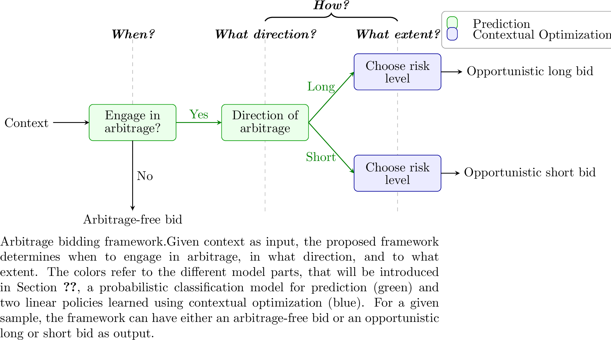As mentioned above, the existing bidding strategies mainly focus on how to trade in the market, often producing arbitrage bids implicitly as the output of an optimization or learning model. However, this makes it difficult for the trader to understand when arbitrage is justified and when it should be avoided. To overcome this issue, our framework combines the logic of predict-then-optimize with contextual optimization. In the first step, we predict the price spread \(\boldsymbol{\Delta\lambda}\) from contextual features. In the second step, conditional on this prediction, we use contextual optimization to learn bidding policies that map the same contextual features directly to day-ahead bid quantities. We therefore refer to the proposed methodology as a predict-then-contextual-optimize framework. This positioning connects our approach to the predict-then-optimize literature [25] and the contextual optimization literature [17], [18], while preserving the explainability needed for practical bidding decisions. The proposed framework explicitly decomposes the trading decision into three stages, as illustrated in Figure 1:

1. When to bid opportunistically. We introduce a probabilistic binary classifier coupled with direction-specific confidence thresholds on the predicted price spread \(\Delta\lambda_t\) to identify when opportunistic bidding is justified. When the prediction is too uncertain, the framework defaults to place an arbitrage-free bid, e.g.,day-ahead bid equal to the power forecast.

2. Direction of the opportunistic bid. Conditional on engaging in arbitrage, the framework determines whether the trader should take a long or short position relative to the production forecast. A predicted positive price spread \(\Delta\lambda_t\) motivates bidding above the forecast (opportunistic long bid), while a predicted negative price spread motivates bidding below the forecast (opportunistic short bid).

3. Extent of the position. The magnitude of the long or short position is determined based on a linear decision policy per each class that is trained by maximizing a weighted combination of expected profit and CVaR of the profit via contextual optimization. This provides a second layer of risk management in addition to the confidence thresholds.

This risk-aware structure of three stages preserves pragmaticality, enables fast decision-making at testing time, and allows operational constraints, such as those of a co-located electrolyzer in a HPP, to be incorporated directly into policy training without structural modification of the framework. In addition, we present a realistic case study demonstrating the framework on a real wind farm in the DK1 and DE/LU bidding zones, comparing models of varying complexity and quantifying the profit–risk trade-off introduced by the confidence thresholds.

The remainder of the paper is structured as follows: Section 2 provides market preliminaries and a detailed problem overview. Section 3 details the training phase, covering both the classification (Section 3.1) and the contextual optimization problem (Section 3.2). Section 4 presents the full testing phase, describing how a trained model processes contextual features to determine optimal day-ahead bids and compute realized profits, whereas Section 5 provides numerical results. Finally, Section 6 concludes the paper.

2 Preliminaries and Overview↩︎

This section establishes the foundations for the bidding framework developed in the paper. Section 2.1 introduces the market structure and motivates the problem by characterizing the statistical properties of the day-ahead (\(\boldsymbol{\lambda}^{\rm DA}\)) and balancing prices (\(\boldsymbol{\lambda}^{\rm B}\)) over the previous years. Building on this, Section 2.2 formalizes the problem setting, presents the overview of the three stage decision framework, and describes the rolling window procedure used throughout the paper to evaluate the out-of-sample performance.

2.1 Market Related Preliminaries↩︎

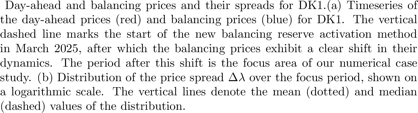As introduced in Section 1, we focus on a two stage bidding problem. In specific, the first trading floor is the day-ahead market, in which bids are placed on the day before, \(d-1\), for delivery periods on day \(d\). Hence, all bids of delivery periods of day \(d\) need to be submitted before gate closure on \(d-1\). In Europe, the day-ahead market has gate closure at 12pm on \(d-1\) and the delivery periods have recently transitioned from 60min market time unit (MTU) to 15min MTU quadrupling the number of product to 96 for delivery day \(d\). Therefore, the market clearing yields day-ahead prices \(\boldsymbol{\lambda}^{\rm DA}_d \in \mathbb{R}^{96}\) for each delivery day \(d\). The second trading floor is the balancing market, in which any imbalance from previous floors is automatically settled ex-post after realization. In Europe, the balancing market has also recently shifted the MTU from 60min to 15min yielding balancing prices \(\boldsymbol{\lambda}^{\rm B}_d \in \mathbb{R}^{96}\) for day \(d\). As the MTU is reduced, the power system can switch more frequently between surplus and deficit conditions within the delivery day. These more frequent changes in the system imbalance condition can increase balancing-price volatility and enlarge the price spread between the day-ahead and balancing markets. Consequently, arbitrage becomes more relevant, as traders have more opportunities to benefit from deviations between the two market prices.

In Figure 2a, the day-ahead prices (red) and balancing prices (blue) are shown for DK1 from January 2023 to February 2026. The balancing prices exhibit a clear shift in dynamics, caused by the new activation method for tertiary balancing reserves [26]. We focus on the period after this shift, as it is characterized by much higher price spreads and, therefore, greater arbitrage opportunities. The distribution of the price spreads \(\boldsymbol{\Delta\lambda}\) over the focus period is shown in Figure 2b on a logarithmic scale. While most samples have a positive spread (median price spread = €16.7/MWh), the negative spread has a much heavier tail pushing the distributions mean (€-3.3/MWh) well below its median. This tail is mainly driven by the high balancing price peaks that are also visible in Figure 2a.

2.2 Problem Overview↩︎

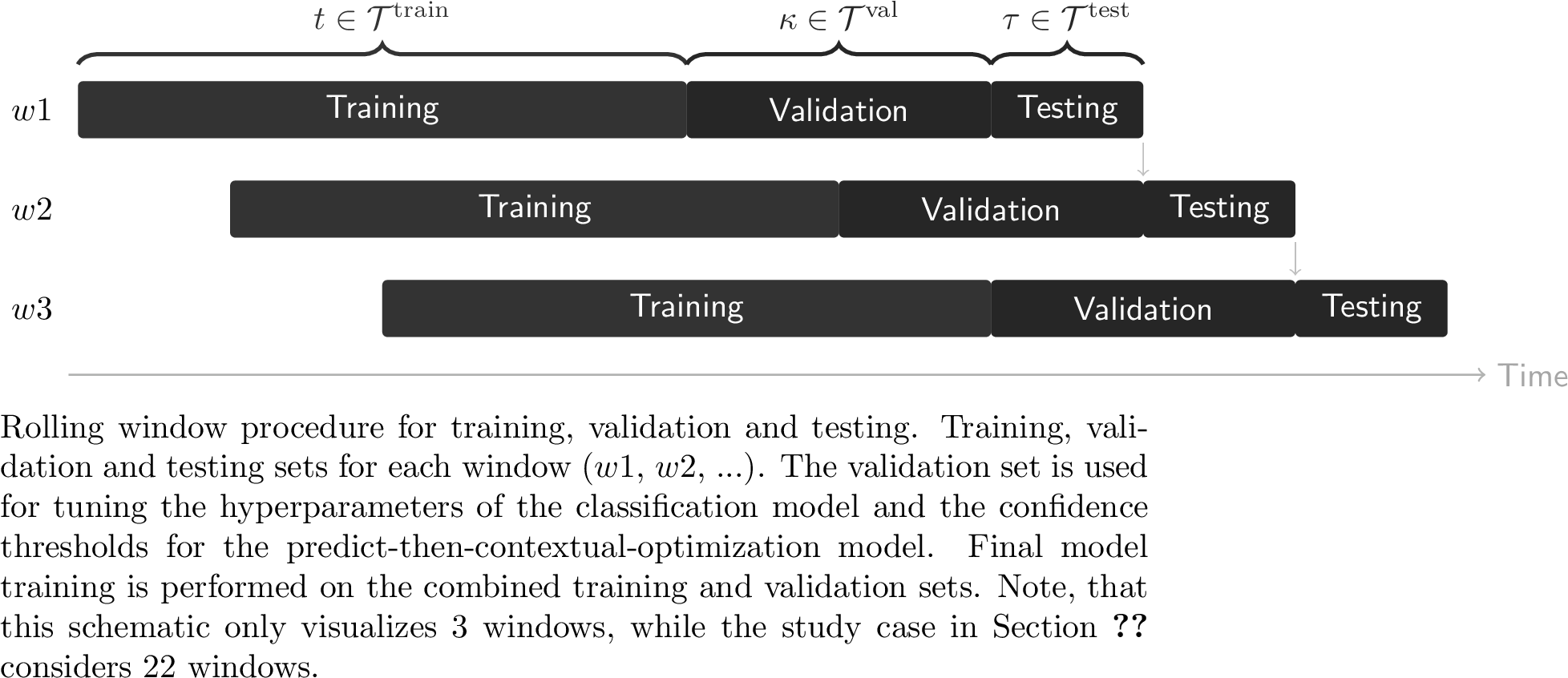We consider a price-taking power trader, either a standalone wind farm (wind-only) or a HPP consisting of a co-located wind farm and electrolyzer that participates in two sequential electricity markets, the day-ahead market and the balancing market. Recall, the power trader submits the day-ahead bid \(p_t^{\rm DA}\), before the wind production \(P_t^{\rm W}\), day-ahead and balancing prices, \(\lambda_t^{\rm DA}\) and \(\lambda_t^{\rm B}\), are realized. Under the current market regulation, the optimal bidding strategy follows a binary all-or-nothing rule. To see this, consider the profit maximization problem for a wind farm over a single delivery period \(t\): \[\tag{1} \begin{align} \underset{p_t^{\rm DA},p_t^{\rm B}}{\max} \quad & \lambda^{\rm DA}_t p_t^{\rm DA} + \lambda^{\rm B}_t p_t^{\rm B} \tag{2} \\ \text{s.t.} \quad & f(p_t^{\rm DA}, p_t^{\rm B}) \leq 0 \tag{3} \end{align}\] where \(f(p_t^{\rm DA}, p_t^{\rm B}) \leq 0\) represents the power balance constraint \(P^{\rm W}_t = p_t^{\rm DA} + p_t^{\rm B}\) and the day-ahead bid bounds \(0 \leq p_t^{\rm DA} \leq \overline{P}^{\rm W}\). Substituting the power balance into the objective and defining \(\Delta\lambda_t=\lambda^{\rm DA}_t-\lambda^{\rm B}_t\) yields: \[\lambda^{\rm DA}_t p_t^{\rm DA} + \lambda^{\rm B}_t \bigl(P^{\rm W}_t - p_t^{\rm DA}\bigr) = \Delta\lambda_t p_t^{\rm DA} + \lambda^{\rm B}_t P^{\rm W}_t.\] Since \(\lambda^{\rm B}_t P^{\rm W}_t\) is constant in \(p_t^{\rm DA}\), the problem reduces to maximizing \(\Delta\lambda_t p_t^{\rm DA}\) over \([0, \overline{P}^{\rm W}]\). As the objective is linear, the optimum is always attained at a boundary:

• If \(\Delta\lambda_t > 0\): \(p_t^{\rm DA\,*} = \overline{P}^{\rm W}\), i.e., bid the full wind capacity in the day-ahead market.

• If \(\Delta\lambda_t < 0\): \(p_t^{\rm DA\,*} = 0\), i.e., withhold all energy from the day-ahead market.

Hence, the optimal strategy depends solely on \(\text{sign}(\Delta\lambda_t)\), and predicting this sign is both necessary and sufficient for the optimal trading decision.

This result extends to the hybrid power plant (HPP) case of a co-located wind farm and electrolyzer. Consider the analogous profit maximization problem: \[\tag{4} \begin{align} \underset{p_t^{\rm DA},p_t^{\rm B},h_t}{\max} \quad & \lambda^{\rm DA}_t p_t^{\rm DA} + \lambda^{\rm B}_t p_t^{\rm B} + \lambda^{\rm H}h_t\tag{5} \\ \text{s.t.} \quad & g(p_t^{\rm DA}, p_t^{\rm B}, h_t) \leq 0 \tag{6} \end{align}\]

where \(g(p_t^{\rm DA}, p_t^{\rm B}, h_t) \leq 0\) represents the power balance and operational constraints of the HPP, with \(h_t\) and \(\lambda^{\rm H}\) denoting the production and price of hydrogen, respectively. [16] shows that the binary all-or-nothing bidding rule holds numerically in this HPP setting as well.

As established above, the sign of the price spread \(\Delta\lambda_t\) is the determinant of the optimal bidding decision, yet it is inherently difficult to forecast due to the volatile balancing prices. This forecasting uncertainty introduces substantial decision risk, motivating the need for a bidding framework that can exploit arbitrage opportunities while considering the price uncertainty. Hence, a central challenge is to learn when and how to deviate from an arbitrage-free bid in a risk-aware and data-driven manner.

Our predict-then-contextual-optimization framework addresses this challenge through two coupled modeling steps. Step 1 is a probabilistic binary classifier that estimates the probability of \(\Delta\lambda_t > 0\) from contextual features \(\mathbf{x}_t\) available at gate closure. Two tunable confidence thresholds convert the output into one of three arbitrage trading decisions, i.e., it makes either an opportunistic long or short or arbitrage-free bid. Step 2 is a contextual optimization model that learns two linear decision policies, one for going long, and one for going short, by directly mapping features to bid quantities. Both steps will be explained later in Section 3 and the profit calculation for the testing phase as Step 3 in Section 4.

2.2.0.1 Notation.

Throughout the paper, we use \(t \in \mathcal{T}^{\rm train}\) to index time periods in the training set, \(\kappa \in \mathcal{T}^{\rm val}\) to index time periods in the validation set and \(\tau \in \mathcal{T}^{\rm test}\) to index time periods in the testing set. Realized quantities are written without decoration (e.g.,\(\lambda_t^{\rm B}\) and \(P_t^{\rm W}\)), forecasts are denoted by a hat (e.g.,\(\hat{P}_t^{\rm W}\)), and learned or tuned parameters are denoted by a tilde when evaluated in testing (e.g.,\(\tilde{\boldsymbol{\theta}}\) and \(\tilde{\overline{\alpha}}\)).

2.2.0.2 Rolling Windows.

The full framework is trained and evaluated via a rolling window procedure, illustrated in Figure 3. The full data is split into different windows {\(w1\), \(w2\), ...}, which typically span over several months. Each window \(w\) consists of three non-overlapping, chronologically ordered sets as follows:

• Training set \(\mathcal{T}^{\rm train}(w)\): a set of training periods used to train the classifier and two linear decision policies for opportunistic long and short bids. The training data provide the historical observations of the features \(\mathbf{x}_t\), e.g.,renewable generation and demand forecasts, and the realized price spread \(\Delta\lambda_t\), from which the predictive and contextual optimization models are jointly learned.

• Validation set \(\mathcal{T}^{\rm val}(w)\): the subsequent periods, held out from training and used for hyperparameter tuning. The models are validated with various hyperparameter configurations on this set to select the optimal configuration. Finally, the model is trained on the combined training and validation sets, i.e. \(\mathcal{T}^{\rm train}(w) \cup \mathcal{T}^{\rm val}(w)\).

• Test set \(\mathcal{T}^{\rm test}(w)\): the final trading periods, on which out-of-sample performance is evaluated using the retrained model. No feedback from the test set is used to adjust any model component, as this would bias the training process.

After evaluating window \(w\), the entire window is shifted forward by the length of the testing set and the procedure repeats for window \(w+1\), yielding a sequence of non-overlapping test periods that together span the full evaluation horizon. This design ensures that all reported test results are genuinely out-of-sample, that the model is regularly retrained to adapt to distributional drifts in market conditions, and that hyperparameters are never selected using test-period data.

3 Training and Validation↩︎

In this section, we describe the training phase of our model framework. The framework is divided into two consecutive modeling steps that are coupled during training. Step 1 is a probabilistic classification model based on two confidence thresholds and is described in Section 3.1. Step 2 is a contextual optimization problem that trains a linear decision policy for each class and is described in Section 3.2.

3.1 Classification↩︎

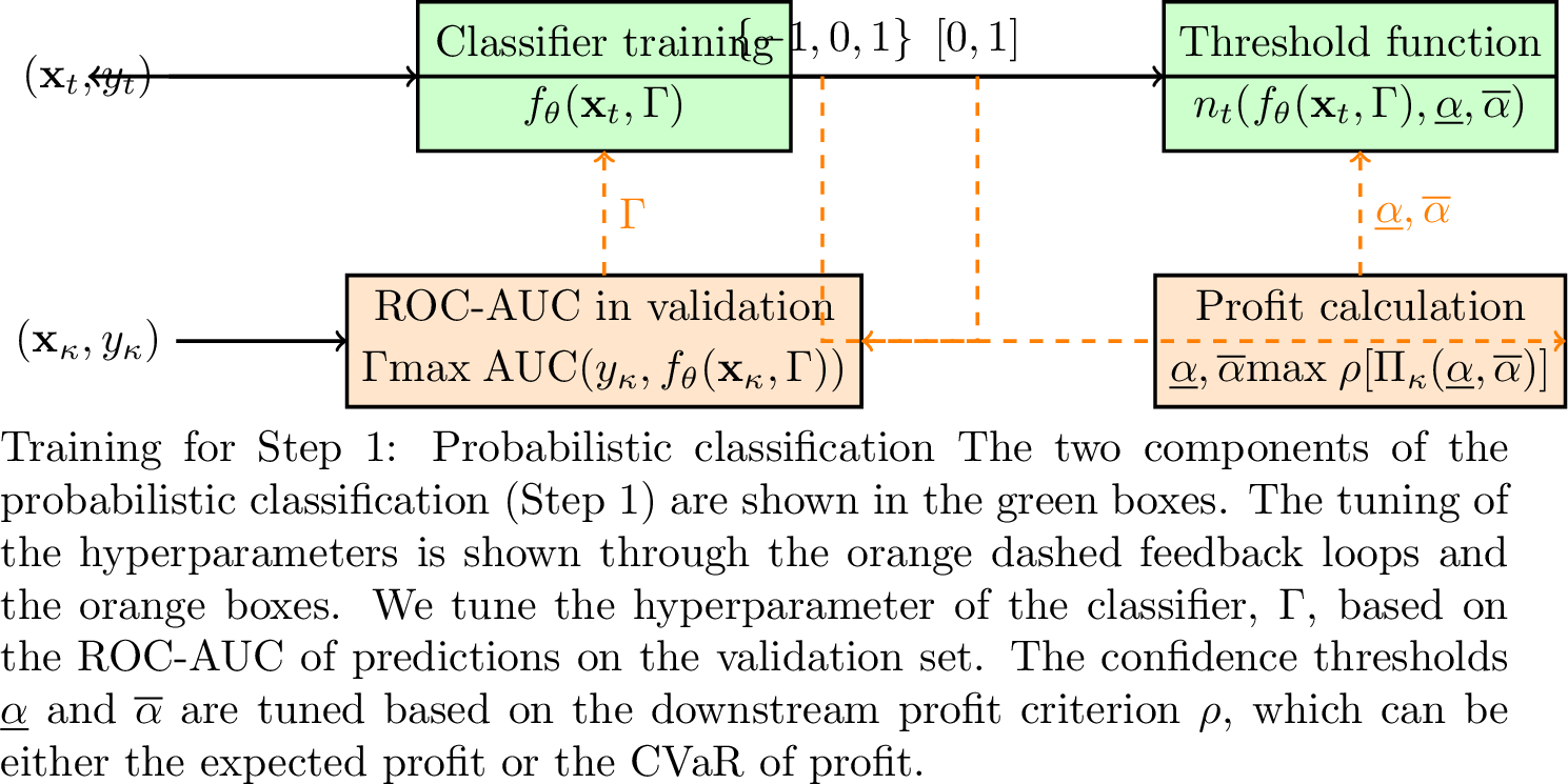In the first model step, a probabilistic binary classifier is trained to predict the sign of the price spread \(\Delta\lambda_t = \lambda^{\rm DA}_t - \lambda^{\rm B}_t\). As established in Section 2.2, the sign of \(\Delta\lambda_t\) is mainly driving the direction of the arbitrage decision. The training procedure is illustrated in Figure 4.

The probabilistic classification is performed based on two components (green boxes). The first component (left green box) is a probabilistic binary classifier \(f_{\boldsymbol{\theta}}(\mathbf{x}_t,\boldsymbol{\Gamma}): \mathbb{R}^d \to [0,1]\) that receives the features \(\mathbf{x}_t \in \mathbb{R}^{d}\) of time period \(t \in \mathcal{T^{\rm train}}\) as input and maps them to the binary target \(y_t\), that takes the value \(1\) if \(\Delta\lambda_t > 0\), and \(-1\) if \(\Delta\lambda_t < 0\). Notation \(\boldsymbol{\theta}\) denotes the classifier parameters, which are learned in the training phase, and \(\boldsymbol{\Gamma}\) denotes the classifiers own model hyperparameters that tune its accuracy and regularization. The hyperparameters \(\boldsymbol{\Gamma}\) are tuned by maximizing a performance metric of the out-of-sample validation set denoted by \(\kappa \in \mathcal{T^{\rm val}}\) (left orange box) to find the best hyperparameter configuration of the classifier \(\tilde{\boldsymbol{\Gamma}}\). In our case study, we use the Area Under the Receiver Operating Characteristic (AUC-ROC) as performance metric to select the best hyperparameters, but it is a design choice for the power trader. In addition to the classifier hyperparameters, we introduce a deadband quantile \(\delta\), that selects which training samples enter the classifier based on the absolute magnitude of the price spread \(|\Delta\lambda_t|\). Samples with a near-zero spread, \(|\Delta\lambda_t|\approx 0\), carry essentially no arbitrage value, since the profit is then almost independent of the bidding decision, while at the same time their labels are the most noise-sensitive, because an arbitrarily small perturbation flips the sign. We remove these low-value, high-noise samples by introducing a central deadband around zero from the classifier training set by dropping the fraction \(\delta\) of training samples with the smallest absolute spread, \[\label{eq:deadband} \mathcal{T}^{\rm train}_{\delta} = \bigl\{\, t \in \mathcal{T}^{\rm train} : |\Delta\lambda_t| > Q_\delta \,\bigr\},\tag{7}\] where \(Q_\delta\) denotes the \(\delta\)-quantile of the absolute spread \(|\Delta\lambda|\) over the training set (\(\delta=0\) recovers the full training set).

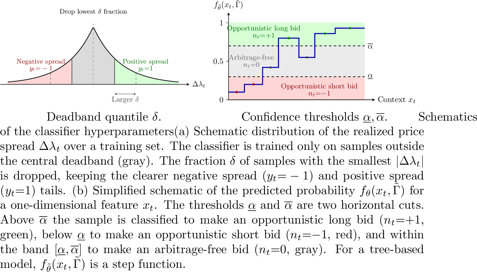Figure [fig:deadband] illustrates in a schematic how the training set shrinks as \(\delta\) grows. The deadband quantile \(\delta\) is also tuned to maximize the ROC-AUC on the validation set, i.e., it is searched over a common grid with \(\boldsymbol{\Gamma}\).

Using the trained classifier with the best hyperparameter configuration \(\tilde{\boldsymbol{\Gamma}}\) and \(\tilde{\delta}\), we introduce two confidence thresholds \(\underline{\alpha} \in [0, 0.5]\) and \(\overline{\alpha} \in [0.5, 1]\) as second component (right green box) to make the final probabilistic classification. This allows us to control the confidence of the final prediction separately for long and short bids. The predicted class \(n_t \in \{-1, 0, 1\}\) is then determined by \[\label{eq:threshold95rule} n_t = \begin{cases} \phantom{-}1 & \text{if } f_{\boldsymbol{\theta}}(\mathbf{x}_t,\tilde{\boldsymbol{\Gamma}}) \geq \overline{\alpha}, \\ -1 & \text{if } f_{\boldsymbol{\theta}}(\mathbf{x}_t,\tilde{\boldsymbol{\Gamma}}) \leq \underline{\alpha}, \\ \phantom{-}0 & \text{otherwise,} \end{cases}\tag{8}\] where \(n_t = 1\) corresponds to make an opportunistic long bid (e.g.,bid maximum in the day-ahead market), \(n_t = -1\) to make an opportunistic short bid (e.g.,bid minimum), and \(n_t = 0\) to make an arbitrage-free bid. Geometrically, as illustrated in a simplified schematic for a single feature \(x_t\) (one-dimensional) in Figure [fig:alpha95thresholds], the thresholds are two horizontal cuts through the learned probability function. The thresholds \(\underline{\alpha}\) and \(\overline{\alpha}\) tune the trade-off between arbitrage exploitation and confidence and can be asymmetric, so the trader can demand different confidence levels for opportunistic long and short bids. When \(\underline{\alpha} = \overline{\alpha} = 0.5\) every sample is assigned an opportunistic bid, i.e., there is no arbitrage-free bids. As \(\underline{\alpha}\) decreases toward \(0\) and \(\overline{\alpha}\) increases toward \(1\), the amount of arbitrage-free bids increases, reducing the exploitation rate of opportunistic bids but improving their confidence.

Since the values of \(\underline{\alpha}\) and \(\overline{\alpha}\) determine which samples enter the policy optimization in Step 2, they are not tuned to minimize the classification loss but value-orientated instead, i.e., to maximize a measure \(\rho\) of the profit, which could be the expectation or CVaR measure, on the validation set (right orange box): \[\underset{\underline{\alpha}, \overline{\alpha}}{\max}\;\rho\!\left[\Pi_\kappa(\underline{\alpha}, \overline{\alpha})\right],\] where \(\Pi_\kappa(\underline{\alpha}, \overline{\alpha})\) is the realized profit on the validation set, \(\kappa \in \mathcal{T^{\rm val}}\), for the given confidence thresholds \(\underline{\alpha}\) and \(\overline{\alpha}\). It is calculated using the optimization model from Section 3.2, that is trained on the training set and then yields the out-of-sample bidding decisions for the validation set. Using these bidding decisions, we can calculate the final profit of the validation set as it will be described in Section 4.1. Depending on the risk preference of the decision maker, \(\rho\) is either the expectation \(\mathbb{E}[\Pi_\kappa(\underline{\alpha}, \overline{\alpha})]\) or the conditional value at risk \(\text{CVaR}[\Pi_\kappa(\underline{\alpha}, \overline{\alpha})]\) of profit, which penalizes large losses in the tail of the profit distribution.

3.2 Optimization↩︎

Given the predicted class \(n_t \in \{-1, 0, 1\}\) from Step 1, we introduce a contextual optimization model (Policies) as Step 2 that translate the prediction into a day-ahead bid \(p_t^{\rm DA}\) to maximize the profit. The model can be configured for different assets. We focus here on a standalone wind farm (wind-only) and a HPP consisting of a co-located wind farm and electrolyzer.

Similar to [16], we learn a linear decision policy \(\pi(n_t,x_t)\) that maps the features \(x_t\) to the bidding decision, instead of fixing the bid at a boundary value. However, unlike [16], we learn two separate policies, one for the long and one short classes, i.e., for \(n_t=1\) and \(n_t=-1\). In our case, the optimal decision \(p_t^{\rm DA}\) is the deviation from the point forecast, i.e., the day-ahead bid is parameterized as \[\label{eq:policy} p_t^{\rm DA} = \hat{P}_t^{\rm W} + z_t, \qquad z_t = \pi(n_t,\mathbf{x}_t) = \mathbf{q}_{n_t}\, \mathbf{x}_t^\top,\tag{9}\] where \(\mathbf{q}_{n_t} \in \mathbb{R}^{|\mathbf{x_t}|}\) is a class-specific parameter vector. The two vectors, \(\mathbf{q}_{-1}\) and \(\mathbf{q}_1\), are learned simultaneously by solving the optimization program shown below over the training set \(\mathcal{T}^{\rm train}\). For the HPP case it reads as follows:

\[\tag{10} \begin{align} \max_{\substack{z_t,\, p_t^{\rm DA},\, p_t^{\rm B},\, p_t^{\rm H},\\ h_t,\, \mathbf{q}_{n_t},\, \xi_t,\, \zeta}} \quad & \frac{\beta}{T} \sum_{d \in \mathcal{T}^{\rm train}} \sum_{t \in \mathcal{T}^{\rm train}(d)} \left( p_t^{\rm DA}{\lambda}_t^{\rm DA} + p_t^{\rm B}{\lambda}_t^{\rm B} + h_t{\lambda}^{\rm H} \right) \nonumber \\ & \quad + (1-\beta) \left( \zeta - \frac{1}{T\epsilon} \sum_{d \in \mathcal{T}^{\rm train}} \sum_{t \in \mathcal{T}^{\rm train}(d)} \xi_t \right) \tag{11} \\ \text{s.t.}\quad & (\ref{eq:policy}) && \forall d,t \nonumber \\ & P_t^{\rm W} = p_t^{\rm DA} + p_t^{\rm B} + p_t^{\rm H} && \forall d,t \tag{12} \\ & -\overline{P}^{\rm H} \le p_t^{\rm DA} \le \overline{P}^{\rm W} && \forall d,t \tag{13} \\ & \underline{P}^{\rm H} \le p_t^{\rm H} \le \overline{P}^{\rm H} && \forall d,t \tag{14} \\ & h_t \le A_s p_t^{\rm H} + B_s && \forall s,d,t \tag{15} \\ & \sum_{t \in \mathcal{T}^{\rm train}(d)} h_t \ge \underline{H} && \forall d \tag{16} \\ & z_t \le 0 && \forall d,t : n_t = -1 \tag{17} \\ & z_t \ge 0 && \forall d,t : n_t = 1 \tag{18} \\ & z_t = 0 && \forall d,t : n_t = 0 \tag{19} \\ & \xi_t \ge \zeta - \left( p_t^{\rm DA}{\lambda}_t^{\rm DA} + p_t^{\rm B}{\lambda}_t^{\rm B} + h_t\lambda^{\rm H} \right) && \forall d,t \tag{20} \\ & \xi_t \ge 0 && \forall d,t \tag{21} \end{align}\]

The optimization program 10 is a linear program that learns the class-specific policy parameters \(\mathbf{q}_{n_t}\) across the full training period. The objective 11 maximizes a weighted combination of the mean profit and the CVaR\(_\epsilon\) of the profit , following the Rockafellar–Uryasev formulation [22], for all days \(d\) in the training period. The first term averages the profit from the day-ahead market, the balancing market, and hydrogen sales across all training periods, using the realized prices \({\lambda}_t^{\rm DA}\), \({\lambda}_t^{\rm B}\), and \({\lambda}^{\rm H}\). The second term, \(\zeta - \frac{1}{T\epsilon}\sum_{d,t}\xi_t\), is the CVaR\(_\epsilon\) of the profit, i.e., the expected profit in the worst \(\epsilon\) fraction of training periods, where \(\epsilon \in [0,1]\) is the tail probability and \(T\) is the total number of samples of the training period. The scalar \(\beta \in [0,1]\) is the weight on the objective terms. Pure profit maximization is achieved by \(\beta = 1\), while smaller values of \(\beta\) shift the weight toward the tail risk of the profit distribution. Constraint 12 is the power balance between the realized wind production \(P_t^{\rm W}\), the day-ahead bid \(p_t^{\rm DA}\), the balancing position \(p_t^{\rm B}\), and the electrolyzer consumption \(p_t^{\rm H}\). Constraint 13 bounds the day-ahead bid. The upper bound \(\overline{P}^{\rm W}\) represents the maximum available wind capacity, while the lower bound \(-\overline{P}^{\rm H}\) allows the HPP to procure electricity from the grid via the day-ahead market to feed the electrolyzer when it is economically favorable. Constraint 14 restricts the power consumption of the electrolyzer to its operational range \([\underline{P}^{\rm H}, \overline{P}^{\rm H}]\), where \(\underline{P}^{\rm H}\) is the minimum stable load required by the device. Constraint 15 represents a piecewise linear approximation of the non-linear production curve of the electrolyzer following [27]. The produced hydrogen \(h_t\) is bounded from above by linear segments \(s\) with slopes \(A_s\) and intercepts \(B_s\). Constraint 16 imposes a minimum daily hydrogen production \(\underline{H}\) aggregated over all delivery periods of each day \(d\), reflecting a contractual offtake obligation or operational target. As given by 9 , the day-ahead bid is parameterized as the wind power forecast \(\hat{P}_t^{\rm W}\) plus a signed deviation \(z_t\), where \(z_t\) is the output of the class-specific linear policy, i.e., the inner product of the parameter vector \(\mathbf{q}_{n_t}\) and the transposed feature vector \(\mathbf{x}_t^\top\). Constraints 17 –19 enforce the directional intent of the classifier for each class: \(z_t \leq 0\) for opportunistic short bids (\(n_t = -1\)), \(z_t \geq 0\) for opportunistic long bids (\(n_t = 1\)) and \(z_t = 0\) for arbitrage-free bids (\(n_t = 0\)), i.e., bidding exactly the wind power forecast. Together, these three constraints ensure that the learned policies never contradict the classification from Step 1. Finally, constraints 20 –21 implement the CVaR\(_\epsilon\) auxiliary variables following [22]. The auxiliary variable \(\xi_t\) in 20 captures the shortfall of the profit below the value-at-risk level \(\zeta\). Constraint 21 enforces the non-negativity of \(\xi_t\), ensuring that only downside deviations contribute to the tail penalty. The value-at-risk level \(\zeta\) is a free variable optimized jointly with the policy parameters, and the CVaR expression in the objective is concave in \(\zeta\), preserving the linearity of the overall program.

For the wind-only case, the contextual optimization problem simplifies in four ways: (i) the hydrogen revenue term \(h_t{\lambda}^{\rm H}\) is dropped from both the profit sums in the objective 11 and the CVaR auxiliary constraint 20 , (ii) the power balance 12 reduces to \(P_t^{\rm W} = p_t^{\rm DA} + p_t^{\rm B}\), (iii) the lower bound on the day-ahead bid in 13 tightens from \(-\overline{P}^{\rm H}\) to \(0\), since there is no electrolyzer to consume grid power, and (iv) the electrolyzer constraints 14 –16 are removed entirely. All remaining constraints are identical to the HPP formulation.

4 Testing↩︎

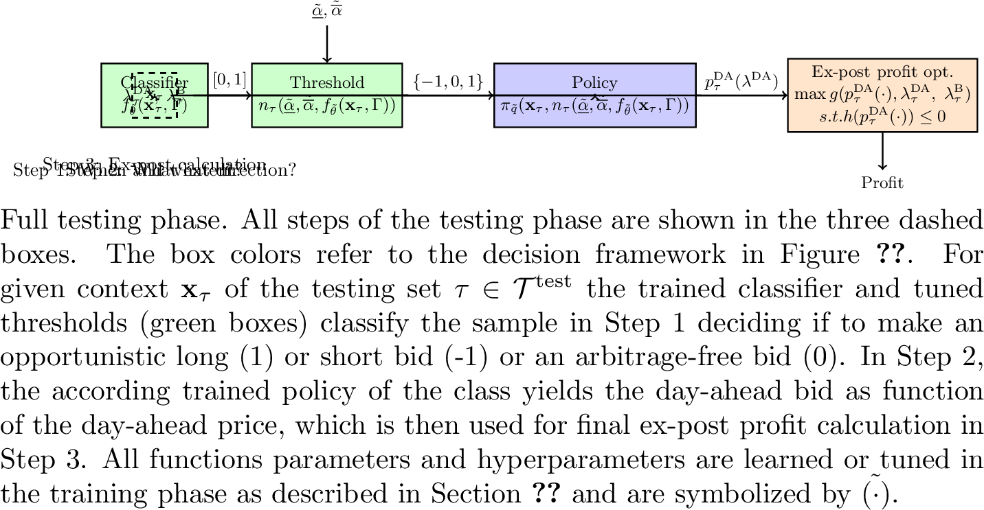The testing phase applies the fully trained model to unseen test periods \(\tau \in \mathcal{T}^{\rm test}\), as illustrated in Figure 6. At each test period \(\tau\), the contextual feature vector \(\mathbf{x}_\tau\), available at gate closure of the day-ahead market, is processed sequentially through three steps. All model parameters and hyperparameters \(\tilde{\mathbf{q}}\), \(\tilde{\boldsymbol{\theta}}\), \(\tilde{\delta}\), \(\tilde{\boldsymbol{\Gamma}}\), \(\tilde{\underline{\alpha}}\), \(\tilde{\overline{\alpha}}\) are fixed at the values determined during the training phase and are not updated during the testing phase.

4.0.0.1 Step 1: When and what direction?

The trained classifier \(f_{\tilde{\boldsymbol{\theta}}}(\mathbf{x}_\tau, \tilde{\boldsymbol{\Gamma}})\) maps the features to a predicted probability \(\hat{p}_\tau \in [0,1]\) that \(\Delta\lambda_\tau > 0\). Applying the tuned confidence thresholds \(\tilde{\underline{\alpha}}\) and \(\tilde{\overline{\alpha}}\) as described in Section 3.1, the threshold function assigns the predicted class \(n_\tau \in \{-1, 0, 1\}\): \(n_\tau = 1\) (opportunistic long bid), \(n_\tau = -1\) (opportunistic short bid), or \(n_\tau = 0\) (arbitrage-free bid).

4.0.0.2 Step 2: What extent?

Given \(n_\tau\), the corresponding trained linear policy \(z_\tau=\pi_{\tilde{\mathbf{q}}}(n_\tau,\mathbf{x}_\tau) = \tilde{\mathbf{q}}_{n_\tau} \mathbf{x}_\tau^\top\) yields the signed deviation \(z_\tau\), and the final day-ahead bid follows from \(p_\tau^{\rm DA} = \hat{P}_\tau^{\rm W} + z_\tau\), as in 9 . If the resulting bid violates the physical bounds, it is projected to the nearest feasible point.

4.0.0.3 Step 3: Profit evaluation.

With \(p_\tau^{\rm DA}\) committed, the realized day-ahead and balancing prices \(\lambda_\tau^{\rm DA}\) and \(\lambda_\tau^{\rm B}\) become available ex-post. The profit is calculated as described in Section 4.1, where the procedure differs between the wind-only and HPP cases.

4.1 Profit Evaluation↩︎

Once the day-ahead bid \(p_\tau^{\rm DA}\) is committed in Step 2, the profit in Step 3 is computed differently depending on whether the asset is a standalone wind farm or an HPP. Note, that we assume that the day-ahead price can be forecasted well, i.e., if prices become negative, we adjust the day-ahead bid to its minimum, i.e., \(p^{\rm DA}=0\) (wind-only) or \(p^{\rm DA}=-\overline{P}^{\rm H}\) (HPP), which reflects the pragmatic decision of a power trader in case of negative day-ahead prices. As this adjustment is made for all models including the benchmarks, this is equivalent to removing the samples with negative day-ahead prices.

4.1.0.1 Wind-only case.

For a standalone wind farm, no further operational decision is required after the day-ahead bid is submitted. Any deviation between the realized wind production \(P_\tau^{\rm W}\) and the committed bid is automatically settled in the balancing market, so the balancing deviation and profit follow directly as \[p_\tau^{\rm B} = P_\tau^{\rm W} - p_\tau^{\rm DA}, \qquad \Pi_\tau = \lambda_\tau^{\rm DA}\, p_\tau^{\rm DA} + \lambda_\tau^{\rm B}\, p_\tau^{\rm B}.\]

4.1.0.2 HPP case.

For the HPP, committing the day-ahead bid \(p_\tau^{\rm DA}\) leaves a residual wind power quantity that must be allocated between the electrolyzer and the balancing market. Since the electrolyzer can be actively dispatched before physical delivery, its consumption is determined by solving a deterministic linear program using the balancing price forecast \(\hat{\lambda}_\tau^{\rm B}\) and the wind power forecast \(\hat{P}_\tau^{\rm W}\), both available before delivery: \[\tag{22} \begin{align} \max_{p_\tau^{\rm B},\, p_\tau^{\rm H},\, h_\tau} \quad & \sum_{\tau} \left( \hat{\lambda}_\tau^{\rm B}\, p_\tau^{\rm B} + \lambda^{\rm H} h_\tau \right) \tag{23}\\ \text{s.t.} \quad & p_\tau^{\rm B} + p_\tau^{\rm H} = \hat{P}_\tau^{\rm W} - p_\tau^{\rm DA} && \forall\,\tau \tag{24}\\ & \underline{P}^{\rm H} \le p_\tau^{\rm H} \le \overline{P}^{\rm H} && \forall\,\tau \tag{25}\\ & h_\tau \le A_s\, p_\tau^{\rm H} + B_s && \forall\,s,\tau \tag{26}\\ & \textstyle\sum_{\tau \in \mathcal{T}(d)} h_\tau \ge \underline{H} && \forall\,d. \tag{27} \end{align}\] The objective 23 maximizes the sum of balancing revenue and hydrogen sales revenue, using the forecasted balancing price \(\hat{\lambda}_\tau^{\rm B}\) and the fixed hydrogen price \(\lambda^{\rm H}\). The power balance 24 allocates the forecast residual between electrolyzer consumption \(p_\tau^{\rm H}\) and balancing deviation \(p_\tau^{\rm B}\). Constraints 25 and 26 enforce the electrolyzer’s operational bounds and the piecewise linear hydrogen production efficiency, identical to the training constraint 10 . Constraint 27 enforces the minimum daily hydrogen production \(\underline{H}\).

Given the optimal dispatch \((p_\tau^{\rm B*},\, p_\tau^{\rm H*},\, h_\tau^*)\), the corresponding realized profit is \[\Pi_\tau = \lambda_\tau^{\rm DA}\, p_\tau^{\rm DA} + \lambda_\tau^{\rm B}\, p_\tau^{\rm B*} + \lambda^{\rm H} h_\tau^*.\] Note that while the electrolyzer dispatch is optimized against the forecasted balancing price \(\hat{\lambda}_\tau^{\rm B}\), the balancing revenue is settled ex-post at the realized price \(\lambda_\tau^{\rm B}\).

5 Numerical Results↩︎

This section presents a numerical analysis of the proposed framework. All source code is publicly available in [28].

5.1 Case Studies↩︎

5.1.0.1 Data.

Our case study considers two European market bidding zones, DK1 (Denmark) and DE/LU (Germany/Luxembourg), and two portfolio cases, a standalone wind farm (wind-only) and a co-location with an electrolyzer (HPP). Performance is evaluated via rolling-window as illustrated in Figure 3. The data considered for these studies ranges from April 2025 to February 2026. Since the data exists on different resolutions (60min and 15min), we average the data to 60min resolution. The physical asset is a real 7.2MW wind farm (\(\overline{P}^{\rm W}=7.2\)MW) with a point-forecast \(\hat{P}^{\rm W}\), optionally coupled with an electrolyzer of half the wind farm capacity (\(\overline{P}^{\rm H}=3.6\)MW). The hydrogen price is set to €2/kg and the electrolyzer minimum stable load to 10% of its rated capacity. The hydrogen production efficiency curve is approximated with two linear segments following the HYP-L method of [27]. A minimum daily hydrogen production of 100kg (approximately 5MWh of electrolyzer energy consumption) is enforced.

Each rolling window uses a 7-day test period (models are retrained weekly), a 4-month training set, and a 1-month validation set, yielding 22 windows in total. A dataset consisting of 200+ features is created using publicly available data from Entso-e, Energinet and Open-Meteo including lagged and forecasted data of relevant energy markets and weather. A full overview of the features in each category is given in Appendix A. All features are z-score normalized. Feature selection is performed on each rolling window using SHAP importance values, that selects only features with an importance above 0.6.

5.1.0.2 Classification.

In the training phase of the classifier we ignore the data with zero price spread, as no arbitrage is possible in these cases, i.e., the profit is independent of the day-ahead bidding decision, and they only add additional noise to the model. For each model, hyperparameters are selected by grid search on the validation set using the ROC-AUC as the criterion. The deadband quantile \(\delta\) is tuned over \([0.0,0.8]\). The confidence thresholds are tuned over the grid \(\underline{\alpha} \in \{0.15,\,0.25,\,0.35,\,0.45\}\) and \(\overline{\alpha} \in \{0.55,\,0.65,\,0.75,\,0.85\}\). Having tested different classification models such as statistical, tree-based, and neural network approaches, LightGBM (LGBM) achieves the best out-of-sample classification performance and is used in all subsequent result sections. The model specifications and hyperparameter grid of the LGBM model is given in Appendix B.

5.1.0.3 Model Overview.

We compare our proposed predict-then-contextual-optimize model with 5 benchmarks in the following analysis. All models are summarized in Table ¿tbl:tab:models?. Our proposed Classification + Policies model pairs the Step 1 classifier of Section 3.1 with the Step 2 linear policies models of Section 3.2 learned via contextual optimization.

5.2 Profit Over All Testing Windows↩︎

We start by calculating the profit improvement of our proposed Classification + Policies model in comparison to the simple arbitrage-free bidding strategy of the Bid Forecast model, that always bids the forecasted wind power production into the day-ahead market.

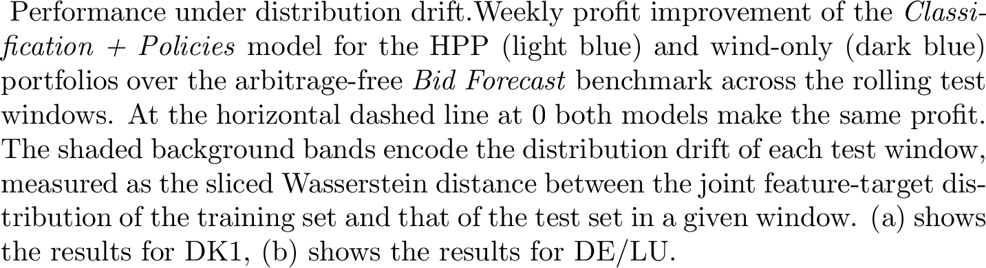Figure 7 shows the out-of-sample profit improvement for the HPP and wind-only portfolios and both markets, DK1 and DE/LU, over all testing windows given a high weight on the mean profit objective term in 11 , \(\beta=0.9\). A positive value reflects the profit that the arbitrage learning adds on top of simply bidding the wind forecast. In addition, the profit improvement is shown in relation to the amount of distribution drift between the training and testing set for each window that is visualized as shaded background band for each window and measured as the sliced Wasserstein distance between the joint feature-target distributions [29], [30].

Across all windows the HPP (light blue) achieves more arbitrage profit than the standalone wind farm (dark blue) in both markets. The reason is the additional internal flexibility provided by the electrolyzer. The electrolyzer can absorb part of the mismatch between the day-ahead bid and the realized wind production internally, which lets the policy place more opportunistic bids with larger magnitude and capture a larger share of the price spread without exposing the portfolio to the full imbalance cost. The HPP improvements therefore peak well above the benchmark (around \(+75\%\) in DK1 and above \(+100\%\) in DE/LU), whereas the wind-only portfolio stays much closer to the benchmark model and seldom shows a profit improvement more than about \(30\%\).

The distribution drift bands explain much of the window-to-window variation in testing. In windows with small drift, where the test distribution still resembles the training data, the classifier and policies generalize better and the arbitrage learning delivers its largest profit improvement. Therefore, most of the pronounced positive spikes coincide with the lighter bands. As the distribution drift grows the profit improvement tends to shrink, and under the most severe drifts (darker red bands) it collapses towards zero or even turns negative, meaning the learned policy can do worse than simply bidding the forecasted wind power production. This is the expected failure when the environment is non-stationary, i.e., the model was trained on a different environment of features and target and the confident opportunistic out-of-sample bids are increasingly placed on the wrong side of the spread. This is most visible for the wind-only case in DK1, where the third window with much larger distribution drift than the surrounding testing windows causes the profit improvement to fall down to around \(-100\%\).

In the following, we limit the analysis to the HPP case and the DK1 market to avoid redundancies. Figure 8 reports the realized per-hour profit distributions over all 22 rolling test windows for the HPP portfolio comparing all models that are defined in Table ¿tbl:tab:models?. For the Classification models (b, d, f), the confidence thresholds are tuned as described in Section 3.1 and \(\beta\) is now set to \(\beta=0.7\) to balance more between both objective terms in 11 . The two hindsight-based models (a,b) bound the achievable performance. Our proposed model Classification + Policies (f) outperforms the Bid Forecast (c) and Single Policy (e) benchmark models in terms of mean profit, however, at a lower CVaR_5% value. The Classification + Policies shows a mean profit that is 7% higher than the Bid Forecast and 4% higher than the Single Policy with a lower CVaR_5% of 19% and 51% respectively. Compared to the Classification + All-or-Nothing it shows a slightly lower mean profit of 3%, while the CVaR_5% is 86% better. This shows, that All-or-Nothing is an extreme case of our proposed Policies model in Step 2 and, therefore, has the heaviest tail of all models but also highest mean profit. The Classification + Policies model, by contrast, retains a comparable mean profit while significantly compressing this tail as its learned policies per class scale the opportunistic bid magnitude with the contextual features instead of committing to the all-or-nothing extremes. Hence, it is capable of finding a balance between a higher mean profit and higher risk (CVaR_5%), which is important especially in non-stationary environments.

5.3 Illustration of Opportunistic Bids↩︎

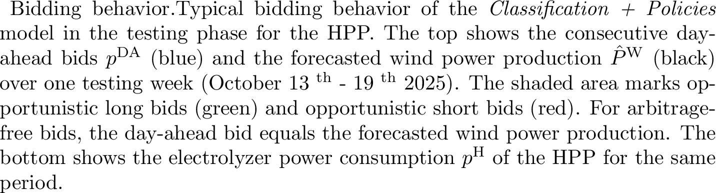Figure 9 illustrates in the upper panel the typical bidding behavior of our proposed Classification + Policies model over a representative test period for the HPP (blue line) in DK1. Whenever the classifier is not confident enough in the sign of the price spread, the policy falls back to the arbitrage-free bid and bids the wind power forecast \(\hat{P}^{\rm W}_t\) (black line). When the classifier is sufficiently confident, the policy instead places an opportunistic bid that differs from the forecast. An opportunistic long bid offers more energy to the day-ahead market than is expected to be produced (green shaded area), anticipating that the balancing price will settle below the day-ahead price, and saturates at the maximum day-ahead capacity \(\overline{P}^{\rm W}=7.2\)MW. An opportunistic short bid offers less than the forecast (red shaded area) to make arbitrage profit on the balancing market. It saturates at the maximum capacity that can be bought in the day-ahead market, which is \(-\overline{P}^{\rm H}=-3.6\)MW for the HPP adding additional flexibility compared to a standalone wind farm that can only offer non-negative bids. Hence, the HPP can make larger short opportunistic bidding decisions to increase the profits. The bottom panel shows the associated electrolyzer dispatch \(p^{\rm H}\), which operates between its minimum power consumption and full power consumption.

5.4 Risk Sensitivity Analysis↩︎

In our framework, two groups of parameters tune the risk exposure of the day-ahead bidding decision and they act on different stages of the pipeline. The first group are the two confidence thresholds \(\underline{\alpha} \in [0,0.5]\) and \(\overline{\alpha} \in [0.5,1]\) of the classification step, which set the classifier confidence required before an opportunistic bid is placed through the threshold rule 8 . They set the risk of making an opportunistic bid, i.e., when and in what direction the trader deviates from the arbitrage-free bid. Lowering \(\underline{\alpha}\) toward \(0\) and raising \(\overline{\alpha}\) toward \(1\) widens the arbitrage-free band and yields fewer, more selective and confident opportunistic bids, whereas pushing both thresholds toward \(0.5\) admits more opportunistic bidding with less confidence. The second group is the single weight \(\beta \in [0,1]\) in the policy objective 11 , which sets the risk of the magnitude of an opportunistic bid. When \(\beta = 1\), the objective is to maximize mean profit solely, while decreasing \(\beta\) shifts weight onto CVaR_5% of the profit and shrinks the tail.

Figure 10 reports the joint out-of-sample effect of both groups for the Classification + Policies model on the HPP portfolio in DK1, showing the CVaR_5% of the profit over all testing windows (top row) and the mean profit (bottom row) over the \(\underline{\alpha} \times \overline{\alpha}\) grid for different values of \(\beta\). The figure shows that both, the mean profit and CVaR_5% value, experience an asymmetric effect of the confidence thresholds, which is, however, larger for the CVaR_5% value. Especially, the upper threshold \(\overline{\alpha}\) appears to be a dominant factor improving CVaR_5% consistently across all values of \(\beta\). The reason is that opportunistic long bids, which offer more energy than is forecast to be produced, are the main source of large imbalance costs when the spread realizes in the opposite direction, and a higher \(\overline{\alpha}\) filters out the least confident of these opportunistic long bids. The lower threshold \(\underline{\alpha}\) behaves the opposite, i.e., allowing more opportunistic short bids with lower confidence (larger \(\underline{\alpha}\)) tends to improve rather than worsen the tail. The mean profit, by contrast, is maximized at a moderate threshold pair (around \(\underline{\alpha}=0.35\) and \(\overline{\alpha}=0.65\)) rather than at either corner. Therefore, the most arbitrage-free configuration misses profitable arbitrage and lowers the mean profit, while the most opportunistic bidding with least confidence configuration adds little mean profit at a significant worse tail.

The weight \(\beta\) in the optimization objective (11 ) shows the mean profit–risk trade-off along the columns of Figure 10. Increasing \(\beta\) raises the mean profit but deepens the tail, i.e., the CVaR_5% becomes more negative. However, this trade-off is strongly asymmetric over the threshold grid. It is mild in the conservative region with few opportunistic bids (top left corner) but severe when many opportunistic long bids with low confidence are admitted (low \(\overline{\alpha}\)), where the worst-case loss roughly doubles between the most risk-averse (\(\beta=0.1\)) and the most profit-seeking (\(\beta=0.9\)) policy. Hence the weight \(\beta\) matters most precisely when the thresholds allow many opportunistic long bids with low confidence, so the two parameter groups interact rather than act independently.

6 Conclusion↩︎

In this paper we studied how a price-taking stochastic energy generator should engage in opportunistic arbitrage between the day-ahead and balancing markets under single-price balancing. We proposed a predict-then-contextual-optimize framework that decomposes the day-ahead bidding decision into three explainable stages to decide, when to engage in arbitrage, in what direction, and to what extent. The first two stages are answered in a first step by a probabilistic classification with two confidence thresholds. A linear decision policy per class is learned in a second step through contextual optimization to determine the magnitude of the deviation from the forecast answering the third stage. The proposed model was tested in two European markets (DK1, DE/LU) for a standalone wind farm and a co-located wind farm and electrolyzer. It showed increased mean profits compared to the benchmark models. Especially, the co-located electrolyzer substantially raised arbitrage profits by providing additional bidding flexibility. The risk sensitivity analysis showed that the two parameter groups, the two confidence thresholds and the single CVaR weight, allow explainable tuning of the profit–risk trade-off, while the distribution drift analysis confirmed that the arbitrage profit improvements concentrate in windows with small drift and decrease under strong distribution drift.

Our study has several limitations that are left for future research. First, the distribution-drift analysis shows that non-stationarity can limit the arbitrage profits achieved by the proposed framework. An online prediction and policy updating scheme could allow the framework to adapt continuously to changing market conditions. Second, this work focuses on the perspective of a single price-taking trader. Studying the market-level implications of opportunistic arbitrage bidding, including its effects on liquidity, price convergence, and social welfare when such strategies are adopted at scale, remains an important direction for future research.

Acknowledgments↩︎

We gratefully acknowledge the Danish Energy Technology Development and Demonstration Programme (EUDP) for supporting this research through the ViPES2X project (Grant number: 640222-496237), and the Innovation Fund Denmark for supporting our work through the PtX Markets project (Grant number: 150-00001B). We are also grateful to Enfor for providing data and Jan Leisbrock and David Miles-Skov for valuable discussions throughout the course of this work.

7 Feature Overview↩︎

Table ¿tbl:tab:app95features? summarizes the feature categories considered in the case study (Section 5.1). The full dataset with all features can be found in [28]. All features are z-score normalized, and feature selection is performed on each rolling window using SHAP importance values.

8 Classification Model and Hyperparameter Grids↩︎

This appendix lists the LGBM classification model evaluated in Section 5.1, including its fixed parameters and the hyperparameter grids searched on the validation set. The model uses balanced class weights to counteract class imbalance.

References↩︎