This work has been submitted to the IEEE for possible publication. Copyright may be transferred without notice, after which this version may no longer be accessible.

1 Introduction↩︎

Hypergraphs provide a natural representation for complex systems involving higher-order relations, where one interaction may simultaneously connect more than two entities. Unlike ordinary pairwise graphs, hypergraphs explicitly encode group-wise dependencies through hyperedges and are therefore well suited for modeling relational patterns in social networks, biological systems, recommendation, and brain network analysis [1]–[4]. Motivated by this expressive capability, hypergraph neural networks (HGNNs) have been developed to extend graph neural message passing from pairwise edges to node–hyperedge incidence structures [5]–[9]. By aggregating information between nodes and hyperedges, these models have achieved promising performance in various prediction tasks.

Despite their empirical success, the predictive reliability of existing HGNNs remains insufficiently explored. Most HGNNs are formulated as deterministic representation learning models: given a hypergraph and node attributes, they produce a single deterministic representation path through stacked propagation layers and a single predictive distribution [5]–[7]. Such deterministic behavior is problematic in high-stakes applications, where a model is expected not only to make accurate predictions but also to indicate when its predictions are unreliable [10], [11]. This issue is particularly important for hypergraph learning, where uncertainty may arise from attribute-level noise, label-space ambiguity, variability in node–hyperedge incidence patterns, and nontrivial dependencies among higher-order interactions. In these cases, an HGNN may produce overconfident predictions even when the underlying higher-order relational context is noisy, ambiguous, or shifted from the training distribution [12], [13].

Uncertainty estimation on hypergraphs presents additional challenges compared with ordinary graphs. Existing graph uncertainty methods mainly focus on uncertainty associated with node attributes, labels, or pairwise edges [12]–[15]. In hypergraphs, however, uncertainty is also coupled with the incidence structure between nodes and hyperedges. Since a hyperedge represents a group-wise relation, modifying one hyperedge can simultaneously change the aggregation contexts of all its incident nodes [2], [5], [6]. Therefore, uncertainty estimation should not be restricted to output-level confidence scores; rather, stochastic representation variability should be modeled along node–hyperedge incidence relations during higher-order message passing. For instance, a distribution-shifted hyperedge structure may alter the representation dynamics of multiple nodes even when their input features remain unchanged. This observation suggests that uncertainty estimation for HGNNs should go beyond output-level confidence and explicitly characterize stochastic variability along node–hyperedge incidence structures.

Existing uncertainty estimation methods are not fully satisfactory for this purpose. Deep ensembles provide strong empirical uncertainty estimates but incur substantial computational and storage costs [11]. Bayesian neural networks offer a principled probabilistic formulation, yet posterior inference or approximation is often expensive and difficult to scale to large relational structures [16]. Deterministic and post-hoc uncertainty methods avoid repeated training or posterior sampling, but they usually estimate uncertainty from final logits or predictive distributions, without modeling how uncertainty propagates during representation learning [10], [17]. Recent graph uncertainty methods have made important progress by considering graph-dependent uncertainty, energy propagation, and stochastic graph diffusion [12]–[15], [18], [19]. However, these methods are primarily developed for pairwise graphs and do not directly address the higher-order incidence mechanism of hypergraphs. Moreover, when hypergraphs are approximated by pairwise graph expansions, the original incidence-level geometry may be distorted or partially lost, making it difficult to model stochastic perturbations directly on node–hyperedge interactions.

In this paper, we propose Hypergraph Neural Stochastic Diffusion (HyperNSD), a stochastic differential equation (SDE) framework for uncertainty estimation on hypergraphs. HyperNSD formulates hypergraph representation learning as a stochastic diffusion process over the node–hyperedge incidence domain. Instead of producing a single deterministic representation trajectory, HyperNSD evolves node representations along multiple structure-informed stochastic paths. The resulting pathwise variability provides a representation-level basis for uncertainty estimation. Specifically, a learnable drift term models deterministic higher-order neural diffusion, while a learnable stochastic forcing term models data-dependent perturbations associated with representation noise and structural ambiguity. Since both terms are defined through the hypergraph gradient operator, the resulting stochastic representation dynamics are explicitly coupled with the node–hyperedge incidence structure. This design embeds uncertainty into the representation dynamics rather than appending it as a post-hoc confidence score, while avoiding multiple independently trained models, complex posterior approximation, or fixed-form output-level priors.

We further provide theoretical guarantees for the proposed HyperNSD, including well-posedness, moment stability, stability with respect to initial-state and structural perturbations, structure-constrained stochastic modes, permutation equivariance, and convergence of the Euler–Maruyama approximation. In practice, HyperNSD is instantiated with neural parameterizations of the drift and stochastic forcing terms, and uncertainty is estimated from the variability of sampled terminal representations and their corresponding predictive distributions. This enables HyperNSD to support out-of-distribution detection and misclassification detection under semantic, attribute-level, and structural distribution shifts. Extensive experiments on multiple hypergraph benchmarks show that HyperNSD consistently improves out-of-distribution (OOD) and misclassification detection across different distribution-shift settings while maintaining competitive in-distribution predictive accuracy. Additional analyses further demonstrate the importance of incidence-aware stochastic forcing, adaptive noise modulation, and direct modeling of the original hypergraph incidence domain.

The main contributions of this paper are summarized here:

• We identify incidence-coupled structural variability as a key challenge for uncertainty estimation on hypergraphs, where stochastic representation variability can be shaped by group-wise node–hyperedge interactions rather than captured solely by output-level confidence.

• We propose Hypergraph Neural Stochastic Diffusion (HyperNSD), an SDE-based framework that unifies deterministic higher-order neural diffusion and learnable stochastic forcing over the node–hyperedge incidence domain.

• We establish theoretical guarantees for HyperNSD, including solution well-posedness, moment stability, stability under initial-state and structural perturbations, and numerical convergence. We further show that the proposed dynamics preserve structure-constrained stochastic modes and are permutation equivariant.

• We conduct extensive experiments under label leave-out, feature interpolation, and structure manipulation settings, demonstrating improved OOD and misclassification detection. Additional ablation, graph-expansion, and perturbation-strength analyses further validate the necessity of incidence-aware stochastic forcing and direct hypergraph-domain modeling.

2 Related Work↩︎

2.1 Hypergraph Neural Networks↩︎

Hypergraph neural networks extend pairwise graph learning to higher-order relational structures by propagating information between nodes and hyperedges. Existing methods can be broadly categorized according to how they construct higher-order message-passing operators. Spectral methods such as HGNN perform convolution based on normalized hypergraph Laplacians, while graph-expansion methods such as HyperGCN approximate each hyperedge using representative pairwise connections [5], [20]. In contrast, node–hyperedge message-passing methods explicitly model interactions between nodes and hyperedges. For example, HNHN maintains and updates both node and hyperedge representations, AllSet formulates node–hyperedge aggregation through learnable multiset functions, and HGNN+ provides a flexible framework for general hypergraph message passing [6], [7], [21], [22]. Unified formulations such as UniGNN further connect graph and hypergraph propagation rules, facilitating the adaptation of established graph architectures to higher-order relational data [23].

Subsequent studies have improved the expressiveness, symmetry, and optimization properties of hypergraph learning. Equivariant architectures preserve permutation symmetries of hypergraph representations, while ED-HNN characterizes a broad class of continuous equivariant hypergraph diffusion operators [24], [25]. Energy-based formulations derive hypergraph neural architectures from learnable regularized energy functions, providing an optimization-oriented interpretation of higher-order representation learning [26]. Recent analyses have also investigated hypergraph-specific homophily, architectural design, transferability, and information bottlenecks such as oversquashing [27]–[29]. Closely related to our formulation, diffusion-based models such as HNDiffN and HND interpret node–hyperedge message passing as continuous or discretized diffusion dynamics, while curvature-guided approaches adapt the diffusion process according to higher-order geometric structures [8], [9], [30]. Despite these advances, existing hypergraph models mainly focus on representation expressiveness, propagation depth, and predictive performance. They are mostly deterministic and do not explicitly model pathwise stochastic variability or uncertainty propagation over node–hyperedge incidence structures.

2.2 Uncertainty Estimation on Graphs↩︎

Predictive uncertainty estimation has been extensively studied through Bayesian neural networks, Monte Carlo dropout, deep ensembles, and confidence-based scoring methods [10], [11], [16], [31]–[35]. In OOD and misclassification detection, these methods typically construct uncertainty scores from logits, predictive entropy, energy values, or feature-space distances. Although effective in many settings, they are primarily designed for independently sampled data and do not explicitly characterize how stochastic variability is shaped by relational structures during representation learning.

For graph-structured data, recent studies incorporate graph dependencies into posterior inference, energy propagation, graph-dependent uncertainty modeling, and stochastic representation dynamics [12], [14], [17], [19]. More closely related to our work, GNSD formulates graph representations as stochastic diffusion processes driven by a \(\mathcal{Q}\)-Wiener process, LGNSDE models latent graph dynamics using Brownian perturbations and parameter uncertainty, and structure-informed graph stochastic differential equations introduce spatially correlated perturbations into graph message passing [13], [15], [18]. Hypergraph OOD generalization methods such as HyperGOOD further consider distribution shifts in hypergraph learning, but they are not designed to estimate predictive uncertainty through stochastic incidence-domain dynamics.

Most existing graph uncertainty methods are constructed on pairwise graph operators and therefore do not directly capture the higher-order propagation geometry induced by node–hyperedge incidence relations. Pairwise graph expansions may also distort or partially lose the original incidence-level geometry of hypergraphs, making it difficult to model stochastic perturbations directly on node–hyperedge interactions. In contrast, HyperNSD defines both deterministic drift and stochastic forcing through incidence-based hypergraph operators. Node-space Wiener perturbations are first mapped to the incidence domain, adaptively modulated according to local node–hyperedge contexts, and then propagated back to the node space. This formulation embeds stochastic variability directly into higher-order representation dynamics and enables predictive uncertainty to be estimated from multiple structure-informed stochastic trajectories.

3 Preliminaries↩︎

3.1 Notations↩︎

Let \(\mathcal{G}=(\mathcal{V},\mathcal{E},\omega)\) be a weighted hypergraph, where \(\mathcal{V}\) is the node set with \(|\mathcal{V}|=n\), \(\mathcal{E}\) is the hyperedge set, and \(\omega:\mathcal{E}\rightarrow \mathbb{R}_{>0}\) assigns a positive weight \(\omega_e\) to each hyperedge \(e\in\mathcal{E}\). Each hyperedge is a subset of nodes, i.e., \(e\subseteq \mathcal{V}\) and \(|e|\geq 2\). For each node \(v\in\mathcal{V}\), its degree is defined as \(d_v=\sum_{e\in\mathcal{E}}\mathbb{I}(v\in e)\), where \(\mathbb{I}(\cdot)\) denotes the indicator function. The node–hyperedge incidence set is denoted by \(\mathcal{I}=\{(e,v)\mid e\in\mathcal{E}, v\in e\},\) with \(|\mathcal{I}|=N=\sum_{e\in\mathcal{E}}|e|\).

The node degree matrix \(\mathbf{D_v} \in \mathbb{R}^{n \times n}\) is defined by \(\mathbf{D_v}({v,v})=d_v\). Let \(\mathbf{\Omega}_{\mathcal{I}}=\operatorname{diag}(\omega_e)_{(e,v)\in\mathcal{I}}\in\mathbb{R}^{N\times N}\) be the incidence-level weight matrix, the input matrix of all nodes is denoted as \(\mathbf{X}_{\text{init}}\), and \(\|\cdot\|_F\) denotes the Frobenius norm. We introduce two finite-dimensional Hilbert spaces. The node function space is \(L(\mathcal{V}) := \{\mathbf{f}: \mathcal{V} \to \mathbb{R}^d \} \cong \mathbb{R}^{n\times d}\) and the hyperedge–node pair function space is \(L(\mathcal{E}, \mathcal{V}) := \{ \mathbf{g}: \mathcal{I} \to \mathbb{R}^d \} \cong \mathbb{R}^{N\times d}\), where \(d\) denotes the embedding dimension.

3.2 Hypergraph Neural Diffusion↩︎

Following the hypergraph neural differential formulation in [8], we recall the deterministic diffusion operator used as the backbone of our model. Given a hypergraph \(\mathcal{G}=(\mathcal{V},\mathcal{E},\omega)\), the gradient operator maps node signals to incidence-level variations between nodes and hyperedges, while the divergence operator aggregates incidence-level flows back to nodes.

For a node function \(\mathbf{f}\in L(\mathcal{V})\), its gradient over the incidence pair \((e,v)\in\mathcal{I}\) is defined as \[(\nabla \mathbf{f})(e,v)= \frac{\mathbf{f}(v)}{\sqrt{d_v}} - \frac{1}{|e|} \sum_{u \in e} \frac{\mathbf{f}(u)}{\sqrt{d_u}} . \label{eq:hypergraph95gradient}\tag{1}\] The corresponding divergence operator is defined as \[\label{eq:divergence} (\operatorname{div} \mathbf{g})(v) = \sum_{e \ni v}\frac{\omega_e}{\sqrt{d_v}}\left( \mathbf{g}(e, v) - \frac{1}{|e|} \sum_{u \in e} \mathbf{g}(e, u)\right).\tag{2}\]

Based on these operators, the deterministic hypergraph neural diffusion equation can be written as \[\frac{\partial \mathbf{X}(t)}{\partial t}=-\operatorname{div} \left[\mathbf{A}_{\theta}(\mathbf{X}(t))\nabla \mathbf{X}(t) \right], \label{eq:deterministic95hypergraph95diffusion}\tag{3}\] where \(\mathbf{X}(t)\in L(\mathcal{V})\) denotes the time-dependent node representation, and \(\mathbf{A}_{\theta}(\mathbf{X}(t))\in\mathbb{R}^{N\times N}\) is a learnable diagonal modulation operator defined on the incidence space. Its diagonal entry associated with \((e,v)\) controls the diffusion strength between node \(v\) and hyperedge \(e\): \[\mathbf{A}_{\theta}(\mathbf{X}(t))=\operatorname{diag} \left(a_{\theta}(\mathbf{X}_v(t),\mathbf{X}_e(t)) \right)_{(e,v)\in\mathcal{I}}\in\mathbb{R}^{N\times N}, \label{eq:modulation95operator}\tag{4}\] where \(\mathbf{X}_v(t)\) denotes the node representation of node \(v\), and \(\mathbf{X}_e(t)\) denotes an aggregation of node representations within hyperedge \(e\). In matrix form, Eq. 3 becomes

\[\frac{\partial \mathbf{X}(t)}{\partial t}=-\mathbf{G}^{\top}\mathbf{A}_{\theta}(\mathbf{X}(t))\mathbf{G} \mathbf{X}(t). \label{eq:G95matrix95hypergraph95diffusion}\tag{5}\] Here, \(\mathbf{G}\in\mathbb{R}^{N\times n}\) encodes the node–hyperedge incidence structure, and \(\mathbf{G}^{\top}\in\mathbb{R}^{n\times N}\) maps the resulting flows back to the node domain.

3.3 Uncertainty Source↩︎

Predictive uncertainty can be decomposed into aleatoric uncertainty (due to inherent data randomness) and epistemic uncertainty (due to uncertainty in model parameters) [31], [36], [37]. Given a training dataset \(\mathcal{D}\) and a hypergraph \(\mathcal{G}\), the predictive distribution of the target \(\mathbf{y}\) is given by marginalizing over model parameters \(\boldsymbol{\Theta}\): \[\label{eq:bayes95pred} \mathbb{P}(\mathbf{y} \mid \mathcal{G},\mathcal{D}) = \int \mathbb{P}(\mathbf{y} \mid \boldsymbol{\Theta}, \mathcal{G}) \, \mathbb{P}(\boldsymbol{\Theta} \mid \mathcal{D}) \, \mathrm{d} \boldsymbol{\Theta}.\tag{6}\]

The total uncertainty is measured by the entropy of the marginal predictive distribution:

\[\mathcal{H}\left[ \mathbb{E}_{\mathbb{P}(\boldsymbol{\Theta} \mid \mathcal{D})} \left[\mathbb{P}(\mathbf{y} \mid \boldsymbol{\Theta}, \mathcal{G}) \right] \right].\] where \(\mathcal{H}\) denotes the Shannon’s entropy of a probability distribution. Aleatoric uncertainty is commonly characterized by the posterior expectation of the conditional predictive entropy: \[\mathbb{E}_{\mathbb{P}(\boldsymbol{\Theta} \mid \mathcal{D})} \left[ \mathcal{H}\left[\mathbb{P}(\mathbf{y} \mid \boldsymbol{\Theta}, \mathcal{G}) \right] \right].\] Epistemic uncertainty, reflecting uncertainty in model parameters, is the difference between the total and aleatoric uncertainties. It can also be interpreted as the mutual information between the prediction \(\mathbf{y}\) and the parameters \(\boldsymbol{\Theta}\) [38], [39]: \[\label{eq:mutual95info} \begin{align} I(\mathbf{y}, \boldsymbol{\Theta} \mid \mathcal{G}, \mathcal{D}) = \mathcal{H}\left[ \mathbb{E}_{\mathbb{P}(\boldsymbol{\Theta} \mid \mathcal{D})} \left[\mathbb{P}(\mathbf{y} \mid \boldsymbol{\Theta}, \mathcal{G}) \right] \right] \\- \mathbb{E}_{\mathbb{P}(\boldsymbol{\Theta} \mid \mathcal{D})} \left[ \mathcal{H}\left[\mathbb{P}(\mathbf{y} \mid \boldsymbol{\Theta}, \mathcal{G}) \right] \right]. \end{align}\tag{7}\]

4 Methodology↩︎

This section introduces the proposed Hypergraph Neural Stochastic Diffusion (HyperNSD) framework. We first formulate its incidence-aware deterministic drift and stochastic forcing, and then analyze its well-posedness, moment stability, stability under initial-state and structural perturbations, structure-constrained stochastic modes, permutation equivariance, and numerical convergence. Finally, we present the Euler–Maruyama discretization, uncertainty estimation strategy, training objective, and computational complexity.

4.1 Hypergraph Neural Stochastic Diffusion↩︎

4.1.1 General Formulation↩︎

The general form of the proposed hypergraph stochastic diffusion equation (HSDE) is defined as \[\mathrm d\mathbf{X}(t)=\mathbf{F}(\mathbf{X}(t))\mathrm dt+\boldsymbol{\Sigma}(\mathbf{X}(t))\mathrm d\mathbf{Z}(t), \label{eq:general95hsde}\tag{8}\] subject to an initial condition \(\mathbf{X}(0)\), where \(\mathbf{X}(t)\in L(\mathcal{V})\) denotes the stochastic node state at time \(t\). The drift field \(\mathbf{F}:L(\mathcal{V})\rightarrow L(\mathcal{V})\) governs the deterministic hypergraph diffusion dynamics. The stochastic diffusion operator \(\boldsymbol{\Sigma}(\mathbf{X}):L(\mathcal{E},\mathcal{V})\rightarrow L(\mathcal{V})\) determines how stochastic perturbations defined on node–hyperedge incidence relations are propagated to the node state space. The driving process \(\mathbf{Z}(t)\) is an \(L({\mathcal{E},\mathcal{V}})\)-valued \(\mathcal{Q}\)-Wiener process [40]. A formal definition of the \(\mathcal{Q}\)-Wiener process is provided in Appendix 7. The covariance operator \(\mathcal{Q}: L(\mathcal{E},\mathcal{V}) \rightarrow L(\mathcal{E},\mathcal{V})\), specified below, characterizes the correlation structure of stochastic perturbations across node–hyperedge incidence relations.

4.1.2 Hypergraph Neural Drift↩︎

We employ the deterministic hypergraph neural diffusion equation [8] introduced in Section III as the drift component of the proposed stochastic dynamics. Specifically, the drift field \(\mathbf{F}(\mathbf{X}(t))\) is defined as \[\mathbf{F}^{\theta}(\mathbf{X}(t))=-{\mathbf{G}}^{\top} \mathbf{A}_{\theta}(\mathbf{X}(t)) \mathbf{G} \mathbf{X}(t), \label{eq:hsde95drift}\tag{9}\] where \(\mathbf{A}_{\theta}(\mathbf{X}(t))=\operatorname{diag}\big(a_{\theta}(\mathbf{X}_v(t),\mathbf{X}_e(t))\big)_{(e,v)\in\mathcal{I}}\in\mathbb{R}^{N\times N}\) is a learnable diagonal modulation matrix defined over the node–hyperedge incidence set \(\mathcal{I}\).

For each incidence pair \((e,v)\in\mathcal{I}\), let \(\mathbf{X}_e(t)=\operatorname{Agg}_u(\{\mathbf{X}_u(t) : u \in e\})\), where \(\operatorname{Agg}\) is a permutation-invariant aggregator (e.g., mean or max). Then an unnormalized compatibility score is computed as \[\begin{align} &r^{\theta}_{(e,v)} = \sigma\left(\operatorname{MLP}_{\theta}(\mathbf{X}_v(t) \| \mathbf{X}_e(t))\right),\\ &a_\theta(\mathbf{X}_v(t), \mathbf{X}_e(t))= \frac{\exp\big(r^{\theta}_{(e,v)}\big)}{\sum_{e' \ni v} \exp\big( r^{\theta}_{(e',v)} \big)}, \end{align}\] where \(\|\) denotes concatenation, and \(\sigma\) is a \(\operatorname{LeakyReLU}\) activation function. This formulation guarantees that \(a_\theta(\mathbf{X}_v(t), \mathbf{X}_e(t)) > 0\) and \(\sum_{e \ni v} a_\theta(\mathbf{X}_v(t), \mathbf{X}_e(t)) = 1\). This parametrization enables the drift operator to assign incidence-specific drift modulation weights by comparing each node representation with the aggregated representation of its incident hyperedges. Consequently, the deterministic diffusion process adapts to the local node–hyperedge feature configuration while preserving bounded and normalized modulation coefficients.

4.1.3 Hypergraph Neural Stochastic Forcing↩︎

We introduce a \(L(\mathcal{V})\)-valued standard Wiener process \[\mathbf{W}(t)=[\mathbf{W}_{1}(t),\ldots,\mathbf{W}_d(t)]\in L(\mathcal{V}),\] where \(\mathbf{W}_\ell(t)\) are mutually independent \(n\)-dimensional standard Wiener processes. Thus, \(\mathbf{W}(t)\) represents stochastic perturbations defined on hypergraph nodes.

To incorporate the hypergraph incidence geometry into the stochastic forcing, we transform the node-space Brownian motion through the hypergraph gradient: \[\mathbf{Z}(t)=\mathbf{G}\mathbf{W}(t), \label{eq:incidence95wiener}\tag{10}\] Since \(\mathbf{G}\in\mathbb{R}^{N\times n}\) acts independently on each feature dimension, \(\mathbf{Z}(t)\in L(\mathcal{E},\mathcal{V})\) defines a stochastic process over node–hyperedge incidence pairs. Although the node-level perturbations are mutually independent, their transformation through \(\mathbf{G}\) may induce correlations between different incidence pairs. Hence, the covariance structure of \(\mathbf{Z}(t)\) is explicitly determined by the hypergraph incidence geometry.

The proof is provided in Appendix 7.

We introduce a learnable diagonal operator to modulate the stochastic forcing over the node–hyperedge incidence space: \[\mathbf{B}_{\phi}(\mathbf{X}(t))=\operatorname{diag}\left(b_{\phi}(\mathbf{X}_v(t),\mathbf{X}_e(t))\right)_{(e,v)\in\mathcal{I}}\in\mathbb{R}^{N\times N}, \label{eq:stochastic95modulation}\tag{11}\] where \(\phi\) denotes a set of learnable parameters independent of the drift parameters \(\theta\). For each incidence pair \((e,v)\in\mathcal{I}\), the coefficient \(b_{\phi}(\mathbf{X}_v(t),\mathbf{X}_e(t))\) controls the relative amplitude of the stochastic perturbation assigned to that incidence relation.

We employ the same compatibility mechanism as in the drift module, while using an independent scalar-valued network. The resulting stochastic modulation coefficients are then normalized over all hyperedges incident to node \(v\): \[\begin{align} &r^{\phi}_{(e,v)} = \sigma\left(\operatorname{MLP}_{\phi}(\mathbf{X}_v(t) \| \mathbf{X}_e(t))\right),\\ &b_{\phi}(\mathbf{X}_v(t), \mathbf{X}_e(t))=\frac{\exp\big( r^{\phi}_{(e,v)}\big)}{\sum_{e'\ni v}\exp\big( r^{\phi}_{(e',v)}\big)}. \end{align}\] Hence, \(\mathbf{B}_{\phi}(\mathbf{X}(t))\) adaptively redistributes the stochastic perturbation relative amplitude among the incidence relations associated with each node. In contrast to \(\mathbf{A}_{\theta}\), which regulates deterministic feature transport, \(\mathbf{B}_{\phi}\) controls how structure-informed stochastic perturbations are injected into the node dynamics.

The stochastic diffusion operator is then defined as \[\boldsymbol{\Sigma}(\mathbf{X}(t))=\mathbf{G}^{\top}\mathbf{B}_\phi(\mathbf{X}(t)). \label{eq:stochastic95operator}\tag{12}\] According to Eqs. 10 and 12 , the stochastic forcing term in Eq. 8 becomes \[\boldsymbol{\Sigma}(\mathbf{X}(t))\mathrm d\mathbf{Z}(t)=\mathbf{G}^{\top} \mathbf{B}_\phi(\mathbf{X}(t))\mathbf{G}\mathrm d\mathbf{W}(t). \label{eq:stochastic95force}\tag{13}\] This construction consists of three operations. First, the node-space Brownian motion is transformed into incidence-space noise through \(\mathbf{G}\). Second, the learnable operator \(\mathbf{B}_\phi(\mathbf{X}(t))\) adaptively redistributes the relative stochastic amplitude. Finally, \(\mathbf{G}^{\top}\) aggregates the perturbed incidence fluxes back to the node domain.

4.1.4 Structure-Informed HyperNSD↩︎

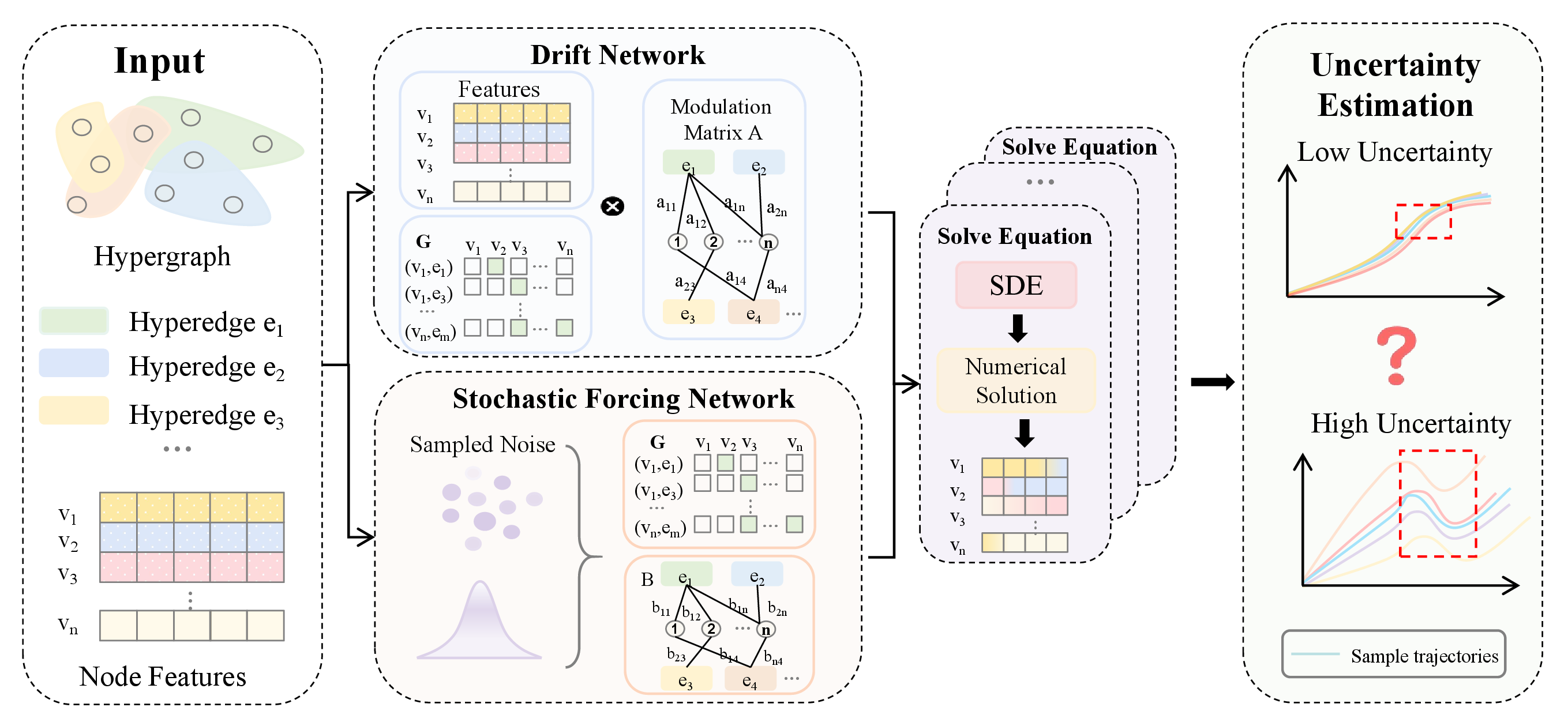
Combining the deterministic drift in Eq. 9 with the stochastic forcing in Eq. 13 , we obtain the proposed structure-informed HyperNSD: \[\mathrm d\mathbf{X}(t)=-\mathbf{G}^{\top}\mathbf{A}_\theta(\mathbf{X}(t))\mathbf{G}\mathbf{X}(t)\mathrm dt+\mathbf{G}^{\top} \mathbf{B}_\phi(\mathbf{X}(t))\mathbf{G}\mathrm d\mathbf{W}(t), \label{eq:node95driven95hsde}\tag{14}\] with the initial condition \(\mathbf{X}(0)=\zeta(\mathbf{X}_{\text{init}})\in\mathbb{R}^{n\times d}\), where \(\zeta\) is a learnable input encoder. To simplify the notation and subsequent analysis, we denote the corresponding effective node-space diffusion operator by \(\boldsymbol{\Sigma}^{\phi}(\mathbf{X}(t))=\mathbf{G}^{\top}\mathbf{B}_{\phi}(\mathbf{X}(t))\mathbf{G}.\)

The drift term in Eq. 14 governs deterministic higher-order feature propagation, whereas the stochastic term injects adaptively modulated, structure-dependent stochastic perturbations through the same node–hyperedge incidence geometry. Therefore, both deterministic diffusion and stochastic representation variability are consistently defined over the hypergraph incidence domain.

4.2 Theoretical Analysis↩︎

By construction, the neural drift \(\mathbf{F}^{\theta}\) and diffusion coefficient \(\boldsymbol{\Sigma}^{\phi}\) combine the fixed hypergraph gradient operators with softmax-normalized, state-dependent modulation matrices. Consequently, they remain bounded in their modulation strengths and inherit local regularity from the neural compatibility functions. Their local Lipschitz continuity and linear-growth properties are formalized in the following proposition.

The proof is provided in Appendix 8.

We next establish the well-posedness and stability properties of Eq. 14 . Proposition 2 shows that the drift and diffusion coefficients satisfy the local regularity conditions required for local existence and uniqueness. To extend the local solution to a global one, we further exploit the dissipative structure of the drift term together with the uniform boundedness of the diffusion coefficient. These properties prevent finite-time explosion and yield explicit moment, energy, and stopped stability estimates, as summarized in the following theorem.

The proof of Theorem 1 is provided in Appendix 9.

Theorem 1 establishes that the proposed stochastic dynamics are globally well defined, energetically controlled, and locally stable with respect to perturbations of the initial state before the exit time. Beyond initial-state stability, we further examine how the HyperNSD solution changes when the underlying hypergraph structure is perturbed. The following theorem establishes a local mean-square stability result with respect to aligned perturbations of the hypergraph gradient operator.

The proof of Theorem 2 is provided in Appendix 10.

In addition to stability under structural perturbations, the factorization of both the drift and diffusion operators through the hypergraph gradient \(\mathbf{G}\) also imposes intrinsic geometric constraints on the stochastic dynamics. In particular, the null-space components are preserved, while stochastic variability is confined to the nontrivial structural modes induced by the hypergraph. These structure-constrained modes are characterized in the following theorem.

The proof of Theorem 3 is provided in Appendix 11.

Theorem 3 characterizes how the hypergraph gradient constrains both the conserved modes and the directions along which stochastic variability can propagate. A complementary requirement is that these structural properties should not depend on the arbitrary ordering of the nodes or incidence pairs. We therefore next establish the permutation equivariance of the HyperNSD dynamics under consistent relabeling of the hypergraph.

Let \(\pi\) be an arbitrary permutation of the node set, represented by a permutation matrix \(\Pi\in\mathbb{R}^{n\times n}\). The permutation \(\pi\) induces a permutation matrix \(\mathbf{S}\in\mathbb{R}^{N\times N}\) on the node–hyperedge incidence pairs, mapping \((e,v)\) to \((\pi(e),\pi(v))\). Let \(\mathcal{G}^{\pi}\) denote the relabeled hypergraph. Its hypergraph gradient matrix satisfies \[\mathbf{G}^{\pi}=\mathbf{S}\mathbf{G}\Pi^{\top}. \label{eq:permuted95gradient95operator}\tag{15}\]

Since the hyperedge aggregation operator is permutation invariant and the compatibility networks are shared across all incidence pairs, the deterministic and stochastic modulation matrices transform as \[\mathbf{A}_{\theta}^{\pi}(\Pi\mathbf{X})=\mathbf{S}\mathbf{A}_{\theta}(\mathbf{X})\mathbf{S}^{\top},\quad\mathbf{B}_{\phi}^{\pi}(\Pi\mathbf{X})=\mathbf{S}\mathbf{B}_{\phi}(\mathbf{X})\mathbf{S}^{\top}. \label{eq:permuted95modulation95matrices}\tag{16}\] As a result, \[\mathbf{F}_{\mathcal{G}^{\pi}}^{\theta}(\Pi\mathbf{X})=\Pi\mathbf{F}_{\mathcal{G}}^{\theta}(\mathbf{X}),\quad\boldsymbol{\Sigma}_{\mathcal{G}^{\pi}}^{\phi}(\Pi\mathbf{X})=\Pi\boldsymbol{\Sigma}_{\mathcal{G}}^{\phi}(\mathbf{X})\Pi^{\top}. \label{eq:permuted95HNSD95coefficients}\tag{17}\]

The proof is provided in Appendix 12.

Remark

The above theoretical results provide several implications for the proposed HyperNSD as a neural network architecture. First, the local Lipschitz and linear-growth properties of the neural drift and diffusion coefficients ensure that the continuous-depth stochastic representation dynamics are well defined, rather than being merely a formal SDE construction. Second, the moment and energy estimates show that the stochastic feature evolution remains controlled over finite diffusion horizons, which is important for stable forward propagation and numerical training. Third, the stopped stability estimates with respect to initial-state and hypergraph structural perturbations indicate that small changes in input representations or incidence structures lead to controlled changes in stochastic trajectories before leaving a bounded region. This provides a theoretical explanation for the robustness of HyperNSD under feature and structural distribution shifts. Fourth, the structure-constrained mode analysis shows that the stochastic forcing does not introduce arbitrary perturbations in the node space; instead, stochastic variability is restricted to the nontrivial structural subspace determined by the hypergraph gradient operator. Finally, permutation equivariance guarantees that the HyperNSD outputs are independent of arbitrary node or incidence ordering, which is a basic requirement for hypergraph neural networks. Therefore, these results connect the stochastic diffusion formulation with standard desiderata in neural network learning, including stable representation propagation, structure-aware robustness, geometry-preserving stochasticity, and permutation-consistent prediction.

4.3 Discretization of HyperNSD↩︎

Although HyperNSD is formulated as a continuous-time SDE, its practical implementation is a finite-depth neural architecture. Specifically, each HyperNSD layer corresponds to one Euler–Maruyama step [41], and an \(L\)-layer HyperNSD performs \(L\) successive numerical updates over the diffusion horizon \([0,T]\).

We discretize the diffusion interval \([0,T]\) into \(L\) uniform subintervals, \[0=t_0<t_1<\cdots<t_L=T,\quad t_k=kh,\quad h=\frac{T}{L},\] where \(L\) denotes the number of HyperNSD layers and \(h\) is the step size associated with each layer. The Wiener increment corresponding to the \(k\)-th layer is defined as \[\Delta\mathbf{W}_k=\mathbf{W}(t_{k+1})-\mathbf{W}(t_k)\in\mathbb{R}^{n\times d}. \label{eq:wiener95increment}\tag{18}\]

Since the feature dimensions of \(\mathbf{W}(t)\) are mutually independent, the columns of \(\Delta\mathbf{W}_k\) are independent Gaussian random vectors satisfying \[\Delta\mathbf{W}_{k,j}\sim\mathcal{N}\left(0,h\mathbf{I}_n\right),\qquad j=1,\ldots,d,\] where \(\mathbf{I}_n\) denotes the identity matrix.

Let \(\mathbf{X}^{(k)}\) denote the node representation after the \(k\)-th HyperNSD layer, with \(\mathbf{X}^{(0)}=\mathbf{X}(0).\) Applying the Euler–Maruyama method to Eq. 14 gives the layer-wise update \[\begin{align} \mathbf{X}^{(k+1)}=\mathbf{X}^{(k)} &-h\mathbf{G}^{\top}\mathbf{A}_{\theta}\left(\mathbf{X}^{(k)}\right)\mathbf{G}\mathbf{X}^{(k)}\\ &+\mathbf{G}^{\top}\mathbf{B}_{\phi}\left(\mathbf{X}^{(k)}\right)\mathbf{G}\Delta\mathbf{W}_k, \end{align} \label{eq:layerwise95euler95HNSD}\tag{19}\] for \(k=0,\ldots,L-1\). Therefore, each HyperNSD layer consists of a deterministic diffusion residual and a stochastic structure-informed residual. For a fixed diffusion horizon \(T\), increasing the number of layers \(L\) decreases the step size \(h\) and produces a finer approximation of the continuous HyperNSD dynamics.

For the convergence analysis, let \(\mathbf{X}_k^h=\mathbf{X}^{(k)}\) and define the continuous-time Euler–Maruyama interpolation \[\begin{align} \overline{\mathbf{X}}^{h}(t)={} &\mathbf{X}(0)+\int_0^t\mathbf{F}^{\theta}\left(\mathbf{X}_{\nu_s^h}^h\right) \mathrm ds+\int_0^t\boldsymbol{\Sigma}^{\phi}\left(\mathbf{X}_{\nu_s^h}^h \right)\mathrm d\mathbf{W}(s), \end{align} \label{eq:continuous95em95interpolation}\tag{20}\] where \(\nu^h_s=\max\{k:t_k\leq s\}.\) At each grid point, we have \(\overline{\mathbf{X}}^{h}(t_k)=\mathbf{X}_k^h=\mathbf{X}^{(k)}.\)

The proof is provided in Appendix 13.

4.4 Loss Function, Uncertainty Estimation, and Complexity↩︎

4.4.1 Training Objective↩︎

Let \(\Theta\) denote all trainable parameters of HyperNSD. We adopt the distributional uncertainty loss [42] \[\mathcal{L}=\mathbb{E}_{\hat{\mathbb{P}}(X(T))} \left[\mathcal{H}[\mathbb{P}(y^{*}|\mathbf{X},\mathcal{G}),\mathbb{P}(y| \mathbf{X}(T))]\right], \label{eq:expected95pathwise95loss}\tag{21}\] where \(\hat{\mathbb{P}}(\mathbf{X}(T))=\hat{\mathbb{P}}(\mathbf{X}(T)|\mathbf{X}(0),\Theta,\mathcal{G})\) denotes the conditional distribution of the terminal node representations induced by the stochastic diffusion dynamics. \(\mathbb{P}(y^{*}|\mathbf{X},\mathcal{G})\) denotes the true class distribution and \(\mathbb{P}(y|\mathbf{X}(T))\) is the conditional predictive distribution produced by the output decoder \(\xi\). Rather than optimizing the cross-entropy associated with a single deterministic representation, the proposed objective minimizes the expected path-conditioned cross-entropy over the distribution of stochastic terminal representations. It therefore accounts for predictive variability induced by the stochastic representation dynamics during training.

4.4.2 Uncertainty Estimation↩︎

After training, HyperNSD generates \(M\) stochastic samples from \(\hat{\mathbb{P}}(\mathbf{X}(T))\) to estimate both aleatoric and epistemic uncertainties. Each sample corresponds to an independent numerical realization of the proposed hypergraph stochastic diffusion equation and produces a distinct terminal node representation \(\mathbf{X}(T)\). In this framework, the aleatoric component is estimated by \(\mathbb{E}_{\hat{\mathbb{P}}(X(T))} \left[\mathcal{H}[\mathbb{P}(y| \mathbf{X}(T))]\right]\), while the trajectory-induced epistemic component can be calculated by the variance of the final solution \(\mathbf{X}(T)\). To obtain structure-aware uncertainty estimates, HyperNSD jointly incorporates node attributes and node–hyperedge incidence information into the deterministic drift and stochastic forcing networks. The stochastic forcing term maps node-space Wiener perturbations to the incidence domain, adaptively modulates them according to local node–hyperedge contexts, and propagates them back to the node space, thereby capturing both representation variability and higher-order structural dependencies. This sampling-and-estimation procedure follows the standard SDE-based uncertainty estimation paradigm [13], [43] and resembles ensemble inference; however, HyperNSD requires only a single trained model, reducing training and storage costs while generating multiple stochastic predictions through repeated forward trajectories. A detailed explanation of how predictive uncertainty is computed and used for the detection tasks is provided in Appendix 14.

4.4.3 Complexity Analysis↩︎

Let \(n\) denote the number of nodes, \(N=|\mathcal{I}|\) the number of node–hyperedge incidence pairs, and \(d\) the feature dimension.

Under fixed-width drift and diffusion coefficient networks, computing \(\mathbf{F}^{\theta}\) and \(\boldsymbol{\Sigma}^{\phi}\) requires \(\mathcal{O}(Nd)\) operations. Sampling the Gaussian increment \(\Delta\mathbf{W}\) requires \(\mathcal{O}(nd)\) operations. The per-layer complexity of one stochastic trajectory is therefore \(\mathcal{O}(Nd).\) A complete stochastic trajectory contains \(L\) Euler–Maruyama layers. Hence, the computational complexity of one forward trajectory is \(\mathcal{O}(LNd).\) HyperNSD generates \(M\) independent stochastic trajectories. Consequently, the total forward-pass complexity is \(\mathcal{O}(MLNd),\) excluding the task-specific readout and decoder. The empirical runtime comparison is given in Appendix 15.

5 Experiments↩︎

This section evaluates HyperNSD on six hypergraph benchmarks under label leave-out, feature interpolation, and structure manipulation settings. We compare HyperNSD with representative uncertainty estimation and hypergraph learning methods using out-of-distribution (OOD) detection and misclassification detection. We further conduct ablation studies, graph-expansion comparisons, and uncertainty visualizations to examine the effectiveness of the incidence-aware stochastic diffusion mechanism. The source code will be available at https://github.com/CASZhouzhiheng/HyperNSD.

3pt

5.1 Experimental Setup↩︎

5.1.0.1 Datasets

We evaluate our model on six benchmark hypergraph datasets including four citation datasets (Cora, Cora-CA, CiteSeer and DBLP) [20], [44] and two real–world datasets (ModelNet40, NTU2012) [45], [46]. For each dataset, we randomly divide the samples into training, validation, and test sets using a 50%/25%/25% split. All experiments are independently repeated ten times with different random seeds, and we report the average performance over the ten runs. Detailed statistics of the evaluated datasets are summarized in Table ¿tbl:tab:dataset95stats?. We provide detailed dataset information in Appendix 16.2.

5.1.0.2 OOD Shift Construction

We synthetically generate OOD samples using three types of distribution shifts.

• Label leave-out. We construct semantic shifts by retaining a subset of classes as in-distribution data and treating the remaining classes as OOD samples. Specifically, samples with class labels greater than 3 are treated as OOD for Cora, Cora-CA, and DBLP; samples with class labels greater than 2 are treated as OOD for Citeseer; samples with class labels greater than 20 are treated as OOD for ModelNet40; and samples with class labels greater than 33 are treated as OOD for NTU2012. All remaining samples are used as ID data.

• Feature interpolation. We construct attribute-level OOD samples by randomly interpolating the node features of selected target samples with features drawn from other nodes. The original hypergraph data are retained as ID data, whereas the interpolated hypergraph data are regarded as OOD data. The hypergraph incidence structure remains unchanged.

• Structure manipulation. We generate structural OOD samples through degree-preserving incidence rewiring. Specifically, two existing incidences satisfying \[H_{u,e_1}=1,\quad H_{v,e_2}=1, andH_{u,e_2}=0,\quad H_{v,e_1}=0\] are randomly selected. We then replace \((u,e_1)\) and \((v,e_2)\) with \((u,e_2)\) and \((v,e_1)\), respectively. This operation preserves the degrees of nodes \(u\) and \(v\), as well as the cardinalities of hyperedges \(e_1\) and \(e_2\), while altering the local node–hyperedge associations. The rewiring ratio \(\gamma\) is set to 0.5 in all experiments. The original hypergraph data are retained as ID data, whereas the incidence rewiring hypergraph data are regarded as OOD data. The hypergraph node features remain unchanged.

width=

5.1.0.3 Implementation Details

For HyperNSD, the diffusion horizon is fixed to \(T=1\), while the remaining key hyperparameters are selected by grid search according to validation performance. Specifically, the hidden layer dimension is chosen from \(\{16,32,64,128,256\}\), the learning rate from \(\{10^{-4},10^{-3},10^{-2}\}\), the number of training sample trajectories \(M\) from \(\{1,3,5,7\}\), and the Euler–Maruyama step size \(h\) from \(\{0.01,0.05,0.1,0.2\}\). All models are trained for 200 epochs. To ensure a fair comparison, HyperNSD and all competing methods use the same hidden layer dimension under each experimental setting. The baseline methods are implemented and fully optimized following their recommended configurations, and training is continued until stable convergence is achieved.

5.1.0.4 Baselines

We compare HyperNSD with three categories of representative methods. The first category consists of conventional OOD detection approaches, including MSP [32], ODIN [33], and Mahalanobis [34]. Since these methods were originally developed for Euclidean or graph data, we replace their original feature encoders with a common hypergraph convolutional encoder to ensure compatibility with hypergraph-structured inputs. The second category includes graph uncertainty estimation methods, namely GNNSafe [12], GPN [17], GNSD [13], and LGNSDE [18]. The third category comprises hypergraph neural network methods, including HGNN [5], HyperGCN [20], ensemble–based HyperGCN (HGCN-Ens) [11], HNDiffN [30], HND [8], and HyperGOOD [47].

For the GNN-based baselines, each hypergraph dataset is first converted into a pairwise graph using clique expansion, after which the corresponding graph models are trained and evaluated. For deterministic GNN and HGNN baselines, aleatoric uncertainty is used for all detection tasks. For uncertainty-aware methods, epistemic uncertainty is adopted for OOD detection, whereas aleatoric uncertainty is used for misclassification detection, following prior studies [17], [39]. Details of all baselines are provided in Appendix 16.3.

5.1.0.5 Evaluation Metrics

An effective uncertainty-aware HGNN should accurately identify anomalous samples while maintaining strong predictive performance on in-distribution data. Accordingly, we adopt AUROC, AUPR, FPR95, and in-distribution classification accuracy (ID ACC) as the evaluation metrics. Higher AUROC, AUPR, and ID ACC indicate better performance, whereas lower FPR95 is preferred. In each comparison, the best result is highlighted in bold and the second-best result is underlined. Further details of these metrics are provided in Appendix 16.4.

width=

5.2 OOD Detection↩︎

We evaluate our model in three OOD scenarios (label leave-out, feature interpolation, and structure manipulation denote by L, F, and S, respectively). The OOD detection results are provided in Table ¿tbl:table:ood95result? and more experimental results are provided in Appendix 16.5 (Tables ¿tbl:table:ood95cora?–¿tbl:table:ood95std?). From Table ¿tbl:table:ood95result?, we draw the following observations. First, HyperNSD achieves the best AUROC in 16 out of 18 evaluation settings, including all feature interpolation and structure manipulation experiments. Compared with the strongest competing method in each setting, HyperNSD obtains its largest improvement of 4.18% on Cora-CA under feature interpolation. Moreover, it improves the average AUROC by 2.77% and 3.18% under feature interpolation and structure manipulation, respectively. Second, the consistent improvements across citation and real-world hypergraphs demonstrate that HyperNSD can provide more informative uncertainty scores for identifying OOD samples arising from semantic, attribute, and structural distribution shifts. Third, the particularly strong performance under structure manipulation indicates that directly modeling stochastic dynamics over the original node–hyperedge incidence domain is more effective than applying graph uncertainty methods to pairwise approximations of hypergraphs.

5.3 Misclassification Detection↩︎

Besides OOD detection, we also evaluate the ability of different methods to identify misclassified samples. Misclassification detection examines whether the estimated uncertainty can effectively distinguish incorrect predictions from correct ones at test time [32]. As shown in Table ¿tbl:table:mis?, HyperNSD achieves the best performance in 18 out of 24 evaluation settings across the six datasets. On average, compared with the strongest competing baseline for each metric, HyperNSD improves AUROC by 2.10%, AUPR succ by 1.49%, and AUPR err by 6.01%, while reducing FPR95 by 4.97%. These results demonstrate that the path-conditioned predictive entropy estimated by HyperNSD is highly informative for identifying incorrect predictions while preserving strong classification performance.

5.4 Comparison with Graph Expansions↩︎

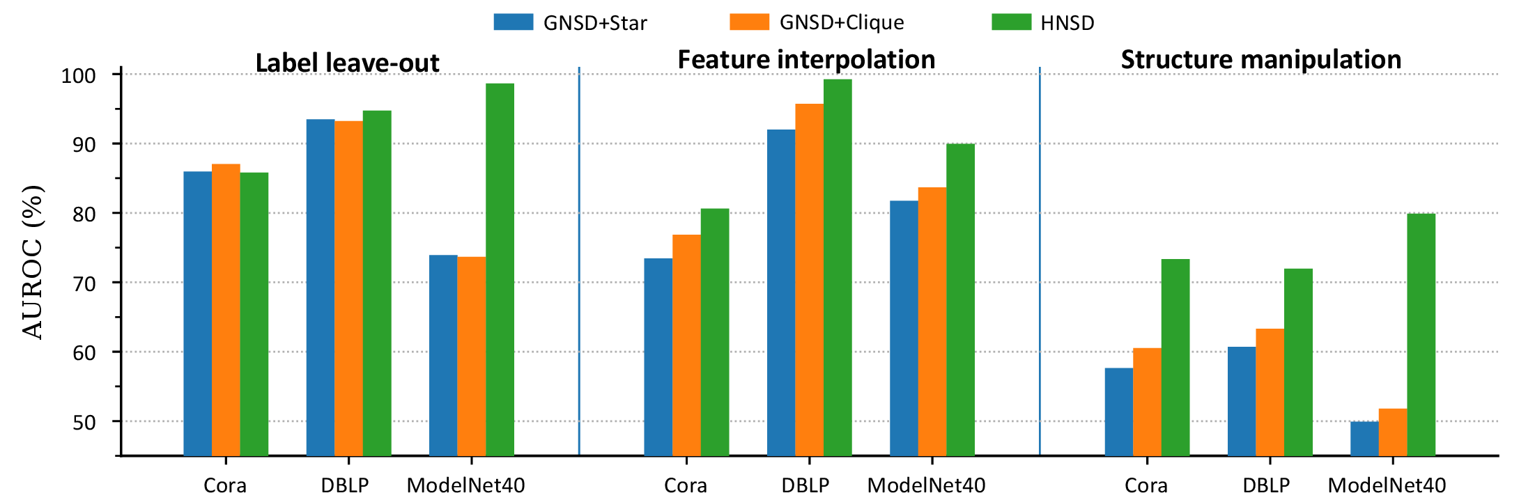
To examine the necessity of modeling stochastic diffusion directly over the original hypergraph incidence domain, we compare HyperNSD with GNSD implemented using star and clique expansions. As shown in Fig. 2, HyperNSD consistently achieves superior or competitive performance across the three OOD settings. Its advantage is especially pronounced under feature interpolation and structure manipulation, while remaining competitive under label leave-out. These results indicate that preserving the original node–hyperedge incidence geometry enables more effective uncertainty propagation and improves the detection of attribute- and structure-induced distribution shifts compared with pairwise graph expansions.

5.5 Model Variants↩︎

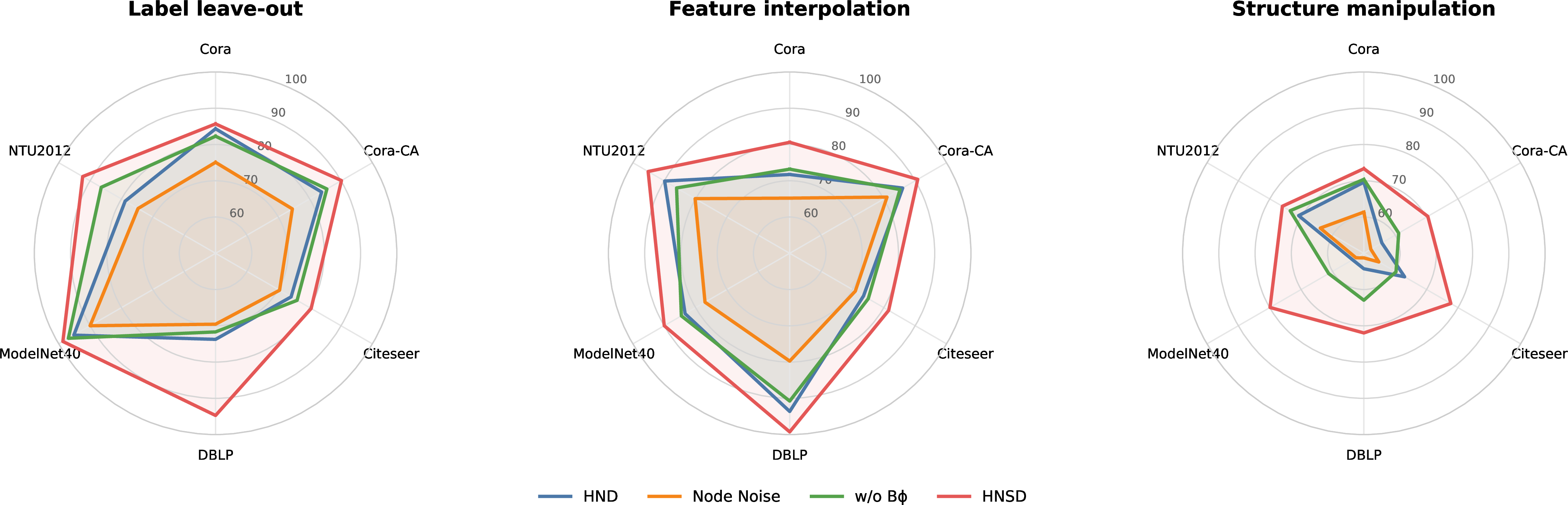
To investigate the effect of different noise modeling strategies, we compare HyperNSD with deterministic HND, a variant using node-level noise, and a variant without the learnable \(B_{\phi}\). As shown in Fig. 3, the complete HyperNSD consistently outperforms its variants across the three OOD settings. The deterministic HND and the variant with simple node-level noise generally achieve lower performance, indicating that stochasticity alone is insufficient for reliable OOD detection. Removing \(B_{\phi}\) also leads to performance degradation, particularly under feature and structure shifts. These results confirm that incidence-aware stochastic forcing and adaptive noise modulation are both important to the effectiveness of HyperNSD.

5.6 Perturbation Intensity Analysis↩︎

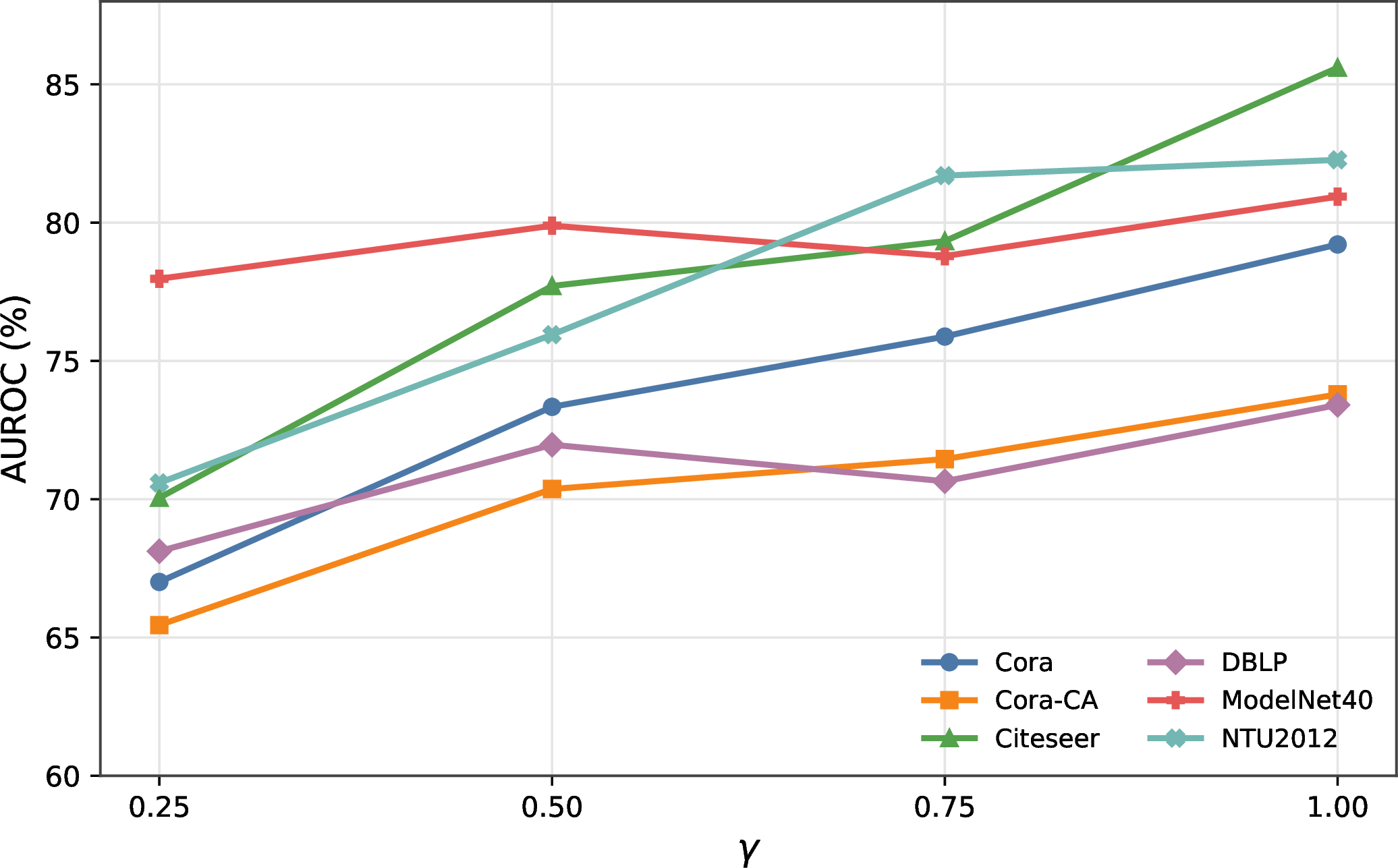
We further investigate the influence of the rewiring ratio \(\gamma\) on the OOD detection performance of HyperNSD, with the results reported in Fig. 4. From Fig. 4, we draw the following observations. First, the AUROC generally increases as the rewiring ratio grows across most datasets, indicating that stronger structural shifts produce more distinguishable stochastic representations between ID and OOD samples. Second, HyperNSD still maintains satisfactory detection performance under relatively mild structural perturbations, demonstrating its ability to capture subtle structural distribution shifts. Third, although slight fluctuations are observed on several datasets, the overall performance remains stable or improves with increasing rewiring ratio. These results demonstrate that the uncertainty estimated by HyperNSD responds effectively and consistently to different levels of hypergraph structural perturbations.

5.7 Visual Analysis↩︎

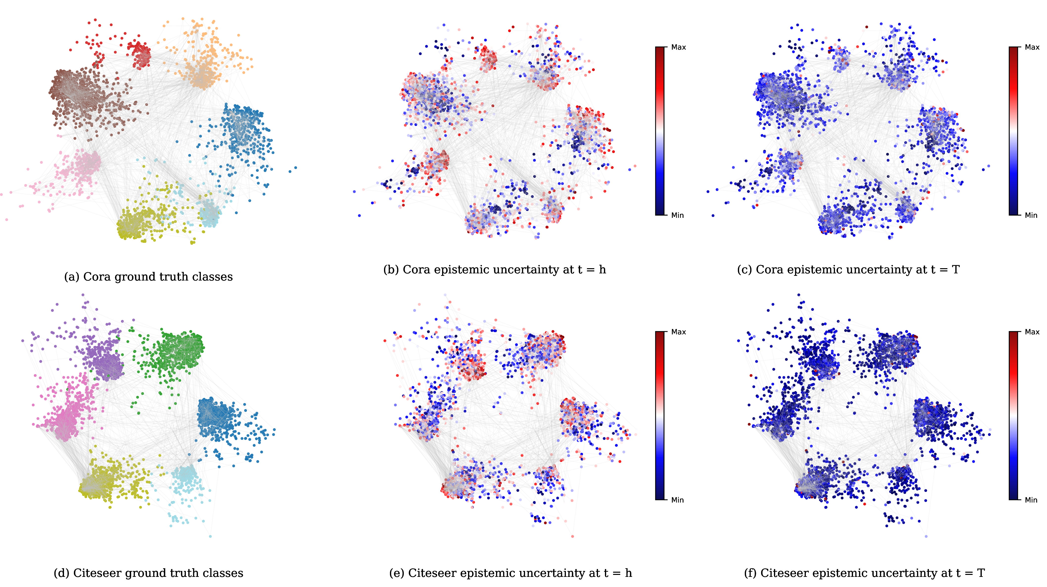
To qualitatively examine how uncertainty evolves during stochastic diffusion, we visualize the node-level epistemic uncertainty at the \(t=h\) and terminal states on Cora and Citeseer. As shown in Fig. 5, the \(t=h\) representations exhibit broadly distributed high-uncertainty regions, whereas the uncertainty is substantially reduced after diffusion. Most nodes within coherent class clusters become more certain, while relatively high uncertainty remains around class boundaries and structurally ambiguous regions. These observations indicate that HyperNSD progressively refines node representations while preserving uncertainty for difficult or potentially unreliable samples.

6 Conclusion↩︎

In this paper, we presented Hypergraph Neural Stochastic Diffusion (HyperNSD), an SDE-based framework for uncertainty estimation on hypergraphs. HyperNSD models node representations as stochastic processes evolving over the node–hyperedge incidence domain, where a learnable drift term governs deterministic higher-order feature propagation and an incidence-aware stochastic forcing term captures structure-dependent representation variability. We established theoretical guarantees for the proposed dynamics, including global well-posedness, finite-horizon moment control, stability under initial-state and structural perturbations, structure-constrained stochastic modes, permutation equivariance, and convergence of the Euler–Maruyama discretization. Extensive experiments on six hypergraph benchmarks demonstrated that HyperNSD provides informative uncertainty estimates for OOD and misclassification detection while maintaining competitive in-distribution predictive performance. Additional comparisons and analyses further verified the advantages of directly modeling stochastic diffusion over the original incidence structure and the effectiveness of adaptively modulated incidence-level stochastic perturbations. Overall, HyperNSD provides a principled stochastic-dynamical foundation for uncertainty-aware higher-order representation learning. Future work will investigate more expressive stochastic processes and extend the framework to dynamic, heterogeneous, and large-scale hypergraphs.

7 Proof of Proposition 1↩︎

We first recall the definition of a \(\mathcal{Q}\)-Wiener process in a separable Hilbert space [40].

Based on Definition 1, we now verify that the incidence-space process \(\mathbf{Z}(t)=\mathbf{G}\mathbf{W}(t)\) constructed in the proposed HSDE in Eq. 8 is a \(\mathcal{Q}\)-Wiener process.

8 Proof of Proposition 2↩︎

9 Proof of Theorem 1↩︎

10 Proof of Theorem 2↩︎

Consider two hypergraphs \(\mathcal{G}\) and \(\mathcal{G}'\) defined on the same node set. After consistently aligning their incidence coordinates, let their hypergraph gradient matrices be \(\mathbf{G},\mathbf{G}' \in\mathbb{R}^{N\times n}.\)

The two HyperNSD systems share the same trainable parameters and are driven by the same node-space Wiener process \(\mathbf{W}(t)\): \[\label{twosystem} \begin{align} d\mathbf{X}^{\mathbf{G}}(t) &= \mathbf{F}^{\theta,\mathbf{G}} \bigl(\mathbf{X}^{\mathbf{G}}(t)\bigr)dt + \mathbf{\Sigma}^{\phi,\mathbf{G}} \bigl(\mathbf{X}^{\mathbf{G}}(t)\bigr)d\mathbf{W}(t),\\ d\mathbf{X}^{\mathbf{G}'}(t) &= \mathbf{F}^{\theta,\mathbf{G}'} \bigl(\mathbf{X}^{\mathbf{G}'}(t)\bigr)dt + \mathbf{\Sigma}^{\phi,\mathbf{G}'} \bigl(\mathbf{X}^{\mathbf{G}'}(t)\bigr)d\mathbf{W}(t), \end{align}\tag{48}\]

where \[\begin{align} \mathbf{F}^{\theta,\mathbf{G}}(\mathbf{X}) &=-\mathbf{G}^{\top}\mathbf{A}_{\theta}^{\mathbf{G}}(\mathbf{X}) \mathbf{G}\mathbf{X},\\ \mathbf{\Sigma}^{\phi,\mathbf{G}}(\mathbf{X}) &= \mathbf{G}^{\top}\mathbf{B}_{\phi}^{\mathbf{G}}(\mathbf{X}) \mathbf{G}. \end{align}\]

The notation \(\mathbf{A}_{\theta}^\mathbf{G}\) and \(\mathbf{B}_{\phi}^\mathbf{G}\) emphasizes that the incidence-wise modulation coefficients depend on the hypergraph structure through the node–hyperedge aggregation contexts. We first prove the following lemma.

11 Proof of Theorem 3↩︎

12 Proof of Proposition 3↩︎

13 Proof of Proposition 4↩︎

14 Using uncertainty for Detection↩︎

Our experiments consider two uncertainty-aware tasks: OOD detection and misclassification detection. Taking OOD detection as an example, we construct OOD samples through label leave-out, feature interpolation, or structure manipulation, as described in Section 5. HyperNSD then generates multiple stochastic representation trajectories for each ID and OOD node, and quantifies node-level uncertainty from the variability of their terminal representations. Since the model is trained on ID data, ID representations are generally more stable and exhibit lower uncertainty, whereas OOD nodes contain unseen semantic, attribute, or structural patterns and therefore tend to produce greater trajectory variability. The resulting uncertainty scores are used to distinguish ID from OOD nodes. Misclassification detection follows an analogous uncertainty-ranking principle, using aleatoric uncertainty as the detection score.

Because the pathwise OOD score is estimated directly in the node-representation space, it is not intrinsically tied to a classification decoder and can, in principle, be adapted to regression and representation-based anomaly detection. In contrast, many deterministic confidence-based methods rely on classification logits or probabilities and require task-specific modifications for non-classification settings. This representation-level formulation therefore improves the flexibility and general applicability of HyperNSD.

15 Runtime Comparison↩︎

We provide an empirical comparison of the per-epoch training time between HyperNSD and nine representative baselines under the label leave-out setting on Cora. As shown in Fig. 6, deterministic hypergraph models such as HGNN, HyperGCN, HND, and HNDiffN require relatively low computational cost, whereas stochastic diffusion methods introduce additional overhead due to numerical integration and stochastic trajectory generation. HyperNSD requires 0.76 seconds per epoch, which is higher than GNSD and LGNSDE because it performs both deterministic and stochastic propagation directly over the node–hyperedge incidence domain. Nevertheless, its runtime remains below that of HGNN-Ensemble and stays within one second per epoch. These results demonstrate that HyperNSD achieves reliable uncertainty estimation and higher-order stochastic modeling with an acceptable computational cost.

16 Experimental Details↩︎

16.1 Experimental Environment↩︎

All experiments were conducted on a Linux server running Ubuntu 22.04, equipped with an Intel(R) Xeon(R) E5-2699 v4 CPU at 2.20 GHz, 384 GB of RAM, and an NVIDIA GeForce RTX 3090 GPU with 24 GB of memory. HyperNSD and all baseline methods were implemented in Python 3.10 using PyTorch 2.6.0.

16.2 Dataset Information↩︎

The datasets used in our experiments are all publicly available as common benchmarks for evaluating hypergraph learning models.

• Cora [20], [44] is a co-citation hypergraph constructed from a scientific publication network. Each node represents a paper, while each hyperedge connects the papers cited by the same publication. The task is to predict the research topic of each paper. The dataset contains 2708 nodes, 1579 hyperedges, 1433-dimensional bag-of-words features, and 7 classes.

• Cora-CA [20] is a co-authorship hypergraph constructed from the Cora publication corpus. Each node denotes a paper, and each author defines a hyperedge connecting all papers written by that author. The prediction task is to classify each paper into its corresponding research topic. The dataset contains 2708 nodes, 1072 hyperedges, 1433 features, and 7 classes.

• Citeseer [20], [44] is a co-citation hypergraph of scientific publications. Each node corresponds to a paper, and each hyperedge groups the papers cited by the same publication. Node attributes are represented by bag-of-words features, and the task is to predict the topic of each paper. The dataset contains 3312 nodes, 1079 hyperedges, 3703 features, and 6 classes.

• DBLP [20] is a co-authorship hypergraph constructed from computer science publications. Each node represents a paper, while each author forms a hyperedge connecting all papers authored by that individual. The task is to classify papers into different research areas. The dataset contains 41302 nodes, 22363 hyperedges, 1425 features, and 6 classes.

• ModelNet40 [45] is a large-scale 3D object dataset containing CAD models from 40 object categories. Each 3D object is treated as a node, and hyperedges are constructed by connecting each object with its 10 nearest neighbors in the visual feature space. The dataset contains 12311 nodes, 24622 hyperedges.

• NTU2012 [46] is a 3D shape dataset containing objects from 67 semantic categories. Each object is represented as a node, and hyperedges are generated by grouping each object with its 10 nearest neighbors according to visual-feature similarity. The dataset contains 2012 nodes, 4024 hyperedges.

16.3 Baseline Descriptions↩︎

• MSP [32] uses the maximum probability produced by the softmax classifier as the confidence score. It is based on the observation that correctly classified ID samples generally receive higher maximum softmax probabilities than misclassified or OOD samples.

• ODIN [33] improves softmax-based OOD detection through temperature scaling and small input perturbations. These operations enlarge the separation between the confidence-score distributions of ID and OOD samples without modifying the pretrained classifier.

• Mahalanobis [34] models the intermediate representations of each class using class-conditional Gaussian distributions. The Mahalanobis distance between a test representation and its closest class distribution is then used to derive the OOD confidence score.

• GNNSafe [12] is an energy-based OOD detection method designed for graph-structured data. It extracts node-level energy scores from a GNN trained with the standard classification objective and further propagates these scores over the graph to exploit relational dependencies. Since auxiliary OOD samples are unavailable in our setting, we adopt its variant without OOD exposure.

• GPN [17] extends posterior networks to graph-structured data and represents node predictions using Dirichlet distributions. It estimates class-specific pseudo-counts through density estimation and propagates the resulting evidence across neighboring nodes to quantify predictive uncertainty.

• GNSD [13] formulates graph representation learning as a stochastic diffusion process driven by a structure-dependent Wiener process. It estimates predictive uncertainty from multiple stochastic representation trajectories, thereby modeling how uncertainty evolves and propagates over pairwise graph structures.

• LGNSDE [18] extends graph neural ordinary differential equations to latent graph neural stochastic differential equations. By introducing Brownian perturbations into the continuous latent dynamics, it generates stochastic node representations and quantifies uncertainty from their predictive variability.

• HGNN [5] introduces a spectral hypergraph convolution operator based on the normalized hypergraph Laplacian. It propagates information through node–hyperedge–node interactions and captures higher-order dependencies encoded by the incidence structure.

• HyperGCN [20] approximates each hyperedge using a set of representative pairwise connections and subsequently applies GCN-style propagation to the resulting graph. This construction enables conventional graph convolution to process hypergraph-structured data.

• HGCN-Ens [11] trains 10 independently initialized HyperGCN models and aggregates their predictive distributions. The disagreement among the ensemble members is used to estimate predictive uncertainty, at the cost of repeated training and increased model storage.

• HNDiffN [30] interprets hypergraph representation learning from a diffusion perspective and derives neural propagation layers from hypergraph diffusion dynamics. It provides a deterministic diffusion-based baseline for modeling higher-order feature propagation.

• HND [8] formulates hypergraph message passing as a nonlinear anisotropic diffusion process defined through hypergraph gradient and divergence operators. Learnable incidence-level coefficients adaptively regulate deterministic feature transport between nodes and hyperedges.

• HyperGOOD [47] is an energy-based framework specifically developed for OOD detection on hypergraphs. It combines multi-scale spectral decomposition with structure-aware uncertainty propagation to identify samples whose higher-order relational contexts differ from those observed during training.

16.4 Evaluation Metrics↩︎

Following prior studies [12], [17], [43], we evaluate both detection reliability and in-distribution predictive performance using AUROC, AUPR, FPR95, and ID ACC.

• AUROC denotes the area under the receiver operating characteristic curve. It evaluates the ability of a model to distinguish in-distribution and out-of-distribution samples across all possible decision thresholds. A higher AUROC indicates stronger discrimination performance.

• AUPR is the area under the precision–recall curve. It is particularly informative when the numbers of positive and negative samples are imbalanced, and is therefore widely adopted for OOD detection. For misclassification detection, we report both AUPR succ, where correctly classified samples are treated as positive, and AUPR err, where incorrectly classified samples are treated as positive.

• FPR95 measures the false positive rate when the true positive rate is fixed at 95%. It reflects the extent to which negative samples are incorrectly identified as positive under a high-recall operating point. Lower FPR95 indicates better detection performance.

• ID ACC denotes the classification accuracy evaluated on in-distribution test samples. It is used to assess whether a method can provide reliable uncertainty estimates without sacrificing its predictive performance on normal data.

16.5 More Empirical Results↩︎

In Tables ¿tbl:table:ood95cora?–¿tbl:table:ood95ntu2012?, we report the AUROC/AUPR/FPR95 and in-distribution test accuracy on all datasets as complementary results to Table ¿tbl:table:ood95result? in the main text. In addition, Table ¿tbl:table:ood95std? reports the standard deviations of AUROC scores for OOD detection over ten independent runs, and Table ¿tbl:table:mis95std? reports the standard deviations of misclassification detection metrics.

width=

width=

width=

width=

width=

width=

width=

width=

References↩︎

---

1. This work was supported by the National Natural Science Foundation of China (No.12231018 and No.12471330), the Shandong Provincial Natural Science Foundation (No.ZR2025MS71) and the Postdoctoral Innovation Program of Shandong Province (No.SDCX-ZG-202603012). (Corresponding author: Xingqin Qi, Guiying Yan.)↩︎

2. Zhiheng Zhou, Dengyi Zhao and Xingqin Qi are with the School of Mathematics and Statistics, Shandong University, Weihai, Shandong 264209, China (e-mail: zhouzhiheng@amss.ac.cn; zhaodengyi@mail.sdu.edu.cn; qixingqin@sdu.edu.cn).↩︎

3. Mengyao Zhou and Guiying Yan are with the Academy of Mathematics and Systems Science, Chinese Academy of Sciences and also with the University of Chinese Academy of Sciences, Beijing 100190, China (e-mail: zhoumengyao@amss.ac.cn; yangy@amss.ac.cn).↩︎