Naming the Concepts Classifiers Rely On: Language-Anchored Decomposition for Faithful Explanation
July 08, 2026
Abstract
Deep neural networks are widely deployed in high-stakes visual applications where interpretability is critical, yet existing explanations face a trade-off: post-hoc concept methods recover factors that are faithful to a model’s behavior but unnamed, while naming and by-design methods attach human-readable concepts only by retraining or altering the classifier. We propose Language-Anchored Decomposition (LAD), a post-hoc framework that delivers concepts which are simultaneously named, faithful, and obtained without modifying the model. For each class, a large language model proposes a concept vocabulary that CLIP-based similarity maps localize across image regions. Inverting standard non-negative matrix factorization, LAD fixes these language-grounded maps as the coefficient matrix and learns only a concept basis that reconstructs the frozen encoder’s activations, so naming becomes a structural constraint and the model’s own feature geometry determines which concepts are retained. Removing this anchor preserves accuracy but collapses attribution faithfulness. Across natural-image, scene, and medical-imaging benchmarks, LAD produces spatially precise explanations that are decision-relevant under both concept insertion and deletion, while uniquely providing stable, human-interpretable concept names. Code is available at: https://github.com/machine-intelligence-lab-wvu/LAD.
1 Introduction↩︎
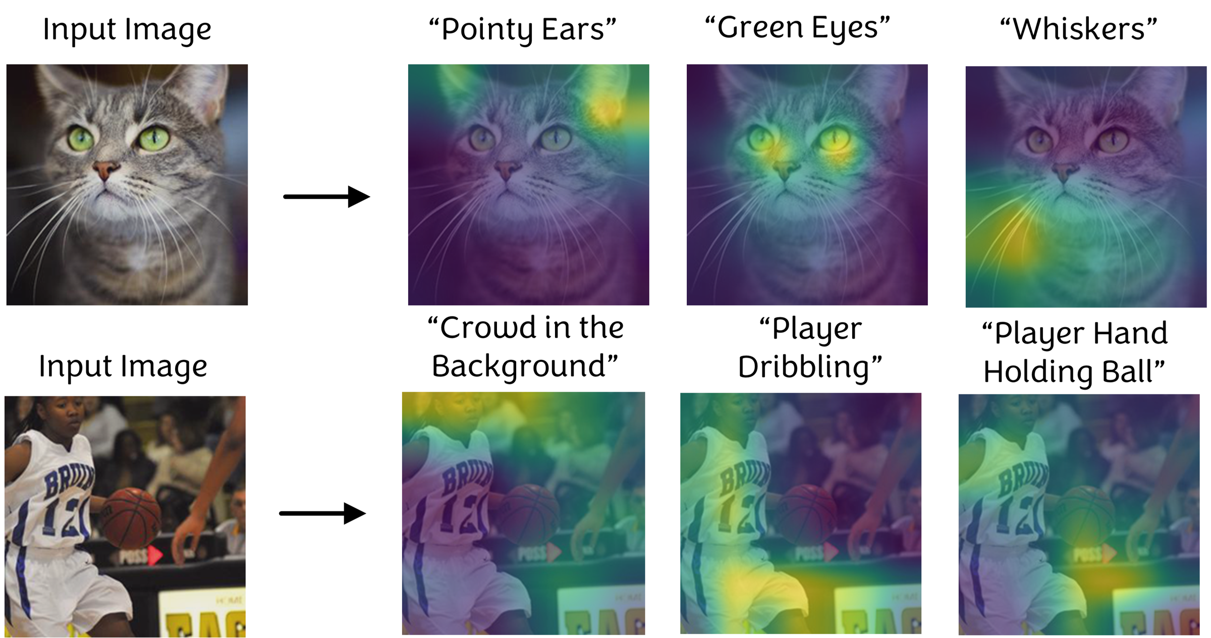
Interpreting the decision mechanisms of deep visual models is crucial for diagnosing failures, mitigating biases, and ensuring responsible deployment in high-stakes applications. Post-hoc attribution methods such as Grad-CAM [1] and Integrated Gradients [2] visualize the input regions most influential to a prediction, but they operate at the pixel level and emphasize low-level activations rather than the high-level cues humans reason with, offering limited semantic insight into a model’s decision process [3]. Concept-based explanations address this by attributing predictions to human-interpretable units such as object parts and visual attributes [4]–[6].
Existing concept-based methods, however, fall into two families that each pay a price. The first is post-hoc concept discovery. Building on TCAV [4], unsupervised methods such as ACE [6], ICE [7], and CRAFT [5] extract concepts via clustering or Non-Negative Matrix Factorization (NMF), and FACE [8] further aligns the decomposition with classifier logits to improve faithfulness. These methods are faithful to the model, but the recovered factors are unnamed: the same factor index can correspond to different visual elements across images, so a human must label each factor after the fact and consistency is not guaranteed. The second family attaches names directly. Concept Bottleneck Models [9], their label-free variants [10], and spatial extensions such as Show and Tell [11] predict named concepts before classification, while neuron-naming methods such as LaViSE [12] train an auxiliary explainer to describe individual filters. These methods produce names, but at a cost: by-design models replace the classifier head with a newly trained predictor, so the explained model is no longer the deployed one [13], and neuron-naming methods describe units without testing whether the named concepts are actually responsible for predictions. No prior method delivers concepts that are simultaneously named, faithful, and obtained without modifying the model.
We fill this gap with Language-Anchored Decomposition (LAD) by inverting the standard decomposition. For each target class, a large language model proposes a class-specific concept vocabulary; for “cat”, the proposals may include “pointy ears,” “green eyes,” and “whiskers.” We then use CLIP [14] image–text similarity to localize each concept across image regions. Rather than learning latent coefficients as in NMF, LAD fixes these language-grounded similarity maps as the coefficient matrix and learns only a concept basis that reconstructs the frozen encoder’s activations. Naming therefore becomes a structural constraint rather than a post-hoc label, and the model’s own feature geometry, not CLIP alone, determines which named concepts are retained. LAD needs no auxiliary training and no concept annotations, and tests faithfulness by reconstruction rather than describing units in isolation.
Crucially, the language anchor is not cosmetic. Replacing the fixed language-grounded coefficients with learned ones, which recovers standard unsupervised NMF on the same activations, preserves classification accuracy but sharply reduces attribution faithfulness. (5.5). The anchor changes which basis directions are discovered, steering them toward classifier-meaningful structure, and the reconstruction objective reshapes the initial CLIP similarities so that concepts inconsistent with the encoder’s evidence are suppressed, mitigating known biases in CLIP-style models. 1 illustrates the resulting explanations, which recover fine-grained part-level concepts (top) and higher-level scene structure (bottom), each localized and paired with a natural-language name.
Main Contributions:
A post-hoc concept discovery framework, Language-Anchored Decomposition (LAD), that inverts NMF by fixing language-grounded CLIP similarity maps as the coefficient matrix and learning only the concept basis against frozen encoder activations. Naming is enforced structurally, with no retraining and no manual concept annotations.
Evidence that the language anchor is functional rather than cosmetic: removing it preserves accuracy but collapses deletion faithfulness, showing that language supervision determines which concept directions are discovered.
Evaluation across natural-image, scene, and medical benchmarks showing that LAD’s named concepts are decision-relevant under concept insertion and deletion, at faithfulness comparable to the strongest prior method.
2 Related Work↩︎
Interpretability methods fall into two broad approaches: post-hoc methods that interpret a model after training, and ante-hoc explanation-by-design architectures that constrain the model during learning.
Feature attribution: Saliency maps [15], Grad-CAM [1], Integrated Gradients [2], and perturbation-based variants [16], [17] attribute importance to input pixels. These pixel-level maps lack semantic interpretability and can be visually plausible yet unfaithful to the model’s decision [3], [18].
Post-hoc concept discovery: TCAV [4] quantifies sensitivity to user-defined concepts but needs manual annotation, while ACE [6], ICE [7], and CRAFT [5] automate discovery via clustering or Non-negative Matrix Factorization (NMF). FACE [8] improves faithfulness with a KL regularizer aligning reconstructed and original predictions. These methods are faithful but their factors are unnamed: a factor index may map to different visual elements across images, so each must be labeled after the fact with no consistency guarantee.
Naming individual units: A parallel line attaches language to model internals at the level of individual neurons or filters: Network Dissection [19] via overlap with annotated concept masks, and MILAN [20] and CLIP-Dissect [21] via open-vocabulary descriptions of top-activating regions. LaViSE [12] maps masked filter activations to a semantic space to describe filters, including unseen concepts. These methods differ from ours on two axes. First, granularity: they name single units, whereas decomposition-based discovery, including LAD, recovers concepts as directions in activation space (combinations of units), the unit at which NMF-style methods operate. Second, faithfulness: they produce descriptive labels without testing whether a named concept is causally responsible for a prediction, and several [12], [19], [20] further require dense annotations or a trained explainer.
Concept bottleneck and by-design models: Concept Bottleneck Models and their label-free and spatial variants [9]–[11], [22], [23] predict named concepts before the output, recently using vision–language models to avoid manual labels. They are interpretable by construction but replace the classifier head with a newly trained predictor, so the explained model is no longer the deployed one [13].
Our position: Post-hoc discovery is faithful but unnamed, unit-naming provides names without verifying predictive responsibility, and by-design models attach names only by retraining. LAD occupies the intersection these families leave open: named, faithful, and obtained without modifying the model, by fixing language-grounded coefficients and learning the basis against the frozen encoder.
3 Methodology↩︎
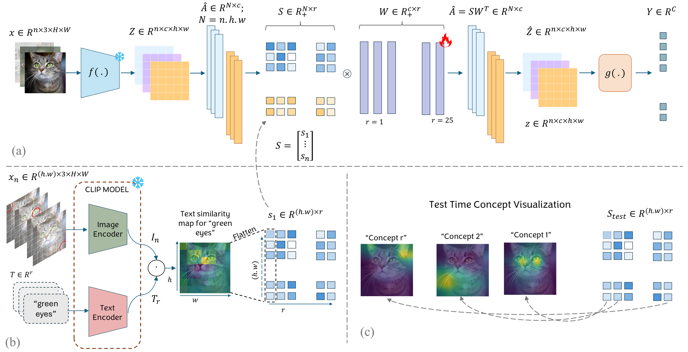
An overview of LAD is shown in Fig. 2. We describe it beginning with the problem setup.
3.1 Setup↩︎
A pretrained model maps inputs from an image space \(\mathcal{X}\subset\mathbb{R}^{3\times H\times W}\) to predictions in \(\mathcal{Y}\subset\mathbb{R}^{c}\). We decompose it into an encoder \(f:\mathcal{X}\rightarrow\mathbb{R}^{p\times h\times w}\) that produces spatial feature maps and a classifier head \(g:\mathbb{R}^{p}\rightarrow\mathbb{R}^{c}\) on globally pooled features. Both remain frozen: LAD explains the deployed model without retraining. For a batch of \(n\) inputs \(\mathbf{X}\), the encoder produces \[\mathbf{Z}=f(\mathbf{X})\in\mathbb{R}^{n\times p\times h\times w},\] where \(p\) is the channel dimension and \((h,w)\) the spatial resolution. Global average pooling (GAP) over the spatial dimensions yields sample-wise latents, with predictions \(g(\mathbf{A})\): \[\mathbf{A}=\operatorname{GAP}(\mathbf{Z})\in\mathbb{R}^{n\times p}.\]
Post-hoc Concept Discovery: Given a frozen model \(g \circ f\), post-hoc concept discovery seeks a low-dimensional, non-negative factorization of the latents \(\mathbf{A}\) into a small set of interpretable components. Most methods operate on pooled activations \(\mathbf{A}\), restricting analysis to a single class to avoid cross-class confounds. Non-negative Matrix Factorization (NMF) is the common formulation: \[\mathbf{A} \;\approx\; \mathbf{U}\mathbf{W}^{\top}, \qquad \mathbf{U}\in\mathbb{R}^{n\times r}_{+},\;\; \mathbf{W}\in\mathbb{R}^{p\times r}_{+},\] where \(r\) is the number of concepts. Each column of \(\mathbf{W}\) defines a concept direction in feature space, and the matching column of \(\mathbf{U}\) its per-sample activation strength. Reconstructed features \(\widehat{\mathbf{A}}=\mathbf{U}\mathbf{W}^{\top}\) can be passed through \(g(\cdot)\) to assess predictive consistency.
3.2 Semantically Anchored Matrix Factorization↩︎
Unlike methods that factorize globally pooled representations \(\mathbf{A}\in\mathbb{R}^{n\times p}\), we factorize directly in the encoder’s spatial feature space to preserve localized evidence. We unfold the activations \(\mathbf{Z}\) over spatial and batch dimensions: \[\bar{\mathbf{A}} = \operatorname{Unfold}(\mathbf{Z}) \in \mathbb{R}^{(n h w)\times p},\] so each row is a spatial location and each column a feature channel. Pooling before factorization implicitly assumes concepts are spatially homogeneous across an image; unfolding instead treats each location as an independent observation, raising the effective sample size from \(n\) to \(n h w\) and capturing localized, part-level structure that pooling would average out. Concept discovery thus becomes a structured clustering over spatial feature vectors while remaining consistent with the classifier’s global decision pipeline.
Inverting the Coefficient Matrix: Standard NMF, \(\mathbf{A} \approx \mathbf{U}\mathbf{W}^{\top}\), learns both \(\mathbf{U}\) and \(\mathbf{W}\), so the coefficients \(\mathbf{U}\) are unconstrained and lack semantic alignment. We invert this: rather than discovering factors and labeling them afterward, we fix the coefficients to a semantically grounded matrix \(\mathbf{S}\) from language–vision similarity and learn only the basis, \[\hat{\bar{\mathbf{A}}} \approx \mathbf{S}\mathbf{W}^{\top}, \qquad \mathbf{S}\in\mathbb{R}_{+}^{(n h w)\times r}.\] Each column of \(\mathbf{S}\) is a human-interpretable concept and each entry the similarity between a spatial location and a concept prompt. This turns factorization into a semantically constrained reconstruction: we learn a basis \(\mathbf{W}\) that best reconstructs encoder activations under fixed, language-aligned coefficients. Because the concept identity is fixed a priori by \(\mathbf{S}\), each basis vector is tied to a named concept, and naming becomes a structural property of the factorization rather than a post-hoc step.
3.3 Language-Anchored Concept Map Construction↩︎
Class-Specific Concept Vocabulary: For each class \(c \in \mathcal{C}\) we build a fixed-size vocabulary \(\mathcal{T}_c = \{t_1,\dots,t_r\}\) of visually grounded concepts (\(r=25\) unless noted; sensitivity in 5.5). Following [10], we prompt a large language model with structured templates eliciting diverse attributes (object parts, textures, shapes, materials, poses, contextual cues). Automatic filtering removes (i) generic filler terms (e.g., “object”), (ii) concepts overlapping the class name (preventing trivial leakage), and (iii) near-duplicates by CLIP text-embedding similarity, yielding a compact, diverse vocabulary with no manual annotation. Templates and filtering details are in the supplement.
Localized CLIP Similarity Maps: Given an image \(x_n\) and its vocabulary \(\mathcal{T}_c\), we construct spatial concept maps via localized prompting [11], [24]. After CLIP’s deterministic preprocessing, we define a grid aligned to \((h,w)\) and, at each location, form a variant \(x_n^{(h,w)}\) by overlaying a small red circle. With \(\ell_2\)-normalized CLIP encoders \(E_I,E_T\), the cosine similarity for concept \(t_m\) is \[s_{n,m}^{(h,w)} = \frac{ E_I(x_n^{(h,w)}) \cdot E_T(\texttt{`a photo of } t_m \texttt{'}) }{ \|E_I(x_n^{(h,w)})\|_2 \, \|E_T(\texttt{`a photo of } t_m \texttt{'})\|_2 }.\] This gives a spatial map \(s_{n,m} \in \mathbb{R}^{h \times w}\); flattening yields \(\mathbf{s}_n \in \mathbb{R}^{(h w)\times r}\) per image, and stacking across images forms the fixed coefficient matrix \[\mathbf{S} = [\,\mathbf{s}_1;\dots;\mathbf{s}_n\,] \in \mathbb{R}^{(n h w)\times r},\] whose rows are spatial locations and columns named concepts, used in the reconstruction \(\hat{\bar{\mathbf{A}}} \approx \mathbf{S}\mathbf{W}^{\top}\).
3.4 Activation-Level Reconstruction Optimization↩︎
With \(\mathbf{S}\) fixed, we recover the concept basis by minimizing the reconstruction error \[\min_{\mathbf{W} \ge 0} \;\mathcal{L}_{\text{recon}} = \frac{1}{2}\|\bar{\mathbf{A}} - \mathbf{S}\mathbf{W}^\top\|_F^2. \label{eq:recon95loss}\tag{1}\] Since GAP is linear and the head reads only pooled features, a small reconstruction error in \(\bar{\mathbf{A}}\) bounds the perturbation of \(\mathbf{A}\), and hence of the logits; empirically, minimizing Eq. 1 alone preserves accuracy across datasets and backbones without output-level regularization. Unlike prior approaches that jointly learn both factors or regularize logits, we fix \(\mathbf{S}\) and learn only \(\mathbf{W}\), enforcing semantic alignment structurally rather than through auxiliary losses.
We optimize Eq. 1 with projected gradient descent (PGD) to enforce non-negativity: \[\mathbf{W} \leftarrow \max(0, \mathbf{W} - \eta \nabla_{\mathbf{W}}\mathcal{L}_{\text{recon}}),\] initialized with NNDSVD [25]. With \(\mathbf{S}\) fixed the objective is smooth in \(\mathbf{W}\) and PGD converges to a stationary point (supplement).
3.5 Inference via Non-Negative Semantic Coefficient Estimation↩︎
With the basis \(\mathbf{W}\) learned, we explain a new image \(x\) against the same frozen encoder. We extract and unfold its activations to \(\bar{\mathbf{A}} \in \mathbb{R}^{(h w)\times p}\) and, with \(\mathbf{W}\) fixed, estimate non-negative coefficients \(\hat{\mathbf{S}} \in \mathbb{R}^{(h w)\times r}_{+}\) by non-negative least squares: \[\min_{\hat{\mathbf{S}} \ge 0} \frac{1}{2} \left\| \hat{\mathbf{S}}\mathbf{W}^{\top} - \bar{\mathbf{A}} \right\|_F^2. \label{eq:nnls95inference}\tag{2}\] A fast non-negative initialization is the projected normal equation \[\hat{\mathbf{S}}_0 = \operatorname{ReLU}\!\left( \bar{\mathbf{A}}\mathbf{W}(\mathbf{W}^{\top}\mathbf{W})^{-1} \right),\] optionally refined by projected gradient descent, \[\hat{\mathbf{S}} \leftarrow \operatorname{ReLU}\!\left( \hat{\mathbf{S}} - \eta(\hat{\mathbf{S}}\mathbf{W}^{\top}\mathbf{W} - \bar{\mathbf{A}}\mathbf{W}) \right),\] with \(\eta\) from the spectral norm of \(\mathbf{W}^{\top}\mathbf{W}\). The reconstruction \(\hat{\bar{\mathbf{A}}}=\hat{\mathbf{S}}\mathbf{W}^{\top}\) is then reshaped and passed through the head after pooling; predictive preservation is the accuracy of the original versus reconstructed activations.
3.6 Concept Heatmaps and Visualization↩︎
We project the inferred coefficients back to the spatial domain. Reshaping \(\hat{\mathbf{S}}\) to \(\hat{\mathbf{S}}_{\text{spatial}} \in \mathbb{R}^{h \times w \times r}\), each concept \(k\) gives a normalized heatmap \[\mathbf{M}_k = \mathrm{Normalize}\!\left(\hat{\mathbf{S}}_{\text{spatial}}(:,:,k)\right),\] rescaled to \([0,1]\), highlighting regions whose features are best reconstructed by the \(k\)-th basis vector. Overlaid on the image, and since channel \(k\) corresponds to the named concept \(t_k\) (e.g., “pointy ears”), each map is a semantically grounded explanation of localized evidence.
4 Experimental Setup↩︎
Datasets: We evaluate LAD on ImageNet (ILSVRC 2012) using a publicly available pretrained ResNet34, analyzing 500 of the 1,000 classes, a substantial expansion over prior concept-discovery work that reports on as few as 10 classes [8]. For scene-centric generalization we use Places365-Standard with the publicly available pretrained ResNet50 checkpoint, covering 364 of 365 categories (one excluded due to \(0\%\) baseline accuracy). We also evaluate a clinical domain (5.4); additional analyses, including results on further CNN backbones and a Vision Transformer case study, are provided in the supplementary material.
Baselines: We compare against representative NMF-based concept discovery methods: ICE [7], CRAFT [5], and FACE [8], all using identical backbones, preprocessing, data splits, and concept counts \(r\).
Metrics: Acc is top-1 agreement between predictions on original and reconstructed activations. C-Ins (\(\uparrow\)) measures whether concepts are sufficient for the decision (performance restored as top concepts are inserted), and C-Del (\(\uparrow\)) whether they are necessary (performance degraded as they are removed).
5 Results↩︎
5.1 Named Concepts and Per-Image Rollouts↩︎
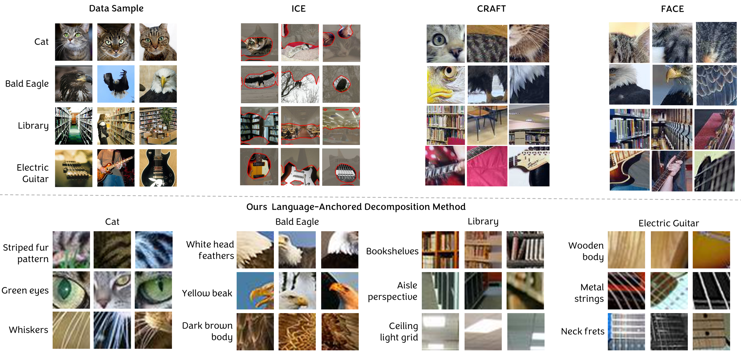
Because LAD anchors each factor to a language-defined concept, a concept refers to the same entity wherever it appears: maple neck, fretted scale, and tuning pegs localize to the same parts across every image of the Electric Guitar class. NMF baselines (ICE, CRAFT, FACE) recover unnamed factors, so the same factor index may highlight the guitar body in one image and the fretboard in another, limiting cross-image comparability [26], [27]. 3 contrasts the two: baseline factors highlight coarse or discriminative regions with no name, whereas LAD recovers fine-grained concepts each tied to a human-interpretable label.
This naming enables a capability no baseline provides: the per-image named-concept rollout. For a single input, LAD returns the named concepts the model used, each localized, ranked by importance, and annotated with its contribution to the reconstruction, \[\hat{c}_k \;=\; \frac{\lVert \hat{\mathbf{S}}[:,k]\rVert_2\,\lVert \mathbf{W}[:,k]\rVert_2}{\sum_{j} \lVert \hat{\mathbf{S}}[:,j]\rVert_2\,\lVert \mathbf{W}[:,j]\rVert_2}, \label{eq:contribution}\tag{3}\] the share of the reconstruction explained by concept \(k\); the baselines can only emit “factor 1, factor 2, …” for a human to label afterward. 4 (top) shows this for an electric guitar and an axolotl: LAD returns localized, named concepts with their contributions, while FACE returns factors of comparable contribution but no semantic label.
Naming also yields cross-image consistency that unnamed factors lack. 4 (bottom) tracks one LAD concept, maple neck, against FACE’s leading factor across several images of the class: the named concept localizes to the neck in every image, whereas the unnamed factor attaches to a different region each time, so its meaning cannot be read off the index. The rollout is thus the per-image, named view of the structure our aggregate metrics summarize (¿tbl:tab:main95comparison?): the concepts it surfaces are those whose insertion and deletion move the prediction.
12pt
l *3S[table-format=1.3] Method & Acc \(\uparrow\) & C-Ins \(\uparrow\) & C-Del \(\uparrow\)
& 1.000 & 0.973 & 0.902
FACE & 0.998 & 0.952 & 0.939
CRAFT & 0.976 & 0.918 & 0.808
ICE & 0.997 & 0.907 & 0.545
& 1.000 & 0.972 & 0.880
FACE & 0.994 & 0.925 & 0.919
CRAFT & 0.947 & 0.868 & 0.828
ICE & 0.995 & 0.887 & 0.631

5.2 Predictive Preservation and Faithful Attribution↩︎
¿tbl:tab:main95comparison? reports our primary comparison. All methods preserve accuracy on both ResNet backbones, with LAD highest, so the semantic constraints do not distort the classifier’s representations; with Acc saturated, faithfulness is read from insertion and deletion. LAD attains the highest C-Ins on both datasets, so its named concepts are the most efficient at restoring the prediction. On C-Del, FACE is strongest. This ordering reflects a design difference, not a deficiency: FACE jointly optimizes coefficients and basis against classifier logits, absorbing any decision-relevant direction including non-interpretable ones, whereas LAD fixes the coefficients to named concepts and recovers a semantically constrained subset of decision-relevant evidence. Trading a portion of deletion completeness for named, verifiable concepts is the intended behavior, and the gap narrows as the concept budget grows (5.5).
Computational cost: LAD is also cheaper to fit than the jointly-optimized baselines. Fixing \(\mathbf{S}\) reduces concept learning to a single non-negative least-squares solve for \(\mathbf{W}\), avoiding the alternating factor updates of CRAFT and the logit-regularized optimization of FACE. On an RTX A4500, LAD fits a class in \(0.03\) s, versus \(0.5\) s (CRAFT) and \(2.6\) s (FACE); a one-time LLM concept generation step adds \({\sim}15\) s/class. A full complexity and wall-clock analysis is in the supplement.
5.3 The Model’s Geometry Determines Retained Concepts↩︎
A central claim of LAD is that the frozen encoder, not CLIP, determines which named concepts survive. 6 provides direct evidence: before optimization, concept scores reflect the CLIP initialization and rank relatively uniformly; after optimizing the basis against encoder activations, the distributions disperse as coefficients are reshaped to reconstruct the model’s internal features. Concepts inconsistent with the encoder’s evidence receive small basis weight and are suppressed, so LAD retains only concepts causally aligned with the decision, which matters given known biases in CLIP-style models [28].
5.4 Concepts in a Clinical Domain↩︎
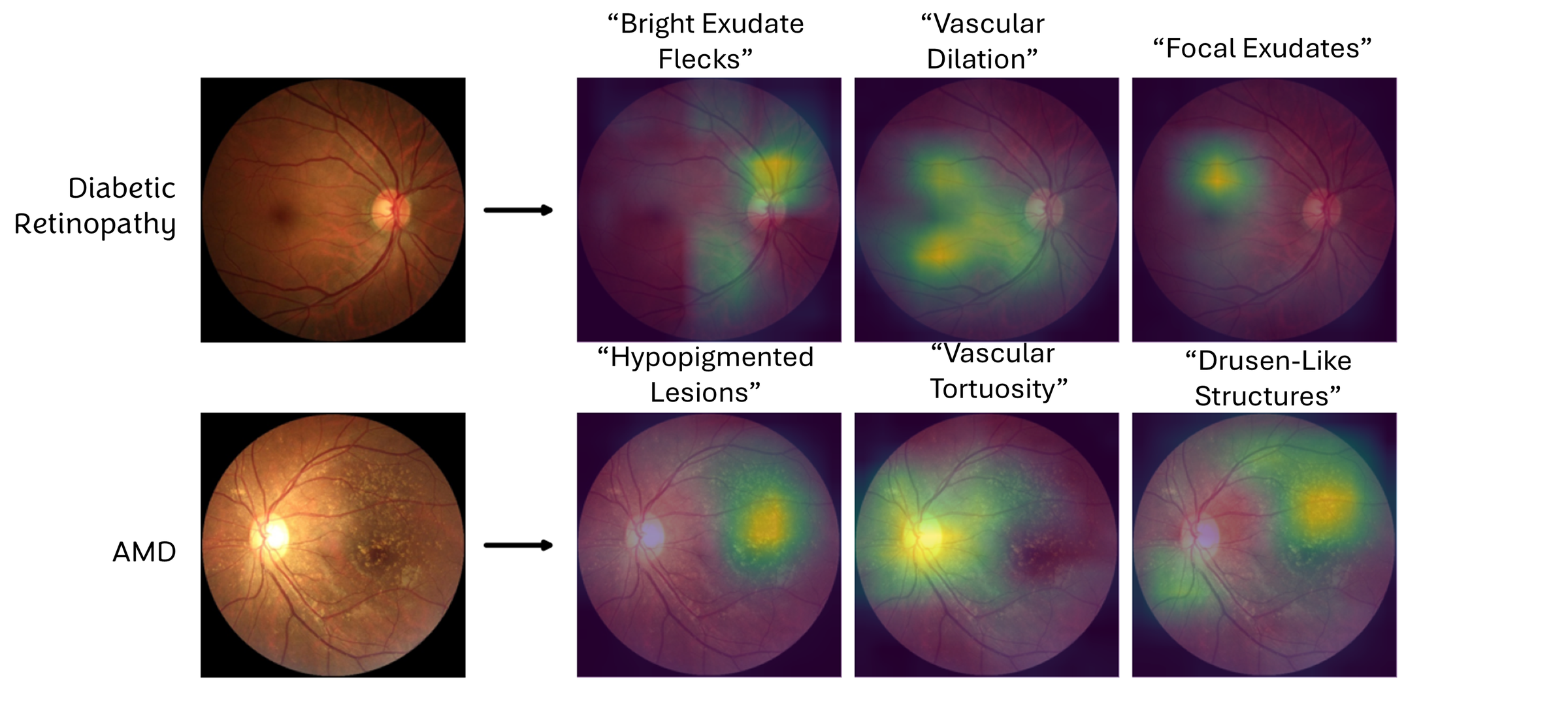
To test whether LAD produces decision-relevant named concepts where interpretability carries real stakes, we evaluate on retinal fundus photographs (ODIR-5K, five ocular-disease classes). The explained model is a DenseNet-121 fine-tuned to \(0.755\) balanced accuracy; per-class vocabularies are generated as disease-specific attributes (e.g., bright exudate flecks, vascular dilation, drusen-like structures) and localized with BiomedCLIP. Dataset and training details are in the supplement.
As on natural images, Acc and C-Ins saturate, so faithfulness is read from deletion (C-Del), where LAD is the most causally decisive of any method (¿tbl:tab:retina?). Unlike the natural-image setting, where FACE’s joint optimization edges out LAD on deletion, the clinical backbone’s evidence is spatially focal: disease signatures occupy small, localized regions rather than distributed texture. LAD’s named concepts anchor to these regions, so removing them degrades the prediction more sharply, and LAD leads C-Del by a wide margin (\(0.954\) vs.\(0.863\)). This aligns with our central finding that the encoder’s geometry, not the language prompts, determines which concepts are retained (5.3): focal disease evidence aligns with named anatomical concepts.
5 shows the qualitative counterpart. For diabetic retinopathy, LAD separates the prediction into named concepts localized to distinct regions; for age-related macular degeneration, drusen-like structures localizes to the yellow deposits temporal to the optic disc, a hallmark of the disease. Because each map carries a clinical name, a reader inspects not only where the model looks but what it attributes there, and can flag when the two disagree, making the rollout an auditable record of the model’s evidence rather than an unlabeled saliency map.
18pt
l *3S[table-format=1.3] Method & Acc & C-Ins & C-Del
(ours) & 1.000 & 0.980 & 0.954
FACE & 0.990 & 0.980 & 0.863
CRAFT & 1.000 & 0.980 & 0.850
ICE & 0.990 & 0.980 & 0.455
5.5 Ablation Studies↩︎
The language anchor: ¿tbl:tab:language95ablation? replaces the fixed language-grounded coefficients \(\mathbf{S}\) with learned ones (standard unsupervised NMF on the same \(\bar{\mathbf{A}}\)). Accuracy is unchanged, but removing the anchor collapses deletion faithfulness, dropping C-Del from \(0.902\) to \(0.507\). The anchor changes which basis directions are discovered, steering them toward classifier-meaningful structure that a purely data-driven factorization does not recover.
Effect of concept budget \(r\): ¿tbl:tab:rank95ablation? varies the number of concepts per class. Accuracy is saturated at all \(r\), while C-Ins and C-Del improve monotonically: a larger vocabulary yields a more expressive basis that remains predictively faithful. We fix \(r=25\) in the main experiments to match the baselines’ budgets; larger \(r\) trades a modest gain in deletion faithfulness for reduced per-image interpretability.
8pt
l *3S[table-format=1.3] Variant & Acc & C-Ins & C-Del
(fixed \(\mathbf{S}\)) & 1.000 & 0.973 & 0.902
Unsupervised NMF on \(\bar{\mathbf{A}}\) & 1.000 & 0.942 & 0.507
\(\Delta\) (language) & — & \(+0.031\) & \(+0.395\)
10pt
ccccblccccrmccccccc *3S[table-format=1.3] ccccblccccrmccccccc & Acc \(\uparrow\) & C-Ins \(\uparrow\) &
C-Del \(\uparrow\) & MSE \(\downarrow\)
& 1.000 & 0.941 & 0.860 & 1.477
25 & 1.000 & 0.973 & 0.902 & 1.483
50 & 1.000 & 0.985 & 0.953 & 1.543
100 & 1.000 & 0.992 & 0.956 & 1.382

6 Conclusion↩︎
We introduced LAD, a post-hoc framework that produces concepts which are simultaneously named, faithful, and obtained without modifying the model. By inverting non-negative matrix factorization, fixing CLIP-derived language-grounded coefficients and learning only the concept basis against the frozen encoder, LAD ties each basis direction to a human-readable concept while preserving the model’s predictive behavior. Removing the language anchor preserves accuracy but collapses faithfulness, showing that the anchor determines which concept directions are discovered rather than merely labeling them.
Across ImageNet and Places365, LAD matches the strongest prior method on faithfulness while uniquely supporting per-image named-concept rollouts: for a single input, the named concepts the model relied on, each localized and annotated with its contribution. On retinal fundus images its named concepts are the most causally decisive of any method, showing the approach carries to a high-stakes clinical domain. By making a model’s semantic evidence directly inspectable and comparable across images, LAD supports more transparent vision models where understanding the content of a decision matters as much as its accuracy.
Supplementary Material
6.0.0.1 Organization.
This supplementary material provides additional implementation details, theoretical analysis, and extended results supporting the main paper.
Sec. 7 describes the construction of the class-specific concept vocabularies via LLM generation and semantic filtering, and the CLIP-based spatial probing used to build concept maps (Sec. 7.6).
Sec. 8 gives the optimization solver details deferred from the main paper.
Sec. 9 provides the convergence analysis for the projected gradient descent procedure.
Sec. 10 evaluates four additional ImageNet backbones, including a robustness analysis on a lightweight network.
Sec. 11 reports a second clinical domain (dermoscopy) and an analysis of where the discovered concepts localize.
Sec. 12 reports a per-stage computational cost and memory analysis against the baselines.
Sec. 13 presents a Vision Transformer case study.
Sec. 14 shows extended qualitative visualizations of discovered concepts.
Sec. 15 provides additional qualitative comparisons with ICE, CRAFT, and FACE.
7 Class-Specific Concept Vocabulary Generation↩︎
For each target class, we construct a fixed vocabulary of 25 visually grounded concepts that serve as the semantic basis for our concept maps. The vocabulary is generated using a constrained large language model (LLM) pipeline followed by lexical and CLIP-based semantic filtering.
7.1 Prompt Design↩︎
Concept proposals are generated using the gpt-4o-mini model. The system prompt instructs the model to generate short, visually grounded descriptors suitable for interpretability analysis. The user prompt specifies the target ImageNet class
and enforces several constraints:
Exactly 25 concepts must be generated.
Each concept must contain 2–3 lowercase words.
Concepts must describe visually grounded attributes such as parts, textures, shapes, contexts, or actions.
The class name and trivial synonyms are disallowed.
Previously rejected or accepted concepts are added to a banned list to encourage diversity across iterations.
Example prompt template:
Generate EXACTLY 25 distinct visual
concepts for the ImageNet class:
"{class_name}". Concepts must be 2-3
words, lowercase, visually grounded.
Avoid the class name or synonyms.
Avoid generic words such as "object",
"scene", "photo". Return JSON only.
7.2 Schema-Constrained Generation↩︎
To ensure structured, reproducible outputs, generation is constrained by a strict JSON schema: the output must contain the class name and exactly 25 concept strings, \[\label{eq:concept95schema} \texttt{schema} = \left\{ \begin{array}{l} \texttt{class\_name}: \text{string} \\ \texttt{concepts}: [c_1, \dots, c_{25}], \quad c_i \in \mathcal{S}, \end{array} \right.\tag{4}\] where each concept \(c_i\) is a 2–3 word lowercase phrase of 3–40 characters matching the pattern
[a-z][a-z-]*([ ][a-z][a-z-]*){1,2}This guarantees the LLM returns exactly 25 short, controlled-format concepts.
7.3 Stage-1 Lexical Filtering↩︎
Raw LLM outputs are normalized through lowercasing and removal of non-alphabetic characters. A rule-based filter then removes concepts that violate the following conditions:
Not 2–3 words long
Contain generic filler terms (e.g., animal, object, scene)
Duplicate previously accepted concepts
Contain tokens identical to the class name
To avoid removing meaningful attributes, we maintain a lexicon of visual attribute words spanning several categories:
color (e.g., yellow, black)
texture (e.g., furry, shiny)
parts (e.g., tail, wings)
shape (e.g., long, round)
pose/motion (e.g., running, flying)
environment (e.g., forest, ocean)
material (e.g., metal, wood)
Concepts containing attribute words are preserved even if partial lexical overlap with the class name occurs.
7.4 Stage-2 CLIP Semantic Filtering↩︎
After lexical filtering, we apply a CLIP-based semantic filtering procedure to improve diversity and visual relevance.
Let \(t_i\) denote the CLIP text embedding of concept \(c_i\) obtained using the template:
\[\text{``a photo of } c_i \text{''}.\]
If class images are available, we randomly sample up to 100 images from the target class and compute their CLIP image embeddings. The mean embedding
\[\mu_I = \frac{1}{N}\sum_{j=1}^{N} f_{\text{CLIP}}(I_j)\]
serves as a prototype representation of the class.
Concepts are ranked by cosine similarity
\[s_i = \langle t_i, \mu_I \rangle .\]
To preserve semantic diversity, concepts are greedily selected while enforcing
\[\max_{k < i} \langle t_i, t_k \rangle < 0.80 .\]
This removes near-duplicate concepts in the CLIP embedding space while favoring those that align with the visual distribution of the class.
7.5 Iterative Generation Procedure↩︎
7 summarizes vocabulary generation. Early rounds apply both lexical and CLIP-based filtering to encourage visual relevance and diversity. If a class has not reached 25 concepts after the CLIP-filtered rounds, later rounds disable CLIP pruning and keep only the lexical constraints, guaranteeing exactly 25 valid concepts per class.

7.6 CLIP-Based Concept Map Construction↩︎
After constructing the class-specific concept vocabulary (Sec. 7), we use CLIP to localize each concept within an image and build spatial concept maps. The goal is to measure how strongly each concept aligns with different spatial regions of the image.
7.6.0.1 CLIP model.
We use a pretrained CLIP vision–language model to compute similarity between image regions and concept text prompts. In our implementation we use the ViT-B/16 architecture, loaded either through the open_clip library with pretrained weights
(e.g., laion2b_s34b_b88k) or the original OpenAI CLIP implementation when open_clip is unavailable. All image and text features are \(\ell_2\) normalized before computing cosine similarity.
7.6.0.2 Concept text embeddings.
For each concept \(c_i\) in the vocabulary of size \(M=25\), we construct a CLIP text prompt using the template
\[t_i = \text{``a photo of } c_i \text{''}.\]
The CLIP text encoder produces a normalized embedding
\[\mathbf{t}_i = f_{\text{text}}(t_i) \in \mathbb{R}^{D}.\]
All text embeddings are precomputed and cached to avoid redundant computation during image processing.
7.6.0.3 Spatial probing via localized prompts.
To obtain spatially localized responses, we probe the image using a grid of visual prompts. Each input image is first resized and center-cropped to the standard CLIP resolution of \(224 \times 224\). We then define a uniform grid of \(H_t \times W_t\) spatial locations (typically \(7 \times 7\)). For each grid cell center, we overlay a thin red circular outline with fixed radius \(r\) on the image.
This produces a set of \(H_t W_t\) modified images:
\[\{ I_{p} \}_{p=1}^{H_t W_t},\]
where each \(I_p\) highlights a different spatial location through the circle prompt.
Each prompted image is encoded by the CLIP image encoder:
\[\mathbf{v}_p = f_{\text{img}}(I_p) \in \mathbb{R}^{D}.\]
The resulting features are also \(\ell_2\) normalized.
7.6.0.4 Concept similarity maps.
For each spatial location \(p\) and concept \(i\), we compute the cosine similarity between the image embedding and the concept embedding:
\[S_{p,i} = \mathbf{v}_p^\top \mathbf{t}_i .\]
Optionally, the similarity scores are scaled by the CLIP temperature parameter \(\exp(\text{logit\_scale})\).
The resulting similarity tensor
\[S \in \mathbb{R}^{H_t W_t \times M}\]
is reshaped into a spatial concept map
\[P_i \in \mathbb{R}^{H_t \times W_t}\]
for each concept \(i\). The stack of maps
\[P = \{P_i\}_{i=1}^{M}\]
represents the spatial activation of all concepts across the image.
8 Optimization Details↩︎
This section gives the solver details for the basis-learning objective (Eq. 1) and the inference problem (Eq. 3) in the main paper.
Basis update. We enforce non-negativity in Eq. 1 with the projected gradient step \[\mathbf{W} \leftarrow \max\!\big(0,\;\mathbf{W} - \eta \nabla_{\mathbf{W}}\mathcal{L}_{\text{recon}}\big), \label{eq:supp95pgd95w}\tag{5}\] initialized with NNDSVD [25] for stable, accelerated convergence. With \(\mathbf{S}\) fixed, \(\mathcal{L}_{\text{recon}}\) is a smooth quadratic in \(\mathbf{W}\), so projected gradient descent converges to a stationary point.
Inference solver. For the inference problem (Eq. 3), a fast non-negative initialization is the projected normal equation \[\hat{\mathbf{S}}_0 = \operatorname{ReLU}\!\left(\bar{\mathbf{A}}\mathbf{W}(\mathbf{W}^{\top}\mathbf{W})^{-1}\right), \label{eq:supp95normal95eq}\tag{6}\] optionally refined by projected gradient descent, \[\hat{\mathbf{S}} \leftarrow \operatorname{ReLU}\!\left(\hat{\mathbf{S}} - \eta(\hat{\mathbf{S}}\mathbf{W}^{\top}\mathbf{W} - \bar{\mathbf{A}}\mathbf{W})\right), \label{eq:supp95pgd95s}\tag{7}\] where the step size \(\eta\) is set from the spectral norm of \(\mathbf{W}^{\top}\mathbf{W}\).
Heatmap normalization. For visualization, each concept channel is rescaled to \([0,1]\), \[\mathbf{M}_k = \mathrm{Normalize}\!\left(\hat{\mathbf{S}}_{\text{spatial}}(:,:,k)\right). \label{eq:supp95heatmap}\tag{8}\]
9 PGD Convergence Analysis↩︎
We analyze the convergence of the projected gradient descent (PGD) procedure used to optimize the activation-level reconstruction objective introduced in Sec. 3.4 of the main paper. In our formulation the semantic coefficient matrix \(\mathbf{S}\) is fixed, and we learn only the nonnegative concept basis \(\mathbf{W}\).
Let \(\bar{\mathbf{A}} \in \mathbb{R}^{N \times p}\) denote the unfolded encoder activations, where \(N = n h w\) corresponds to the number of spatial locations across all images. The matrix \(\mathbf{S} \in \mathbb{R}^{N \times r}\) represents the fixed CLIP-derived semantic similarity matrix. The optimization problem for the concept basis \(\mathbf{W} \in \mathbb{R}^{p \times r}_{+}\) is
\[\label{eq:opt95recon} \min_{\mathbf{W} \ge 0} \mathcal{L}(\mathbf{W}) = \frac{1}{2} \|\bar{\mathbf{A}} - \mathbf{S}\mathbf{W}^\top\|_F^2 .\tag{9}\]
This objective enforces activation-level fidelity between the original latent activations \(\bar{\mathbf{A}}\) and the reconstruction \(\mathbf{S}\mathbf{W}^\top\) obtained from the concept coefficients \(\mathbf{S}\) and concept bases \(\mathbf{W}\).
9.0.0.1 Smoothness.
The loss in Eq. 9 is a convex quadratic function of \(\mathbf{W}\). Rewriting the objective as
\[\mathcal{L}(\mathbf{W}) = \frac{1}{2} \|\bar{\mathbf{A}}^\top - \mathbf{W}\mathbf{S}^\top\|_F^2 ,\]
its gradient with respect to \(\mathbf{W}\) is
\[\nabla_{\mathbf{W}} \mathcal{L}(\mathbf{W}) = \mathbf{W}(\mathbf{S}^\top \mathbf{S}) - \bar{\mathbf{A}}^\top \mathbf{S}.\]
Since \(\mathbf{S}^\top\mathbf{S}\) is positive semidefinite, the gradient is Lipschitz continuous with constant
\[L_\nabla = \|\mathbf{S}^\top\mathbf{S}\|_2 .\]
Therefore the objective \(\mathcal{L}(\mathbf{W})\) is \(L_\nabla\)–smooth.
9.0.0.2 Projected gradient update.
To enforce the nonnegativity constraint on \(\mathbf{W}\), we apply projected gradient descent. The update rule is
\[\label{eq:pgd95update} \mathbf{W}_{k+1} = \Pi_{\mathbb{R}_+^{p\times r}} \left( \mathbf{W}_k - \eta \nabla \mathcal{L}(\mathbf{W}_k) \right),\tag{10}\]
where \(\Pi_{\mathbb{R}_+^{p\times r}}(\cdot)\) denotes the Euclidean projection onto the nonnegative orthant, implemented elementwise as \(\max(0,\cdot)\).
9.0.0.3 Descent property.
For an \(L_\nabla\)–smooth function, the standard descent lemma gives
\[\label{eq:descent} \mathcal{L}(\mathbf{W}') \le \mathcal{L}(\mathbf{W}) + \langle \nabla \mathcal{L}(\mathbf{W}), \mathbf{W}'-\mathbf{W} \rangle + \frac{L_\nabla}{2} \|\mathbf{W}'-\mathbf{W}\|_F^2 .\tag{11}\]
Applying Eq. 11 with \(\mathbf{W}' = \mathbf{W}_{k+1}\) and using the optimality condition of the projection step yields
\[\langle \nabla \mathcal{L}(\mathbf{W}_k), \mathbf{W}_{k+1}-\mathbf{W}_k \rangle \le -\frac{1}{\eta} \|\mathbf{W}_{k+1}-\mathbf{W}_k\|_F^2 .\]
Substituting this bound into Eq. 11 gives
\[\mathcal{L}(\mathbf{W}_{k+1}) \le \mathcal{L}(\mathbf{W}_k) - \left( \frac{1}{\eta} - \frac{L_\nabla}{2} \right) \|\mathbf{W}_{k+1}-\mathbf{W}_k\|_F^2 .\]
Therefore, for any step size satisfying
\[0 < \eta < \frac{2}{L_\nabla},\]
the objective decreases monotonically,
\[\mathcal{L}(\mathbf{W}_{k+1}) \le \mathcal{L}(\mathbf{W}_k).\]
9.0.0.4 Convergence.
Because \(\mathcal{L}(\mathbf{W}) \ge 0\), the sequence \(\{\mathcal{L}(\mathbf{W}_k)\}\) is monotonically decreasing and therefore convergent. Furthermore,
\[\|\mathbf{W}_{k+1}-\mathbf{W}_k\|_F \rightarrow 0 .\]
Every accumulation point of the PGD iterates satisfies the first-order optimality condition for Eq. 9 . Since the objective is convex and the feasible set \(\{\mathbf{W} \ge 0\}\) is convex, any such stationary point is a global minimizer of the problem.
10 Additional Backbones↩︎
To test whether LAD’s behavior is consistent across encoder architectures, we evaluate four additional ImageNet backbones spanning different design families: RegNetY-8GF, ResNet-152, ResNeXt-50 (32\(\times\)4d), and MobileNetV3-Large (¿tbl:tab:more95backbones?). All methods use identical preprocessing, data splits, and concept count (\(r{=}25\)).
10.0.0.1 Consistency with the main results.
The pattern matches the main paper. LAD preserves reconstruction accuracy (Acc \(\ge 0.999\) on all four) and attains the highest or tied concept insertion (C-Ins) on every backbone, so its named concepts remain the most efficient at restoring the prediction. On deletion (C-Del), LAD and FACE trade the lead, as on ImageNet and Places365: LAD leads on RegNetY-8GF, while FACE edges it on ResNet-152 and ResNeXt-50. The gap is small in every case, consistent with LAD recovering a named, decision-relevant subset of the evidence FACE absorbs through unconstrained logit alignment.
10.0.0.2 Robustness on a lightweight backbone.
MobileNetV3-Large is the most informative case. LAD remains stable (Acc \(0.999\), C-Ins \(0.962\), C-Del \(0.946\)), whereas CRAFT and FACE degrade sharply and become highly unstable across classes (C-Del \(0.804{\pm}0.25\) and \(0.781{\pm}0.22\) versus LAD’s \(0.946\)). Fixing the coefficients to language-grounded concepts evidently regularizes the decomposition on compact, low-redundancy architectures where the baselines’ jointly-optimized factors do not reliably converge.
5pt
ll *3S[table-format=1.3] Backbone & Method & Acc & C-Ins & C-Del
& & 1.000 & 0.977 & 0.953
& CRAFT & 0.997 & 0.971 & 0.940
& FACE & 0.998 & 0.977 & 0.951
& & 0.999 & 0.975 & 0.914
& CRAFT & 0.995 & 0.971 & 0.867
& FACE & 0.995 & 0.975 & 0.952
& & 1.000 & 0.972 & 0.867
& CRAFT & 0.992 & 0.963 & 0.861
& FACE & 0.992 & 0.974 & 0.961
& & 0.999 & 0.962 & 0.946
& CRAFT & 0.839 & 0.805 & 0.804
& FACE & 0.856 & 0.813 & 0.781
11 Second Clinical Domain: Dermoscopy↩︎
To test whether LAD’s clinical results extend beyond retinal fundus, we add a second medical domain, skin-lesion dermoscopy (HAM10000), explained with the same domain-matched medical CLIP (BiomedCLIP) used for fundus.
11.0.0.1 Setup.
HAM10000 contains \(10{,}015\) dermoscopy images across seven lesion classes, split at the lesion level (all shots of a lesion kept together to prevent leakage) into \(8{,}021\) train /
\(1{,}994\) validation (seed \(42\)). The explained model is a ConvNeXt-Small with an ImageNet-pretrained encoder and a \(768\!\rightarrow\!7\) linear head,
trained at \(224\) then fine-tuned at \(448\) with inverse-frequency-weighted cross-entropy and selected by balanced accuracy, reaching \(0.846\) balanced
accuracy (\(0.878\) top-1). Concepts are generated as in Sec. 7 (25/class, gpt-4o-mini) and localized with BiomedCLIP by red-circle prompting; full setup is in 1.
11.0.0.2 Results.
¿tbl:tab:dermoscopy? reports concept faithfulness on both clinical domains under identical metric code and a matched \(7{\times}7\) probe grid, so differences reflect the concept basis rather than the evaluation. As on retinal fundus, accuracy saturates and LAD leads concept deletion (C-Del), exceeding the strongest baseline on dermoscopy (\(0.418\) vs.CRAFT \(0.366\)); LAD also retains saturated insertion (\(0.980\)) whereas FACE’s drops to \(0.790\). Absolute C-Del, however, is far lower than on fundus (\(0.418\) vs.\(0.954\)) for every method.
11.0.0.3 Where the concepts localize.
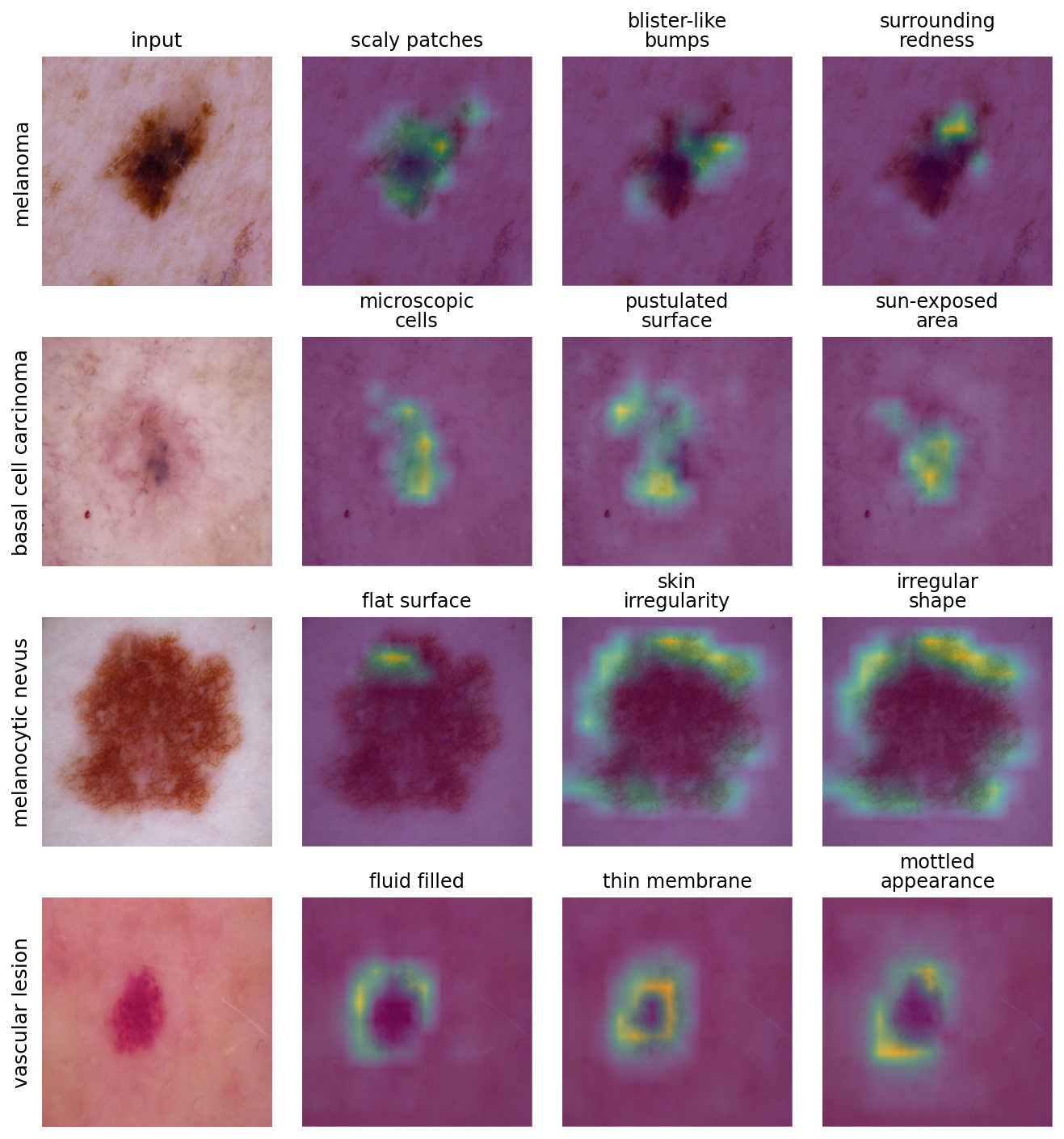
8 explains the lower deletion score. The named concepts localize predominantly to the lesion border and peri-lesional skin rather than to the diagnostic lesion interior. For melanocytic nevus, “skin irregularity” and “irregular shape” form a ring around the lesion edge while the pigmented center stays inactive; for vascular lesion, “fluid filled,” “thin membrane,” and “mottled appearance” encircle the rim; for melanoma, “surrounding redness” and “scaly patches” fall on the margin and adjacent skin. Basal cell carcinoma is the main exception, with concepts landing on the lesion body. This boundary bias and the low C-Del are the same phenomenon: because the discriminative interior texture (pigment network, color variegation) is largely untouched, removing the boundary-localized concepts leaves the evidence the head relies on intact, so the prediction changes little. We report this as a limitation: in this domain LAD’s named concepts are spatially coherent and consistent across images, but they often track lesion shape and context rather than the internal morphology a dermatologist weighs most, so the explanations are better read as localizing where the model’s lesion-level evidence sits than as asserting clinically complete reasoning.
5pt
ll *3S[table-format=1.3] Domain & Method & Acc & C-Ins & C-Del
& & 1.000 & 0.980 & 0.954
& FACE & 0.990 & 0.980 & 0.863
& CRAFT & 1.000 & 0.980 & 0.850
& ICE & 0.990 & 0.980 & 0.455
& & 1.000 & 0.980 & 0.418
& CRAFT & 0.980 & 0.940 & 0.366
& FACE & 0.990 & 0.790 & 0.254
| Retinal | Dermoscopy | |
|---|---|---|
| Dataset | ODIR-5K | HAM10000 |
| Classes | 5 | 7 |
| Train / Val | 3,376 / 843 | 8,021 / 1,994 |
| Backbone | DenseNet-121 | ConvNeXt-Small |
| CLIP | BiomedCLIP | BiomedCLIP |
| Probe grid | \(14{\times}14\) | \(14{\times}14\) |
| PGD steps | 250 | 150 |
| Bal. acc. | 0.755 | 0.846 |
12 Computational Cost↩︎
2 breaks down the per-class cost of LAD on an RTX A4500 (ResNet34, \(r{=}25\)). The recurring concept-learning cost, the basis fit, is \(0.03\) s, an order of magnitude below CRAFT (\(0.5\) s) and FACE (\(2.6\) s), because fixing \(\mathbf{S}\) reduces basis learning to a single non-negative least-squares solve rather than alternating factor updates. Inference is effectively free. The dominant cost is CLIP concept-map construction, a one-time, fully cacheable preprocessing step; the LLM vocabulary is generated once (\(\sim\)15 s/class) and cached.
| Stage | Wall (s) | GPU peak (MB) | ||||||||||||||||||||||||||||||||||||
|---|---|---|---|---|---|---|---|---|---|---|---|---|---|---|---|---|---|---|---|---|---|---|---|---|---|---|---|---|---|---|---|---|---|---|---|---|---|---|
| Activation extraction | 0.01 | 926 | ||||||||||||||||||||||||||||||||||||
| CLIP map construction | 6.45 | 1729 | ||||||||||||||||||||||||||||||||||||
| LLM vocab (one-time) | 15.0 | 0 | ||||||||||||||||||||||||||||||||||||
| fit | 0.03 | 745 | ||||||||||||||||||||||||||||||||||||
| inference | \(<0.01\) | 722 | ||||||||||||||||||||||||||||||||||||
| CRAFT fit | 0.50 | 783 | ||||||||||||||||||||||||||||||||||||
| FACE fit | 2.60 | 795 |
12.0.0.1 CLIP map construction is the bottleneck, and it is bounded.
Concept-map construction probes a \(14{\times}14\) grid of red-circle prompts per image, so its cost scales with the number of CLIP forward passes, not with the decomposition. It is also the only memory-significant stage. 3 shows peak GPU memory as a function of CLIP batch size: the whole pipeline fits in under \(1.8\) GB even at the default batch, with throughput around \(1{,}000\) prompted variants per second. The step is parallel across grid locations and images and is computed once per class, then cached.
| CLIP batch | GPU peak (MB) | Variants/s | ||||||||||||||||||||||||||||||||||||||||||||||||||||||
|---|---|---|---|---|---|---|---|---|---|---|---|---|---|---|---|---|---|---|---|---|---|---|---|---|---|---|---|---|---|---|---|---|---|---|---|---|---|---|---|---|---|---|---|---|---|---|---|---|---|---|---|---|---|---|---|---|
| 16 | 976 | 1158 | ||||||||||||||||||||||||||||||||||||||||||||||||||||||
| 32 | 1045 | 1156 | ||||||||||||||||||||||||||||||||||||||||||||||||||||||
| 64 | 1183 | 988 | ||||||||||||||||||||||||||||||||||||||||||||||||||||||
| 128 | 1450 | 1032 | ||||||||||||||||||||||||||||||||||||||||||||||||||||||
| 196 | 1729 | 970 |
12.0.0.2 Grid sensitivity.
The probe grid sets both the spatial resolution of the concept maps and the cost. 4 compares the \(7{\times}7\) grid (used for ImageNet and dermoscopy) with the \(14{\times}14\) grid (used for the retinal fundus models). The finer grid quadruples the prompted variants per image (\(49\to196\)) and costs roughly \(3.4\times\) the time and \(1.6\times\) the peak memory, the price paid for the higher-resolution localization that focal retinal evidence benefits from.
| Grid | Variants/img | Wall (s, 32 img) | GPU peak (MB) | ||||||||||||||||||||||||||||||||||||||||||||||||||||||
|---|---|---|---|---|---|---|---|---|---|---|---|---|---|---|---|---|---|---|---|---|---|---|---|---|---|---|---|---|---|---|---|---|---|---|---|---|---|---|---|---|---|---|---|---|---|---|---|---|---|---|---|---|---|---|---|---|---|
| \(7{\times}7\) | 49 | 1.88 | 1116 | ||||||||||||||||||||||||||||||||||||||||||||||||||||||
| \(14{\times}14\) | 196 | 6.37 | 1737 |
13 Vision Transformer Case Study↩︎
NMF-style concept discovery (ICE, CRAFT, FACE) is formulated for convolutional feature maps: it factorizes a spatial activation tensor whose channels share a consistent, translation-equivariant geometry. Vision Transformers break both assumptions, they
emit patch tokens rather than a spatial map, mix global information through self-attention at every layer, and route the prediction through a [CLS] token rather than pooled spatial features. Consequently no existing post-hoc concept-discovery
method is designed to operate on both CNNs and ViTs, and the convolutional baselines do not apply to patch tokens at all. Because LAD fixes language-grounded coefficients and learns only a basis, it can be run on ViT patch tokens without
modification, which lets us ask a question the field has not examined: when an anchored decomposition is applied to a transformer, what kind of concepts does it actually recover?
13.0.0.1 Setup.
We decompose the penultimate patch-token representation of ViT-B/16 (\(14{\times}14{\times}768\)) into the language-anchored basis and let the remaining block, LayerNorm, and head complete the forward pass, on the same 500 ImageNet classes (\(r{=}25\)).
13.0.0.2 Reconstruction transfers, but localization does not.
Numerically, the decomposition reconstructs the representation well: reconstruction accuracy and concept insertion are saturated (Acc \(=0.98\), C-Ins \(=0.98\)). Concept deletion,
however, is near zero (C-Del \(=0.02\)). Two factors combine here. First, the head reads from the preserved [CLS] token, which carries information from the original forward pass, so ablating patch-token
concepts has little effect on the logits, and CNN-style deletion is not directly meaningful. Second, and more telling, the recovered concept maps are weakly localized.
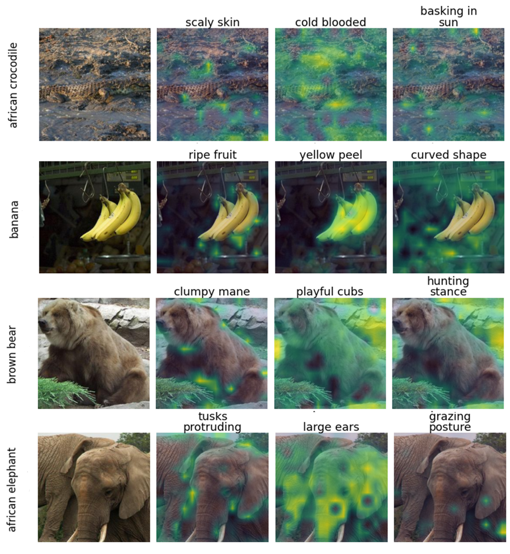
9 makes this visible. On CNNs, LAD localizes named concepts to the corresponding object part (Sec. 5.1, main paper); on ViT, the same concepts spread diffusely and frequently attach to the background or trace the object silhouette rather than the named part. “Cold blooded” for the crocodile activates on the surrounding rock and water; “large ears” on the elephant covers the whole head and contour rather than the ears; the bear’s “hunting stance” and “playful cubs” fire across the entire frame. A few color- or texture-defined concepts do localize (“yellow peel” and “ripe fruit” on the banana), but the part- and pose-level concepts that localize cleanly on CNNs do not. The maps behave closer to global saliency or edge responses than to the part-grounded evidence LAD recovers on convolutional encoders.
13.0.0.3 Takeaway.
This is a negative result, and an informative one: it shows why spatial concept decomposition is not readily transferable to transformers. The patch-token geometry, global attention mixing, and [CLS]-routed prediction together mean
that a language-anchored basis can reconstruct the representation (high insertion) without its concepts being spatially faithful (low deletion, diffuse maps). A transformer-native formulation, operating on the [CLS] attention pathway rather
than patch tokens, and a [CLS]-aware deletion protocol, are needed before concept discovery is meaningful on ViTs; we view this as the natural next step rather than a property of LAD specifically.
l *3S[table-format=1.2] Backbone & Acc \(\uparrow\) & C-Ins \(\uparrow\) & C-Del
ViT-B/16 & 0.98 & 0.98 & 0.02\(^{\dagger}\)
\(\dagger\) Not comparable to CNNs (preserved [CLS] pathway; see text).
14 Visual analysis of concept maps↩︎
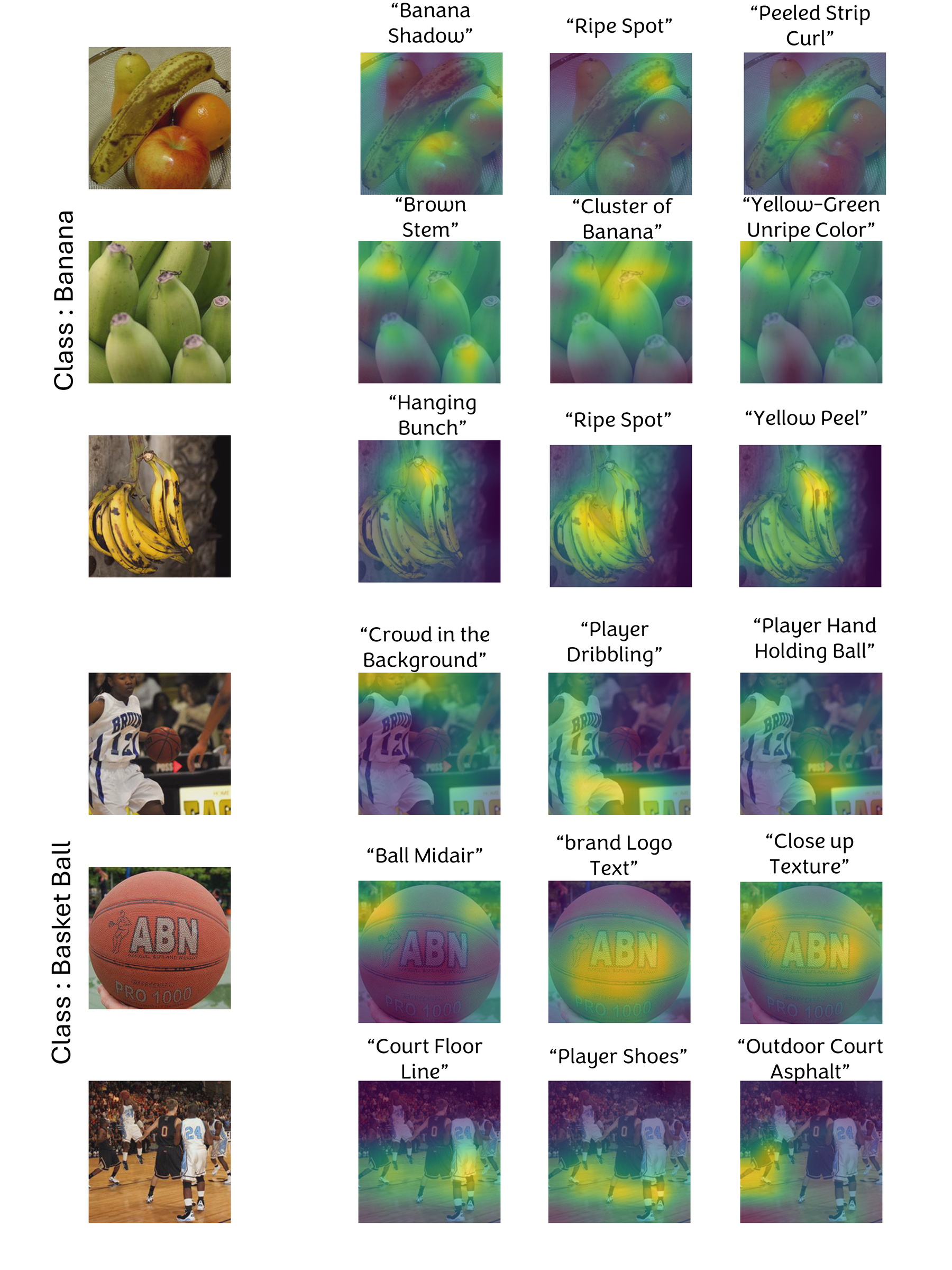
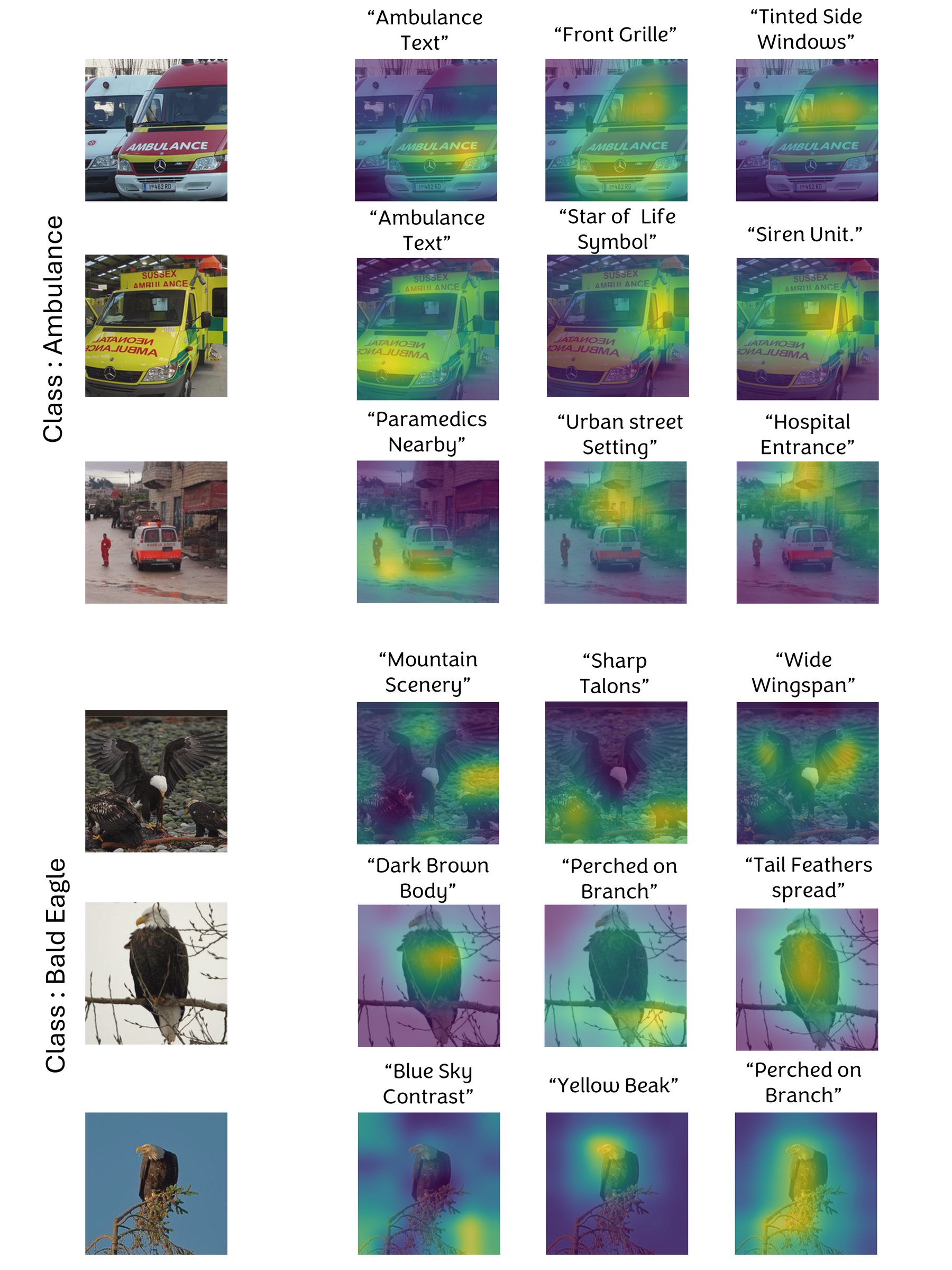
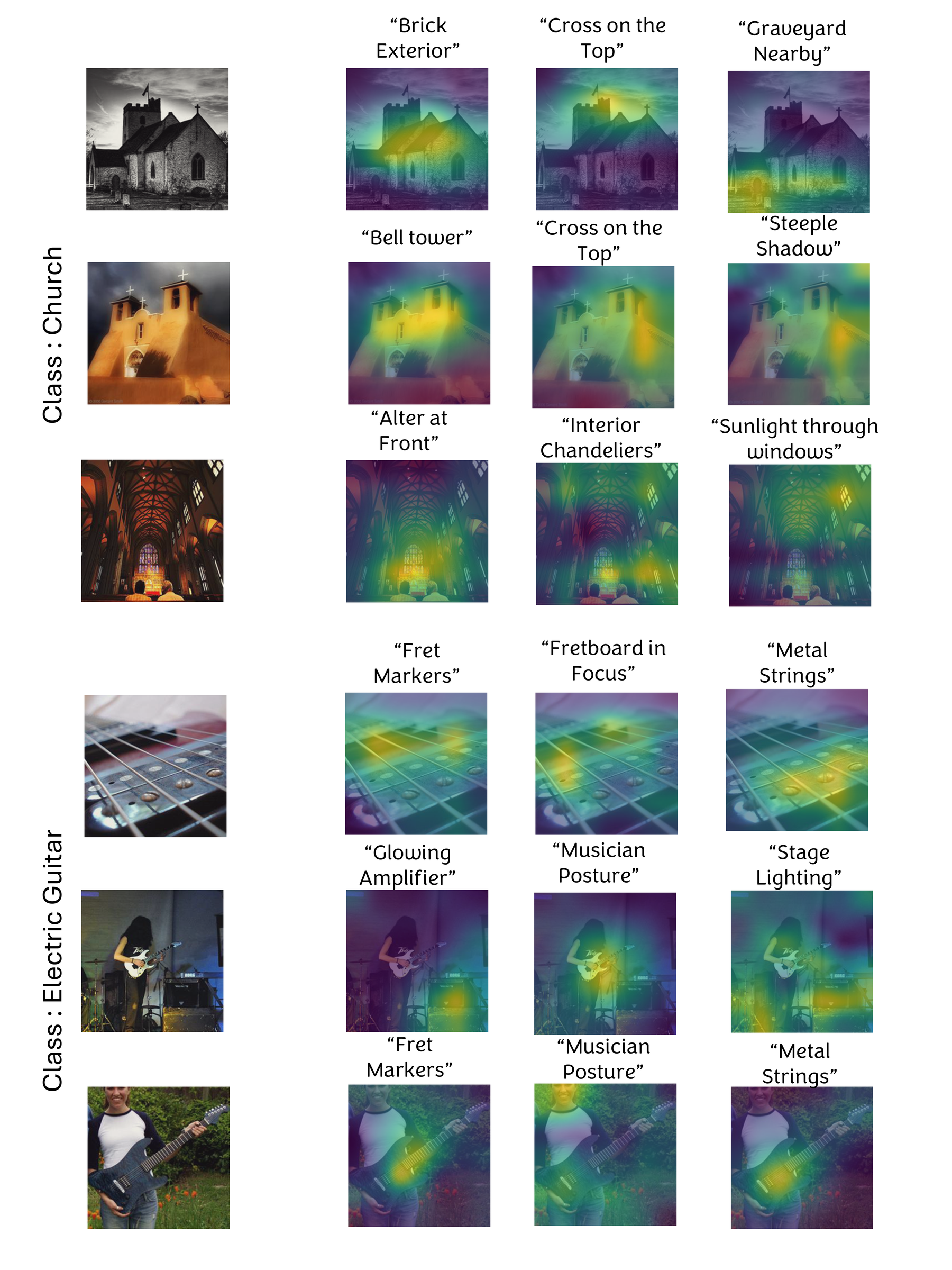
The concept visualizations in Figures 10–12 demonstrate that our method discovers interpretable and spatially grounded concepts across a diverse range of ImageNet categories. For object-centric classes such as Ambulance, the model captures distinctive parts including “Ambulance Text,” “Front Grille,” with heatmaps closely aligned to the corresponding regions of the vehicle. Contextual cues such as “Urban Street Setting” and “Paramedics Nearby” also emerge, reflecting the model’s ability to represent both object parts and scene-level signals.
For natural categories like Bald Eagle, the discovered concepts emphasize fine-grained attributes such as “Sharp Talons,” “Wide Wingspan,” “Tail Feathers Spread,” and “Perched on Branch,” demonstrating that the factorization captures species-dependent morphology and pose-specific details.
The Banana and Basketball classes similarly exhibit semantically coherent concepts: color and ripeness cues (“Ripe Spot,” “Yellow Peel”), cluster structure (“Hanging Bunch”), and environment attributes (“Crowd in the Background,” “Court Floor Line,” “Player Shoes”). These maps show that the method cleanly separates object features from contextual scene information.
Finally, the Church and Electric Guitar classes highlight the model’s ability to encode structural and material properties. Concepts such as “Brick Exterior,” “Bell Tower,” and “Interior Chandeliers” reflect architectural components, while guitar-related concepts such as “Fret Markers,” “Metal Strings,” “Musician Posture,” and “Stage Lighting” localize on instrument parts and performance settings.
Overall, these qualitative results illustrate that the proposed model recovers rich, human-understandable concepts that respect object structure, texture, and scene context, providing spatially faithful explanations without manual labeling.
15 Additional Concept Discovery Comparison↩︎
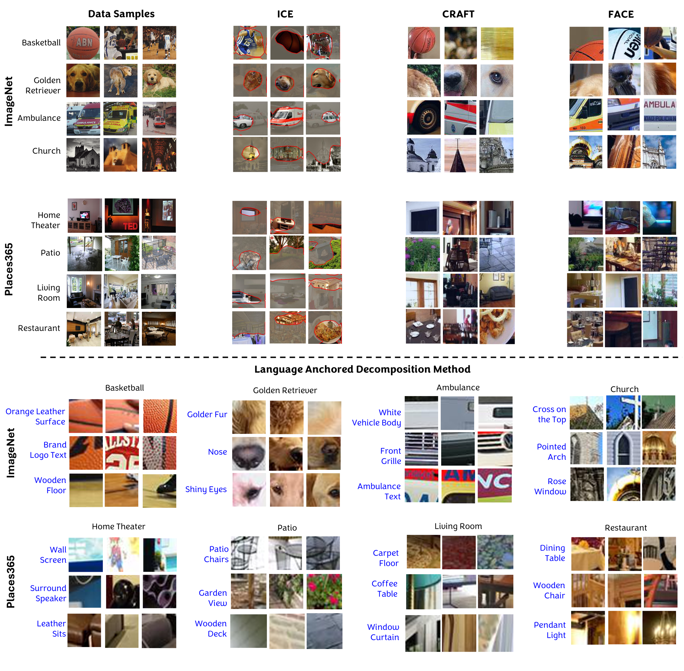
Figure 13 provides further qualitative comparisons across both ImageNet and Places365. ICE, CRAFT, and FACE typically focus on coarse object regions or isolated texture cues, often without semantic consistency across samples. In contrast,LAD discovers interpretable, localized, and semantically named concepts— such as part-level attributes, materials, textures, and scene elements—demonstrating clearer semantic grounding and improved interpretability across both object-centric and scene-centric datasets.
References↩︎
Corresponding author:
prashnna.gyawali@mail.wvu.edu↩︎