The Stability of the Backward Problem for Photoacoustic Imaging in Attenuating Media via Carleman Estimates
July 08, 2026
Keywords—Photoacoustic tomography, wave equation, nonlocal damping, Carleman estimate, Tikhonov regularization
MSC2020: 35R30, 35L05
1 Introduction and main results↩︎
The classical wave equation serves as the fundamental governing equation for photoacoustic tomography (PAT) in ideal non-attenuating media [1], [2]. In practical PAT applications, however, acoustic attenuation is ubiquitous and cannot be neglected in high-precision image reconstruction, which necessitates the replacement of the classical wave equation with damped wave models. Damped wave equations have been widely adopted to characterize attenuating wave propagation across diverse physics and engineering disciplines [3]–[5]. Traditional PAT models typically assume a velocity-proportional damping mechanism, which introduces a conventional \(\partial_t \Delta u\) damping term. Nevertheless, practical acoustic attenuation exhibits prominent frequency-dependent characteristics that generally follow a power-law distribution, as extensively verified in existing PAT and wave propagation studies [6].
To accurately capture such power-law frequency-dependent damping behavior, various modified wave models have been developed in the literature. Among these modeling strategies, the fractional Laplacian-based wave equation, which employs fractional powers of the Laplacian or general second-order uniformly elliptic operators, has emerged as the most effective and widely used framework [7], [8]. Against this backdrop, this paper investigates the inverse problem for PAT under frequency-dependent attenuation, covering both classical integer-order and generalized fractional-order damped wave imaging models. The core of this PAT inverse problem is to recover the unknown initial pressure distribution of the imaging medium from finite measured wave field data. Specifically, when wave field measurements are acquired over the entire computational domain \(\Omega\) at the fixed terminal time \(T\) [9], the forward wave propagation problem is converted to a time-reversed backward inverse problem, which constitutes the key research object of this work.
Based on the above physical mechanism and modeling framework, we establish a generalized spatial damped wave equation to describe photoacoustic wave propagation in attenuating media. Let \(\Omega \subset \mathbb{R}^n\) denote a bounded open domain in the \(n\)-dimensional Euclidean space, and let \(T > 0\) be a fixed terminal observation time. We define the space-time cylinder for the imaging system as \(\Omega_T := \Omega \times (0, T)\). In this domain, we study a generalized multi-term damped wave equation with mixed integer- and fractional-order damping terms, formulated as follows: \[\label{eq-main} \begin{cases} \partial_t^2 u + (-\Delta)^\delta u + \partial_t (-\Delta)^\beta u + a(x,t) \partial_t (-\Delta)^{\gamma/2} u = 0, & (x,t) \in \Omega_T, \\ u(x, 0) = u_0(x), & x \in \Omega, \\ \partial_t u(x, 0) = 0, & x \in \Omega, \\ u(x,t) = 0, & (x,t) \in (\mathbb{R}^n \setminus \Omega) \times (0, T), \end{cases}\tag{1}\] where the coefficient \(a \in L^\infty(\Omega_T)\) is a predefined bounded function defined on the space-time domain \(\Omega_T\). The exponents \(\delta, \beta, \gamma\) are non-negative real numbers in \([0,1]\). For fractional-order modeling scenarios, we restrict these exponents to the interval \((0, 1)\) to satisfy the physical definition of fractional differential operators.
The space-fractional Laplace operator \((-\Delta)^\delta\) for any non-negative real number \(\delta\) is defined as follows (Riesz fractional Laplacian, [10]):
\[(-\Delta)^\delta u(x) = C_{n,\delta} \, \text{P.V.} \int_{\mathbb{R}^n} \frac{u(x) - u(y)}{|x-y|^{d+2\delta}} \, dy, \quad x \in \Omega\] with the standard normalization constant \[C_{n,\delta} = \frac{2^{2\delta} \delta \Gamma\left(\frac{d+2\delta}{2}\right)}{\pi^{d/2} \Gamma(1-\delta)}.\] All fractional Laplacian operators in 1 follow this unified definition. When all exponents take integer values, the proposed model degenerates to the classical integer-order damped wave equation, with the domain constraint simplifying to the standard homogeneous Dirichlet boundary condition \(u|_{\partial \Omega}=0\).
The generalized damped wave equation 1 studied in this paper can be reduced to various classical PDE models by taking different values of the parameters \(\gamma, \beta, \delta\), and related research has achieved abundant results. The following will systematically sort out the existing research progress according to parameter classification.
When \(\delta=\beta=1\) and \(a=0\), model 1 reduces to the classical strongly damped wave equation. \[\partial_t^2 u -\Delta u - \partial_t \Delta u = 0.\] For the forward problem with initial data, existing works have established criteria for global existence/non-existence and uniqueness/non-uniqueness, and systematically studied the basic properties of solutions such as asymptotic behavior and regularity. Among them, the global existence and asymptotic behavior of strong solutions were established by Webb [11], the blow-up analysis results can be found in Ono and Ohta [12], [13], and the threshold for existence and non-existence of solutions was given by Ma et al. [14] with nonlinear source term. In the field of inverse problem research, Tuan et al. [15] discussed the backward problem for this strongly damped wave equation and first proved its ill-posedness in the sense of Hadamard.
When \(\beta\in(0,1)\), equation 1 corresponds to the Chen–Holm model [16], \[\partial_t^2 u -\Delta u + \partial_t (-\Delta)^\beta u = 0.\] When \(\beta\in(0,1/2)\), Carvalho et al. [17] established the global solvability of the forward problem; for the homogeneous case, DaLuz et al. [18] and Karch [19] characterized the long-time asymptotic behavior of global solutions in various norms through Fourier analysis methods. In [20], Kaltenbacher et al. further studied the initial value inversion problem based on trace observations in the time and space fractional cases, established stability results, and proposed numerical solution algorithms.
Regarding the backward problem for this equation in the general case, Song et al. [21] conducted a preliminary exploration and gave a qualitative analysis of stability and instability in the general case, but did not establish a rigorous quantitative conditional stability theory. Even in the classical case of the strongly damped wave equation, existing studies [15] have failed to provide universal stability estimates. Therefore, there remains a significant theoretical gap in the study of conditional stability for the backward problem of generalized fractional damped wave equations.
As a typical ill-posed problem, the backward problem has been fully studied in parabolic systems [22]. For the backward problem of time-fractional wave equations, the conditional stability can be found in the work of Yamamoto et al. [23]–[27], and existing methods are mostly based on eigenvalue expansion techniques. Yamamoto [28] first introduced the Carleman estimate method into the study of backward problems for parabolic equations, providing a powerful tool for the stability analysis of ill-posed problems. Subsequently, Zhang et al. [29] and Jia et al. [30] applied this method to backward problems in dynamic cardiac electrophysiology modeling and space-fractional diffusion equations, respectively, but these equations are essentially variants of parabolic equations. Inspired by this, this paper extends the Carleman estimate method to generalized space-fractional damped wave equations and establishes corresponding theoretical results by constructing adapted exponential weight functions and integration by parts.
Before giving the main results, we recall that \(H^k(0,T; X)\) is the Bochner–Sobolev space of \(X\)-valued functions with \(k\)-th order time weak derivatives in \(L^2(0,T; X)\); \(H^s(\Omega)\) is the Sobolev space of order \(s\ge0\); \(L^\infty(\Omega_T)\) denotes essentially bounded functions on \(\Omega_T = \Omega\times(0,T)\). The more details for these function spaces are postponed in Section 2. We are now ready to state the first main theorem.
Theorem 1. Let \(u \in H^2(0,T; H^{2\beta}(\Omega) \cap H_0^\beta(\Omega))\) be a solution to 1 and satisfy the following a priori regularity condition: \[\|u\|_{H^{1}(0,T;H^{2\beta}(\Omega))}\leq M.\] If \(\delta \leq \beta\), \(\gamma \leq \beta\) and \(a\in L^{\infty}(\Omega_T)\), then for any \(t_0 \in (0,T)\), there exist constants \(\theta_1 \in (0,1)\) and \(C>0\), depending on \(t_0\), \(T\), \(\Omega\), \(\lambda\) and \(\beta\), such that \[\|u(\cdot, t_0)\|_{L^2(\Omega)}+\|\partial_t u(\cdot,t_0)\|_{L^2(\Omega)} \leqslant C M^{1-\theta_1} \left(\|u(\cdot, T)\|_{H^{2\beta}(\Omega)}+\|\partial_t u(\cdot, T)\|_{H^\beta(\Omega)}\right)^{\theta_1},\] where \(\theta_1=\frac{e^{\lambda t_0}-e^{\lambda t_2}}{e^{\lambda T}-e^{\lambda t_2}}\), and \(t_2\) is a parameter satisfying \(t_2 \leq t_0\).
In terms of numerical algorithms, [31], [32] conducted numerical experiments of Tikhonov regularization for the backward problem of the heat equation, and Cen et al. [23] obtained the convergence estimate of Tikhonov regularization using a special scattered observation. For wave equations, we usually need to consider the simultaneous inversion of velocity and displacement, which significantly increases the difficulty of the problem. Based on the established conditional stability results, this paper constructs the corresponding Tikhonov regularization functional, analyzes the convergence of the algorithm, and gives the convergence rate for this problem
Theorem 2. Assume the conditional stability estimate holds and that the true solution satisfies \(\|u^\dagger\|_{H^1(0,T;H^{2\beta}(\Omega))} \le M\). Let \(v_0 = (u, \partial_t u)\) denote the state taking values in \(L^2(\Omega) \times L^2(\Omega)\), and \(v_0^\dagger\) stand for the exact historical state corresponding to the true solution when \(t_0\in(0,T)\). Here \(\sigma>0\) denotes the noise level of the observed data. In addition, we restrict to the special case \(\beta = \delta\) and set \(a = 0\). Choose the regularization parameter as \(\alpha = c\sigma^2\) with an arbitrary constant \(c>0\). Then there exists a constant \(C>0\), depending only on \(M\), \(c\) and the chosen \(\epsilon\), such that \[\|v_0^{\alpha,\sigma} - v_0^\dagger\|_{L^2(\Omega) \times L^2(\Omega)} \le C\,\sigma^{\theta},\] where \(\theta = \theta_1\frac{\epsilon}{\beta+\epsilon}\in(0,1)\).
Remark 1. The parameter \(\epsilon\) depends on the spatial regularity of the solution. As \(\epsilon\) increases, \(\theta\) approaches \(\theta_1\), leading to a better convergence rate. However, the constant \(C\) depends on \(\epsilon\) and grows as \(\epsilon\) increases, which in turn enlarges the error bound.
In summary, the main contributions of this paper are as follows:
The Carleman estimate for generalized fractional damped wave equations is established for the first time.
Based on the above Carleman estimate, the conditional stability of the backward problem for this equation is rigorously proved under a priori regularity assumptions.
According to the established conditional stability, the Tikhonov regularization functional is constructed, and the convergence of the algorithm is analyzed using conditional stability, giving the convergence rate for this problem for the first time.
The remainder of this paper is structured as follows. In Section 2, we recall the necessary function spaces and preliminary lemmas, including a weighted integral inequality that plays a crucial role in the Carleman estimate. Section 3 is devoted to the derivation of two Carleman estimates for the strongly damped wave operator with space‑fractional damping, which serve as the main analytical tools for conditional stability. Based on these estimates, Section 4 rigorously proves a conditional stability estimate for the backward problem, where the stability exponent depends explicitly on the observation time \(t_0\). In Section 5, we formulate the Tikhonov regularization for the ill‑posed backward problem, derive the gradient via the adjoint method, and analyze the convergence rate under a suitable parameter choice rule, exploiting the analytic smoothing effect of the semigroup. Section 6 presents numerical experiments that validate the theoretical findings and investigate the influence of the fractional order, the initial time \(t_0\), and the noise level on the reconstruction accuracy. Finally, Section 7 concludes the paper and discusses possible directions for future research.
2 Preliminaries↩︎
Throughout this paper, we adopt the notations introduced above and assume that the bounded domain \(\Omega\subset\mathbb{R}^n\) has a sufficiently smooth boundary. We first specify the standard function spaces used throughout our analysis.
The standard \(L^2\) spaces on \(\Omega\) and \(\Omega_T\) are denoted by \(L^2(\Omega)\) and \(L^2(\Omega_T)\), respectively. For \(\beta>0\), let \(H^\beta(\Omega)\) be the fractional Sobolev space equipped with the norm \[\|v\|_{H^\beta(\Omega)} = \bigl(\|v\|_{L^2(\Omega)}^2 + |v|_{H^\beta(\Omega)}^2\bigr)^{1/2},\] where \(|\cdot|_{H^\beta(\Omega)}\) is the Gagliardo semi-norm \[|v|_{H^\beta(\Omega)} = \Bigl(\int_\Omega\int_\Omega \frac{|v(y)-v(x)|^2}{|x-y|^{n+2\beta}}\,dy\,dx\Bigr)^{1/2}.\] For a Banach space \(X\), \(C([0,T];X)\) denotes the space of continuous functions from \([0,T]\) into \(X\), \(L^2(0,T;X)\) the space of square Bochner integrable functions, and \(H^1(0,T;X)\) the space of functions whose weak derivative also belongs to \(L^2(0,T;X)\).
When functions are extended by zero outside \(\Omega\) (corresponding to the homogeneous Dirichlet volume constraint in our model), the above semi-norm is equivalent to the full \(H^\beta(\Omega)\)-norm. We will frequently use the identity \[\|(-\Delta)^{\beta/2} v\|_{L^2(\mathbb{R}^n)}^2 = C_{n,\beta}\, \int_{\mathbb{R}^n}\int_{\mathbb{R}^n} \frac{|v(y)-v(x)|^2}{|x-y|^{n+2\beta}}\,dy\,dx\] with a normalization constant \(C_{n,\beta}>0\).
Beyond the function spaces and operator identities above, we state a key integral lemma that will be used in the derivation of the Carleman estimate and the proof of conditional stability for our inverse problem.
Lemma 1. Let \(\lambda>0\), \(s>0\), and define the weight function \(\varphi(t)=e^{\lambda t}\) on \([0,T]\). For any \(w\in L^2(\Omega_T)\), set \[v(x,t)=\int_0^t w(x,\tau)\,d\tau.\] Then the following estimate holds: \[\begin{align} &\int_{\Omega_T} \varphi(t) e^{2s\varphi(t)}\Bigl|\int_0^t w(x,\tau)\,d\tau\Bigr|^{2}\,dxdt \\ \le& \frac{e^{2s\varphi(T)}}{s\lambda}\int_\Omega\Bigl|\int_0^T w(x,\tau)\,d\tau\Bigr|^{2}\,dx + \frac{1}{s^{2}\lambda^{2}}\int_{\Omega_T} \frac{e^{2s\varphi(t)}}{\varphi(t)}|w(x,t)|^{2}\,dxdt. \end{align}\]
Proof. From \(\varphi'=\lambda\varphi\), we have \[\frac{d}{dt}\bigl[e^{2s\varphi(t)}\bigr] = 2s\lambda\,\varphi(t)e^{2s\varphi(t)}. \label{eq:deriv95weight}\tag{2}\] Since \(v_t=w\), the product rule gives \[\partial_t\bigl(e^{2s\varphi} v^2\bigr) = 2s\lambda\varphi e^{2s\varphi} v^2 + 2e^{2s\varphi} v w.\] Define \(k(t)\) by \(\frac{d}{dt}\bigl[k(t)e^{2s\varphi(t)}\bigr] = \varphi(t)e^{2s\varphi(t)}\). Using 2 we see that the right‑hand side equals \(\frac{1}{2s\lambda}\frac{d}{dt}[e^{2s\varphi}]\). Integrating from \(0\) to \(t\) with \(k(0)e^{2s\varphi(0)}=0\) yields \[k(t)e^{2s\varphi(t)} = \int_0^t \varphi(\tau)e^{2s\varphi(\tau)}\,d\tau = \frac{1}{2s\lambda}\bigl(e^{2s\varphi(t)} - e^{2s\varphi(0)}\bigr). \label{eq:theta95explicit}\tag{3}\] Now differentiating \(k e^{2s\varphi}v^2\) and using the definition of the function \(k(t)\), we see that \[\partial_t\bigl(k e^{2s\varphi} v^2\bigr) = \varphi e^{2s\varphi} v^2 + 2k e^{2s\varphi} v w.\] Integrate over \(\Omega_T\) and apply the fundamental theorem of calculus, and noting \(v(x,0)=0\), we arrive at the identity \[\int_{\Omega_T} \partial_t\bigl(k e^{2s\varphi} v^2\bigr)\,dxdt = \int_\Omega k(T)e^{2s\varphi(T)}v(x,T)^2\,dx.\] Using 3 at \(t=T\), \[k(T)e^{2s\varphi(T)} = \frac{1}{2s\lambda}\bigl(e^{2s\varphi(T)} - e^{2s\varphi(0)}\bigr).\] Hence \[\int_\Omega k(T)e^{2s\varphi(T)}v(\cdot,T)^2\,dx = \frac{1}{2s\lambda}\bigl(e^{2s\varphi(T)}-e^{2s\varphi(0)}\bigr)\int_\Omega v(\cdot,T)^2dx,\] which combined with the last two equalities, we obtain \[\frac{1}{2s\lambda}\bigl(e^{2s\varphi(T)}-e^{2s\varphi(0)}\bigr)\int_\Omega v(\cdot,T)^2\,dx = \int_{\Omega_T} \varphi e^{2s\varphi} v^2\,dxdt + 2\int_{\Omega_T} k e^{2s\varphi} v w \,dxdt. \label{eq:main95identity}\tag{4}\] Substituting 3 into the last term of 4 , we obtain the following: \[2\int_{\Omega_T} k e^{2s\varphi} v w\,dxdt = \frac{1}{s\lambda}\int_{\Omega_T} e^{2s\varphi} v w\,dxdt - \frac{e^{2s\varphi(0)}}{s\lambda}\int_{\Omega_T} v w\,dxdt.\] Since \(w=v_t\) and \(v(x,0)=0\), \[\int_{\Omega_T} v w\,dxdt = \int_\Omega\int_0^T \tfrac12\partial_t(v^2)\,dt\,dx = \frac{1}{2}\int_\Omega v(\cdot,T)^2\,dx,\] which further implies \[2\int_{\Omega_T} k e^{2s\varphi} v w\,dxdt = \frac{1}{s\lambda}\int_{\Omega_T} e^{2s\varphi} v w\,dxdt - \frac{e^{2s\varphi(0)}}{2s\lambda}\int_\Omega v(\cdot,T)^2\,dx.\] Plugging this into 4 cancels the \(e^{2s\varphi(0)}\) terms and yields \[\int_{\Omega_T} \varphi e^{2s\varphi} v^2\,dxdt = \frac{e^{2s\varphi(T)}}{2s\lambda}\int_\Omega v(\cdot,T)^2\,dx - \frac{1}{s\lambda}\int_{\Omega_T} e^{2s\varphi} v w\,dxdt. \label{eq:before95I}\tag{5}\] Set \(I := \int_{\Omega_T} \varphi(t) e^{2s\varphi(t)} v(x,t)^2\,dxdt\), then 5 becomes \[I = \frac{e^{2s\varphi(T)}}{2s\lambda}\int_\Omega v(\cdot,T)^2\,dx - \frac{1}{s\lambda}\int_{\Omega_T} e^{2s\varphi} v w\,dxdt. \label{eq:I95eq}\tag{6}\] Now we bound the second term. Using \(-vw \le |vw|\) and the weighted Young inequality \[\label{youngeq} |vw| \le \frac{\alpha}{2}\frac{w^2}{\varphi} + \frac{1}{2\alpha}\varphi v^2, \quad \alpha>0,\tag{7}\] we obtain \[\begin{align} - \frac{1}{s\lambda}\int_{\Omega_T} e^{2s\varphi} v w\,dxdt \le& \frac{1}{s\lambda}\int_{\Omega_T} e^{2s\varphi} |v w|\,dxdt\\ \le& \frac{1}{s\lambda}\left( \frac{\alpha}{2}\int_{\Omega_T} \frac{e^{2s\varphi}}{\varphi} w^2\,dxdt + \frac{1}{2\alpha}\int_{\Omega_T} \varphi e^{2s\varphi} v^2\,dxdt \right). \end{align}\] Substituting this estimate into 6 , we obtain: \[I \le \frac{e^{2s\varphi(T)}}{2s\lambda}\int_\Omega v(\cdot,T)^2\,dx + \frac{\alpha}{2s\lambda}\int_{\Omega_T} \frac{e^{2s\varphi}}{\varphi} w^2\,dxdt + \frac{1}{2\alpha s\lambda} I.\] Choose \(\alpha = \frac{1}{s\lambda}\). Then \(\frac{1}{2\alpha s\lambda} = \frac{1}{2}\), and the inequality becomes \[I \le \frac{e^{2s\varphi(T)}}{2s\lambda}\int_\Omega v(\cdot,T)^2\,dx + \frac{1}{2s^2\lambda^2}\int_{\Omega_T} \frac{e^{2s\varphi}}{\varphi} w^2\,dxdt + \frac{1}{2} I.\] Subtract \(\frac{1}{2} I\) and multiply by \(2\): \[I \le \frac{e^{2s\varphi(T)}}{s\lambda}\int_\Omega v(\cdot,T)^2\,dx + \frac{1}{s^2\lambda^2}\int_{\Omega_T} \frac{e^{2s\varphi}}{\varphi} w^2\,dxdt.\] Recalling the definition of \(I\) and \(v(x,t)=\int_0^t w(x,\tau)\,d\tau\) gives the desired estimate. We complete the proof of the lemma. ◻
Remark 2. Since \(\varphi(t) \geq 1\), if we use the Young inequality 7 without the weight function \(\varphi\), that is, \[|vw| \le \frac{\alpha}{2}w^2 + \frac{1}{2\alpha} v^2 \qquad (\alpha>0),\] then the estimate becomes to \[\label{remarkeq} \begin{align} &\int_{\Omega_T}e^{2s\varphi(t)}\Bigl|\int_0^t w(x,\tau)\,d\tau\Bigr|^{2}\,dxdt\\ \le& \frac{e^{2s\varphi(T)}}{s\lambda}\int_\Omega\Bigl|\int_0^T w(x,\tau)\,d\tau\Bigr|^{2}\,dx + \frac{1}{s^{2}\lambda^{2}}\int_{\Omega_T} e^{2s\varphi(t)}|w(x,t)|^{2}\,dxdt, \end{align}\qquad{(1)}\] which is important to the following proof.
3 Carleman Estimates↩︎
In this section, we turn to considering a Carleman estimate with a weight function that depends only on time: \[\varphi(t)=e^{\lambda t},\qquad \lambda>0.\] Define the fractional strongly damped wave operator \[\mathscr{P}_\beta(z)=\partial_t^2 z + (-\Delta)^{\delta} z + (-\Delta)^\beta \partial_t z.\] The following Carleman estimates are the main tools for establishing conditional stability. We begin with the Carleman estimate for \(\partial_t u+(-\Delta)^{\beta}u\).
Lemma 2. There exists \(\lambda_0 > 0\) such that for any \(\lambda \geq \lambda_0\), there exists \(s_0(\lambda) > 0\) satisfying: for all \(s > s_0\) and all solutions \(u\) satisfying the homogeneous Dirichlet/Neumann volume constraint conditions and belonging to the regularity space \(u \in C([0, T]; H^\beta(\Omega)) \cap H^1(0, T; L^2(\Omega)) \cap L^2(0, T; H^{2\beta}(\Omega))\), there exists a constant \(C = C(s_0, \lambda_0,T,\Omega,\beta) > 0\) such that \[\begin{align} & \int_{\Omega_T} \left\{ \frac{1}{s\varphi}\left(|\partial_t u|^2 + |(-\Delta)^\beta u|^2\right) + s\lambda^2\varphi |u|^2 +\lambda \left| (-\Delta)^{\beta/2} u \right|^2 \right\} e^{2s\varphi} \, dxdt \\ & \leq C \int_{\Omega_T} |\partial_t u + (-\Delta)^\beta u|^2 e^{2s\varphi} \, dxdt + Cs\lambda e^{ 2s\varphi(T)}\left( \varphi(T)\|u(\cdot, T)\|_{H^\beta(\Omega)}^2 + \|u(\cdot, 0)\|_{H^\beta(\Omega)}^2 \right). \end{align}\]
The proof of this Lemma is similar to [30] and [28].
Proof. Let \(L(u) := \partial_t u + (-\Delta)^\beta u\) and define the exponential weight function \(\varphi(t) := e^{\lambda t}\) for a sufficiently large parameter \(\lambda > 0\). Introduce the conjugate transformation: \[v(x,t) := e^{s\varphi(t)} u(x,t),\] where \(s > 0\) is another large parameter to be chosen later. A direct computation yields the conjugated operator: \[Pv := e^{s\varphi} L(e^{-s\varphi} v) = \partial_t v - s\lambda \varphi(t) v + (-\Delta)^\beta v = e^{s\varphi} f,\] with \(f = L(u)\). By the homogeneous Dirichlet/Neumann volume constraint conditions on \(u\), it follows that \(v\) satisfies the same boundary conditions.
By the non-negativity of the square, we expand \(\|Pv\|_{L^2(\Omega_T)}^2\) as: \[\begin{align} \left\| e^{s\varphi} f \right\|_{L^2(\Omega_T)}^2 &= \int_{\Omega_T} |\partial_t v|^2 dxdt + 2\int_{\Omega_T} \partial_t v \left( -s\lambda \varphi v + (-\Delta)^\beta v \right) dxdt \\ &\quad + \int_{\Omega_T} \left| -s\lambda \varphi v + (-\Delta)^\beta v \right|^2 dxdt \\ &\geq \int_{\Omega_T} |\partial_t v|^2 dxdt + 2\int_{\Omega_T} \partial_t v (-\Delta)^\beta v dxdt - 2s\lambda \int_{\Omega_T} \varphi v \partial_t v dxdt. \end{align}\] Denote the two cross terms as: \[I_1 := 2\int_{\Omega_T} \partial_t v (-\Delta)^\beta v dxdt, \quad I_2 := -2s\lambda \int_{\Omega_T} \varphi v \partial_t v dxdt.\] We thus obtain two key inequalities: \[\label{eq:key95ineq1} \int_{\Omega_T} |f|^2 e^{2s\varphi} dxdt \geq I_1 + I_2,\tag{8}\] \[\label{eq:key95ineq2} \int_{\Omega_T} |\partial_t v|^2 dxdt \leq \int_{\Omega_T} |f|^2 e^{2s\varphi} dxdt + |I_1 + I_2|.\tag{9}\]
We first estimate the term \(I_1\). We use the integration by parts formula for the fractional Laplacian under volume constraints: for any functions \(v,w\) satisfying the homogeneous Dirichlet/Neumann volume condition on \(\mathbb{R}^n \setminus \Omega\), \[\int_{\Omega} v (-\Delta)^\beta w dx = \frac{1}{2} \int_{\mathbb{R}^n} \int_{\mathbb{R}^n} \frac{(v(y)-v(x))(w(y)-w(x))}{|x-y|^{n+2\beta}} dydx,\] where the boundary integral over \(\mathbb{R}^n \setminus \Omega\) vanishes due to the volume constraints. Applying this to \(I_1\): \[\begin{align} I_1 &= \int_0^T \int_{\mathbb{R}^n} \int_{\mathbb{R}^n} \frac{\partial_t \left[ v(y,t)-v(x,t) \right]^2}{|x-y|^{n+2\beta}} dydxdt \\ &= \left. \int_{\mathbb{R}^n} \int_{\mathbb{R}^n} \frac{|v(y,t)-v(x,t)|^2}{|x-y|^{n+2\beta}} dydx \right|_{t=0}^{t=T}. \end{align}\] Recall the equivalence between the nonlocal double integral and the fractional Sobolev semi-norm: \[\left\| (-\Delta)^{\beta/2} v(\cdot,t) \right\|_{L^2(\mathbb{R}^n)}^2 = C_{n,\beta} \int_{\mathbb{R}^n} \int_{\mathbb{R}^n} \frac{|v(y,t)-v(x,t)|^2}{|x-y|^{n+2\beta}} dydx,\] where \(C_{n,\beta} > 0\) is a normalization constant depending only on \(n\) and \(\beta\). Therefore, \[\label{eq:I195est} |I_1| \leq C_1 \left( \|v(\cdot,T)\|_{H^\beta(\Omega)}^2 + \|v(\cdot,0)\|_{H^\beta(\Omega)}^2 \right),\tag{10}\] where \(C_1 = C_1(n,\beta) > 0\) is a generic constant independent of \(s\) and \(\lambda\).
Next, we estimate the term \(I_2\). Integrating \(I_2\) by parts with respect to time, we obtain
\[\label{eq:I295est} \begin{align} I_2 &= s\lambda \int_{\Omega_T} v^2 \partial_t \varphi dxdt - s\lambda \left. \int_{\Omega} \varphi v^2 dx \right|_{t=0}^{t=T} \\ &= s\lambda^2 \int_{\Omega_T} \varphi v^2 dxdt - s\lambda \int_{\Omega} \left( \varphi(T) |v(x,T)|^2 - |v(x,0)|^2 \right) dx \\ &\geq s\lambda^2 \int_{\Omega_T} \varphi v^2 dxdt - s\lambda \left( \varphi(T)\|v(\cdot,T)\|_{L^2(\Omega)}^2 + \|v(\cdot,0)\|_{L^2(\Omega)}^2 \right). \end{align}\tag{11}\] Substituting 10 and 11 into 8 , we obtain: \[\label{eq:prelim95est1} \begin{align} \left\| f e^{s\varphi} \right\|_{L^2(\Omega_T)}^2 &\geq s\lambda^2 \int_{\Omega_T} \varphi v^2 dxdt - C_1 \left( \|v(\cdot,T)\|_{H^\beta(\Omega)}^2 + \|v(\cdot,0)\|_{H^\beta(\Omega)}^2 \right) \\ &\quad - s\lambda \left( \varphi(T)\|v(\cdot,T)\|_{L^2(\Omega)}^2 + \|v(\cdot,0)\|_{L^2(\Omega)}^2 \right). \end{align}\tag{12}\] We now estimate the fractional semi-norm \(\|(-\Delta)^{\beta/2} v\|_{L^2(\Omega_T)}^2\). For this, we estimate the following three terms separately. \[\int_{\Omega_T} (Pv) v dxdt = \int_{\Omega_T} v \partial_t v dxdt - s\lambda \int_{\Omega_T} \varphi v^2 dxdt + \int_{\Omega_T} v (-\Delta)^\beta v dxdt =: J_1 + J_2 + J_3.\] For \(J_1\): \[|J_1| = \left| \frac{1}{2} \int_{\Omega_T} \partial_t (v^2) dxdt \right| \leq \frac{1}{2} \left( \|v(\cdot,T)\|_{L^2(\Omega)}^2 + \|v(\cdot,0)\|_{L^2(\Omega)}^2 \right).\] For \(J_2\): \[|J_2| = s\lambda \int_{\Omega_T} \varphi v^2 dxdt.\] For \(J_3\) : \[J_3 = \left\| (-\Delta)^{\beta/2} v \right\|_{L^2(\Omega_T)}^2.\] Substituting these estimates and multiplying both sides by \(\lambda\): \[\label{eq:sem95norm95pre} \begin{align} \lambda \left\| (-\Delta)^{\beta/2} v \right\|_{L^2(\Omega_T)}^2 &\leq \lambda \int_{\Omega_T} |Pv| |v| dxdt + C_2 s\lambda^2 \int_{\Omega_T} \varphi v^2 dxdt \\ &\quad + C_2 \lambda \left( \|v(\cdot,T)\|_{L^2(\Omega)}^2 + \|v(\cdot,0)\|_{L^2(\Omega)}^2 \right). \end{align}\tag{13}\] Apply Young’s inequality \(ab \leq \frac{1}{2}a^2 + \frac{1}{2}b^2\) to the first term on the right-hand side of 13 : \[\label{eq:young95ineq} \lambda \int_{\Omega_T} |Pv| |v| dxdt \leq \frac{1}{2} \|Pv\|_{L^2(\Omega_T)}^2 + \frac{\lambda^2}{2} \|v\|_{L^2(\Omega_T)}^2 = \frac{1}{2} \left\| f e^{s\varphi} \right\|_{L^2(\Omega_T)}^2 + \frac{\lambda^2}{2} \|v\|_{L^2(\Omega_T)}^2.\tag{14}\] Substituting 14 into 13 and employing 12 to estimate the \(s\lambda^2 \int \varphi v^2 dxdt\) term, we obtain the inequality
\[\label{eq:sem95norm95est} \begin{align} \lambda \left\| (-\Delta)^{\beta/2} v \right\|_{L^2(\Omega_T)}^2 &\leq C_3 \left\| f e^{s\varphi} \right\|_{L^2(\Omega_T)}^2 + C_3 \lambda^2 \|v\|_{L^2(\Omega_T)}^2 \\ &\quad + C_3 s\lambda \left( \varphi(T)\|v(\cdot,T)\|_{H^\beta(\Omega)}^2 + \|v(\cdot,0)\|_{H^\beta(\Omega)}^2 \right). \end{align}\tag{15}\]
Combine 12 and 15 . Choose \(\lambda \geq \lambda_0\) (sufficiently large) and then \(s > s_0(\lambda)\) (sufficiently large) such that the term \(C_3 \lambda^2 \|v\|_{L^2(\Omega_T)}^2\) is absorbed by the left-hand side term \(s\lambda^2 \int_{\Omega_T} \varphi v^2 dxdt\). This yields the core estimate:
\[\label{eq:core95est95v} \begin{align} & s\lambda^2 \int_{\Omega_T} \varphi v^2 dxdt + \lambda \left\| (-\Delta)^{\beta/2} v \right\|_{L^2(\Omega_T)}^2 \\ &\leq C_4 \left\| f e^{s\varphi} \right\|_{L^2(\Omega_T)}^2 + C_4 s\lambda \left(\varphi(T)\|v(\cdot,T)\|_{H^\beta(\Omega)}^2 + \|v(\cdot,0)\|_{H^\beta(\Omega)}^2 \right). \end{align}\tag{16}\] Since \(v = e^{s\varphi} u\), substitute into 16 to transform back to the original variable \(u\):
\[\label{eq:core95est95u1} \begin{align} & s\lambda^2 \int_{\Omega_T} \varphi |u|^2 e^{2s\varphi} dxdt + \lambda \int_0^T \left\| (-\Delta)^{\beta/2} u \right\|_{L^2(\Omega)}^2 e^{2s\varphi} dt \\ \leq& C_4 \int_{\Omega_T} |f|^2 e^{2s\varphi} dxdt + C_4s\lambda e^{2s\varphi(T)} \left( \|\varphi(T)u(\cdot,T)\|_{H^\beta(\Omega)}^2 + \|u(\cdot,0)\|_{H^\beta(\Omega)}^2 \right). \end{align}\tag{17}\]
Next, estimate the time derivative term. From \(\partial_t u = e^{-s\varphi} (\partial_t v - s\lambda \varphi v)\), we have: \[\frac{1}{s\varphi} |\partial_t u|^2 e^{2s\varphi} \leq 2s\lambda^2 \varphi v^2 + \frac{2}{s\varphi} |\partial_t v|^2.\] Combining with inequality 9 and 17 , and choosing \(s\) sufficiently large to absorb the \(\frac{2}{s\varphi} |\partial_t v|^2\) term, we get: \[\label{eq:dt95est} \begin{align} \int_{\Omega_T} \frac{1}{s\varphi} |\partial_t u|^2 e^{2s\varphi} dxdt \leq& C_5 \int_{\Omega_T} |f|^2 e^{2s\varphi} dxdt \\ &+ C_5 s\lambda e^{2s\varphi(T)} \left( \varphi(T)\|u(\cdot,T)\|_{H^\beta(\Omega)}^2 + \|u(\cdot,0)\|_{H^\beta(\Omega)}^2 \right). \end{align}\tag{18}\]
Finally, by the operator definition \((-\Delta)^\beta u = f - \partial_t u\), apply the triangle inequality: \[\frac{1}{s\varphi} |(-\Delta)^\beta u|^2 e^{2s\varphi} \leq \frac{2}{s\varphi} |f|^2 e^{2s\varphi} + \frac{2}{s\varphi} |\partial_t u|^2 e^{2s\varphi}.\] Since \(s > s_0 > 1\), the first term \(\frac{2}{s\varphi} |f|^2 e^{2s\varphi} \leq 2 |f|^2 e^{2s\varphi}\) can be absorbed by the right-hand side integral of \(|f|^2 e^{2s\varphi}\). Combining with 18 , we see that \[\label{eq:flap95est} \begin{align} \int_{\Omega_T} \frac{1}{s\varphi} |(-\Delta)^\beta u|^2 e^{2s\varphi} dxdt \leq& C_6 \int_{\Omega_T} |f|^2 e^{2s\varphi} dxdt \\ &+ C_6 s\lambda e^{ 2s\varphi(T)} \left( \varphi(T)\|u(\cdot,T)\|_{H^\beta(\Omega)}^2 + \|u(\cdot,0)\|_{H^\beta(\Omega)}^2 \right). \end{align}\tag{19}\]
Merge 17 , 18 and 19 . Note that the coefficient \(\frac{\lambda}{2}\) in the lemma statement is absorbed into the generic constant \(C\). We finally obtain the desired inequality, which completes the proof of the lemma. ◻
Theorem 3. Let \(\delta \le \beta\) and let \(z \in C([0,T]; H^{2\beta}(\Omega)) \cap H^2(0,T; L^2(\Omega)) \cap L^2(0,T; H^{2\beta}(\Omega))\) with \(z(\cdot,0) = 0\) and \(\partial_t z(\cdot,0)=0\) in \(\Omega\). Then there exists \(\lambda_0 > 0\) such that for all \(\lambda \ge \lambda_0\), there exist \(s(\lambda) > s_0\) and \(C = C(s_0, \lambda_0, T, \Omega, \beta) > 0\) such that \[\begin{align} & \int_{\Omega_T} \Bigl( \frac{1}{s\varphi} |\partial_t^2 z|^2 + s\lambda|(-\Delta)^\beta z|^2 + \lambda |(-\Delta)^{\beta/2} \partial_t z|^2 + s^3\lambda^4|z|^2 + s\lambda^2 \varphi|\partial_t z|^2 \Bigr) e^{2s\varphi} \, dx dt \\ \leq& C\left( \int_{\Omega_T} |\mathscr{P}_\beta(z)|^2 e^{2s\varphi} \, dx dt + s^2\lambda^3 e^{2s\varphi(T)}\left( \varphi(T)\|z(\cdot, T)\|_{H^{2\beta}(\Omega)}^2 + \|\partial_t z(\cdot, T)\|_{H^\beta(\Omega)}^2\right)\right). \end{align}\]
Proof. Firstly, we obtain the following estimate when \(u(x,0)=0\) for the Carleman estimate of Lemma 2: \[\begin{align} & \int_{\Omega_T} \Bigl( \frac{1}{s\varphi} \left( |\partial_t z|^2 + |(-\Delta)^\beta z|^2 \right) + \frac{\lambda}{2} |(-\Delta)^{\beta/2} z|^2 + s\lambda^2 \varphi z^2 \Bigr) e^{2s\varphi} \, dx dt \\ \leq& C \int_{\Omega_T} |\partial_t z + (-\Delta)^\beta z|^2 e^{2s\varphi} \, dx dt + Cs\lambda e^{2s\varphi(T)}\varphi(T) \|z(\cdot, T)\|_{H^\beta(\Omega)}^2. \end{align}\] Since \(\partial_t^2z + (-\Delta)^\beta \partial_t z = \mathscr{P}_\beta(z) - (-\Delta)^{\delta} z\). Inspired by the skill in [33], we have the following Carleman estimate: \[\label{wholecarleman} \begin{align} & \int_{\Omega_T} \Bigl( \frac{1}{s\varphi} \left( |\partial_t^2 z|^2 + |(-\Delta)^\beta \partial_t z|^2 \right) + \frac{\lambda}{2} |(-\Delta)^{\beta/2} \partial_t z|^2 + s\lambda^2 \varphi|\partial_t z|^2 \Bigr) e^{2s\varphi} \, dx dt \\ \leq& C \int_{\Omega_T} |\mathscr{P}_\beta(z)|^2 e^{2s\varphi} \, dx dt + \int_{\Omega_T}e^{2s\varphi}|(-\Delta)^{\delta} z|^2\,dxdt + s\lambda e^{2s\varphi(T)} \varphi(T)\|\partial_t z(\cdot, T)\|_{H^\beta(\Omega)}^2. \end{align}\tag{20}\] Using ?? in Remark 2 with \(w=\partial_t z\) , we have \[\begin{align} \int_{\Omega_T} e^{2s \varphi}\Bigl|\int_0^t \partial_t z(\cdot,\tau)d\tau\Bigr|^{2}\,dxdt \le& \frac{e^{2s \varphi(T)}}{s\lambda}\int_\Omega\Bigl|\int_0^T \partial_t z(\cdot,\tau)d\tau\Bigr|^{2}\,dx \\ & + \frac{1}{s^{2}\lambda^{2}}\int_{\Omega_T} e^{2s\varphi}|\partial_t z(\cdot,t)|^{2}\,dxdt. \end{align}\] In view of the fact that \(z(x,0)=0\) for \(x\in \Omega\), we obtain \[\label{aply95estimate} \begin{align} s^3\lambda^4 \int_{\Omega_T} e^{2s \varphi}| z(\cdot,t)|^{2}\,dxdt \le s^2\lambda^3 e^{2s \varphi(T)}\|z(\cdot,T)\|_{L^2(\Omega)}^{2} + s\lambda^2 \int_{\Omega_T} e^{2s\varphi}|\partial_t z(\cdot,t)|^{2}\,dxdt. \end{align}\tag{21}\] Using Lemma 1, we have \[\begin{align} \int_{\Omega_T} \varphi(t) e^{2s \varphi}\Bigl|\int_0^t \partial_t (-\Delta)^\beta z(\cdot,\tau)d\tau\Bigr|^{2}\,dxdt &\le \frac{e^{2s \varphi(T)}}{s\lambda}\int_\Omega\Bigl|\int_0^T \partial_t (-\Delta)^\beta z(\cdot,\tau)d\tau\Bigr|^{2}\,dx \\ &\quad+\frac{1}{s^{2}\lambda^{2}}\int_{\Omega_T} \frac{e^{2s\varphi}}{\varphi}|\partial_t (-\Delta)^\beta z(\cdot,t)|^{2}\,dxdt, \end{align}\] which further yields \[\label{estimate95Deltau} \begin{align} s\lambda\int_{\Omega_T} e^{2s \varphi}\bigl| (-\Delta)^\beta z(\cdot,t)\bigr|^{2}\,dxdt \le& e^{2s\varphi(T)}\|z(\cdot,T)\|_{H^{2\beta}(\Omega)}^2 \\ &+ \frac{1}{s\lambda}\int_{\Omega_T} \frac{e^{2s\varphi}}{\varphi}|\partial_t(-\Delta)^{\beta}z(\cdot,t)|^{2}\,dxdt. \end{align}\tag{22}\]
Combining 20 ,21 and 22 with \(\lambda \geq \lambda_1\), we get \[\begin{align} & \int_{\Omega_T} \Bigl( \frac{1}{s\varphi} |\partial_t^2 z|^2 + s\lambda|(-\Delta)^\beta z|^2 + \lambda |(-\Delta)^{\beta/2} \partial_t z|^2 + s^3\lambda^4|z|^2 + s\lambda^2 \varphi|\partial_t z|^2 \Bigr) e^{2s\varphi} \, dx dt \\ \le& C\left( \int_{\Omega_T} |\mathscr{P}_\beta(z)|^2 e^{2s\varphi} \, dx dt + \int_{\Omega_T}e^{2s\varphi}|(-\Delta)^{\delta} z|^2\,dxdt\right.\\ &\left.+ s^2\lambda^3 e^{2s\varphi(T)}\left( \|z(\cdot, T)\|_{H^{2\beta}(\Omega)}^2 +\varphi(T)\|\partial_t z(\cdot, T)\|_{H^\beta(\Omega)}^2\right)\right). \end{align}\] Finally, by noting the interpolation estimate (see [34]) \[\|(-\Delta)^{\delta} z\|_{L^2(\Omega_T)} \le C(\beta)(\|z\|_{L^2(\Omega_T)}+\|(-\Delta)^{\beta} z\|_{L^2(\Omega_T)}), \quad \delta \leq \beta\] and choosing \(s\geq s_1\), we obtain \[\begin{align} & \int_{\Omega_T} \Bigl( \frac{1}{s\varphi} |\partial_t^2 z|^2 + s\lambda|(-\Delta)^\beta z|^2 + \lambda |(-\Delta)^{\beta/2} \partial_t z|^2 + s^3\lambda^4|z|^2 + s\lambda^2 \varphi|\partial_t z|^2 \Bigr) e^{2s\varphi} \, dx dt \\ \leq& C\left( \int_{\Omega_T} |\mathscr{P}_\beta(z)|^2 e^{2s\varphi} \, dx dt + s^2\lambda^3 e^{2s\varphi(T)}\left( \|z(\cdot, T)\|_{H^{2\beta}(\Omega)}^2 +\varphi(T)\|\partial_t z(\cdot, T)\|_{H^\beta(\Omega)}^2\right)\right). \end{align}\] This completes the proof of the theorem. ◻
4 Proof of the Conditional Stability↩︎
In this section, we prove the conditional stability estimates by virtue of the Carleman estimates established in Section 3.
Proof of Theorem 1. To make sure the initial displacement is equal to \(0\), we introduce the following cut-off function which also important to the conditional stability. We fix \(\lambda>0\) and choose \(t_1,t_2\) such that \(0<t_1<t_2<t_0\). Define \(\varphi(t)=e^{\lambda t}\). Let \(\chi\in C^\infty(\mathbb{R})\) be a cut‑off function with \(0\le\chi\le1\) and \[\label{cutoff} \chi(t)=\begin{cases} 1, & t>t_2,\\ 0, & t<t_1. \end{cases}\tag{23}\]
Set \(w=\chi u\). Then \(\mathscr{P}_\beta(w)=\chi''(t)u+2\chi'(t)\partial_t u+\chi'(t)(-\Delta)^\beta u- a\partial_t(-\Delta)^{\frac{\gamma}{2}}w\) and set \(\mathscr{P}(u)=\chi''(t)u+2\chi'(t)\partial_t u+\chi'(t)(-\Delta)^\beta u\).Then by the Cauchy inequality, \[|\mathscr{P}_\beta(w)|^2 \le 2|\mathscr{P}(u)|^2+ 2| a|^2 |\partial_t(-\Delta)^{\gamma/2}w|^2 .\] Since \(\chi\) and \(a\) are bounded, the constants can be absorbed into the generic constant \(C\).
Applying the Carleman estimate in Theorem 3 for \(w\), we obtain \[\begin{align} & \int_{\Omega_T} e^{2s \varphi}\left( \frac{1}{s\varphi} |\partial_t^2 w|^2+s\lambda^2\varphi|\partial_t w|^2 \;+ \frac{\lambda}{2}|(-\Delta)^{\beta/2} \partial_t w|^2+s^3\lambda^4|w|^2 \right) \, dxdt \\ \leq& C \left(\int_{\Omega_T} e^{2s \varphi} | \mathscr{P}(u)|^2\, dxdt \right.+\int_{\Omega_T}e^{2s\varphi}|\partial_t(-\Delta)^{\frac{\gamma}{2}}w|^2 \,dxdt\\ &\quad + s^2\lambda^3 e^{2s \varphi(T)}\left(\varphi(T)\|\partial_t w(\cdot,T)\|_{H^\beta(\Omega)}^2+\| w(\cdot,T)\|_{H^{2\beta}(\Omega)}^2\right)\Biggr). \end{align}\]
Now we need to estimate \(\partial_t(-\Delta)^{\frac{\gamma}{2}} u\). It is not difficult to check that \[\|\partial_t(-\Delta)^{\frac{\gamma}{2}} w\|_{L^2(\Omega_T)} \leq C(\beta)(\|\partial_t w\|_{L^2(\Omega_T)}+\|\partial_t(-\Delta)^{\frac{\beta}{2}} w\|_{L^2(\Omega_T)}),\quad \gamma \leq \beta,\] then, by choosing \(\lambda \geq \lambda_1\), we can absorb all the space fractional damping terms into the left‑hand side and thus we obtain \[\label{4463} \begin{align} & \int_{\Omega_T} e^{2s\varphi}\bigl(\frac{1}{s\varphi} |\partial_t^2 w|^2+s\lambda^2\varphi|\partial_t w|^2+\frac{\lambda}{2}|(-\Delta)^{\beta/2}\partial_t w|^2+s^3\lambda^4|w|^2\bigr)\,dxdt\\ \le& C\Biggl( \int_{t_1}^{t_2}\int_\Omega e^{2s\varphi}|\mathscr{P}(u)|^2\,dxdt+ s^2\lambda^3 e^{2s\varphi(T)}\bigl(\varphi(T)\|\partial_t w(\cdot,T)\|_{H^\beta(\Omega)}^2+\|w(\cdot,T)\|_{H^{2\beta}(\Omega)}^2\bigr)\Biggr). \end{align}\tag{24}\]
Since \(\chi\) is supported in \([t_1,t_2]\), we have \(|\mathscr{P}(u)|\le C_0(|u|+|\partial_t u|+|(-\Delta)^\beta u|)\) on \((t_1,t_2)\). Using the a priori bound \(\|u\|_{H^1(0,T;H^{2\beta}(\Omega))}\le M\) and the fact that \(e^{2s\varphi}\le e^{2s\varphi(t_2)}\) on \((t_1,t_2)\), we obtain \[\int_{t_1}^{t_2}\int_\Omega e^{2s\varphi}|\mathscr{P}(u)|^2\,dxdt\le C_1 e^{2s\varphi(t_2)}M^2.\] Moreover, because \(w=u\) for \(t>t_2\), we have \[\|\partial_t w(\cdot,T)\|_{H^\beta(\Omega)}^2+\|w(\cdot,T)\|_{L^2(\Omega)}^2\le C_2\bigl(\|u(\cdot,T)\|_{L^2(\Omega)}^2+\|\partial_t u(\cdot,T)\|_{H^\beta(\Omega)}^2\bigr).\] Thus 24 becomes \[\label{eq546191} \begin{align} & \int_{\Omega_T} e^{2s\varphi}\bigl(\frac{1}{s\varphi} |\partial_t^2 w|^2+s\lambda^2\varphi|\partial_t w|^2+\frac{\lambda}{2}|(-\Delta)^{\beta/2}\partial_t w|^2+s^3\lambda^4|w|^2\bigr)\,dxdt\\ &\le C_3\left(e^{2s\varphi(t_2)}M^2 + s^2\lambda^3 e^{2s\varphi(T)}\bigl(\|u(\cdot,T)\|_{H^{2\beta}(\Omega)}^2+\varphi(T)\|\partial_t u(\cdot,T)\|_{H^\beta(\Omega)}^2\bigr)\right). \end{align}\tag{25}\]
For \(t\ge t_0\) we have \(w=u\), and \(e^{2s\varphi}\ge e^{2s\varphi(t_0)}\). Hence \[e^{2s\varphi(t_0)}\int_{t_0}^T\int_\Omega\bigl(\frac{1}{s\varphi} |\partial_t^2 u|^2+s\lambda\varphi|\partial_t u|^2+s^3\lambda^4|u|^2\bigr)dxdt \le \int_{\Omega_T} e^{2s\varphi}\bigl(s|\partial_t w|^2+s^3|w|^2\bigr)dxdt.\] Choosing a suitable \(C_4(\lambda)\) depending on \(\lambda\), and combining the above estimates yields \[\begin{align} &\int_{t_0}^T\int_\Omega\bigl(\frac{1}{s\varphi} |\partial_t^2 u|^2+s\lambda\varphi|\partial_t u|^2+s^3\lambda^4|u|^2\bigr)dxdt \\ \le & C_4 e^{-2s(\varphi(t_0)-\varphi(t_2))}M^2 + C_4(\lambda) s^2\lambda^3 e^{2s(\varphi(T)-\varphi(t_0))}\bigl(\|u(\cdot,T)\|_{H^{2\beta}(\Omega)}^2+\|\partial_t u(\cdot,T)\|_{H^\beta(\Omega)}^2\bigr). \end{align}\]
Given the relation among \(t_0,t_1,t_2\), we denote \[\alpha_1:=\varphi(t_0)-\varphi(t_2)>0,\qquad \rho:=\varphi(T)-\varphi(t_0)>0,\] and set \[\mathcal{D}^2:=\|u(\cdot,T)\|_{H^{2\beta}(\Omega)}^2+\|\partial_t u(\cdot,T)\|_{H^\beta(\Omega)}^2.\] Then 25 becomes \[\int_{t_0}^T\int_\Omega\bigl(\frac{1}{s\varphi} |\partial_t^2 u|^2+s\lambda\varphi|\partial_t u|^2+s^3\lambda^4|u|^2\bigr)dxdt \le C_4 e^{-2s\alpha_1}M^2 + C_4 s^2\lambda^3 e^{2s\rho} \mathcal{D}^2.\]
Now we estimate \(\|u(\cdot,t_0)\|_{L^2(\Omega)}^2+\|\partial_t u(\cdot,t_0)\|_{L^2(\Omega)}^2\):
\[\begin{align} &\|u(\cdot,t_0)\|_{L^2(\Omega)}^2 + \|\partial_t u(\cdot,t_0)\|_{L^2(\Omega)}^2 \\ =& -\int_{t_0}^T \partial_t \left( \|u(t)\|_{L^2(\Omega)}^2 + \|\partial_t u(t)\|_{L^2(\Omega)}^2 \right) dt + \|u(\cdot,T)\|_{L^2(\Omega)}^2 + \|\partial_t u(\cdot,T)\|_{L^2(\Omega)}^2 \\ =& -2\int_{t_0}^T \int_\Omega \left( u\,\partial_t u + \partial_t^2 u\,\partial_t u \right) dxdt + \|u(\cdot,T)\|_{L^2(\Omega)}^2 + \|\partial_t u(\cdot,T)\|_{L^2(\Omega)}^2. \end{align}\] Using the Cauchy–Schwarz inequality and the Young inequality, the cross terms can be controlled. For a parameter \(s>0\), we have \[-2u\,\partial_t u \le s^3 |u|^2 + \frac{1}{s^3}|\partial_t u|^2,\qquad -2\partial_t u\,\partial_t^2 u \le s\varphi|\partial_t u|^2 + \frac{1}{s\varphi}|\partial_t^2 u|^2.\] Consequently, \[\begin{align} &\|u(\cdot,t_0)\|_{L^2(\Omega)}^2 + \|\partial_t u(\cdot,t_0)\|_{L^2(\Omega)}^2 \\ \le& \int_{t_0}^T \int_\Omega \left( s^3|u|^2 + \bigl(s\varphi + \tfrac{1}{s^3}\bigr)|\partial_t u|^2 + \tfrac{1}{s\varphi}|\partial_t^2 u|^2 \right) dxdt + \|u(\cdot,T)\|_{L^2(\Omega)}^2 + \|\partial_t u(\cdot,T)\|_{L^2(\Omega)}^2. \end{align}\] Choosing suitable \(s,\lambda>0\), we easily obtain \[\|u(\cdot,t_0)\|_{L^2(\Omega)}^2 +\|\partial_t u(\cdot,t_0)\|_{L^2(\Omega)}^2\le C_4 e^{-2s\alpha_1}M^2 + C_4(\lambda) s^2\lambda^3 e^{2s\rho}\mathcal{D}^2.\] We choose \(s\geq s_1\) such that \(s^2\lambda^3 \leq e^{2s\rho}\). We choose a large \(C_5\), and then we obtain \[\label{estimate951} \|u(\cdot,t_0)\|_{L^2(\Omega)}^2 +\|\partial_t u(\cdot,t_0)\|_{L^2(\Omega)}^2 \le C_4 e^{-2s\alpha_1}M^2 + C_5 e^{2s\rho}\mathcal{D}^2.\tag{26}\]
First, let \(\mathcal{D} = 0\). Then letting \(s \to \infty\), we see that \(u(x,t_0) = 0\). Thus the conclusion holds. Second, assume \(\mathcal{D} \neq 0\). If \(\mathcal{D} \geq M\), then the inequality \(\|u(\cdot,t_0)\|_{L^2(\Omega)} \leq C e^{Cs} \mathcal{D}\) holds for all \(s \geq 0\), which already proves the theorem. Now let \(\mathcal{D} \leq M\). We choose \(s>0\) to minimize the right‑hand side of 26 and obtain an estimate, namely, \[s = \frac{1}{2(\alpha_1+\rho)}\ln\left(\frac{M^2}{\mathcal{D}^2}\right) + s_0.\] Then \[e^{-2s\alpha_1} = e^{-\frac{\alpha_1}{\alpha_1+\rho}\ln\frac{M^2}{\mathcal{D}^2}} e^{-2s_0\alpha_1} = e^{-2s_0\alpha_1} \left(\frac{\mathcal{D}^2}{M^2}\right)^{\frac{\alpha_1}{\alpha_1+\rho}},\] \[e^{2s\rho} = e^{\frac{\rho}{\alpha_1+\rho}\ln\frac{M^2}{\mathcal{D}^2}} e^{2s_0\rho} = e^{2s_0\rho} \left(\frac{M^2}{\mathcal{D}^2}\right)^{\frac{\rho}{\alpha_1+\rho}}.\] Substituting into 26 gives \[\|u(\cdot,t_0)\|_{L^2(\Omega)}^2+\|\partial_t u(\cdot,t_0)\|_{L^2(\Omega)}^2 \le C\Bigl( M^2 \bigl(\tfrac{\mathcal{D}^2}{M^2}\bigr)^{\frac{\alpha_1}{\alpha_1+\rho}} + \mathcal{D}^2 \bigl(\tfrac{M^2}{\mathcal{D}^2}\bigr)^{\frac{\rho}{\alpha_1+\rho}} \Bigr).\] Thus there exists a constant \(C_6\) such that \[\|u(\cdot,t_0)\|_{L^2(\Omega)}^2+\|\partial_t u(\cdot,t_0)\|_{L^2(\Omega)}^2 \le C_6 M^{\frac{2\rho}{\alpha_1+\rho}} \mathcal{D}^{\frac{2\alpha_1}{\alpha_1+\rho}}.\] Taking square roots and setting \(\theta_1 = \frac{\alpha_1}{\alpha_1+\rho}\in(0,1)\) yields \[\|u(\cdot,t_0)\|_{L^2(\Omega)}+\|\partial_t u(\cdot,t_0)\|_{L^2(\Omega)} \le C M^{1-\theta_1} \mathcal{D}^{\theta_1}.\] Finally, \(\mathcal{D} = \bigl(\|u(\cdot,T)\|_{H^{2\beta}(\Omega)}^2+\|\partial_t u(\cdot,T)\|_{H^\beta(\Omega)}^2\bigr)^{1/2} \le \|u(\cdot,T)\|_{H^{2\beta}(\Omega)}+\|\partial_t u(\cdot,T)\|_{H^\beta(\Omega)}\), so \[\|u(\cdot,t_0)\|_{L^2(\Omega)}+\|\partial_t u(\cdot,t_0)\|_{L^2(\Omega)} \le C M^{1-\theta_1}\bigl(\|u(\cdot,T)\|_{H^{2\beta}(\Omega)}+\|\partial_t u(\cdot,T)\|_{H^\beta(\Omega)}\bigr)^{\theta_1}.\] This completes the proof of the theorem. ◻
Remark 3. Since our weight function depends solely on time, all the foregoing discussions on the spatial fractional order remain valid for the integer-order case.
Remark 4. The exponent \(\theta_1\) in the conditional stability estimate has the explicit form \(\theta_1 = \frac{\varphi(t_0)-\varphi(t_2)}{\varphi(T)-\varphi(t_2)}\). This indicates that the ill-posedness of the problem becomes stronger as \(t_0\) decreases.
5 Tikhonov Regularization↩︎
We consider the backward problem for the initial-boundary value problem 1 : given the final-time measurements \(d_u(x) = u(x,T)\) and \(d_v(x) = \partial_t u(x,T)\) over the domain \(\Omega\), reconstruct the state \(\phi(x) = (u(x,t_0), \partial_t u(x,t_0))^T\) at any past time \(0 \leq t_0 < T\). This problem is severely ill-posed, as small perturbations in the final data can lead to large errors in the reconstructed past state. Based on the established conditional stability estimate, we propose a Tikhonov regularization-based minimization approach and derive the gradient via the variational adjoint method for efficient numerical solution. To simplify the derivation of the adjoint system, we henceforth assume that the coefficient \(a\) is a constant in this section.
5.1 Objective functional↩︎
For the backward problem, we define the Tikhonov cost functional \(\mathcal{J}: (L^2(\Omega))^2 \to \mathbb{R}\) with an \(L^2\)-penalty term: \[\mathcal{J}(\phi) = \frac{1}{2}\left\| u[\phi](\cdot,T) - d_u \right\|_{L^2(\Omega)}^2 + \frac{1}{2}\left\| \partial_t u[\phi](\cdot,T) - d_v \right\|_{L^2(\Omega)}^2 + \frac{\alpha}{2}\left\| \phi - \phi^b \right\|_{(L^2(\Omega))^2}^2, \label{eq:cost95functional}\tag{27}\] where \(u[\phi]\) denotes the solution to the forward problem 1 with initial conditions \(u(x,t_0) = b_0(x)\) and \(\partial_t u(x,t_0) = b_1(x)\) (i.e., \(\phi = (b_0, b_1)^T\)), \(\phi^b = (b_0^b, b_1^b)^T\) is the background prior state (set to zero in our numerical implementations if no prior information is available), and \(\alpha > 0\) is the regularization parameter that balances the data fidelity term and the regularization term. The minimizer \(\phi^* = \arg\min_{\phi} \mathcal{J}(\phi)\) is taken as the regularized solution to the backward problem. To compute the minimizer efficiently, we use the variational adjoint method to derive the gradient \(\nabla \mathcal{J}(\phi)\).
5.1.1 Gateaux derivative and sensitivity system↩︎
For arbitrary perturbation \(\hat{\phi} = (\hat{u}_0, \hat{v}_0)^T \in (L^2(\Omega))^2\) and small parameter \(\varepsilon > 0\), define the perturbed solution \(u^\varepsilon = u[\phi + \varepsilon \hat{\phi}]\) to the forward problem 1 with initial conditions \(u(x,t_0) = b_0 + \varepsilon \hat{u}_0\) and \(\partial_t u(x,t_0) = b_1 + \varepsilon \hat{v}_0\). The first-order Gateaux derivative of the cost functional \(\mathcal{J}(\phi)\) is given by: \[\begin{align} \mathcal{J}'(\phi; \hat{\phi}) &= \lim_{\varepsilon \to 0} \frac{\mathcal{J}(\phi + \varepsilon \hat{\phi}) - \mathcal{J}(\phi)}{\varepsilon} \\ &= \int_\Omega \left( u[\phi](x,T) - d_u(x) \right) \lim_{\varepsilon \to 0} \frac{u^\varepsilon(x,T) - u[\phi](x,T)}{\varepsilon} dx \\ &\quad + \int_\Omega \left( \partial_t u[\phi](x,T) - d_v(x) \right) \lim_{\varepsilon \to 0} \frac{\partial_t u^\varepsilon(x,T) - \partial_t u[\phi](x,T)}{\varepsilon} dx \\ &\quad + \alpha \int_\Omega \left( (b_0(x) - b_0^b(x)) \hat{u}_0(x) + (b_1(x) - b_1^b(x)) \hat{v}_0(x) \right) dx. \end{align} \label{eq:gateaux95def}\tag{28}\] Define the sensitivity variables: \[\hat{u}(x,t) = \lim_{\varepsilon \to 0} \frac{u^\varepsilon(x,t) - u[\phi](x,t)}{\varepsilon}, \quad \hat{v}(x,t) = \partial_t \hat{u}(x,t).\] Substituting \(u^\varepsilon = u + \varepsilon \hat{u} + o(\varepsilon)\) into the forward problem 1 and collecting terms of order \(\varepsilon\), we obtain the linearized sensitivity system: \[\begin{cases} \partial_t^2 \hat{u} + (-\Delta)^\delta \hat{u} + \partial_t (-\Delta)^\beta \hat{u} + a \partial_t (-\Delta)^{\gamma/2} \hat{u} = 0, & (x,t) \in \Omega \times (t_0, T), \\ \hat{u}(x, t_0) = \hat{u}_0(x), & x \in \Omega, \\ \partial_t \hat{u}(x, t_0) = \hat{v}_0(x), & x \in \Omega, \\ \hat{u}(x,t) = 0, & (x,t) \in \partial\Omega \times (t_0, T). \end{cases} \label{eq:sensitivity95system}\tag{29}\] Using the sensitivity variables, the Gateaux derivative can be rewritten as: \[\mathcal{J}'(\phi; \hat{\phi}) = \int_\Omega \left( (u(T)-d_u) \hat{u}(T) + (\partial_t u(T)-d_v) \hat{v}(T) \right) dx + \alpha \langle \phi - \phi^b, \hat{\phi} \rangle_{(L^2(\Omega))^2}. \label{eq:gateaux95final}\tag{30}\]
5.1.2 Adjoint problem and gradient derivation↩︎
We construct the adjoint variable \(u^*(x,t)\) and multiply both sides of the sensitivity equation 29 by \(u^*\), then integrate over the entire space-time domain \(\Omega \times (t_0, T)\): \[\int_{t_0}^T \int_\Omega u^* \left( \partial_t^2 \hat{u} + (-\Delta)^\delta \hat{u} + \partial_t (-\Delta)^\beta \hat{u} + a \partial_t (-\Delta)^{\gamma/2} \hat{u} \right) dxdt = 0. \label{eq:adjoint95integral}\tag{31}\] We now integrate each term by parts separately, all spatial boundary terms vanish after integration by parts.
For the second-order time derivative term, we have: \[\int_{t_0}^T \int_\Omega u^* \partial_t^2 \hat{u} dxdt = \int_\Omega \left[ u^* \partial_t \hat{u} - \hat{u} \partial_t u^* \right]_{t_0}^T dx + \int_{t_0}^T \int_\Omega \hat{u} \partial_t^2 u^* dxdt.\] For the fractional diffusion term, the self-adjointness directly gives: \[\int_{t_0}^T \int_\Omega u^* (-\Delta)^\delta \hat{u} dxdt = \int_{t_0}^T \int_\Omega \hat{u} (-\Delta)^\delta u^* dxdt.\] For the fractional damping term, we first integrate by parts in time and then use the self-adjointness of the fractional Laplacian: \[\begin{align} \int_{t_0}^T \int_\Omega u^* \partial_t (-\Delta)^\beta \hat{u} dxdt &= \int_\Omega \left[ u^* (-\Delta)^\beta \hat{u} \right]_{t_0}^T dx - \int_{t_0}^T \int_\Omega (-\Delta)^\beta \hat{u} \partial_t u^* dxdt \\ &= \int_\Omega \left[ u^* (-\Delta)^\beta \hat{u} \right]_{t_0}^T dx - \int_{t_0}^T \int_\Omega \hat{u} \partial_t (-\Delta)^\beta u^* dxdt. \end{align}\] For the constant coefficient fractional damping term, since \(a\) is constant and commutes with spatial operators, we follow a similar procedure: \[\begin{align} \int_{t_0}^T \int_\Omega a u^* \partial_t (-\Delta)^{\gamma/2} \hat{u} dxdt &= a \int_\Omega \left[ u^* (-\Delta)^{\gamma/2} \hat{u} \right]_{t_0}^T dx - a \int_{t_0}^T \int_\Omega (-\Delta)^{\gamma/2} \hat{u} \partial_t u^* dxdt \\ &= a \int_\Omega \left[ u^* (-\Delta)^{\gamma/2} \hat{u} \right]_{t_0}^T dx - a \int_{t_0}^T \int_\Omega \hat{u} \partial_t (-\Delta)^{\gamma/2} u^* dxdt. \end{align}\]
Substituting all integrated terms back into 31 and rearranging, we get: \[\begin{align} 0 &= \int_{t_0}^T \int_\Omega \hat{u} \left( \partial_t^2 u^* + (-\Delta)^\delta u^* - \partial_t (-\Delta)^\beta u^* - a \partial_t (-\Delta)^{\gamma/2} u^* \right) dxdt \\ &\quad + \int_\Omega \left[ u^* \partial_t \hat{u} - \hat{u} \partial_t u^* + u^* (-\Delta)^\beta \hat{u} + a u^* (-\Delta)^{\gamma/2} \hat{u} \right]_{t_0}^T dx. \end{align} \label{eq:integrated95terms}\tag{32}\] To eliminate the volume integral term involving \(\hat{u}\), we require the adjoint variable \(u^*\) to satisfy the following backward-in-time system: \[\partial_t^2 u^* + (-\Delta)^\delta u^* - \partial_t (-\Delta)^\beta u^* - a \partial_t (-\Delta)^{\gamma/2} u^* = 0, \quad (x,t) \in \Omega \times (t_0, T), \label{eq:adjoint95equation}\tag{33}\] with homogeneous Dirichlet boundary condition \(u^*(x,t) = 0\) on \(\partial\Omega \times (t_0, T)\).
With this, equation 32 reduces to the boundary term identity: \[\begin{align} &\left. \int_\Omega \left( u^* \partial_t \hat{u} - \hat{u} \partial_t u^* + u^* (-\Delta)^\beta \hat{u} + a u^* (-\Delta)^{\gamma/2} \hat{u} \right) dx \right|_{t=T} \\ =& \left. \int_\Omega \left( u^* \partial_t \hat{u} - \hat{u} \partial_t u^* + u^* (-\Delta)^\beta \hat{u} + a u^* (-\Delta)^{\gamma/2} \hat{u} \right) dx \right|_{t=t_0}. \end{align}\]
Rearranging the terminal terms at \(t=T\) and using the initial conditions of the sensitivity system \(\hat{u}(t_0) = \hat{u}_0\) and \(\partial_t \hat{u}(t_0) = \hat{v}_0\), we obtain: \[\begin{align} &\int_\Omega \left( u^*(T) \partial_t \hat{u}(T) + \hat{u}(T) \left( -\partial_t u^*(T) + (-\Delta)^\beta u^*(T) + a (-\Delta)^{\gamma/2} u^*(T) \right) \right) dx \\ =& \int_\Omega \left( u^*(t_0) \hat{v}_0 + \hat{u}_0 \left( -\partial_t u^*(t_0) + (-\Delta)^\beta u^*(t_0) + a (-\Delta)^{\gamma/2} u^*(t_0) \right) \right) dx. \end{align} \label{eq:boundary95terms}\tag{34}\]
We now choose the terminal conditions for the adjoint system to exactly match the data fidelity terms in the Gateaux derivative 30 . Comparing the left-hand side of 34 with the data terms in 30 , we set: \[\begin{cases} u^*(x, T) = \partial_t u(x,T) - d_v(x), \\ -\partial_t u^*(x, T) + (-\Delta)^\beta u^*(x,T) + a (-\Delta)^{\gamma/2} u^*(x,T) = u(x,T) - d_u(x). \end{cases}\] Solving for \(\partial_t u^*(x,T)\), we obtain the complete adjoint system: \[\begin{cases} \partial_t^2 u^* + (-\Delta)^\delta u^* - \partial_t (-\Delta)^\beta u^* - a \partial_t (-\Delta)^{\gamma/2} u^* = 0 & \text{in } \Omega \times (t_0, T), \\ u^*(\cdot, T) = \partial_t u(\cdot,T) - d_v & \text{in }\Omega, \\ \partial_t u^*(\cdot, T) = (-\Delta)^\beta u^*(\cdot,T) + a (-\Delta)^{\gamma/2} u^*(\cdot,T) - \left( u(\cdot,T) - d_u \right) & \text{in }\Omega, \\ u^* = 0 & \text{on }\partial\Omega \times (t_0, T). \end{cases} \label{eq:adjoint95system95full}\tag{35}\]
Substituting 34 into the Gateaux derivative 30 , we eliminate the unknown terminal terms and obtain: \[\begin{align} \mathcal{J}'(\phi; \hat{\phi}) &= \int_\Omega \left( -\partial_t u^*(t_0) + (-\Delta)^\beta u^*(t_0) + a (-\Delta)^{\gamma/2} u^*(t_0) \right) \hat{u}_0 dx \\ &\quad + \int_\Omega u^*(t_0) \hat{v}_0 dx + \alpha \int_\Omega \left( (b_0 - b_0^b) \hat{u}_0 + (b_1 - b_1^b) \hat{v}_0 \right) dx. \end{align}\] By the definition of the \(L^2\) gradient, this implies: \[\nabla \mathcal{J}(\phi) = \begin{pmatrix} -\partial_t u^*(\cdot,t_0) + (-\Delta)^\beta u^*(\cdot,t_0) + a (-\Delta)^{\gamma/2} u^*(\cdot,t_0) + \alpha (b_0 - b_0^b) \\ u^*(\cdot,t_0) + \alpha (b_1 - b_1^b) \end{pmatrix}. \label{eq:gradient}\tag{36}\]
5.2 Convergence rate analysis of Tikhonov regularization↩︎
In this section, we establish the convergence rate of Tikhonov regularization based on the conditional stability result introduced in Theorem 1. To analyze the convergence rate, we need to interpolate the observations in order to obtain higher regularity estimates. This requires investigating the regularity of the solution of the equation. Thanks to the pseudo-parabolic nature of the strongly damped wave equation, it possesses an instantaneous smoothing effect. We refer to the results in [35].
Lemma 3. Consider the damped wave equation \[\partial_t^2 u + A u + B \partial_t u = 0,\] where \(A\) and \(B\) are self-adjoint positive definite operators on a Hilbert space \(H\) satisfying \[C_1 A^\alpha \leq B \leq C_2 A^\alpha\] for some constants \(C_1, C_2 > 0\) and \(\alpha \in [1/2, 1]\). Then the \(C_0\)-contraction semigroup \(S_B(t)\) generated by the operator associated with the damped wave equation is analytic. This implies that the semigroup possesses the smoothing property.
According to Lemma 3 and Remark 4, we can only discuss the convergence rate under the special case that \(\beta=\delta\) and \(a=0\) when the observed data is defined in \(L^2(\Omega) \times L^2(\Omega)\).
Now we define the spaces \[X = H^{2\beta}_0(\Omega)\times H^\beta_0(\Omega),\qquad X_0 = L^2(\Omega)\times L^2(\Omega),\] endowed with the norms \[\|v_0\|_X^2 = \|v_1\|_{H^{2\beta}(\Omega)}^2 + \|v_2\|_{H^\beta(\Omega)}^2,\qquad \|(w_1,w_2)\|_{X_0}^2 = \|w_1\|_{L^2(\Omega)}^2 + \|w_2\|_{L^2(\Omega)}^2.\] In this section we assume that the observations are given in the weaker space \(X_0\), equipped with its natural norm. The forward operator \(\mathcal{F}_{t_0}:X\to Z\) maps the intermediate state at time \(t_0\) to the final observations at time \(T\), where \(Z = H^{2\beta}(\Omega)\times H^\beta(\Omega)\) is the natural space for the data if the initial state is in \(X\). However, the noise is measured in the \(X_0\) norm. The forward operator is linear, bounded, and compact; in particular there exists \(C_{\mathrm{reg}}>0\) such that \[\|\mathcal{F}_{t_0}v_0\|_Z \le C_{\mathrm{reg}}\|v_0\|_X\qquad\forall v\in X.\]
Lemma 4. There exist constants \(C_0>0\) and \(\theta\in(0,1)\) such that for any solution \(u\) of 1 satisfying \[\|u\|_{H^1(0,T;H^{2\beta}(\Omega))}\le M,\] and for any \(t_0\in(0,T)\), the intermediate state \(v_0 = (u(\cdot,t_0),\partial_t u(\cdot,t_0))\) fulfills \[\|v_0\|_{X_0} \le C M^{1-\theta}\,\|\mathcal{F}_{t_0}v_0\|_{X_0}^{\theta}.\]
Proof. Thanks to the analytic smoothing effect of the strongly damped wave equation (see Lemma 3), the solution operator \(v_0\mapsto u\) is analytic and maps \(X\) into \(H^1(t_0,T;H^{2\beta+2\epsilon}(\Omega))\) for any \(\epsilon\ge0\) with a uniform bound depending only on \(\|v_0\|_X\). Consequently, for the forward operator we have \[\|\mathcal{F}_{t_0}v_0\|_{Z_\epsilon} \le C_\epsilon \|v_0\|_X,\qquad \forall \epsilon\ge0,\] where \(Z_\epsilon = H^{2\beta+2\epsilon}(\Omega)\times H^{\beta+\epsilon}(\Omega)\).
We now use interpolation between the weakest space \(X_0\) and the higher regularity space \(Z_\epsilon\). For the first component, \[\|\mathcal{F}_{t_0}v_0\|_{H^{2\beta}} \le C_{\mathrm{int}} \|\mathcal{F}_{t_0}v_0\|_{L^2}^{1-\gamma} \|\mathcal{F}_{t_0}v_0\|_{H^{2\beta+2\epsilon}}^{\gamma},\] with \(\gamma = \frac{2\beta}{2\beta+2\epsilon} = \frac{\beta}{\beta+\epsilon}\). The same interpolation exponent holds for the second component \(H^\beta\) between \(L^2\) and \(H^{\beta+\epsilon}\). Therefore, \[\label{interpolation} \|\mathcal{F}_{t_0}v_0\|_Z \le C_{\mathrm{int}} \|\mathcal{F}_{t_0}v_0\|_{X_0}^{1-\gamma} \|\mathcal{F}_{t_0}v_0\|_{Z_\epsilon}^{\gamma} \le C_{\mathrm{int}} C_\epsilon^{\gamma} \|\mathcal{F}_{t_0}v_0\|_{X_0}^{1-\gamma} \|v_0\|_X^{\gamma}.\tag{37}\]
According to Theorem 1, we have \[\|v_0\|_{X_0} \le C_1 M^{1-\theta_1} \|\mathcal{F}_{t_0}v_0\|_Z^{\theta_1}.\] Inserting the interpolation bound 37 yields \[\|v_0\|_{X_0} \le C_1 M^{1-\theta_1} \bigl(C_{\mathrm{int}} C_\epsilon^{\gamma} \|\mathcal{F}_{t_0}v_0\|_{X_0}^{1-\gamma} \|v_0\|_X^{\gamma}\bigr)^{\theta_1} = C_2 M^{1-\theta_1} \|\mathcal{F}_{t_0}v_0\|_{X_0}^{\theta_1(1-\gamma)} \|v_0\|_X^{\theta_1\gamma}.\]
For any \(v\) arising as the difference of two states each satisfying the a priori bound \(\|u\|_{H^1}\le M\), we have \(\|v_0\|_X \le M\) hence \[\|v_0\|_{X_0} \le C_3 M^{1-\theta_1+\theta_1\gamma} \|\mathcal{F}_{t_0}v_0\|_{X_0}^{\theta_1(1-\gamma)}.\] Setting \[\theta = \theta_1(1-\gamma) = \theta_1\frac{\epsilon}{\beta+\epsilon}\in(0,1),\] we obtain \[\|v_0\|_{X_0} \le C M^{1-\theta} \|\mathcal{F}_{t_0}v_0\|_{X_0}^{\theta},\] which completes the proof of the lemma. ◻
Now let \(v_0^\dagger\in X_0\) be the true intermediate state, corresponding to a solution \(u^\dagger\) of 1 . We assume that \(u^\dagger\) possesses the natural regularity bound \[\|u^\dagger\|_{H^1(0,T;H^{2\beta}(\Omega))} \le M.\] Let \(y^\sigma\in X_0\) be noisy observations satisfying \[\|y^\sigma - \mathcal{F}_{t_0}v_0^\dagger\|_{X_0} \le \sigma,\qquad \sigma>0.\] We consider the Tikhonov functional \[J_\alpha(v) = \|\mathcal{F}_{t_0}v_0 - y^\sigma\|_{X_0}^2 + \alpha\|v_0\|_{X_0}^2,\qquad \alpha>0,\] and let \(v_0^{\alpha,\sigma}\in X_0\) denote its unique minimizer. Standard properties of Tikhonov regularization yield the following estimates.
Lemma 5. Let \(M_0 = \|v_0^\dagger\|_{X_0}\). Then \[\|\mathcal{F}_{t_0}v_0^{\alpha,\sigma} - y^\sigma\|_{X_0} \le \sigma + \sqrt{\alpha}M_0,\qquad \|v_0^{\alpha,\sigma}\|_{X_0} \le \sqrt{\frac{\sigma^2}{\alpha}+M_0^2}.\] Consequently, \[\label{54613} \|\mathcal{F}_{t_0}v_0^{\alpha,\sigma} - \mathcal{F}_{t_0}v_0^\dagger\|_{X_0} \le 2\sigma + \sqrt{\alpha}M_0.\qquad{(2)}\]
Proof. Since \(v_0^{\alpha,\sigma}\) minimizes \(J_\alpha(v)=\|\mathcal{F}_{t_0}v-y^\sigma\|_{X_0}^2+\alpha\|v\|_{X_0}^2\), we have \(J_\alpha(v_0^{\alpha,\sigma})\le J_\alpha(v_0^\dagger)\). Using \(\|y^\sigma-\mathcal{F}_{t_0}v_0^\dagger\|_{X_0}\le\sigma\) and \(\|v_0^\dagger\|_{X_0}=M_0\), we obtain \[\|\mathcal{F}_{t_0}v_0^{\alpha,\sigma} - y^\sigma\|_{X_0}^2 + \alpha\|v_0^{\alpha,\sigma}\|_{X_0}^2 \le \sigma^2 + \alpha M_0^2.\] The first two inequalities follow by dropping one nonnegative term on the left and using \(\sqrt{a^2+b^2}\le a+b\) for \(a,b\ge0\). For ?? , apply the triangle inequality: \[\|\mathcal{F}_{t_0}v_0^{\alpha,\sigma} - \mathcal{F}_{t_0}v_0^\dagger\|_{X_0} \le \|\mathcal{F}_{t_0}v_0^{\alpha,\sigma} - y^\sigma\|_{X_0} + \|y^\sigma - \mathcal{F}_{t_0}v_0^\dagger\|_{X_0} \le (\sigma+\sqrt{\alpha}M_0) + \sigma = 2\sigma+\sqrt{\alpha}M_0.\] We complete the proof of the lemma. ◻
Proof of Theorem 2. Let \(u^{\alpha,\sigma}\) be the solution of 1 with initial state \(v_0^{\alpha,\sigma}\) at time \(t_0\). From the smoothing effect (Lemma 3) of the forward problem we have \[\|u^{\alpha,\sigma}\|_{H^1(t_0,T;H^{2\beta})} \le C(\beta)\|v_0^{\alpha,\sigma}\|_{X_0}.\] Using the bound on \(\|v_0^{\alpha,\sigma}\|_{X_0}\) from Lemma 5 and the parameter choice \(\alpha=c\sigma^2\), \[\|v_0^{\alpha,\sigma}\|_{X_0} \le \sqrt{1/c + M_0^2}.\] By the trace theorem, \(M_0 = \|v_0^\dagger\|_{X_0} \le M\). Hence the right‑hand side is bounded by a constant independent of \(\sigma\), and we obtain \[\|u^{\alpha,\sigma}\|_{H^1(t_0,T;H^{2\beta})} \le C_1,\] for some \(C_1>0\).
The difference \(w = u^{\alpha,\sigma} - u^\dagger\) solves the homogeneous equation with initial condition \(v_0^{\alpha,\sigma}-v_0^\dagger\). By linearity, \[\|w\|_{H^1(t_0,T;H^{2\beta})} \le \|u^{\alpha,\sigma}\|_{H^1(t_0,T;H^{2\beta})} + \|u^\dagger\|_{H^1(t_0,T;H^{2\beta})} \le C_1 + M =: C_2.\] Applying Lemma 4 to \(w\) (which is possible because \(w\) satisfies the same equation and the required norm bound) yields
\[\label{residualestimate} \|v_0^{\alpha,\sigma} - v_0^\dagger\|_{X_0} \le C_0 C_2^{1-\theta} \|\mathcal{F}_{t_0}(v_0^{\alpha,\sigma}-v_0^\dagger)\|_{X_0}^{\theta}.\tag{38}\]
From the residual estimate 38 and \(\alpha=c\sigma^2\) we have \[\|\mathcal{F}_{t_0}(v_0^{\alpha,\sigma}-v_0^\dagger)\|_{X_0} \le 2\sigma + \sqrt{c}M_0\,\sigma \le (2 + \sqrt{c}\,C_{\mathrm{trace}} M)\sigma.\] Substituting this into (4) gives \[\|v_0^{\alpha,\sigma} - v_0^\dagger\|_{X_0} \le C_0 C_2^{1-\theta} \bigl(2 + \sqrt{c}\,C_{\mathrm{trace}} M\bigr)^{\theta} \sigma^{\theta}.\] Choosing \(C = C_0 C_2^{1-\theta} (2 + \sqrt{c}\,C_{\mathrm{trace}} M)^{\theta}\) completes the proof of the theorem. ◻
Remark 5. The exponent \(\theta = \frac{\epsilon \theta_1}{\beta+\epsilon}\) explicitly shows how the smoothing effect (parametrized by \(\epsilon\)) improves the conditional stability: larger \(\epsilon\) (i.e., higher regularity gain) makes \(\theta\) closer to \(\theta_1\), yielding a faster convergence rate \(\sigma^{\theta}\). The constant \(C_0\) depends on \(\epsilon\) through \(C_\epsilon\) and may grow as \(\epsilon\) increases; in practice \(\epsilon\) is fixed once the desired convergence rate is chosen.
6 Numerical Experiments↩︎
To test the reconstruction performance of the proposed method, we consider the computational domain \(\Omega\) as a unit square and set the coefficient \(a=1\) to simplify the governing equation. We conduct numerical experiments based on the Tikhonov regularization described above. As noted earlier, the backward problem studied here is to determine the state \(\phi=(u(\cdot,t_0),v(\cdot,t_0))^T\) at the intermediate time \(0 < t_0 < T\) from the final-time data or its noisy measurements. The noisy data are simulated as \[\phi_v^\delta = \phi_v(x) + \sigma \cdot \eta(x)\, \phi_v(x),\quad x\in\Omega,\] where \(\delta>0\) is the noise level and \(\eta(x)\) is a random variable uniformly distributed in \([-1,1]\).
Since it is difficult to construct an exact analytical solution for fractional-order partial differential equations, we employ the spectral method solution as the approximate exact solution in our experiments. This choice is motivated by the conditional stability analysis, which requires smooth observation data; moreover, the spectral method offers higher efficiency for fractional-order PDEs, whereas finite element methods are less efficient and more challenging for implementing fractional derivatives.
Example 1. The fractional orders are chosen as \(\gamma=\beta=\delta=0.8\). We initialize the numerical tests with the following initial condition for the displacement: \[u_0(x,y)=\sin(\pi x)\sin(\pi y).\]
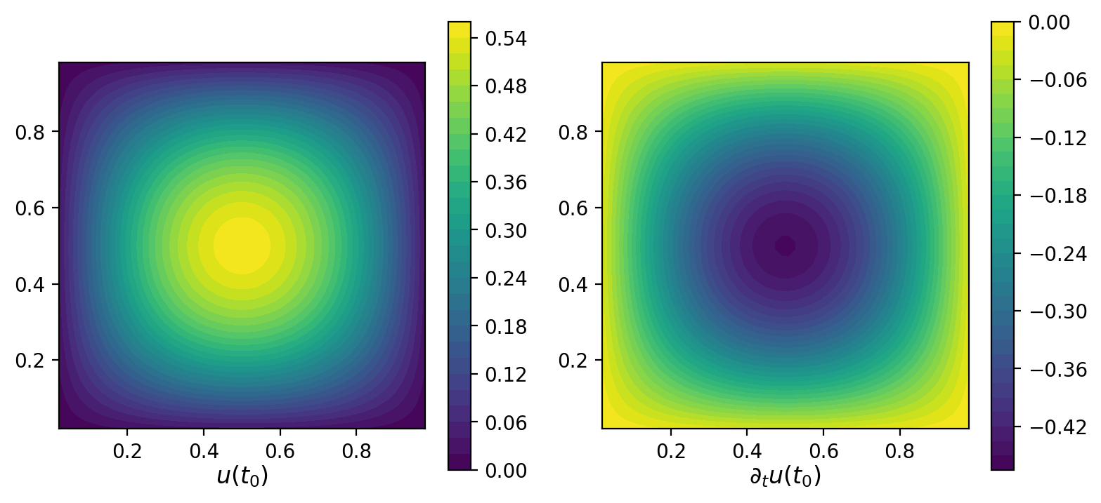
To verify the robustness of the proposed regularization method, we perform numerical tests under four different noise levels: \(\sigma=0\), \(0.001\), \(0.01\) and \(0.1\), respectively. The regularization parameter is fixed at \(\alpha=10^{-5}\) for all test cases. The spatial domain is discretized with a grid of \(2500\) points, and the time step size is set to \(0.005\). The numerical results of the forward problem are illustrated in Figure 1. The inversion results under different noise levels are displayed in Figure 2, and the quantitative evaluation of the reconstruction accuracy is presented in Table 1.

| \(\sigma\) | 0 | 0.001 | 0.01 | 0.1 |
|---|---|---|---|---|
| Error in \(u(t_0)\) | \(2.1262\times 10^{-3}\) | \(2.1366\times 10^{-3}\) | \(3.9080\times 10^{-3}\) | \(3.3806\times 10^{-2}\) |
| Error in \(\partial_t u(t_0)\) | \(7.0512\times 10^{-2}\) | \(7.0628\times 10^{-2}\) | \(7.1672\times 10^{-2}\) | \(8.2700\times 10^{-2}\) |
The results demonstrate the robustness of our proposed algorithm against noise. It can be observed that accurate reconstructions can be obtained even when the noise level is as high as \(0.1\). However, we note that the reconstruction accuracy is highly dependent on the choice of regularization parameters, especially for the velocity component. In particular, the reconstruction accuracy deteriorates significantly when the regularization parameter is set to \(1\times 10^{-3}\) or \(1\times 10^{-5}\) under noise level \(\sigma=0.01\), as detailed in Table 2. This observation further confirms the severe ill-posedness of the backward problem. In the subsequent examples, we will test more high-frequency functions and investigate the effects of the fractional order and the initial time \(t_0\) on the reconstruction errors.
| \(\alpha\) | \(10^{-6}\) | \(10^{-4}\) | \(10^{-3}\) |
|---|---|---|---|
| Error in \(u(t_0)\) | \(3.78\times 10^{-3}\) | \(1.39\times 10^{-2}\) | \(4.06\times 10^{-2}\) |
| Error in \(\partial_t u(t_0)\) | \(8.40\times 10^{-2}\) | \(4.38\times 10^{-1}\) | \(9.15\times 10^{-1}\) |
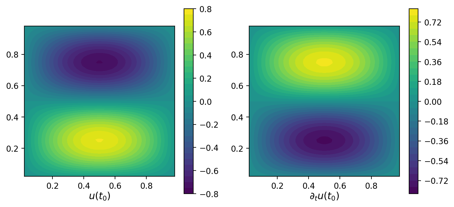
Example 2. In this example, we set \(a=0\) and select the parameter pairs \((\delta,\beta)\) as \((0.2,0.2)\), \((0.4,0.4)\), \((0.6,0.6)\) and \((0.8,0.8)\) to test the impact of the fractional orders. We perform numerical experiments with the following initial displacement condition: \[u_0(x,y)=\sin(2\pi x)\sin(\pi y).\] The noise level is fixed at \(\sigma=0.01\), and we choose \(T=0.5\) and \(t_0=0.4\). All other settings are identical to those in Example 1. The exact solution is presented in Figure 3, and the corresponding reconstructed results are shown in Figure 4. The detailed numerical errors are summarized in Table 3.

| \((\delta,\beta)\) | \((0.2, 0.2)\) | \((0.4, 0.4)\) | \((0.6, 0.6)\) | \((0.8, 0.8)\) |
|---|---|---|---|---|
| Error in \(u(t_0)\) | \(2.7565\times 10^{-3}\) | \(1.5546\times 10^{-3}\) | \(2.4377\times 10^{-3}\) | \(1.8518\times 10^{-2}\) |
| Error in \(\partial_t u(t_0)\) | \(4.1229\times 10^{-2}\) | \(2.3122\times 10^{-2}\) | \(4.0241\times 10^{-2}\) | \(3.6876\times 10^{-1}\) |
The results show that the reconstruction errors increase monotonically as the spatial fractional order increases. This is consistent with the theoretical results in the [21]: as the fractional order becomes larger, the high-frequency components are amplified more significantly, rendering the problem more severely ill-posed. This effect is particularly pronounced for the velocity component. In the following, we present the influence of the initial time \(t_0\) on the reconstruction results to further validate our theoretical analysis.
Example 3. According to the conditional stability analysis, the exponent \(\theta\) of the stability is closely related to the time \(t_0\). As \(t_0\) tends \(0\), the value of \(\theta\) decreases gradually, indicating that the backward problem becomes more severely ill-posed. To verify our theoretical findings, we test the inversion accuracy of our proposed algorithm at different initial times \(t_0\).
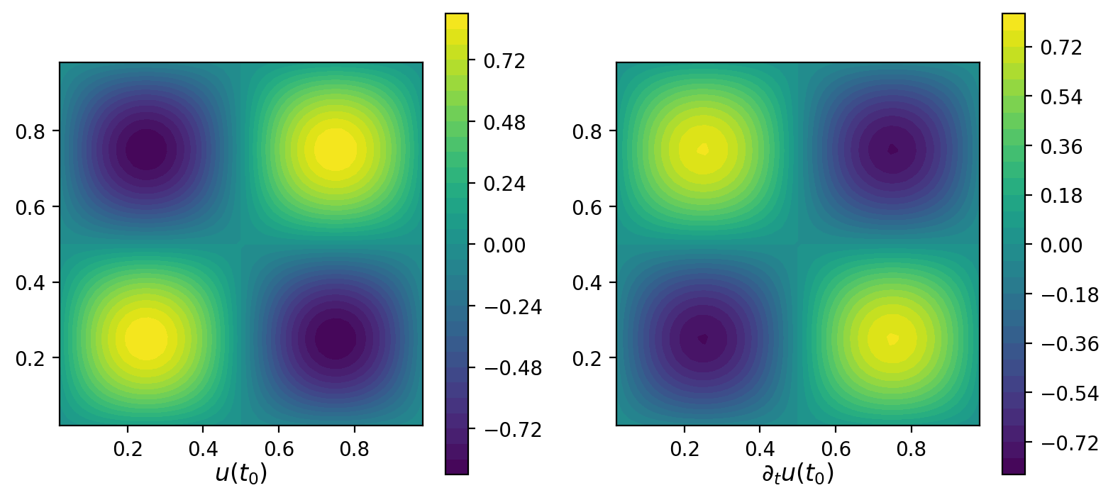
In this numerical experiment, the initial displacement is set as \[u_0(x,y) = \sin(2\pi x)\sin(2\pi y),\] which is a relatively high-frequency function. Compared with the previous two examples, this problem is more challenging. For simplicity, we set \(a=0\) and \(\delta=\beta=0.5\). The noise level is fixed at \(\sigma=0.01\), and all other settings remain consistent with those in Example 1.
To illustrate the exact solution, we present the solution at \(t_0=0.2\) in Figure 5. We perform inversions for \(t_0=0.1, 0.2, 0.3\) and \(0.4\), respectively. The reconstructed results are shown in Figure 6, and the detailed relative errors are summarized in Table 4. To illustrate the dependence of the relative reconstruction errors on the initial time \(t_0\), we present a line plot in Figure 7.

| \(t_0=0.1\) | \(t_0=0.2\) | \(t_0=0.3\) | \(t_0=0.4\) | |
|---|---|---|---|---|
| Error in \(u(t_0)\) | \(3.5845\times 10^{-2}\) | \(1.2523\times 10^{-2}\) | \(6.5248\times 10^{-3}\) | \(6.6968\times 10^{-3}\) |
| Error in \(\partial_t u(t_0)\) | \(6.1160\times 10^{-1}\) | \(1.9312\times 10^{-1}\) | \(3.8288\times 10^{-2}\) | \(9.6682\times 10^{-3}\) |
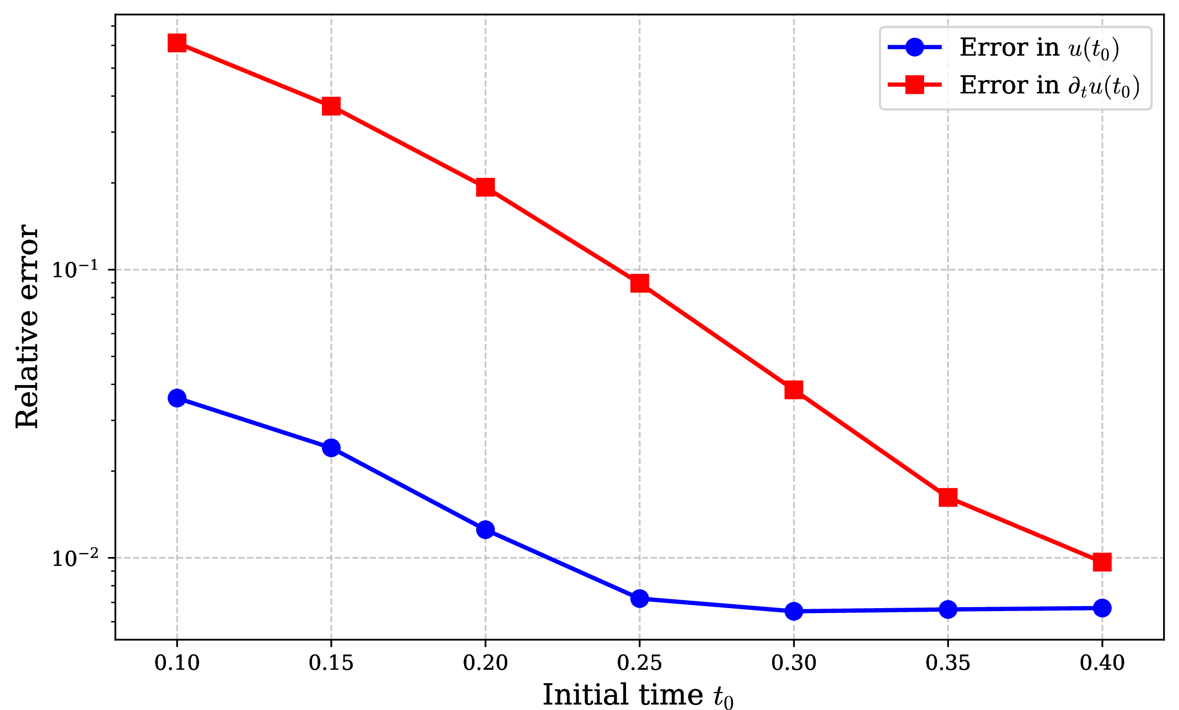
The results demonstrate that as \(t_0\) approaches 0, the reconstruction errors increase significantly, indicating that the problem becomes more severely ill-posed. This is in perfect agreement with our theoretical findings. It can be observed that when \(t_0=0.1\), the reconstruction error for the velocity component is extremely large, leading to a significant deviation from the exact solution.
This behavior is analogous to that of parabolic equations, where it is notoriously difficult to reconstruct solutions near the initial time \(t=0\) from data at the final time \(T\). In contrast, the displacement component can usually be reconstructed with relatively high accuracy. This observation is consistent with the previous two examples, indicating that velocity reconstruction is inherently more challenging. However, a rigorous theoretical explanation for why velocity reconstruction is more difficult than displacement reconstruction is beyond the scope of our current work and will be investigated in our future research.
7 Concluding remarks↩︎
In this work, we established a Carleman estimate for a strongly damped wave equation involving fractional Laplacians \((-\Delta)^\beta\) and \((-\Delta)^\delta\) (\(\delta\le\beta\)). Using the time‑exponential weight \(\varphi(t)=e^{\lambda t}\) and an integral inequality, we proved a conditional stability for the backward problem, with the stability exponent quantifying the ill‑posedness. Based on this stability estimate, we constructed a Tikhonov regularization functional together with the corresponding adjoint system, and derived a convergence rate for the proposed algorithm. Numerical experiments are presented, confirming the effectiveness of the theoretical results.
Future work will extend this framework to equations with time‑fractional damping (e.g., Caputo derivatives). By combining the spatial fractional Carleman estimate developed here with time‑fractional Carleman estimates from [36], we aim to obtain conditional stability and regularization schemes for backward problems involving simultaneous fractional derivatives in both space and time.
References↩︎
Corresponding author 1: lizhiyuan@nbu.edu.cn, supported by the National Natural Science Foundation of China (no. 12271277), Ningbo Youth Leading Talent Project (no. 2024QL045).↩︎