Information Allocation Dynamics in Neural Network Optimization
July 08, 2026
1 Introduction↩︎
An often underestimated fact is that the optimizer is an upstream component in deep learning and affects the whole training process, while the optimizer itself also has implicit bias[[1]][2]. Different first-order optimizers affect not only the speed of loss decrease, but also the training trajectory, the learned representation, and the final generalization behavior[[3]][4]. However, in the standard training paradigm, the optimizer is often treated as a fixed background component. Generalization control relies more on external strategies such as learning-rate scheduling, early stopping, data augmentation, and regularization. A more basic question is therefore often bypassed: how does optimizer implicit bias arise during training, and which training signals does it change?
Existing studies have discussed optimizer implicit bias from several perspectives. SGD[5], Momentum[6], RMSProp[7], Adam[8], and AdamW[9] have different update directions, noise properties, and local geometric preferences. Related work often explains these differences from convergence speed, gradient noise, sharpness, flatness, the Hessian spectrum, or solution-space geometry[10]. These analyses show that the optimizer affects the region finally reached by the model[11]. However, they less directly answer a training-time question: after the same error signal is backpropagated, how does it enter different parameter groups, and how does the optimizer change the actual update ratio of these groups?
This paper starts from the training-time update process and studies an observable form of optimizer implicit bias. In this paper, information allocation refers to the relative update contribution formed by the learning signal across different parameter groups and parameter components. In other words, we do not focus on where the model finally stops. We focus on which parameter pathways more easily write in the current error signal during training, which pathways are relatively weakened, and how this difference further changes later gradient statistics.
This issue is especially clear in adaptive optimizers. Adam-like methods maintain first-moment and second-moment estimates and use the exponential moving average of the second moment to construct coordinate-wise update gains. The standard interpretation treats this process as adaptive preconditioning or coordinate-wise rescaling. This paper further points out that when different coordinates have different second-moment statistics, preconditioning changes not only the update magnitude of each coordinate but also the relative update ratio between parameter groups. Therefore, adaptive preconditioning has not only numerical scaling meaning but also training-time allocation meaning. This is one source of optimizer implicit bias.
To characterize this effect, this paper uses a continuous preconditioning exponent \(p\) as an analysis interface[12]. In a unified form, the update can be written as a first-order direction multiplied by a gain from the second-moment channel, where \(p\) controls the degree to which the second moment enters the update. When \(p=0\), the update is close to an SGDM-like form, and the second moment does not explicitly change coordinate ratios. When \(p=1/2\), the update is close to an Adam-like form. Intermediate values correspond to different strengths of diagonal preconditioning.
The roles of \(p\) and the learning rate are different. With fixed gradients and fixed optimizer states, the learning rate mainly scales all parameter updates by the same factor. In contrast, \(p\) changes the relative gain of different coordinates through the second-moment estimate, so it can directly change the relative update between parameter groups. For nonlinear deep networks, a larger learning rate can also indirectly affect later update ratios by changing the next parameter position, residual structure, and gradient statistics. However, this effect comes from trajectory feedback, not from the learning rate directly changing the relative preconditioning gain in the current step.
This paper uses weight and bias as the minimal analysis objects. They often appear in the same linear or convolutional layer and act on the same output error, but they receive the error signal in different ways. The weight gradient depends on the correlation between input activations and errors, so it more directly corresponds to the correction of input-dependent structure. The bias gradient mainly depends on the aggregation of errors over the batch or spatial dimensions, so it more directly corresponds to output shift and local calibration. Thus, the same error signal does not enter weight and bias in the same way. Once the optimizer applies different effective gains to them, it changes the relative update contribution of the two parameter types to the current error.
Based on this analysis, this paper approximately divides parameters in modern networks into weight-like pathways and bias-like pathways. The weight-like pathway includes weights in linear layers, convolutional layers, attention projections, and FFNs. The bias-like pathway includes explicit biases and normalization affine parameters. This grouping does not mean that all bias-like parameters have exactly the same mathematical role. It is used to keep a consistent observation protocol across different network architectures. By recording gradient norms, update norms, second-moment statistics, and relative update ratios of the two groups, we can directly observe how different values of \(p\) affect the training process.
The experiments are designed around this point. First, in a controlled single-layer path-allocation experiment, we directly measure the contribution ratio from the weight pathway and the bias pathway in the output change. Second, on constructed datasets and classical vision tasks, we observe how fixed \(p\) and dynamic \(p\) change the loss curve, accuracy curve, update ratio, and sample fitting order. Finally, in partially pretrained settings, we further examine whether this regulation affects the update state between the pretrained backbone and the task-specific head. The focus of this paper is not a single best accuracy value. Instead, we study how different preconditioning strengths change the parameter update structure during training.
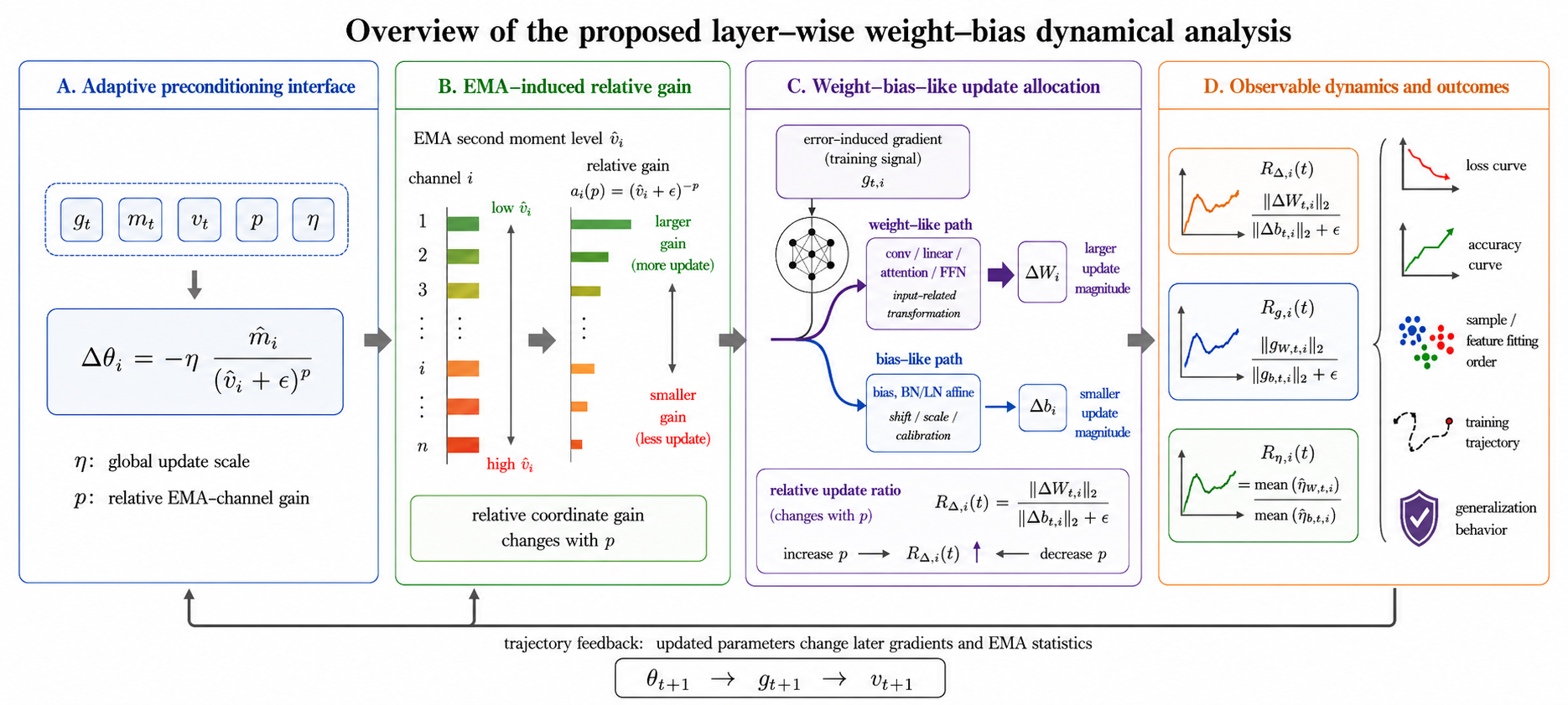
The main contributions of this paper are as follows.
First, this paper proposes weight–bias relative update dynamics as a training-time phenomenon. We show that adaptive preconditioning changes not only coordinate-wise update magnitude, but also the relative write-in ratio of training signals between weight-like and bias-like parameter pathways. This phenomenon provides an observable training-time entry point for understanding optimizer implicit bias.
Second, this paper derives the different gradient sources of weight and bias for the same residual signal in a minimal linear model, and explains how preconditioned updates change the relative strength between the input-dependent correction term and the mean-calibration correction term. This analysis gives a minimal mechanism for weight–bias relative update dynamics.
Third, this paper verifies the above mechanism through controlled experiments and real deep-network experiments. The results show that different preconditioning strengths systematically change the weight/bias-like update ratio and further affect the optimization path, loss curve, accuracy curve, and generalization behavior.
Fourth, this paper reinterprets the role of the partially adaptive exponent \(p\) from the perspective of weight–bias relative update dynamics. The results show that a smaller \(p\) does not necessarily lead to better generalization. Different tasks and training stages may require different update ratios across parameter pathways. Therefore, \(p\) is better understood as an interface for regulating the training-time update structure, rather than as a one-directional parameter for improving generalization.
2 Related Work↩︎
This section reviews several lines of work related to this paper. We first introduce first-order optimizers and adaptive preconditioning, because the continuous exponent \(p\) used in this paper is built on the Adam-like second-moment preconditioning term. We then discuss partial adaptivity, optimizer implicit bias, parameter grouping and layer-wise training diagnostics, and training-control strategies. These studies show the importance of optimizer update rules, preconditioning strength, parameter-type differences, and dynamic scheduling. They also provide background for the later analysis of weight–bias relative update dynamics.
2.1 First-order Optimizers and Adaptive Preconditioning↩︎
First-order optimizers use the mini-batch gradient \[g_t=\nabla_{\theta}\mathcal{L}_t(\theta_t) \label{eq:rw95gradient}\tag{1}\] as the main source of information and minimize the training objective through iterative updates. SGD, Momentum, RMSProp, Adam, and AdamW differ in their specific forms. From a unified view, however, they can all be written as updates determined jointly by a first-order direction and a preconditioning factor: \[\theta_{t+1} = \theta_t - \eta_t P_t \tilde{g}_t, \label{eq:rw95unified95first95order}\tag{2}\] where \(\eta_t\) is the learning rate, \(\tilde{g}_t\) denotes a first-order direction that may be smoothed by momentum, and \(P_t\) is a preconditioning factor determined by the optimizer state. If \(P_t=I\) or is approximately constant, the update is close to SGD or Momentum. If \(P_t\) changes coordinate-wise with historical gradient statistics, the update becomes an adaptive method such as RMSProp, Adam, or AdamW.
The core of Adam-like methods is to maintain both first-moment and second-moment estimates: \[m_t = \beta_1m_{t-1} + (1-\beta_1)g_t, \qquad v_t = \beta_2v_{t-1} + (1-\beta_2)g_t^2. \label{eq:rw95adam95m95v}\tag{3}\] After bias correction, Adam uses \(\hat{m}_t/(\sqrt{\hat{v}_t}+\epsilon)\) to construct a coordinate-wise update direction. AdamW further shows that conventional \(L_2\) regularization and weight decay are no longer equivalent in adaptive optimizers, and therefore decouples weight decay from the gradient update. These methods show that modern optimizers do not simply move along the gradient direction. They change the effective update magnitude of different coordinates according to historical gradient statistics.
2.2 Partial Adaptivity and the Preconditioning Exponent↩︎
In Adam-like methods, the second moment usually enters the denominator in square-root form. More generally, a continuous exponent can be used to control the strength of second-moment preconditioning: \[\Delta\theta_{t,i} = - \eta_t \frac{\hat{m}_{t,i}}{(\hat{v}_{t,i}+\epsilon)^p}, \label{eq:rw95p95update}\tag{4}\] where \(i\) denotes a parameter coordinate and \(p\) controls how strongly the second-moment estimate enters the update. When \(p=0\), the update does not explicitly depend on \(\hat{v}_t\) and is formally close to a momentum-like update. When \(p=1/2\), the update is close to an Adam-like update. Methods such as Padam have shown that continuously changing this exponent can form intermediate states between SGD-like and Adam-like updates and can try to reduce the generalization gap between adaptive and non-adaptive optimizers.
Existing partially adaptive methods mainly treat \(p\) as a hyperparameter for adaptivity strength. A larger \(p\) means stronger second-moment normalization, while a smaller \(p\) means weaker adaptive preconditioning. This view is important for comparing SGD-like and Adam-like methods, and it also suggests the potential to integrate different optimization theories under a common framework.
2.3 Optimizer Implicit Bias and Generalization Differences↩︎
Many studies show that optimizers are not neutral numerical tools. Different optimizers can produce different training trajectories, reachable solutions, and generalization behavior even when they optimize the same loss function. In deep networks, Adam-like methods often have faster early loss decrease and better numerical stability, while SGD or Momentum often show different final generalization behavior in some vision tasks. These phenomena have been explained from optimization trajectories, gradient noise, sharpness/flatness, curvature structure, and implicit regularization.
This line of work shows that the optimizer affects where the model finally stays, and also affects how the model explores parameter space during training. For example, learning rate, batch size, momentum, and adaptive preconditioning all change the randomness and directionality of the training trajectory. Accordingly, optimizer implicit bias is usually described as a preference over the final solution space or function space.
2.4 Parameter Groups, Bias Treatment, and Layer-wise Training Diagnostics↩︎
Modern deep-learning practice has already noticed differences between parameter types. A typical example is parameter grouping for weight decay. In early training recipes, weight decay was sometimes applied to all learnable parameters, including convolution kernels, linear weights, biases, and normalization parameters. Later, many training recipes adopted no bias decay or no decay for normalization parameters. That is, weight decay is applied only to weights in convolutional and fully connected layers, but not to biases, BatchNorm \(\gamma,\beta\), or other one-dimensional calibration parameters.
This practice shows that existing training pipelines do not treat all parameters as fully equivalent. Convolution kernels and linear weights usually perform input-dependent feature transformations and directly determine mappings across channels, spatial positions, or tokens. Biases and normalization affine parameters are more involved in shifts, scale calibration, or local output adjustment. They play different roles in networks and are therefore often treated differently in regularization and optimizer parameter groups. After AdamW decouples weight decay from the adaptive gradient update, this parameter grouping becomes more common, because decay, learning rate, and adaptive update can be specified more clearly.
However, existing parameter-group methods are mostly used as implementation details, regularization strategies, or training heuristics. For example, no weight decay for bias is usually viewed as an empirical strategy to avoid over-regularization. No decay for normalization parameters is usually viewed as a training recipe for preserving scale and shift calibration. These practices show that the differences between weight, bias, and normalization parameters have been noticed, but they usually do not further explain why these parameter types obtain different gradient statistics in adaptive optimizers, how second-moment preconditioning changes their relative updates, or how this relative update change affects the training trajectory.
Layer-wise gradient-norm and parameter-norm diagnostics are also widely used for training monitoring. Researchers and practitioners often record the gradient norm, update norm, or weight norm of each layer to check gradient explosion, gradient vanishing, differences in layer-wise learning speed, and numerical stability. Similarly, layer-wise learning rates, layer-wise adaptive rate scaling, and parameter-group learning rates show that different layers and different parameter groups can use different update scales.
2.5 Training Control and Dynamic Optimization Strategies↩︎
Besides the optimizer itself, scheduling strategies during training also strongly affect the final model. Learning-rate warmup, step decay, cosine annealing, cyclic learning rates, early stopping, and optimizer switching are common training-control methods. These methods usually do not change the loss function. Instead, they change the update scale, exploration range, or convergence pace during training.
Learning-rate scheduling mainly controls the global step size. With fixed gradients and fixed optimizer states, the learning rate scales all parameter updates up or down by the same factor. Therefore, it does not directly change the update ratio between different parameter groups within the same step. However, in multi-step training of nonlinear networks, a larger learning rate can move parameters to different positions and change later gradients through curvature coupling, residual changes, and EMA feedback. Thus, the learning rate is not a direct relative-allocation parameter, but it can indirectly affect later parameter-group dynamics through trajectory feedback.
Optimizer switching changes the update rule in a discrete way. For example, one may use AdamW in the early training stage for fast and stable decrease, and then switch to SGD in the later stage for different convergence behavior. These strategies suggest that different training stages may need different update preferences. However, optimizer switching is usually coarse-grained. It directly replaces the whole update rule instead of continuously regulating the relative gain inside adaptive preconditioning.
2.6 Summary↩︎
In summary, existing work has shown from several perspectives that the optimizer affects the training process and final generalization. Studies on first-order optimizers and adaptive preconditioning provide the basic form of update rules. Partially adaptive methods show that the strength of second-moment preconditioning can be continuously adjusted. Studies on implicit bias show that different optimizers lead to different training trajectories and solution preferences. Parameter grouping and training recipes such as no bias decay show that weight, bias, and normalization parameters are not fully equivalent in practice. Learning-rate scheduling and optimizer switching further show that different training stages may require different update states.
However, these directions are usually discussed separately. Existing work rarely puts the gradients, updates, and second-moment statistics of layer-wise weight and bias-like parameters into the same dynamical framework. It also rarely discusses how the continuous preconditioning exponent \(p\) changes their relative update ratio. The following sections start from this perspective. We treat \(p\) as an interface for observing the state of adaptive preconditioning, and analyze the effect of the optimizer on training through weight–bias relative update statistics.
3 Weight–Bias Information Allocation↩︎
Existing analyses of adaptive optimizers mostly focus on normalized coordinate-wise scaling within a layer. Adam-like methods change the effective step size of different coordinates through first-moment and second-moment estimates, and are therefore often understood as coordinate-wise preconditioning mechanisms. However, different parameter forms in neural networks correspond to different differential pathways. They write the same training signal into different parts of the network in different ways and with different strengths. Analyzing optimizers only from coordinate-wise scaling can miss the information-allocation difference caused by parameter form.
This section discusses two classical parameter pathways: weight and bias. They often appear in the same output unit, but their differential forms with respect to the residual are different. The weight gradient preserves input correlation and mainly corresponds to corrections of input structure. The bias gradient preserves the residual mean direction and mainly corresponds to output shift and local calibration. Therefore, the optimizer not only changes the update size of each coordinate. It may also change the write-in ratio of the training signal between the input-dependent pathway and the bias pathway.
We first define information allocation and use a minimal linear model to decompose the gradient sources of weight and bias. We then introduce a continuous exponent \(p\) and show how it changes coordinate-wise gain through EMA preconditioning, and further changes the relative update between weight and bias. Finally, this section extends the decomposition to bias-like parameters in modern networks and constructs a simple \(p\) control rule based on gradient statistics of weight and bias-like parameter groups. This rule does not assume that one fixed \(p\) is always optimal. It checks whether gradient statistics can provide feedback for stage-wise adjustment of \(p\).
3.1 Information Allocation↩︎
Let the current parameter be \(\theta_t\), and let the current mini-batch loss be \(\mathcal{L}_t(\theta_t)\). The gradient is \[g_t = \nabla_{\theta}\mathcal{L}_t(\theta_t). \label{eq:mini95batch95gradient}\tag{5}\] The optimizer uses the gradient and its internal state to generate an update: \[\theta_{t+1} = \theta_t+\Delta\theta_t, \qquad \Delta\theta_t = -\eta_t\mathcal{P}_t(g_t;s_t), \label{eq:gradient95to95update95operator}\tag{6}\] where \(\eta_t\) is the learning rate, and \(\mathcal{P}_t(\cdot)\) denotes the gradient transformation given by the optimizer. For SGD, \(\mathcal{P}_t(\cdot)\) is mainly determined by the gradient or momentum. For Adam-like methods, \(\mathcal{P}_t(\cdot)\) also depends on the first-moment and second-moment estimates.
The distinction between gradient and update is central to this study. The gradient \(g_t\) describes the local sensitivity of the loss to the parameters. It can be viewed as the model’s demand for an expected update. The update \(\Delta\theta_t\) describes the signal that the optimizer actually writes into the model.
Given a parameter partition \(\{G_1,\ldots,G_K\}\), the update can be written as \[\Delta\theta_t = \left( \Delta\theta_{G_1,t}, \Delta\theta_{G_2,t}, \ldots, \Delta\theta_{G_K,t} \right). \label{eq:allocation95decomposition}\tag{7}\] Here \(\Delta\theta_{G_k,t}\) is the actual update of parameter group \(G_k\). Different optimizers change the relative magnitude of these update components. When the signal actually written by the optimizer changes, the order and strength with which the training signal enters different parameter pathways also change, and this further affects later gradients.
3.2 Minimal Model: Gradient Sources of Weight and Bias↩︎
Weight and bias form a minimal and common pair of analysis objects. In linear and convolutional layers, weights perform input-dependent transformations, while biases perform output shifts. This division appears in the simplest linear model and can also extend to deeper network structures.
Consider the following single-channel linear output: \[z = Xw+b\mathbf{1}, \label{eq:minimal95linear95model}\tag{8}\] where \(X\in\mathbb{R}^{n\times d}\) is the input matrix, \(w\in\mathbb{R}^{d}\) is the weight, \(b\in\mathbb{R}\) is the bias, and \(\mathbf{1}\in\mathbb{R}^{n}\) is the all-one vector. Let the target be \(y\in\mathbb{R}^{n}\), and define the residual as \[r = z-y = Xw+b\mathbf{1}-y. \label{eq:minimal95residual}\tag{9}\] We use the squared loss \[\mathcal{L} = \frac{1}{2n}\|r\|_2^2. \label{eq:minimal95loss}\tag{10}\] The gradients of weight and bias are \[g_w = \nabla_w\mathcal{L} = \frac{1}{n}X^\top r, \qquad g_b = \nabla_b\mathcal{L} = \frac{1}{n}\mathbf{1}^\top r. \label{eq:minimal95gradients}\tag{11}\] Here \(X^\top r\) projects the residual onto input-dependent directions. As long as part of the residual is correlated with input structure, it enters the weight gradient. In contrast, \(\mathbf{1}^\top r\) preserves only the component of the residual in the constant direction, namely the residual mean.
Let \[\bar r = \frac{1}{n}\mathbf{1}^\top r. \label{eq:residual95mean}\tag{12}\] Then the bias gradient is \(g_b=\bar r\). The corresponding mean projection is \[\frac{1}{n}\mathbf{1}\mathbf{1}^\top r = \bar r\mathbf{1}. \label{eq:bias95mean95projection}\tag{13}\] This shows that the bias directly corrects the mean direction of the residual. It does not distinguish different input features, but provides a shift correction to the whole output channel.
Now consider one preconditioned update: \[\Delta w = -\eta Q_w g_w, \qquad \Delta b = -\eta q_b g_b, \label{eq:preconditioned95weight95bias95update}\tag{14}\] where \(Q_w\) is the diagonal preconditioning matrix for the weight, and \(q_b\) is the scalar preconditioning factor for the bias. The residual after the update is \[\begin{align} r^+ &= X(w+\Delta w)+(b+\Delta b)\mathbf{1}-y \notag\\ &= r+X\Delta w+\Delta b\,\mathbf{1}. \label{eq:residual95after95update95a} \end{align}\tag{15}\] Substituting Eq. 11 and Eq. 14 gives \[r^+ = r - \frac{\eta}{n}XQ_wX^\top r - \frac{\eta}{n}q_b\mathbf{1}\mathbf{1}^\top r. \label{eq:residual95after95update}\tag{16}\] The first term corrects input-dependent residuals, and the second term corrects the residual mean. The optimizer changes the relative strength of these two correction terms through \(Q_w\) and \(q_b\). Thus, weight–bias information allocation can be understood as the difference in how the same residual signal is allocated between input-dependent correction and mean correction.
This model is small, but it is sufficient to show the key point. The difference between weight and bias lies in how they project the residual signal. The later regulation by \(p\) acts on the preconditioning matrix and therefore changes the relative ratio of these two residual corrections.
3.3 The \(p\) Interface: From Coordinate-wise Gain to Weight–Bias Allocation↩︎
Adam-like methods use first-moment and second-moment estimates to construct updates. Let \[m_t = \beta_1m_{t-1}+(1-\beta_1)g_t, \qquad v_t = \beta_2v_{t-1}+(1-\beta_2)g_t^2. \label{eq:ema95m95v}\tag{17}\] After bias correction, they are denoted by \(\hat{m}_t\) and \(\hat{v}_t\). This paper writes the update with a continuous exponent \(p\) as \[\Delta\theta_{t,i} = -\eta_t \frac{\hat{m}_{t,i}}{(\hat{v}_{t,i}+\epsilon)^p}, \label{eq:p95update}\tag{18}\] where \(i\) is a parameter coordinate. Define the coordinate-wise gain as \[a_{t,i}(p) = (\hat{v}_{t,i}+\epsilon)^{-p}. \label{eq:p95gain}\tag{19}\] The update can then be written as \[\Delta\theta_{t,i} = -\eta_t a_{t,i}(p)\hat{m}_{t,i}. \label{eq:p95update95gain95form}\tag{20}\] Here \(p\) controls how strongly the second moment enters the update. When \(p=0\), the second moment does not participate in scaling, and the update reduces to a momentum-like form: \[\Delta\theta_{t,i} = -\eta_t\hat{m}_{t,i}. \label{eq:p95zero95update}\tag{21}\] When \(p=1/2\), the update corresponds to an Adam-like form: \[\Delta\theta_{t,i} = -\eta_t \frac{\hat{m}_{t,i}}{(\hat{v}_{t,i}+\epsilon)^{1/2}}. \label{eq:p95half95update}\tag{22}\]
For two coordinates \(i\) and \(j\), after ignoring \(\epsilon\), the update-magnitude ratio is approximately \[\frac{|\Delta\theta_{t,i}|}{|\Delta\theta_{t,j}|} \approx \frac{|\hat{m}_{t,i}|}{|\hat{m}_{t,j}|} \left( \frac{\hat{v}_{t,j}}{\hat{v}_{t,i}} \right)^p. \label{eq:p95ratio}\tag{23}\] Here \(p\) changes the relative update ratio between coordinates. The learning rate \(\eta_t\) changes the global step size, while \(p\) changes the coordinate-wise gain defined by the second moment. This difference is important in later experiments, because changing the learning rate and changing \(p\) do not produce the same weight–bias allocation.
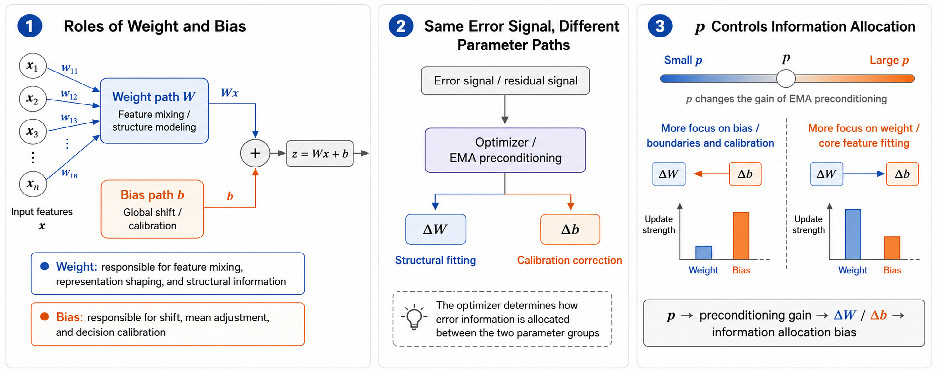
Writing Eq. 18 back into the minimal model gives \[\Delta w = -\eta Q_w(p)g_w, \qquad \Delta b = -\eta q_b(p)g_b, \label{eq:p95weight95bias95update}\tag{24}\] where \[Q_w(p) = \operatorname{diag}\left((\hat{v}_w+\epsilon)^{-p}\right), \qquad q_b(p) = (\hat{v}_b+\epsilon)^{-p}. \label{eq:p95weight95bias95preconditioner}\tag{25}\] Therefore, \[r^+ = r - \frac{\eta}{n}XQ_w(p)X^\top r - \frac{\eta}{n}q_b(p)\mathbf{1}\mathbf{1}^\top r. \label{eq:p95residual95after95update}\tag{26}\] Here \(Q_w(p)\) and \(q_b(p)\) determine the relative strength of the weight correction term and the bias correction term. A fixed \(p\) gives a fixed preconditioning geometry. A dynamic \(p\) allows the training process to change this geometry at different stages.
3.4 Information Allocation Control Under Sparse Inputs↩︎
The previous subsection gives the general form of \(p\). Under sparse inputs, this mechanism has a more intuitive explanation. Consider the \(j\)-th coordinate of the weight. From Eq. 11 , \[g_{w,j} = \frac{1}{n}\sum_{i=1}^{n}x_{ij}r_i. \label{eq:coordinate95weight95gradient}\tag{27}\] If the input coordinate \(x_{ij}\) is zero most of the time, then the gradient of this coordinate is also sparser. Suppose that the probability that the \(j\)-th input coordinate is nonzero in a mini-batch is approximately \(\pi_j\), and that the average magnitude of the squared gradient when it is nonzero is \(\sigma_j^2\). In a stable stage, the expected scale of the second-moment EMA can be approximated as \[\mathbb{E}[v_{w,j}] \approx \pi_j\sigma_j^2. \label{eq:sparse95v95expectation}\tag{28}\] The corresponding coordinate-wise gain is \[a_j(p) = (\hat{v}_{w,j}+\epsilon)^{-p} \approx (\pi_j\sigma_j^2+ \epsilon)^{-p}. \label{eq:sparse95coordinate95gain}\tag{29}\] When \(\epsilon\) is not dominant, \[a_j(p) \propto \pi_j^{-p}. \label{eq:sparse95gain95pi}\tag{30}\]
This approximation shows that low-frequency or sparse coordinates have smaller second moments, and a larger \(p\) amplifies their relative gains. In other words, \(p\) changes the update ratio between low-frequency and high-frequency coordinates. This ratio change cannot be reproduced by simple learning-rate scaling, because the learning rate multiplies all coordinates at the same time, while \(p\) changes the relative weights of different coordinates through \(\hat{v}\).
In the weight–bias case, this phenomenon affects how the two parameter types obtain updates. If some weight coordinates are activated only by a small number of samples or local features, their \(\hat{v}\) may be small. A larger \(p\) increases the relative update of these coordinates. If the second moment of bias or bias-like parameters changes more smoothly, the relative update ratio between the two groups also changes with \(p\). Therefore, \(p\) can be viewed as an interface for controlling information allocation. It does not directly specify which parameter is important. It changes the effective gains of different coordinates and parameter groups through EMA statistics.
Therefore, under the sparse-input condition above, a larger \(p\) tends to increase the relative write-in of low-second-moment weight coordinates, so more residual signal enters the model through the input-dependent pathway. A smaller \(p\) weakens this coordinate selectivity and allows the bias-like calibration pathway to occupy a higher proportion in the relative update. Here \(p\) changes the effective gains of different coordinates and parameter groups through EMA statistics, and thus regulates weight–bias information allocation.
It should be noted that \(p\) may not be the only effective control variable. This paper uses \(p\) as the interface mainly because it unifies the EMA-statistics form.
3.5 Parameter Grouping in Modern Networks↩︎
The minimal model above contains only one weight and one bias, so it can clearly decompose input-dependent correction and bias correction. Real networks have more complex parameter forms. The same module may contain linear transformations, convolutional transformations, normalization parameters, and shift parameters. For each modern network module, we introduce the core distinction from the minimal model: whether the training signal is mainly written into the model through an input-dependent transformation, or through a bias and calibration pathway.
Based on this principle, this paper approximately divides parameters in modern networks into two groups. The first group is weight parameters. They usually participate in input-dependent transformations and determine mappings between features, channels, or tokens. The second group is bias-like parameters. They usually participate in output shifts, post-normalization shift calibration, or local scale calibration. Table 1 summarizes the parameter-grouping rule used in this paper.
| Module | Parameter type | Main role | Group in this paper |
|---|---|---|---|
| Linear / Fully-connected | weight | Input-dependent linear transformation | weight |
| Linear / Fully-connected | bias | Output shift | bias-like |
| Convolution | weight | Local spatial and channel transformation | weight |
| Convolution | bias | Output-channel shift | bias-like |
| BatchNorm | scale \(\gamma\) | Channel scale calibration | bias-like |
| BatchNorm | shift \(\beta\) | Channel shift calibration | bias-like |
| LayerNorm | scale \(\gamma\) | Feature scale calibration | bias-like |
| LayerNorm | shift \(\beta\) | Feature shift calibration | bias-like |
| Attention projection | weight | Token or channel transformation | weight |
| Attention projection | bias | Projection-output shift | bias-like |
| FFN / MLP block | weight | Nonlinear feature transformation | weight |
| FFN / MLP block | bias | Hidden or output shift | bias-like |
The later experiments mainly record gradient statistics and update statistics of the weight parameter group and the bias-like parameter group. The weight group includes weights in linear layers, convolutional layers, attention projections, and FFNs. The bias-like group includes explicit biases and normalization affine parameters. It should be noted that a normalization scale parameter is not the same as an additive bias, but it participates in local scale calibration. Therefore, this paper includes it in the broad bias-like parameter group. This treatment is not intended to build a strict two-class theory for all modules. It is used to keep a consistent observation protocol across different network architectures.
3.6 Weight–Bias Gradient Statistics↩︎
The minimal model gives two gradient sources: \(X^\top r\) and \(\mathbf{1}^\top r\). In deep networks, a single residual \(r\) is no longer easy to decompose directly, but the gradients of weight and bias-like parameter groups can still be measured. This paper uses these gradient statistics to observe the training signal currently received by the two parameter groups.
Assume that epoch \(e\) contains \(T_e\) iterations. Define the average gradient norms of the weight group and the bias-like group as \[D_w(e) = \frac{1}{T_e} \sum_{t\in e} \|g_{w,t}\|_2, \qquad D_b(e) = \frac{1}{T_e} \sum_{t\in e} \|g_{b,t}\|_2. \label{eq:weight95bias95gradient95statistics}\tag{31}\] Here \(g_{w,t}\) is the gradient of the weight parameter group at step \(t\), and \(g_{b,t}\) is the gradient of the bias-like parameter group.
These statistics describe the gradient strength of the two parameter groups in the current training stage. According to the minimal model, a larger \(D_w(e)\) usually means that input-dependent transformations still have strong training signals, while a larger \(D_b(e)\) means that calibration-related parameters still have strong training signals. Therefore, \(D_w(e)\) and \(D_b(e)\) can be used as feedback variables for adjusting \(p\).
To observe stage-wise changes, define the relative change rates as \[\delta_w(e) = \frac{D_w(e)-D_w(e-1)}{D_w(e-1)+\epsilon}, \qquad \delta_b(e) = \frac{D_b(e)-D_b(e-1)}{D_b(e-1)+\epsilon}. \label{eq:weight95bias95gradient95change}\tag{32}\] Here \(\delta_w(e)\) and \(\delta_b(e)\) record the changing trends of the two gradient statistics.
In practical training, the statistics of a single epoch may fluctuate. To avoid continuing to increase \(p\) after the gradient of bias-like parameters rebounds from a low level, we record \[D_b^{\min}(e) = \min_{s\le e}D_b(s). \label{eq:bias95gradient95min}\tag{33}\] If \(D_b(e)\) is clearly higher than this historical low value, then the training signal of calibration-related parameters has strengthened again. This signal is used in the control rule below.
3.7 Gradient-statistics-based \(p\) Control↩︎
This subsection gives a simple \(p\) control rule. The algorithm keeps \(p\) fixed within one epoch. At the end of the epoch, it computes \(D_w(e)\), \(D_b(e)\), \(\delta_w(e)\), and \(\delta_b(e)\), and then updates the \(p\) used in the next epoch.
The basic form is \[p_{e+1} = \operatorname{clip} \left( p_e+\Delta p_e, p_{\min}, p_{\max} \right), \label{eq:p95control95general}\tag{34}\] where \(p_e\) is the exponent used in epoch \(e\), \(\Delta p_e\) is the adjustment, and \([p_{\min},p_{\max}]\) is the allowed range.
The control rule is conservative. If the gradient statistics of bias-like parameters rebound clearly, the algorithm decreases \(p\) to avoid making the update overly biased toward coordinates selected by the second moment. If the gradient statistics of bias-like parameters decrease and the weight gradient statistics do not increase at the same time, the algorithm increases \(p\) to strengthen coordinate selectivity. If the two gradient statistics increase at the same time, the algorithm keeps \(p\) unchanged to avoid changing the preconditioning geometry when the overall training pressure increases.
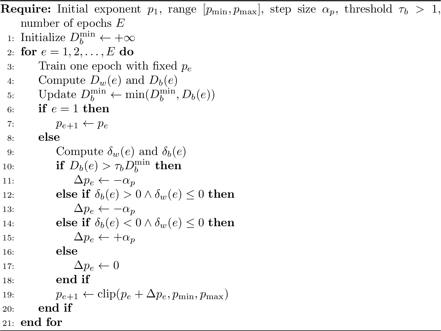
This algorithm uses gradient statistics as feedback and treats \(p\) as the control variable. The relation can be written as \[\text{gradient statistics} \longrightarrow p\text{-update} \longrightarrow \text{weight--bias information allocation}. \label{eq:statistics95control95loop}\tag{35}\] This is only a basic implementation. More complex smoothing, thresholds, and grouping strategies can be compared in the experiments. The main point here is that the adjustment of \(p\) is based on the training state of the weight and bias-like parameter groups, rather than on a pre-defined fixed schedule for the whole training process.
3.8 Testable Predictions↩︎
The analysis above gives several direct experimental predictions.
First, a fixed \(p\) should change the relative update between weight and bias-like parameters. If \(p\) only changes the global step size, then after matching the update scale, the weight/bias update ratio under different values of \(p\) should not show systematic differences. If \(p\) changes the preconditioning geometry, this ratio should vary with \(p\).
Second, low-frequency or sparse coordinates should be more sensitive to \(p\). Since \(a_j(p)\propto \pi_j^{-p}\), when some coordinates have a low activation probability, a larger \(p\) amplifies their relative gains. Therefore, different values of \(p\) may change the fitting order of low-frequency features, boundary samples, or sparse activation regions.
Third, the gradient statistics of weight and bias-like parameters do not have to change synchronously. If they correspond to input-dependent transformations and local calibration, respectively, different gradient trends may appear at different training stages. This provides observable feedback for dynamic \(p\).
Fourth, gradient-statistics-based \(p\) control should produce training trajectories different from fixed \(p\), hand-designed schedules, and learning-rate schedules. If the information allocation mechanism holds, dynamic \(p\) should change not only the loss curve, but also the weight/bias update ratio, the gradient statistics of bias-like parameters, and the timing of validation performance or overfitting.
Fifth, bias-like parameters should show related trends in modern networks. Explicit biases, normalization shifts, and some scale parameters all participate in local calibration. If weight–bias information allocation holds, changes in \(p\) should affect the update timing of these parameters.
This section gives the basic analysis of weight–bias information allocation. The core conclusion is that \(p\) changes not only update magnitude, but also the relative updates obtained by weight and bias-like parameters. The next section verifies this mechanism with fixed \(p\), dynamic \(p\), and gradient-statistics-based \(p\) control.
4 Experiments and Discussion↩︎
4.1 Optimization Dynamics and Sample-level Information Allocation↩︎
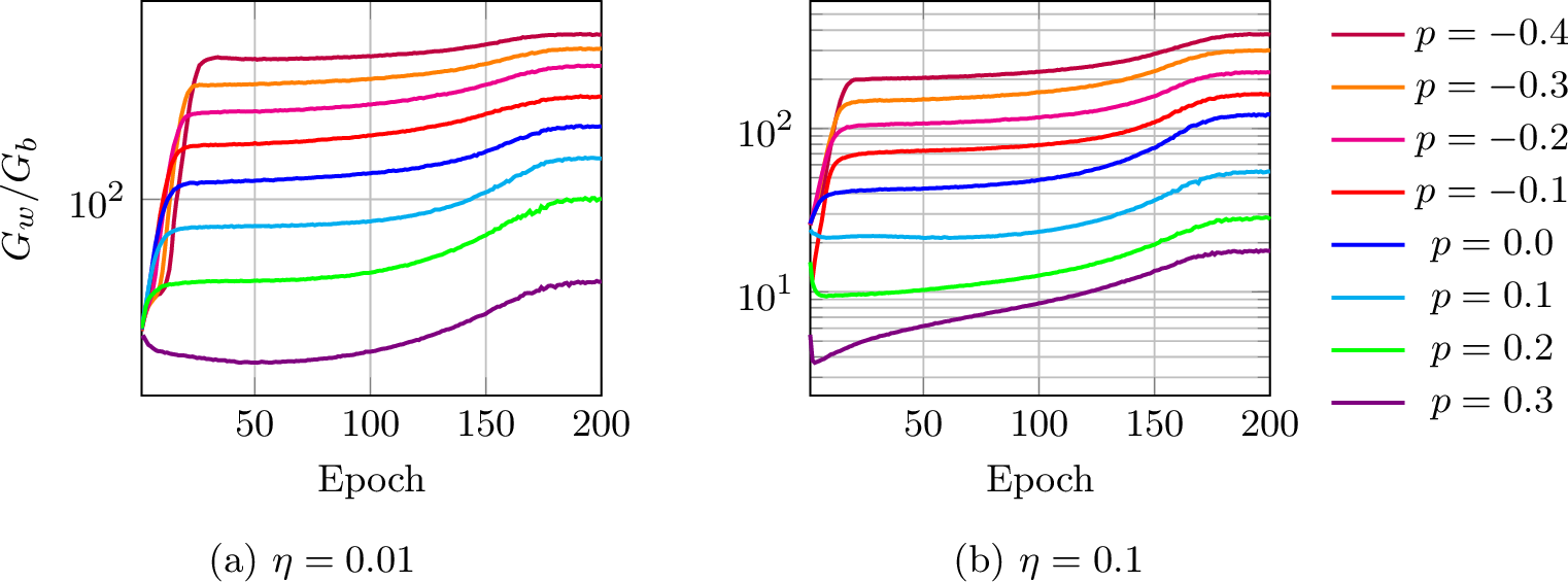
To examine whether the allocation exponent \(p\) only changes final accuracy or systematically changes training dynamics, this paper records parameter-group statistics and sample-level loss trajectories during training. Specifically, we track both global and layer-wise weight-to-bias gradient norm ratios, denoted by \(G_w/G_b\), and record the loss distributions of clean train and test samples under each fixed value of \(p\). In addition, we save per-sample losses at every epoch. This allows us to compare whether high-loss samples remain consistent under different values of \(p\), or whether they migrate.
4.1.1 Weight–Bias Gradient Allocation↩︎
Figure 4 shows the global weight-to-bias gradient norm ratio under different fixed values of \(p\). The results show a clear monotonic trend. Under the learning-rate setting \(\eta=0.01\), the final-epoch global ratio decreases from about \(565\) at \(p=-0.4\) to about \(42\) at \(p=0.3\). Under the larger learning-rate setting \(\eta=0.1\), the same trend remains. The final ratio decreases from about \(374\) at \(p=-0.4\) to about \(18\) at \(p=0.3\). This shows that \(p\) stably and systematically changes the relative gradient structure between non-bias parameters and bias parameters.
This phenomenon has two implications. First, \(p\) does not only change the overall optimization speed or the feature optimization speed within a single layer. It also changes the relative gradient demand of different parameter groups. Second, the trend can be observed under both learning-rate settings, which suggests that the weight–bias allocation effect is not an accident of one specific learning rate. However, the learning rate still modulates the strength of this effect. Under the same value of \(p\), a larger learning rate usually corresponds to a lower global \(G_w/G_b\). This indicates that the learning rate and \(p\) jointly affect parameter-group dynamics.
The layer-wise statistics in the appendix further show that the global trend is not the result of all layers behaving in exactly the same way. Many convolutional layers and downsample layers follow the global trend, namely the weight-to-bias gradient ratio decreases as \(p\) increases. In contrast, some normalization layers have weaker responses and may even show the opposite direction. Therefore, the global \(G_w/G_b\) is not a rule that every layer follows exactly. It depends on the sparsity level of the input to the layer. Thus, the implicit bias under conventional normalization can be viewed as a mixed effect under information allocation dynamics.
4.1.2 Sample-level Loss Distribution↩︎
Next, this paper analyzes how parameter-allocation dynamics are reflected in the sample-level loss distribution. Figure 5 shows the quantile changes of clean train and test loss under different values of \(p\). The results show a clear median–tail trade-off. As \(p\) increases, the test median loss decreases monotonically. This suggests that a larger \(p\) makes the model fit most samples or core samples more confidently. However, the high-loss tail becomes worse at the same time. Under the \(\eta=0.01\) setting, the test median loss decreases from about \(0.220\) at \(p=-0.4\) to about \(0.003\) at \(p=0.3\), but the test \(p95\) loss increases from about \(4.25\) to about \(6.56\). At the same time, the proportion of test samples with loss greater than \(5\) increases from about \(1.78\%\) to about \(8.48\%\).
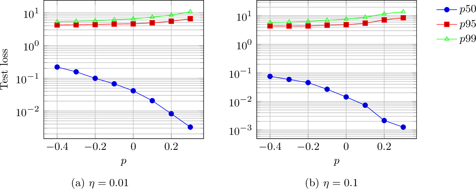
Under the larger learning rate \(\eta=0.1\), this phenomenon becomes more obvious. As \(p\) increases, the test median loss continues to decrease, but the tail loss worsens more strongly. When \(p=0.3\), the test \(p95\) loss reaches about \(8.51\), and the proportion of test samples with loss greater than \(5\) increases to about \(11.07\%\). This indicates that positive values of \(p\) more strongly reduce the loss of low-loss samples or core samples, while under a larger learning rate, this concentrated fitting further increases the risk of a heavier high-loss tail.
The clean train distribution shows a complementary trend. A larger \(p\) consistently produces lower training loss. For example, under \(\eta=0.01\), the clean train mean loss decreases from about \(0.092\) at \(p=-0.4\) to about \(0.0007\) at \(p=0.3\). Therefore, the worsening of the test tail is not caused by insufficient optimization. Instead, it shows that the fitting priority has been reallocated. A larger \(p\) strengthens the fitting of most training samples, but this concentrated fitting does not transfer uniformly to all test samples. In other words, the model fits easy samples first while reducing its fitting of hard samples.
These results directly refute the monotonic explanation that a smaller \(p\) must lead to better generalization. A too-small \(p\) can reduce tail amplification, but it also weakens training-set fitting. A too-large \(p\) can fit the training set more aggressively, but it produces a heavier test tail. Therefore, the best performance often appears in an intermediate allocation region, where core-sample fitting and tail-sample preservation reach a relative balance.
4.1.3 Hard-sample Migration↩︎
To determine whether the loss-tail change is only a rescaling of the same hard samples or a real change in sample priority, this paper further compares the top-loss sample sets under different values of \(p\). We define the samples with the highest final loss, accounting for the top \(10\%\), as hard samples, and compute the Jaccard overlap between different hard-sample sets.
Figure 6 shows that hard-sample sets are neither randomly changing nor fixed. On the test set, adjacent values of \(p\) have moderate overlap, with Jaccard values of about \(0.43\)–\(0.49\). The most distant settings, \(p=-0.4\) and \(p=0.3\), have an overlap of about \(0.35\). This indicates that part of the hard samples in the test tail comes from the data itself. Some samples are relatively hard under most optimization settings.

However, the overlap on the clean train set is clearly lower. Under \(\eta=0.01\), the Jaccard overlap between adjacent values of \(p\) is about \(0.16\)–\(0.29\), while the overlap between \(p=-0.4\) and \(p=0.3\) decreases to about \(0.125\). Similar results are also observed under \(\eta=0.1\). The low overlap on the training set shows that \(p\) changes which samples remain in the high-loss tail during training. Therefore, \(p\) does not only rescale the loss distribution. It also changes sample-level optimization priority.
This observation is key evidence for the information allocation perspective. If changing \(p\) only scaled the loss globally, the identity of hard samples should remain mostly stable. However, the experiments show that hard samples migrate with changes in \(p\), especially on the clean train set. This means that under different preconditioning exponents, the optimizer allocates fitting capacity to different sample sets.
4.1.4 Interaction with Learning-rate Decay↩︎
Although \(p\) is fixed in each run, all runs use the same cosine annealing schedule for the learning rate. The experiment can therefore also discuss, at a phenomenological level, how the learning rate affects training. We further observe that the weight-to-bias gradient structure changes with the learning-rate schedule. In most runs, as training proceeds, the gradient norms of both weight and bias decrease, but the bias gradient decreases faster. Therefore, the global \(G_w/G_b\) often increases in the later training stage.
This phenomenon provides additional evidence that weight–bias allocation is not an isolated effect of \(p\), but a real observable signal in optimization dynamics. It is affected by many training hyperparameters. When the learning rate is small, training tends to pay relatively more attention to the bias layer, which corresponds to model calibration. That is, a small learning rate does not only make parameters more stable in the conventional sense. It also reduces the training degree of weight parameters and tends to fix them, while relatively increasing the role of the bias layer in searching for decision boundaries. From the perspective of information allocation dynamics, this explains why learning-rate decay is necessary.
Therefore, \(p\) and learning-rate scheduling can be understood as two interacting sources of information allocation. The exponent \(p\) explicitly changes the channel gain under EMA preconditioning, while learning-rate decay changes the training stage and the remaining gradient demand. Their joint effect can be observed in the weight–bias gradient ratio and the sample-level loss distribution.
4.1.5 Summary↩︎
The results in this subsection support four conclusions.
First, the allocation exponent \(p\) systematically changes the global weight-to-bias gradient norm ratio, and this trend is stable under both learning-rate settings.
Second, by changing the global weight-to-bias update ratio, \(p\) reshapes the sample-level loss distribution. A larger \(p\) reduces the median loss but increases the high-loss tail, especially under a larger learning rate.
Third, the hard-sample overlap analysis shows that different values of \(p\) produce different hard-sample sets, especially on the clean train set. These results show that \(p\) controls not only the optimization magnitude, but also how optimization is distributed across parameter groups and samples.
Fourth, the learning-rate analysis shows that different values of \(p\) and different learning rates both affect the global weight-to-bias gradient norm ratio. This suggests that optimizer implicit bias under the information allocation perspective has multiple sources. Later studies should fully consider the differential forms and gradient propagation relations of different layers.
Taken together, these observations provide empirical evidence for the information allocation perspective proposed in this paper. The exponent \(p\) is not a simple scalar interpolation between SGD-like and Adam-like behavior. It serves as a control variable that changes how residual information is allocated across parameters and samples during training.
4.2 Validation of Dynamic Information Allocation in Facial Expression Recognition↩︎
To further verify the effectiveness of the information allocation mechanism in practical tasks, this paper tests dynamic \(p\) scheduling on facial expression recognition tasks based on PosterV2. Different from fixed-\(p\) optimization, dynamic \(p\) allows the optimizer to adjust the information allocation ratio in the parameter update process according to the training stage, and therefore adapt to the data-distribution characteristics of different tasks.
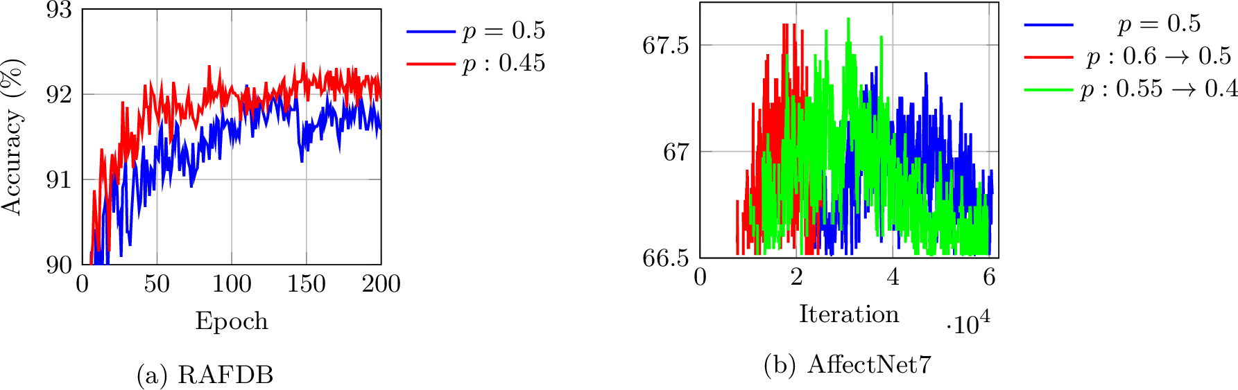
First, we conduct experiments on the RAFDB dataset. As shown in Fig. 7, the original training strategy (Origin, \(p=0.5\)) reaches a best accuracy of \(92.21\%\), while the dynamic information allocation strategy improves the accuracy to \(92.37\%\). In this experiment, \(p\) gradually decreases from \(0.45\) to \(0.35\). Since RAFDB has a relatively limited data scale, its weight-related information coverage is also limited. In this case, bias calibration becomes more important for the small dataset. The results show that properly decreasing \(p\) in the later training stage can further adjust the optimization focus and improve generalization.
On the more challenging AffectNet7 dataset, dynamic information allocation shows a clearer advantage. This dataset contains larger intra-class variation and more complex expression patterns, so the model needs to balance main representation learning and hard-sample optimization. As shown in Fig. 7, the fixed-\(p=0.5\) baseline reaches a best accuracy of \(67.49\%\). In comparison, the dynamic strategy that decreases \(p\) from \(0.6\) to \(0.5\) improves the best accuracy to \(67.61\%\). At the same time, the dynamic strategy that changes \(p\) between \(0.6\) and \(0.5\) also shows faster convergence.
In particular, compared with the fixed-\(p=0.5\) training process, the dynamic \(p\) strategy reaches a higher best accuracy with about half of the training steps. This shows that dynamic information allocation can improve not only final performance but also optimization efficiency. A possible reason is that AffectNet7 has a larger data scale and more effective weight-related information. In the early training stage, a larger \(p\) tends to focus optimization on stable and dominant features, and does not need to pay excessive attention to bias. This can accelerate the construction of the overall weight representation. As training proceeds, decreasing \(p\) can increase attention to hard samples and boundary information, and further refine the bias decision boundary.
These results show that the optimal information allocation strategy depends on the data characteristics of the specific task. For RAFDB, decreasing \(p\) is sufficient to bring gains. For AffectNet7, because the task complexity is higher, a clearer change in information allocation is needed. Therefore, dynamic \(p\) scheduling provides a way to adjust optimizer implicit bias according to task demands, so that the optimization process can adapt to the information needs of different data distributions.