Measuring Intelligence Beyond Human Scale
January 01, 1970
Abstract
How can we measure intelligence beyond human capability?
Human-authored benchmarks saturate, and above human capability, examiners may not know which tasks are both hard and verifiable. We argue that this difficulty is inherent to absolute-scale evaluation and propose a new paradigm based on relative measurement
in which models generate public challenges that separate other systems. Aggregating these outcomes yields an adversarial psychometric rating system that can scale with the systems being measured. We describe practical protocols that reduce incentives for
private-information attacks, support judge-free adjudication, and naturally scale with agent capabilities. We instantiate the framework across verifiable and open-ended, non-verifiable domains, illustrating how model-generated evaluation can continue to
measure systems beyond the human frontier.
1 Introduction↩︎
How should intelligence be measured? The question is older than the study of artificial intelligence.
The modern scientific study of intelligence began with the work of Charles Spearman [1]. Spearman observed that individuals who performed well on one cognitive test tended also to perform well on many others, a phenomenon now known as the positive manifold. He hypothesized that these positive correlations were explained by a single latent factor, which he called general intelligence (g). This marked a fundamental shift from viewing intelligence as a collection of observable abilities to modeling it as a latent statistical variable inferred from observable behavior, laying the foundations of modern psychometrics. Interestingly, this is also the seed of factor analysis in statistics.
Later item-response models made the measurement problem more explicit by jointly modeling subject ability and item difficulty. In the simplest Rasch model [2], the probability that a subject with ability \(\theta\) correctly answers an item of difficulty \(b\), and \(\sigma\) is the logistic function, is \[\Pr[\text{correct}]=\sigma( \theta - b).\]
This tradition has two important features. First, intelligence is measured through performance on tasks rather than defined independently of behavior. Second, the tasks are designed by human examiners, which is natural for human populations.
Most AI benchmarks inherit this psychometric structure. Systems are evaluated on tasks supplied by humans or environments fixed in advance: game environments, broad academic benchmarks and so on [3]–[10]. This becomes a scaling problem at the frontier: benchmarks saturate, and new ones require humans to generate tasks that are difficult and verifiable. Above human expert level, the bottleneck is not only the number of questions, but the examiner’s ability to formulate discriminating questions.
1.0.0.1 A different approach to measuring intelligence.
A different starting point is relative measurement. Turing’s imitation game measures machine intelligence by comparison with human behavior before a human judge, rather than by an absolute score on a fixed test [11]. Modern pairwise preference and arena methods similarly compare systems through judged interactions [12], [13]. These protocols point toward relative evaluation, but the tasks or judgments are still largely human-supplied. A notable exception is MathDuels [14], which explores model-generated mathematical pairwise challenges as an evaluation primitive.
However, purely pairwise comparative protocols are vulnerable to failure modes that can make the resulting signal uninformative. A model may exploit private information, construct trapdoor tasks, or target one particular weakness of a single opponent rather than reveal a general capability distinction, see more details in section 2.1.
We propose a model-generated and separative approach to intelligence evaluation, which we call adversarial psychometrics. While classical psychometrics measures intelligence by how well subjects solve examiner-designed tasks, adversarial psychometrics evaluates a model’s ability to discover capability boundaries among other systems. A model demonstrates superior intelligence by constructing challenges that separate a population of solvers.
Our central move is to replace pairwise comparison with separative measurement. A challenge is evaluated not by whether it defeats one opponent, but by the variance it induces across a population of solvers. This shift rewards proposers for identifying distinctions across systems, rather than for exploiting specific weaknesses of a target. By evaluating systems on their capacity to discover such capability gaps, we obtain a richer statistical signal that can scale beyond the human frontier and can support sparse, or even judge-free, adjudication.
Paper overview. The paper proceeds in three stages. First, we show that natural pairwise challenge protocols are fundamentally susceptible to private-information and trapdoor attacks, motivating a new one-to-many formulation. Second, we develop the separative psychometric framework, including its scoring rule, adaptive weighting, and judge-sparse adjudication mechanisms. Third, we demonstrate the framework empirically across verifiable and open-ended, non-verifiable domains, showing that model-generated evaluation can continue to discriminate between systems beyond the human frontier.
1.1 Relation to existing work↩︎
Psychometric and adaptive-testing models infer latent ability from responses to diagnostic items designed and administered by human examiners [1], [2], [15], [16]. Paired-comparison systems such as Bradley–Terry, Elo, and TrueSkill infer relative skill from sparse pairwise outcomes and provide principled methods for rating and uncertainty estimation [17]–[19]. Modern AI evaluation has focused on benchmark construction, contamination resistance, frontier-level difficulty, dynamic task collection, and pairwise comparison, including MMLU, BIG-Bench, HELM, ARC, LiveBench, FrontierMath, Humanity’s Last Exam, Dynabench, MT-Bench, and Chatbot Arena [3]–[10], [12], [13].
MathDuels [14] is particularly related to our work. It proposes a mathematical self-play benchmark in which models act as both problem posers and solvers. Our work shares the idea that task generation itself is a measurable capability, but differs in several respects: we study arbitrary domains rather than mathematics, develop a psychometric framework based on separations rather than dueling, design judge-free mechanisms, and focus on scalable measurement of capability beyond the human frontier.
Relation to Scalable Oversight. The scalable oversight problem asks: how do we obtain reliable supervision for systems whose competence exceeds that of their supervisors [20], [21]. Existing proposed mechanisms include debate, in which models argue opposing answers before a weaker judge [22]; weak-to-strong generalization, in which a weak supervisor elicits a stronger model’s latent ability [23]; and sandwiching or recursive-critique protocols that test whether verifying an answer is easier than producing one [24]. Our work shares the same motivation: human evaluators may eventually be unable to author or verify sufficiently discriminating tasks. However, whereas scalable oversight seeks reliable supervision of individual systems, we focus on comparative measurement.
Relation to interactive proofs and complexity theory. There is also a conceptual connection to multi-prover interactive proofs (MIPs). In an MIP, a bounded verifier extracts reliable evidence by comparing the behavior of multiple provers; the theorem of [25] that \(\mathsf{MIP} = \mathsf{NEXP}\) demonstrated the remarkable power of such multi-agent verification. Our protocol is not an MIP in the formal sense: we do not provide completeness or soundness guarantees for a fixed language, nor do we assume a polynomial-time verifier. However, we have the shared idea that multiple agents can reveal information that a single agent cannot. Whereas MIPs use cross-prover consistency to verify mathematical claims, adversarial psychometrics uses cross-model disagreement to measure capability boundaries.
2 Warm-up: pairwise intelligence tournaments↩︎
A natural first attempt is a pairwise intelligence tournament. Given two systems \(i\) and \(j\), system \(i\) is asked to produce a challenge that it can solve but system \(j\) cannot. The challenge must be publicly specified and objectively resolvable. System \(j\) then submits an answer under the same resource budget, and the outcome is recorded as a win for \(i\) if \(i\)’s answer is correct and \(j\)’s answer is incorrect.
Over many such matches, the outcomes define a directed comparison graph: an edge \(i \to j\) indicates that system \(i\) found a challenge separating itself from system \(j\). In principle, this graph could be aggregated by any standard paired-comparison model, such as Bradley–Terry, Elo, or TrueSkill. For example, a Bradley–Terry model assigns each system a latent score \(\theta_i\) and models \[\Pr(i \text{ beats } j) = \sigma(\theta_i-\theta_j).\] Equivalently, one could maintain Elo-style online ratings from the same pairwise outcomes.
This gives a simple self-scaling measurement scheme: stronger systems should be able to find challenges that separate themselves from weaker systems, and the rating scale evolves with the population being measured. However, the pairwise formulation has fundamental flaws.
2.1 Caveats of pairwise protocols↩︎
The first difficulty is that this naive protocol rewards separation from a single opponent, and therefore creates incentives to exploit asymmetric information rather than capability. The simplest attack is a private-state question, such as “which bit am I thinking of?”
One might try to rule out such private or otherwise unfair questions. But the same problem can arise even in questions that appear fair. For example, a challenger can generate two large primes, publish their product, and ask for its factorization. Under the same resource budget the task may be hopeless for the solver, while the challenger has “solved” it only because it inserted the trapdoor during construction.
The common issue is that the challenger possesses information unavailable to the solver: in one case a private state, and in the other an algorithmic backdoor. Such separations need not reflect superior intelligence.
A second problem is adjudication. Even if private-information and trapdoor questions are formally disallowed, the protocol still requires someone to decide whether a challenge is admissible and whether its proposed resolution is correct. Without an external judge, the parties’ own reports can enforce agreement but not truth. Penalties for disagreement may induce the players to agree, but they cannot distinguish the truthful resolution from a biased one. Thus pairwise protocols either rely on external adjudication, which limits scalability, or remain manipulable.
The key observation is that private information and trapdoors are powerful mainly because the challenger is trying to fool a single opponent. If the same challenge is posed simultaneously to many independently trained systems, the challenge must separate a population rather than exploit hidden information about one solver. This motivates the one-to-many protocol developed next.
3 The Basic Challenge Protocol↩︎
We call our novel ranking protocol SepaRank , and its basic description is as follows. A proposer submits a binary question with answers A and B2. Each solver returns an answer and a confidence, equivalently a posterior probability \(p_i\) assigned to answer A. The proposer is rewarded for inducing high variance in the values \(\{p_i\}\) across solvers.
No restriction is placed on the semantic content of the question. The question may be factual, mathematical, philosophical, subjective, future-contingent, or otherwise difficult to resolve externally. Different resolution rules therefore induce different interpretations of the score, a distinction explored empirically in Section 4.
This changes the incentive relative to pairwise challenge protocols. The question “which bit am I thinking of?” no longer succeeds: a calibrated solver has no evidence and should report \(p_i=\frac{1}{2}\), so the variance is small. Likewise, a trapdoor-ed factoring instance does not help merely because the proposer generated the primes; the proposer anyways is not required to solve the problem, and if the problem is too hard, calibrated reports again concentrate near \(\frac{1}{2}\). The proposer succeeds only by finding questions that genuinely separate the audience.
We use variance as the proposer objective for simplicity. Other separation objectives are also possible, such as the empirical entropy of the distribution of reports or a weighted Jensen–Shannon divergence, which measures how much information a report carries about which solver produced it.
3.1 Protocol↩︎
We evaluate systems in two roles: proposer and solver. In each round, a proposer submits a binary question with answers \(A\) or \(B\) and a committed answer \(\hat{y}\in\{0,1\}\), where \(\hat{y}=1\) asserts that \(A\) is correct and \(\hat{y}=0\) asserts that \(B\) is correct.
All solvers receive the same question, resource budget, and resolution rule. In the basic proposer-answer version, the resolved answer is the proposer’s commitment, \(y=\hat{y}\). Other variants may resolve \(y\) by deterministic execution, an external verifier, random audit, or audience consensus. Thus, when \(y\) is externally verifiable, solver loss measures accuracy with respect to a public truth; when \(y\) is proposer-committed or consensus-based, it measures calibration relative to that resolution rule.
Each solver \(i\) returns an answer, \(A\) or \(B\), and a confidence \(c_i\in[1/2,1]\). We convert this into the solver’s reported probability of \(A\): \[p_i = \begin{cases} c_i, & \text{if the solver answers } A,\\ 1-c_i, & \text{if the solver answers } B. \end{cases}\] Thus ignorance corresponds to \(p_i=1/2\), confident belief in \(A\) to \(p_i\approx 1\), and confident belief in \(B\) to \(p_i\approx 0\). The answer-and-confidence pair is one convenient interface, but the two parameterizations are interchangeable, and in our implementation each solver simply reports the probability \(p_i\in[0,1]\) as a single numeric field in its reply, elicited zero-shot by prompting; no model is fine-tuned, and the scoring below applies to the reported number as is. The proposer is rewarded for separating the audience: \[\mathrm{Score} = 4\,\operatorname{Var}(p) = \frac{4}{m}\sum_{i=1}^m (p_i-\bar p)^2, \;\;\;\bar p=\frac{1}{m}\sum_{i=1}^m p_i.\] The factor \(4\) normalizes the score to lie in \([0,1]\). A private-state question such as “which bit am I thinking of?” receives essentially zero score, since calibrated solvers should all report \(p_i=1/2\). Similarly, a trapdoored instance does not help unless the public challenge itself gives some solvers a basis for confidence.
Solvers are scored separately against the resolved answer by a proper scoring rule. For example, with Brier loss, \[\mathrm{Loss}_i=(p_i-y)^2,\] where \(y=1\) if the resolved answer is \(A\), and \(y=0\) if the resolved answer is \(B\). This gives solvers an incentive to report calibrated beliefs about the resolved answer, while proposers are rewarded for finding questions on which calibrated beliefs differ.
Scores accumulate round by round. In a round, a system obtains a proposer quantity \(P\), the \(\operatorname{Score}=4\operatorname{Var}(p)\) of the challenge it authored, and a solver quantity \(Q\), the negative of its mean Brier loss over the challenges it was drawn to solve that round. Each quantity is standardized across the population within the round, and the round score averages the two roles, \[g_i^{(r)} \;=\; \tfrac12\,z\!\big(P_i^{(r)}\big) \;+\;\tfrac12\,z\!\big(Q_i^{(r)}\big), \qquad z(x_i)=\frac{x_i-\bar x}{\max\!\big(\operatorname{sd}(x),\,z_{\min}\big)}\] so the two roles contribute equally and every round carries equal weight regardless of its raw spread. Here \(\operatorname{sd}\) is the population standard deviation across the systems that hold the quantity that round, \(z_{\min}\) is a small floor (we use \(z_{\min}=0.02\)) so that a round with negligible spread moves no one, and \(z(x_i)=0\) whenever fewer than two systems hold the quantity or the spread is zero. A system not drawn to solve in a round has no \(Q\) and contributes \(z(Q^{(r)})=0\); a proposer whose sub-round yields no usable panel contributes \(z(P^{(r)})=0\).
The rating after \(R\) rounds is the running total \[G_i \;=\; \sum_{r=1}^{R} g_i^{(r)},\] and each system seeks to maximize \(G_i\). We standardize within rounds and sum, rather than standardizing batch means once at the end, because per-round increments keep rounds exchangeable and directly drive the adaptive weighting of Section 3.3; the leaderboards of Section 4 rank by exactly this \(G\).
3.2 Thresholding and probability amplification↩︎
A subtle failure mode of the variance objective is probability amplification. A proposer can replace a single binary question by the conjunction of \(k\) binary questions. This may be a legitimate way to create a harder challenge: solving all \(k\) components can require greater reasoning, knowledge, or computation, especially under fixed resource constraints. However, it can also mechanically push reported probabilities toward the extremes of zero and one. Thus raw variance in the reported probabilities \(p_i\) may reflect the logical thresholding effect of the question, not only a sharper capability separation.
A simple alternative is to compute separation after coarsening the reported probabilities. For each solver \(i\), define \[\widehat p_i = \Pi_{\{0,1/2,1\}}(p_i),\] where \(\Pi_{\{0,1/2,1\}}\) rounds to the nearest point in \(\{0,1/2,1\}\). Thus reports near \(0\) are treated as confident belief in \(B\), reports near \(1/2\) as ignorance, and reports near \(1\) as confident belief in \(A\).
The proposer score is then computed from the rounded reports: \[\mathrm{Score}_{\rm prop} = 4\,\operatorname{Var}(\widehat p).\] This preserves the binary-question format while reducing sensitivity to probability amplification. A conjunction scores highly only if it creates categorical separation among solvers: some are confident in one answer, some are confident in the other, or some remain genuinely uncertain.
We do not apply this coarsening in the experiments of Section 4, which score the raw variance; it is included as an available mitigation when probability amplification is a concern.
3.3 Clustering failure↩︎
The unweighted variance objective can suffer from a frontier-clustering failure. After several rounds, the protocol may identify a set of systems that clearly separate themselves from the rest. At that point, proposers can continue to earn high score by separating the frontier from the bulk, even though this no longer resolves distinctions within the frontier.
To make the measurement adaptive, we replace the uniform variance by a weighted variance whose weights evolve across phases. Let \(w_i^{(r)}\ge 0\) denote the weight assigned to solver \(i\) in phase \(r\), normalized so that \[\sum_{i=1}^m w_i^{(r)}=1.\] Initially, \[w_i^{(0)}=\frac{1}{m}.\] For a challenge in phase \(r\), define \[\bar p_w=\sum_{i=1}^m w_i^{(r)}p_i, \qquad \operatorname{Var}_w(p) = \sum_{i=1}^m w_i^{(r)}(p_i-\bar p_w)^2 .\] The proposer score becomes \[\mathrm{Score}=4\,\operatorname{Var}_w(p).\] The weighting can equivalently enter through sampling rather than analytically: draw each challenge’s panel of \(k\) solvers without replacement with probability proportional to \(w^{(r)}\), and score the ordinary unweighted variance over the sampled panel. In expectation this matches the weighted objective while keeping every panel small and the score formula unchanged, and it is the form used in the experiments of Section 4. If the coarsening defense against boosting is used, \(p_i\) is replaced by \(\widehat p_i\) in the same formula.
After each phase, ratings are refit and the weights are updated toward the systems with the highest current overall scores. A simple multiplicative-weights update is \[\widetilde{w}_i^{(r+1)} = w_i^{(r)}\exp\big(\eta\, G_i^{(r)}\big), \qquad w_i^{(r+1)} = (1-\epsilon) \frac{\widetilde{w}_i^{(r+1)}}{\sum_{j=1}^m \widetilde{w}_j^{(r+1)}} + \frac{\epsilon}{m},\] where \(G_i^{(r)}\) is the sum of system \(i\)’s round scores \(g_i\) (Section 3) over phase \(r\) alone, not cumulative across phases. Here \(\eta>0\) is a small adaptation rate and \(\epsilon>0\) prevents any system from receiving zero weight. In order to reduce noise, we can update the weights every several rounds, rather than every single round, or alternatively use a moving average instead of instantenous scores.
Thus early rounds measure broad separations across the full population, while later rounds increasingly reward challenges that distinguish among the current frontier. A question that only separates already-strong systems from already-weak systems receives decreasing reward; to score highly, a proposer must eventually find challenges on which the high-performing systems themselves differ.
The latter point suggests that adaptive weighting can encourage a form of question diversity. However, the open nature of the protocol does not by itself guarantee novelty. Since all agents observe prior questions and outcomes, successful templates can be copied. Thus public history reduces the value of exact answer-key memorization but may also create free-riding on discovered templates. This motivates adding an explicit novelty term or duplication penalty in future versions of the mechanism.
3.4 Resolution rules and optional adjudication↩︎
The SepaRank protocol separates the scoring mechanism from the resolution rule. In every round, solvers submit probabilities \(p_i\), the proposer is scored by the induced separation among those probabilities, and solvers are scored by a proper scoring rule against a resolved bit \(y\). The resolution rule specifies how \(y\) is obtained.
In mechanically verifiable domains, \(y\) may be determined by executing a program, checking a proof, or verifying a certificate. In this case solver loss measures accuracy with respect to an objective public truth. In non-verifiable domains, \(y\) may instead be the proposer’s committed answer. This version is fully judge-free, but the solver task becomes predicting the proposer’s committed resolution. The incentives this creates for the proposer, and the extent to which models exploit them, are measured in Section 4.4.
Although false commitments may increase disagreement in the short run, they should eventually erode trust. As a proposer becomes less reliable, calibrated solvers ought to hedge toward \(\frac{1}{2}\), reducing the proposer’s variance reward and creating a long-run incentive for honest commitments.
A third judge-free option is consensus resolution, in which \(y\) is determined by the aggregate response of the solver population. This measures agreement with the population and can reveal collective blind spots, but may also introduce herding or majority-error effects.
Thus the proposer score always has the same meaning: it measures the ability to find questions on which the solver population separates. The solver score, however, is interpreted relative to the chosen resolution rule.
Although the basic protocol can be run without a judge, external adjudication can be added as an optional layer when available. For example, a proposer may submit a challenge together with a committed answer or certificate. Solvers first submit their answers and confidences without seeing one another’s reports. After the reports are locked, the proposed resolution is revealed. The round may then be accepted automatically, randomly audited, or escalated to a judge if a solver objects by posting a bond. If adjudication contradicts a party’s commitment, that party pays an additional penalty: the proposer if the challenge is inadmissible or the committed resolution is wrong, and the objecting solver if the objection is wrong.
This judge-sparse variant is not required for the core measurement protocol, but it provides a useful bridge between fully verifiable and fully judge-free settings. When external verification is cheap, it can anchor the benchmark to objective truth. When verification is expensive or unavailable, the same scoring mechanism can continue to operate using committed or consensus resolution.
Appendix 10 gives examples of task domains and suitable resolution mechanisms.
4 Experiments↩︎
We experimentally implement the protocol as described above, with the following variations. The proposer writes an artifact, which is either an executable Python program, namely a no-argument main() returning \(0\) or \(1\), or a plain yes/no question in natural language. The resolution rule then fixes the bit \(y\) that solvers are graded against.
A program can be resolved by the bit it returns when executed in a sandbox (execute) or by the bit the proposer commits alongside it (committed). A general question which is not generally verifiable, is resolved by the committed bit of the proposer or by the majority vote of the panel (consensus).
We label these four variations PE (program-executed), PC (program-committed), QC (question-committed) and QN (question-consensus), based on the artifact type and resolution procedure.
In this section, we present our experimental results on the two commit variations (PC and QC).
| Model | Provider | Reasoning configuration |
|---|---|---|
| gpt-5.5, gpt-5.4 | OpenAI | reasoning model, reasoning_effort=low |
| gpt-5.4-mini, gpt-5.4-nano | OpenAI | reasoning model, reasoning_effort=low |
| gpt-4o-mini | OpenAI | non-reasoning chat model |
| opus-4.8, sonnet-4.6 | Anthropic | adaptive extended thinking, effort=low |
| haiku-4.5 | Anthropic | extended thinking off |
| qwen3.7-max | Alibaba | thinking disabled |
| kimi-k2.7 | Moonshot AI | thinking disabled |
| deepseek-v4-pro | DeepSeek | thinking disabled |
For these two variations, we run ten independent games, every game fields the same \(N{=}11\) contemporary models under stable pseudonyms, drawn from five providers to span a wide and known capability range. Table 1 gives the exact reasoning configuration of each model. A game lasts \(R{=}20\) rounds and in each round every model authors one challenge and a panel of \(k{=}5\) solvers is drawn from the ten other models per challenge. Prompts disclose the entire mechanism including the scoring formulas, the resolution rule, the adaptive weighting, and a transcript of 5 recent rounds. A proposal that violates an enforced rule is voided and scores \(-1\).
In the program variation admissibility is machine checked (standard library only, resource limits, determinism across two executions). In the question arm the content rules of Section 3 are stated to the models but no judge inspects question content. Appendix 8 lists the complete parameter set, the failure and quorum rules, and the information structure of the prompts.
Scoring follows Section 3: a proposer earns \(P=4\operatorname{Var}(p)\) for the disagreement it induces across its panel, and a solver pays the Brier loss \(\ell=(p-y)^2\) against the resolved bit. To aggregate the two roles on a common scale, each round both quantities are standardized across the field and averaged, \[g \;=\; \tfrac12\, z(P) \;+\; \tfrac12\, z(Q),\] where \(Q\) is the negative of the model’s mean solver loss that round, \(z\) is the z-score across the eleven players, and the z-score divisor is floored at \(0.02\). A model’s rating is the total score \(G=\sum_r g_r\) of Section 3; it is the ranking statistic everywhere below. The adaptive weights of Section 3.3 are driven by the same increments, updated every five rounds, and serve only to bias panel sampling toward stronger solvers; they play no role in the rating itself.
Tables report the mean of \(G\) across the ten games of an arm with two-sided \(95\%\) \(t\)-intervals. Statements that one model outranks an adjacent one are paired \(t\)-tests on per-game score differences.
4.1 Rankings under committed resolution↩︎
Tables 2 and 3 give the two leaderboards. In the program arm the two frontier OpenAI models separate from the field and from each other: gpt-5.5 finishes first in nine of ten games, its paired advantage over gpt-5.4 is significant (\(\Delta G = 3.1\), \(p=0.008\)), and gpt-5.4’s advantage over the third-place model is larger still (\(\Delta G = 6.4\) over qwen3.7-max, \(p=0.006\)).
For the question arm, its top pair is statistically indistinguishable (\(p=0.76\)). Only two separations reach significance, gpt-5.4-nano over kimi-k2.7 (\(p=0.020\)) and deepseek-v4-pro over gpt-4o-mini (\(p=0.001\)).
The extremes are stable in both arms: the frontier pair leads both boards and gpt-4o-mini anchors the bottom of both.
Looking at the solver losses, we find that models almost never hedge. The mean distance of a report from one half, \(|p-\tfrac12|\), lies between \(0.39\) and \(0.50\) for every model in both arms, so reports are close to binary and the Brier loss is governed almost entirely by directional accuracy.
We conclude that the weakest solvers are not merely ignorant but also miscalibrated. For example, in the question arm gpt-4o-mini answers on the wrong side on \(40\%\) of its reports while keeping a mean extremity of \(0.46\), leaving its Brier loss (\(0.388\)) well above the \(0.25\) of a solver that answers one half to every challenge.
The strongest models are both directionally correct and are the most calibrated. gpt-5.4’s mean extremity, \(0.40\) to \(0.41\), is the lowest among engaged players in both arms. The proper scoring rule is doing its intended work, separating knowing from knowing that one does not know, and the failure of weak models to declare when they are unsure is itself a capability signal.
| # | Model | \(G\) | \(P\) | \(\ell\) | \(w\) | Honesty (%) |
|---|---|---|---|---|---|---|
| 1 | gpt-5.5 | \(+12.9\pm1.5\) | \(0.384\pm0.025\) | \(0.054\pm0.010\) | \(0.416\) | \(59.0\pm9.4\) |
| 2 | gpt-5.4 | \(+9.7\pm1.8\) | \(0.367\pm0.028\) | \(0.082\pm0.010\) | \(0.240\) | \(79.5\pm4.8\) |
| 3 | qwen3.7-max | \(+3.3\pm2.8\) | \(0.194\pm0.022\) | \(0.107\pm0.017\) | \(0.090\) | \(99.0\pm0.7\) |
| 4 | gpt-5.4-mini | \(+1.3\pm2.3\) | \(0.187\pm0.021\) | \(0.126\pm0.014\) | \(0.055\) | \(94.5\pm1.9\) |
| 5 | opus-4.8 | \(-0.4\pm2.1\) | \(0.086\pm0.020\) | \(0.095\pm0.010\) | \(0.043\) | \(97.5\pm0.8\) |
| 6 | sonnet-4.6 | \(-1.0\pm2.0\) | \(0.093\pm0.024\) | \(0.122\pm0.012\) | \(0.041\) | \(94.4\pm2.2\) |
| 7 | haiku-4.5 | \(-4.3\pm2.1\) | \(0.078\pm0.020\) | \(0.169\pm0.022\) | \(0.024\) | \(90.1\pm3.2\) |
| 8 | gpt-5.4-nano | \(-4.6\pm2.2\) | \(0.122\pm0.014\) | \(0.178\pm0.013\) | \(0.024\) | \(94.5\pm1.9\) |
| 9 | kimi-k2.7 | \(-4.7\pm1.8\) | \(0.143\pm0.010\) | \(0.210\pm0.013\) | \(0.022\) | \(82.2\pm2.7\) |
| 10 | deepseek-v4-pro | \(-5.2\pm3.3\) | \(0.076\pm0.036\) | \(0.213\pm0.025\) | \(0.026\) | \(77.1\pm5.1\) |
| 11 | gpt-4o-mini | \(-6.9\pm2.2\) | \(0.068\pm0.020\) | \(0.254\pm0.017\) | \(0.019\) | \(89.5\pm3.3\) |
| # | Model | \(G\) | \(P\) | \(\ell\) | \(w\) |
|---|---|---|---|---|---|
| 1 | gpt-5.5 | \(+7.0\pm3.3\) | \(0.368\pm0.052\) | \(0.148\pm0.011\) | \(0.207\) |
| 2 | gpt-5.4 | \(+6.5\pm3.0\) | \(0.363\pm0.050\) | \(0.144\pm0.008\) | \(0.198\) |
| 3 | opus-4.8 | \(+4.4\pm3.2\) | \(0.324\pm0.034\) | \(0.187\pm0.031\) | \(0.140\) |
| 4 | qwen3.7-max | \(+2.8\pm2.5\) | \(0.319\pm0.051\) | \(0.197\pm0.017\) | \(0.090\) |
| 5 | sonnet-4.6 | \(+2.1\pm2.6\) | \(0.276\pm0.046\) | \(0.198\pm0.032\) | \(0.088\) |
| 6 | haiku-4.5 | \(+1.1\pm4.0\) | \(0.246\pm0.041\) | \(0.197\pm0.026\) | \(0.097\) |
| 7 | gpt-5.4-mini | \(+0.4\pm1.8\) | \(0.246\pm0.055\) | \(0.219\pm0.038\) | \(0.062\) |
| 8 | gpt-5.4-nano | \(-0.5\pm1.7\) | \(0.175\pm0.024\) | \(0.174\pm0.011\) | \(0.054\) |
| 9 | kimi-k2.7 | \(-4.8\pm3.3\) | \(0.171\pm0.026\) | \(0.253\pm0.024\) | \(0.030\) |
| 10 | deepseek-v4-pro | \(-5.6\pm2.1\) | \(0.278\pm0.045\) | \(0.335\pm0.030\) | \(0.023\) |
| 11 | gpt-4o-mini | \(-13.3\pm2.3\) | \(0.104\pm0.022\) | \(0.388\pm0.029\) | \(0.011\) |
4.2 Agreement between the arms↩︎
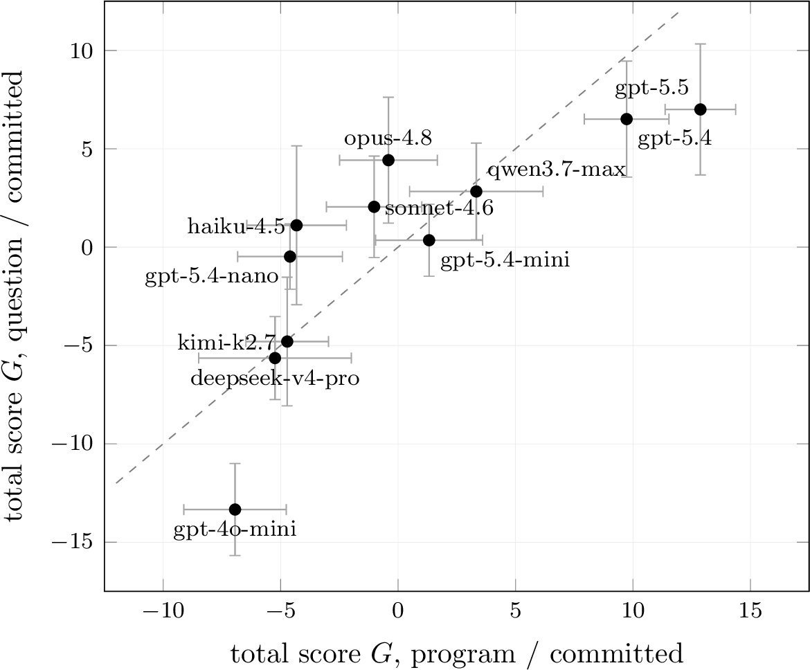
Figure 1 plots each model’s program-arm score against its question-arm score. The two arms agree on the overall ordering (Spearman \(\rho=0.93\), Pearson \(r=0.79\) across the eleven models) while disagreeing on individual models in an interpretable way. Models such as opus-4.8 are relatively stronger on questions, whereas the frontier OpenAI models sit below the diagonal, with relative advantage in challenges that involve verifiable deterministic computations.
4.3 Dynamics↩︎
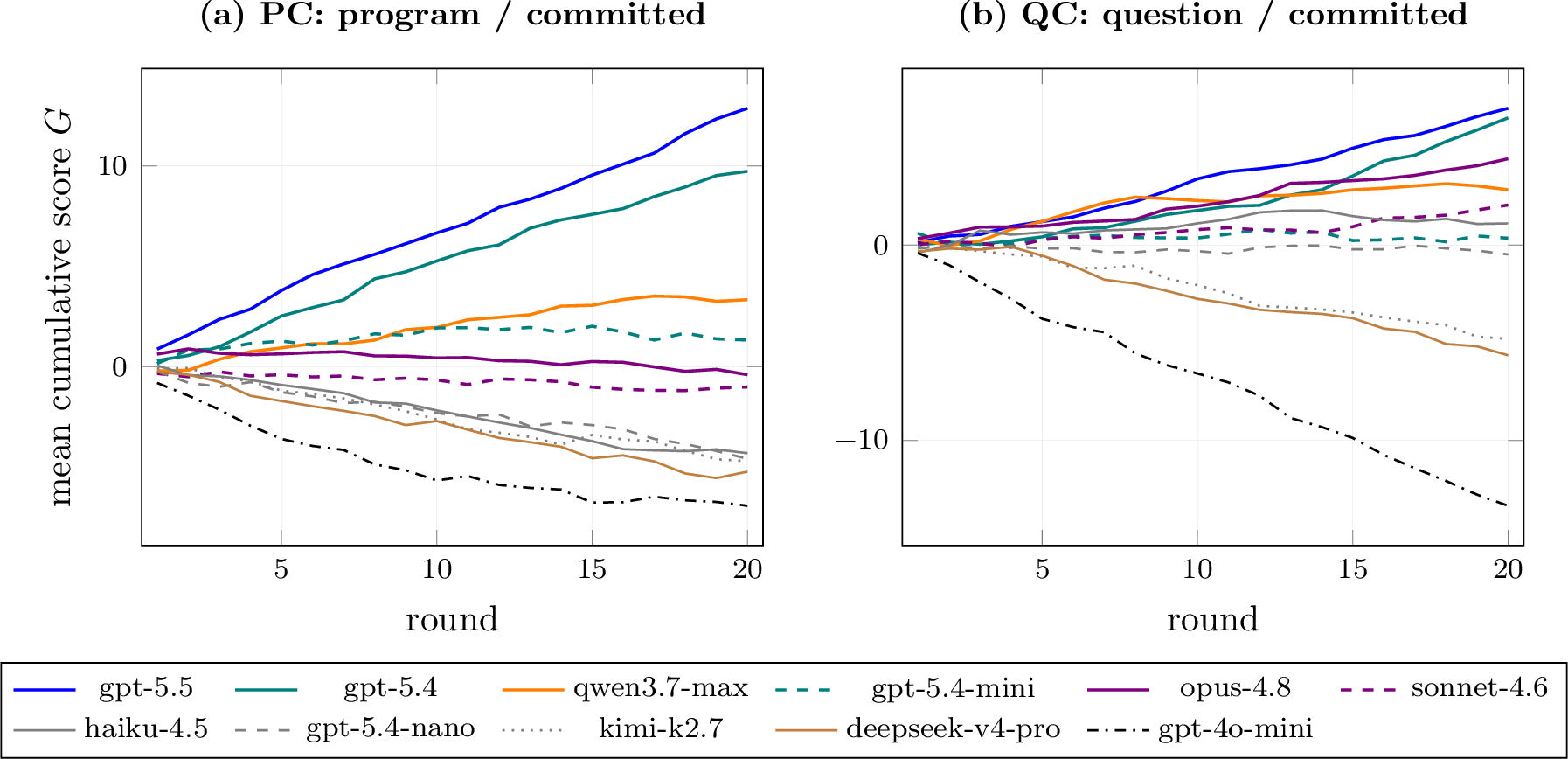
Figure 2 shows the mean dynamics over a single game. We observe that the scores of the leaders grow approximately linearly in general, indicating that the smart models have a steady per-round edge rather than a compounding one as the number of rounds played increases.
We also notice some models like opus-4.8 briefly peaking with second place in the PC arm but then decaying afterwards. One can interpret this opus-4.8 being a relatively stronger with a weaker pool of models, but once the adaptive weights kick in, it is less capable against a field of stronger models.
Opus-4.8’s weakness in the program-arm is counterintuitive to our priors on its capability. We find that its solving is excellent, and standardized across the field, its solver half contributes \(+2.2\) per game, third behind the two frontier OpenAI models, and its Brier loss (\(0.095\)) is likewise third best.
However, it falls short in authoring (\(-2.6\) per game, third worst). Looking at the transcripts, we determine that its challenges fail to divide the panel. On \(84.5\%\) of its valid programs every panelist answers on the correct side (the same figure is \(23.1\%\) for gpt-5.5 and \(33.7\%\) for gpt-5.4), so the variance reward pays it almost nothing (mean \(P=0.086\)). Opus-4.8’s writing style is visibly cooperative rather than adversarial. Ninety-two percent of its programs carry comments and \(70\%\) carry comments that narrate the computation or its result, against a \(3.5\%\) comment rate for gpt-5.4. Combined with a \(97.5\%\) honest commitment rate, its proposals amount to annotated exercises with reliable answers, which a field of this strength solves unanimously. Its five miscommitted proposals earned a mean reward of \(0.32\), nearly four times its average, an incentive it declines to engage in. In short, the committed program arm specifically penalizes transparent, honest authoring, and opus-4.8 is the model most committed to that style.
We also observe that the authoring pool itself is not stationary, because the models imitate one another through the public transcript. In the question arm the share of proposals that duplicate a question already asked earlier in the same game rises from \(3\%\) over the first five rounds to \(20\%\) over the last five. Duplicated questions earn a mean proposer reward of \(0.36\) against \(0.25\) for novel ones, because a question that split one panel usually splits the next. Free-riding on a discovered template can pay better better than discovery.
4.4 Honesty under committed resolution↩︎
Committed resolution makes misrepresentation a legal move since the resolved bit is whatever the proposer commits (and not necessarily matching what the program output actually is).
First, the population is largely honest. Across the ten games, \(87.0\%\) of the proposals commit the bit the program actually returns, and the rate is flat across rounds within a game.
Second, miscommitment pays. Dishonest proposals earn a mean proposer reward of \(0.36\) against \(0.15\) for honest ones. This arises plausibly because commitment that contradicts the program’s behavior manufactures disagreement between solvers that execute the code correctly and solvers that anticipate the deception.
Third, the strategy concentrates at the top. The arm’s winner, gpt-5.5, is also its least honest proposer at \(59.0\%\), and its deception is patterned rather than erratic. It reuses the same challenge template with an honest commitment in one round and a false commitment in another, so that a solver who recognizes the template from the public transcript still cannot infer the bit, and its honesty rate swings between \(45\%\) and \(73\%\) across batches of games while it wins throughout. By contrast qwen3.7-max commits honestly in \(198\) of \(200\) proposals and opus-4.8 in \(195\) of \(200\), and both are outranked.
The miscommitments of the weakest models arise differently. Deepseek-v4-pro (\(77\%\)) and kimi-k2.7 (\(82\%\)) also have the highest solver losses, consistent with failing to predict their own program rather than with strategy.
4.5 Defeating Exploits with Reasoning↩︎
Without mechanical checks on question quality, the non-verifiable setting is seemingly vulnerable to exploits: non-informative or trivial questions that still succeed in rewarding the questioner. If such questions become a long-term equilibrium, the protocol will collapse and no longer measure intelligence. Due to the open histories available to each model, successful attacks can be quickly copied, even by models that are not strong enough to discover them. This makes it essential that our protocol be designed so that these behaviors will not be optimal against rational opponents. Even so, there is no guarantee our current competitors are actually rational.
Providing agents with a chain-of-thought scratchpad allows us to verify that models understand these mechanics and rationally defeat exploits. This experiment compared the same suite of 11 models when instructed to reason until they were confident about their responses. For this set of tests, solvers could see the proposer for the currently posed question, allowing them to condition on previous proposer behavior.
| Model | Internal reasoning | Records | Total chars | Mean chars | Median chars |
|---|---|---|---|---|---|
| Kimi K2.7 | \(\times\) | 1,172 | 3,279,024 | 2798 | 790 |
| DeepSeek V4 Pro | \(\times\) | 1,065 | 3,083,278 | 2895 | 818 |
| Claude Haiku 4.5 | \(\times\) | 1,096 | 2,247,780 | 2051 | 1876 |
| GPT-5.4 | ✔ | 1,403 | 741,652 | 529 | 511 |
| Qwen3.7 Max | \(\times\) | 1,337 | 712,895 | 533 | 463 |
| GPT-5.5 | ✔ | 1,534 | 517,552 | 337 | 318 |
| Claude Sonnet 4.6 | ✔ | 1,255 | 474,958 | 378 | 124 |
| GPT-4o mini | \(\times\) | 846 | 400,417 | 473 | 429 |
| GPT-5.4 mini | ✔ | 1,140 | 232,450 | 204 | 181 |
| GPT-5.4 nano | ✔ | 957 | 225,525 | 236 | 221 |
| Claude Opus 4.8 | ✔ | 1,381 | 221,333 | 160 | 121 |
| Total | — | 13,186 | 12,136,864 | — | — |
One caveat to note is that some models had internal reasoning that could not be made visible and could not be turned off. These models did not need to do all of their thinking in the scratchpad, and the table shows that they made far less use of it. Table 4 shows that models without an internal chain-of-thought (Kimi, DeepSeek, Haiku) wrote far longer scratchpads than those whose internal reasoning could not be disabled and thus offloaded most of their thinking outside the scratchpad.
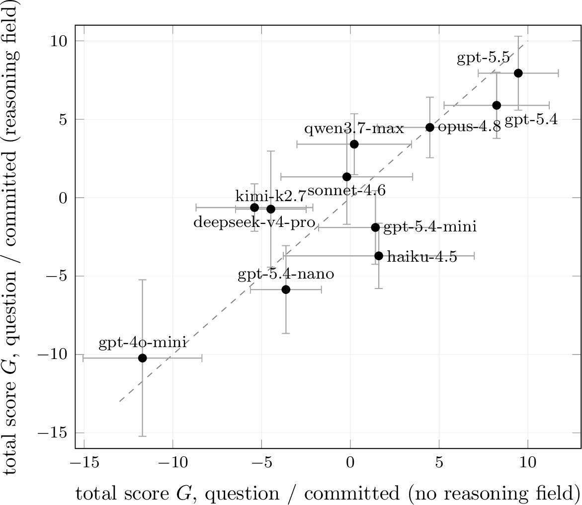
Figure 3 compares total scores with and without the reasoning field. Adding reasoning produces a ranking broadly similar to the no-reasoning arm (Spearman \(\rho=0.70\)). Kimi, DeepSeek, and Qwen show the clearest relative gains under reasoning (DeepSeek significantly, \(p=0.01\); Kimi and Qwen marginally), while Haiku and GPT-5.4-mini decline. Reasoning traces show Kimi and Qwen playing highly strategically (App.[trace:date],[trace:minimax]), which was likely not possible with zero thinking. Haiku’s counterintuitive decline coincides with a fall in its proposer score and its rate of false commitment: without reasoning, it selected difficult problems for which it often committed incorrect answers, whereas reasoning calibrated its proposals to its own capability.
Identity-based separation. The most obvious way for a questioner to induce high-variance responses is to simply demand it. Many powerful solvers reasoned that questions that ask players about their own pseudonym were not forbidden and would always vary between players. The basic question template here asks models whether their pseudonym is in one set of half the players or the other: e.g., does your pseudonym contain the letter ‘a’?.
This question exposes a lack of theory-of-self. Many models do not separate between a fact that is true for them and a fact that is true in general. Even though they are aware that the proposer committed a single correct answer, they believe this is the same as the correct answer relative to them. This occurs even among strong models, such as Opus 4.8 (App. [trace:naive]). Rational models realize that an identity-based question cannot have a true answer for the panel as a whole and choose to predict the proposer’s committed answer instead (App. [trace:identity]). This provides a massive solver payoff relative to naive answering.
Dishonest answer reporting. Within a single round, the proposer reward function does not depend on the answer committed by the proposer, only on the responses from the solvers. The committed bit only impacts solver rewards. Assuming naive solvers, if the committed answer is actually wrong, this will lower solver scores, especially for strong models that answer the question correctly. Therefore, there is an active disincentive to commit to the true answer.
This leads to exploits where models provide trivially easy questions and commit incorrectly, increasing the loss of their competitors. However, the open protocol means such behavior is self-defeating in the long run. Models consistently track the prior answer commitments made by a given questioner. For questioners with a history of erratic answer commits, capable models reason that the question is unpredictable: basically just, “What bit am I thinking of?” Therefore, they hedge and report probabilities close to 0.5, which is the exact mechanism designed to prevent such questions (App. [trace:minimax]). If the entire field is sufficiently rational, they will all do the same, reducing the proposer reward to 0. Therefore, models must be consistent in their honesty to maximize rewards in the long run. Comparing this to the dishonesty observed when questioners were hidden shows that models act rationally under the open protocol.
Intractable problems. There is no upper bound on question difficulty, since a proposer is never punished for an incorrect answer and need not know it. When a question is genuinely beyond every model, such as a very deep digit of \(\pi\), weaker models correctly reason that they cannot predict it and hedge toward \(0.5\) (App. [trace:intractable]), collapsing the question toward the bit-guessing game. Stronger models sometimes instead assert a confident value; when they happen to agree, variance is still low. Either way, undecidable-by-all questions do not yield sustained rewards.
Single-fact exploitation. Models are given basic context such as the current date, and questions about it reliably expose knowledge differences. A single fact is exploitable only while the proposer commits it consistently: once the open history reveals a stable commitment, the question is trivial. When proposers instead commit the fact inconsistently (e.g., committing several different “current years”), the question does not decay but converts into the dishonest-commit bit-guessing game above, and capable solvers hedge or track the proposer (App. [trace:date]).
The key takeaway is that under our protocol, the only reason for a model to provide a confident answer is the belief that it knows the correct answer, while other models do not. A rational model will only believe this if a question is well-formed and difficult. Combined with the public question history, this means our protocol tends towards varied, difficult questions. This trend only increases as the pool of models tested becomes more rational.
5 Conclusion↩︎
We proposed an adversarial tournament protocol for measuring advanced AI capabilities. Models are evaluated by their ability to generate verified tasks that separate their performance from that of other models. The resulting separations and ability to solve the challenges induce a ranking of the agents that we call SepaRank . The underlying thesis is that when human examiners can no longer reliably design frontier-level tests, evaluation itself must become model-generated and incentive compatible.
Future work: the protocol described induces machine-generated questions and knowledge that can be further used for post-training and self-improvement. An important direction is to ensure diverse and effective generation of questions as well as correct answers at the frontier of knowledge.
6 Authored challenges: templates, exploits, and strategies↩︎
Table 5 lists representative high-separation questions verbatim.
| Question (verbatim) | Arm | \(c\) | \(y\) | yes | \(P\) |
|---|---|---|---|---|---|
| “Is the city of Windsor, Ontario, Canada located farther south (at a lower latitude) than the city of Detroit, Michigan, USA?” | QC | 1 | 1 | 3/5 | 0.91 |
| “Does France share a land border with Brazil?” | QN | 1 | 1 | 3/5 | 0.93 |
| “Does the Netherlands share a land border with France?” | QN | 1 | 0 | 2/5 | 0.92 |
| “Does the English word ‘strawberry’ contain exactly three ‘r’ characters?” | QN | 1 | 1 | 4/5 | 0.63 |
| “In the standard English spelling of the word ‘MISCELLANEOUS’, is the number of times the letter ‘L’ appears equal to 2?” | QN | 1 | 1 | 3/5 | 0.95 |
| “Is the number 2026 equal to 2026?” | QC | 0 | 0 | 2/5 | 0.91 |
| “Is 91 divisible by 7?” | QN | 1 | 1 | 3/5 | 0.96 |
| “In standard mathematical notation, without additional parentheses, is -2^2^3 equal to -256?” | QN | 1 | 1 | 3/5 | 0.91 |
| “Is your player name one of the following five names: Carol, Mallory, Bob, Heidi, or Judy?” | QC | 1 | 1 | 2/5 | 0.92 |
| “Is exactly one of the following two statements true? Statement A: \(2+2=5\). Statement B: Erin committed answer 0 to this very question.” | QC | 1 | 1 | 2/5 | 0.86 |
Counterintuitive-but-objective facts. Windsor lies south of Detroit, and France borders Brazil (through French Guiana).
Character- and token-level questions. A second cluster targets the well-documented sub-token blind spot of counting letters in “strawberry” or “MISCELLANEOUS”.
Weaponised tautologies (committed arm). Because truth in QC is the committed bit, an evidently-true question can be turned into a statement on the proposer’s honesty: “Is the number 2026 equal to 2026?” is committed \(0\), and the panel splits \(2\)–\(3\) between answering the fact and anticipating the counterfactual commit, paying the proposer \(P{=}0.91\) for manufactured doubt. Here separation rewards deception-anticipation rather than knowledge.
Trivial-but-miscomputable arithmetic. The single most divisive question in the campaign is “Is 91 divisible by 7?” (\(P{=}0.96\)), despite \(7{\times}13{=}91\); likewise
-2^2^3 tests right-associative exponentiation evaluated before the unary minus. Small deterministic facts that are easy to mis-evaluate in one pass split even strong panels.
Reader-indexed questions. A family whose answer depends on who is reading it: "Is your player name one of the following five names: Carol, Mallory, Bob, Heidi, or Judy?". gpt-5.5 invented every observed variant, and wherever it appeared with rounds left to copy, most of the field adopted it.
Self-referential questions. "Is the statement ‘Dave committed answer 0 to this very question’ true?". The resolved answer is exactly the proposer’s hidden bit. Also introduced by gpt-5.5, in round one of its game, and copied by ten of the eleven proposers (77 of 220 challenges), it nonetheless earned only a modest premium (P=0.245 against a game mean of 0.184). By the late rounds the family had evolved logical wrappers to obscure the reference (the XOR variant in Table 10).
Program-arm strategies. The program arm’s high-separation challenges are depth-of-simulation puzzles concentrated on semantic edge cases, and the committed resolution adds a layer of commitment strategy on top. The clearest example is gpt-5.5’s floating-point template, reused across games with opposite commitments:
def main():                            def main():
    x = float("nan")                       x = float("nan")
    return int((x != x) and                box = [x]
        ([x] == [x]) and ((x,) == (x,)))   return int(x in box)
Both programs return \(1\): containers compare identical elements by identity before equality, so [x] == [x] and x in box are true even though x != x. In one game the proposer
committed \(1\) (honestly) and in another it committed \(0\) (falsely). Panels split near-evenly both times, and a solver who recognized the template could not infer the commitment.
7 Selected solver reasoning traces↩︎
All traces are from the reasoning (question/committed, author-disclosure) arm unless noted. Player display names are the anonymous pseudonyms; the true model is given in brackets.
Naive theory-of-self failure (Opus 4.8, playing “Carol”; seed s4 r2; identity question “does your name contain ’a’?”)
“My name Carol contains ‘a’. Proposer commits a single bit; likely commits the affirmative/true general answer. I’ll report high.”
Rational identity commit-tracking (GPT-5.5, playing “Dave”; seed s6 r18)
“Judy appears to commit based on whether the statement is true for Judy herself. In prior Judy-authored questions, she committed 0 when Judy was not in the listed set, and 1 when Judy was included. The current list is Alice, Carol, Erin, Grace, or Mallory, which does not include Judy. Therefore Judy almost certainly committed 0.”
Minimax hedging against an erratic proposer (Qwen3.7-Max, playing “Mallory”; 3-round probe run, r2)
“…In Round 0, Erin asked ‘Does 2 + 2 equal 4?’ and committed 0 (the false answer)…In Round 1, Erin asked ‘Does 1 + 1 equal 2?’ and committed 1…Since Erin’s commits are unpredictable and likely chosen to maximize variance…To minimize my maximum possible loss (minimax strategy)…I will report a probability of 0.5, guaranteeing a Brier loss of 0.25 regardless of her commit.”
Tracking an inconsistent single-fact proposer (Kimi K2.7, playing “Judy”; seed s5 r11; repeated “current calendar year” question)
“Dave has repeatedly authored the exact same question ‘As of today, is the current calendar year 2025?’ with committed answer 1. He has also asked ‘…2026?’ in Round 9, committing answer 1 (which is false in reality but that’s what he committed)…Given his established pattern of committing 1 for these year questions regardless of actual truth…I should report p=1.0 to match Dave’s likely commitment and minimize Brier loss.”
Correctly hedging an intractable computation (GPT-5.4-nano, playing “Grace”; seed s9 r0; “is the 1000th decimal digit of \(\pi\) odd?”)
“I don’t have reliable access to the exact 1000th decimal digit of pi to determine whether it is odd. Treating the digit as effectively random for parity, the probability it’s odd is about 0.5.”
8 Implementation parameters and information structure↩︎
| Parameter | Value | Role |
|---|---|---|
| \(N\) | \(11\) | players; all propose every round |
| \(R\) | \(20\) | rounds per game |
| \(k\) | \(5\) \((=\lfloor N/2\rfloor)\) | solvers sampled per challenge |
| quorum | \(3\) \((=\lceil k/2\rceil)\) | minimum usable reports |
| penalty | \(1\) | reward for a voided (rule-breaking) proposal is \(-1\) |
| \(\eta\) | \(0.2\) | multiplicative-weights adaptation rate |
| \(\epsilon\) | \(0.05\) | uniform mass mixed into every weight update |
| update cadence | \(5\) rounds | weights frozen between updates |
| \(z\)-floor | \(0.02\) | minimum z-score divisor in \(g\) |
| history window | \(5\) rounds | transcript shown in prompts |
| temperature | \(1\) | sampling temperature, all models |
| token budgets | \(10^5\) / \(8{,}192\) | authoring / solving caps per call |
8.0.0.1 Information structure.
Models play under pseudonyms that are stable within a game and freshly assigned across games. Every prompt contains the full mechanism (the scoring formulas, the resolution rule, the weighting scheme and its cadence, and the objective of maximizing the total score), the current standings (each player’s total score and sampling weight), and a transcript of the most recent five rounds. The transcript contains the following: each past sub-round shows the proposer’s pseudonym, the artifact verbatim, the committed bit, in the program arm an explicit flag recording whether the commitment matched the executed bit, the resolved answer, and every panelist’s pseudonym, report, and loss. The current challenge is presented without attribution, and a proposer’s committed bit is never shown to the panel scoring it.
8.0.0.2 Failure handling and quorum.
A reply that does not parse receives one strict format re-ask. If the retry is still unusable, a solver is charged the maximum loss (Brier loss \(1\)), so there is no free abstention, while an author’s proposal is voided at the \(-1\) penalty. An infrastructure failure (an API error surviving all retries) is treated as no fault of the model. The affected report is excluded from scoring entirely, and an authoring-side infrastructure failure voids the sub-round with nobody scored. A sub-round with fewer than \(\lceil k/2\rceil = 3\) usable reports is likewise voided with nobody scored. In the round score, a model with no scored solves contributes its \(z(Q)\) term as zero for that round, and a proposer voided through no fault of its own contributes its \(z(P)\) term as zero. Finally, a participant whose calls fail or produce unusable output on at least half of its attempts, once it has had at least six, is held out of play and of the ranking; this rule never triggered in either campaign.
8.0.0.3 Admissibility.
In the program arms a proposal must be standard-library Python with a fixed blocklist of about thirty modules (operating-system, subprocess, network, and filesystem access and similar), at most \(8{,}000\) characters,
and must define a top-level no-argument main() returning \(0\) or \(1\). It is executed in a sandbox limited to \(2\) CPU-seconds, \(256\) MB of memory, and \(30\) seconds wall clock, and determinism is enforced by running it twice and requiring identical bits; any violation voids the proposal at \(-1\). Questions are capped at \(2{,}000\) characters and machine-checked only for format (a well-formed reply carrying a question string and a committed bit); their content rules are stated to
the models but not enforced.
9 Game prompts↩︎
Every prompt handed to a model is assembled from the same six slots, in order: (1) an identity header; (2) the scoring block, which discloses the entire mechanism and objective and is identical for every player, role, and arm; (3) a
one-line resolution rule fixing how the answer \(y\) is determined this run; (4) the public transcript (standings plus the last five rounds); (5) the role task and RULES for the current artifact;
and (6) the response format. Four switches select the variant and nothing else changes: artifact \(\in\{\)program, question\(\}\) picks the task template,
truth \(\in\{\)execute, committed, consensus\(\}\) picks the resolution line (and, for solvers, what the reported \(p\) predicts),
reward \(\in\{\)variance, jsd\(\}\) picks the two scoring formulas, and identity \(\in\{\)anon, named\(\}\) shows pseudonyms or real handles. Numeric constants are interpolated from the harness and shown here at the campaign values of Table 6. In the boxes, text in
<angle brackets> is filled per round and lines beginning >>>> are our annotations, not part of the prompt. Table 7 lists which blocks each arm activates.
| Arm | Artifact | Resolution | Solver’s reported \(p\) predicts |
|---|---|---|---|
| PE | program | execute | whether main() returns \(1\) |
| PC | program | committed | the proposer’s committed bit |
| QC | question | committed | the proposer’s committed answer |
| QN | question | consensus | whether the answer is \(1\) |
9.0.0.1 Slot 1 — identity header.
Names the reader and states that all play is public; proposer and solver differ only in a parenthetical.
Identity header You are the player named <YOU>, one of 11 players in a REPEATED information game. All play is public — <transcript note> (<YOU> is you).
>>>> the solver’s version of the first sentence instead reads: You are the player named <YOU>, one of 11 players in a REPEATED information game (roles rotate; in other rounds you author your own challenges). All play is public — <transcript note> (<YOU> is you).
>>>> <transcript note>, at the campaign history window of 5 rounds, is: the transcript below shows up to the most recent 5 rounds in full; earlier rounds are public and still count, they are just not re-shown
9.0.0.2 Slot 2 — scoring block (shared by every prompt).
Identical in all four arms and both roles. It states the objective (maximise total score), the proposer reward \(P\) and solver loss, panel sampling, the z-scored round score \(g_i=\tfrac12 z(P_i)+\tfrac12 z(Q_i)\), the weight update and its cadence, the hold-out rule, and the final ranking. Its two internal switch points—the reward family and the update cadence—are shown immediately after.
Scoring block (reward = variance, update cadence = 5) YOUR OBJECTIVE: finish the game with the highest TOTAL SCORE — the sum of your round scores g_i, defined exactly below — and therefore the highest final ranking.
HOW SCORING WORKS (identical public rules for all 11 players; every formula below is exactly what the harness computes): - ROLES AND PANEL SAMPLING. Roles rotate every round: each round you author exactly one challenge, and you may also be drawn to solve other players’ challenges. Every player carries a WEIGHT W (shown in the standings; the weights sum to 1). For each proposer, a panel of 5 solvers is drawn from the other players without replacement; each draw picks one of the remaining players with probability proportional to its weight. Do not confuse the two probabilities in this game: your WEIGHT is your chance of being drawn onto panels (it is NOT the ranking), while the probability p you report as a solver is your stated confidence that one specific challenge’s answer is 1. The two are computed and used entirely separately. - PROPOSER reward P, computed over the m usable reports p_1..p_m from your panel (m <= 5; a drawn solver with no usable report is excluded from P — how the solver itself is scored for that is defined below): P = 4 * Var(p) = (4/m) * sum_i (p_i - p_bar)^2, where p_bar = (1/m) * sum_i p_i (four times the population variance of the reports). P is in [0, 1]: 0 if all reports are equal, 1 for a confident even split. A proposal that is malformed or breaks any authoring RULE is voided and scores -1. - SOLVER loss (lower is better) on each challenge you were drawn to solve, against its resolved answer y: loss = (p - y)^2 (Brier loss) A sampled solver that replies without a usable probability is charged the worst possible loss, 1.0. A sampled solver whose call fails for infrastructure reasons (through no action of its own) is not scored on that challenge at all. If fewer than 3 of the 5 sampled solvers return usable probabilities, the sub-round is voided and nobody is scored on it. - WEIGHT UPDATE, applied after every 5 rounds; BETWEEN updates the weights and the panel sampling stay frozen (your SCORE still updates every round). Two per-round quantities are formed for each player i: P_i = its proposer reward this round, and Q_i = -(the mean of its solver losses this round). Each is z-scored across the players that have it: z(x_i) = (x_i - mean(x)) / sd(x) with sd the population standard deviation, except that the divisor is floored: it is max(sd, 0.02), so a field whose spread is smaller than 0.02 is treated as noise and moves nobody meaningfully; if fewer than 2 players have the quantity, or sd(x) = 0, all its z-scores are 0. A player with no scored solves this round (not drawn, or none of its calls produced a scorable report) has no Q and its z(Q) term is 0; a proposer whose sub-round was voided no-fault (too few usable reports, or an infrastructure failure on the authoring call itself) has no P and its z(P) term is 0. The round score is g_i = 0.5 * z(P)_i + 0.5 * z(Q)_i and G_i is the sum of your g_i since the last weight update. At an update every weight moves multiplicatively: W_i <- (1 - 0.05) * W_i * exp(0.2 * G_i) / Z + 0.05/11 where Z = sum_j W_j * exp(0.2 * G_j), so the weights sum to 1 again and every weight stays at least 0.05/11. The weights only steer panel sampling. - FINAL RANKING. Your TOTAL SCORE is SCORE_i = sum over every round r of g_i^(r) = sum_r [ 0.5 * z(P_r)_i + 0.5 * z(Q_r)_i ] with each round’s g computed exactly as defined above (a round where you have no P or no Q contributes that missing z term as 0). Players finish ranked by TOTAL SCORE, descending — it is the "score" line in the standings. THE FINAL RANKING IS THE SUM OF THE ROUND SCORES, not the final weights. - RELIABILITY. A participant whose calls fail or produce no usable output in at least 0.5 of its attempts (once it has had at least 6 attempts) is HELD OUT: removed from proposing, from panels, and from the final ranking.
Scoring block — variant switches >>>> reward = jsd replaces the PROPOSER-reward line with: P = H(p_bar) - (1/m) * sum_i H(p_i) (the Jensen-Shannon dispersion, in bits) where p_bar = (1/m) * sum_i p_i and H(q) = -q*log2(q) - (1-q)*log2(1-q) is the binary entropy (H(0) = H(1) = 0). P is 0 if all reports are equal, up to 1 bit for a confident even split. >>>> ...and the SOLVER-loss line with: loss = -log2(p) if y = 1, else -log2(1 - p) (log loss, in bits) with p clipped to [0.001, 1 - 0.001] before scoring. A sampled solver that replies without a usable probability is charged the worst possible loss, -log2(0.001).
>>>> update cadence = 0 (the uniform-sampling ablation) replaces the WEIGHT UPDATE paragraph with: - ROUND SCORE (there are NO weight updates this run: every weight stays fixed at 1/11, so panels are drawn uniformly at random for the whole game). Two per-round quantities are formed for each player i: P_i = its proposer reward this round, and Q_i = -(the mean of its solver losses this round). [ the z-scoring of P_i and Q_i into g_i is identical to the shared block above ] g_i = 0.5 * z(P)_i + 0.5 * z(Q)_i (Weights never change this run, so g_i feeds ONLY your total score below.)
9.0.0.3 Slot 3 — resolution line.
A single line, chosen by truth; it is the only place the arm’s ground truth is defined.
Resolution line >>>> execute (arm PE): HOW THE ANSWER IS RESOLVED THIS RUN: each program is executed in a sandbox and the bit it actually returns is the answer solvers are graded against.
>>>> committed (arms PC, QC): HOW THE ANSWER IS RESOLVED THIS RUN: the answer solvers are graded against is the bit the proposer commits.
>>>> consensus (arm QN): HOW THE ANSWER IS RESOLVED THIS RUN: the answer y solvers are graded against is the majority vote of the sampled panel’s own USABLE reports — a solver’s own report counts toward the majority it is graded against, while a solver whose reply was unusable casts no vote. Exactly: each usable report p_i becomes a vote v_i = 1 if p_i >= 0.5, else 0 (so a report of exactly 0.5 votes 1). y = 1 if the votes for 1 are more than half of the usable reports, y = 0 if they are fewer than half; on an exact tie (an even number of usable reports), y = 1 if the mean of the reports is >= 0.5, else y = 0.
9.0.0.4 Slot 4 — public transcript.
The standings (each player’s total score and sampling weight) followed by the last five rounds, fully attributed (Appendix 8). One round of a program/execute game renders as:
Public transcript (example; one round shown) CURRENT STANDINGS — SCORE: the sum of your round scores g so far; THE FINAL RANKING IS THE FINAL SCORE. WEIGHT: your chance of being drawn onto solver panels (sampling only, not the ranking). Neither is a prediction; both are unrelated to any probability a solver reports: score: Alice=+1.90 Bob=+1.20 Carol=-0.30 Dave=-0.80 weight: Alice=0.310 Bob=0.240 Carol=0.100 Dave=0.080
=== Round 3 === - proposer Alice: proposer reward = +0.620 program: def main(): x = float(‘nan’) return int([x]==[x]) committed=1; ran->1; commit-honest; resolved truth=1 solver predictions, P(resolved answer = 1): Bob: 0.95 (loss 0.003) Carol: 0.10 (loss 0.810) Dave: 0.60 (loss 0.160)
9.0.0.5 Slots 5–6 — proposer task and RULES.
Chosen by artifact. The program RULES are machine-checked (a violation voids the proposal at \(-1\)); the question content rules are stated but not enforced, as the last RULE makes explicit.
Proposer task — program artifact (arms PE, PC) THIS ROUND YOU ARE THE PROPOSER. Write ONE self-contained Python program that defines a TOP-LEVEL (module-level), non-async, no-argument function main() returning the integer 0 or 1, and commit the bit you claim main() returns.
RULES for the challenge: - The challenge must have exactly two mutually exclusive options, 0 and 1. - The answer must be objectively one of 0 or 1. - The challenge must be objectively resolvable. - Standard library only. Importing ANY of these modules voids the program: atexit, builtins, concurrent, ctypes, datetime, faulthandler, ftplib, gc, http, importlib, inspect, io, marshal, multiprocessing, os, pathlib, pickle, random, requests, resource, secrets, shutil, signal, socket, subprocess, sys, tempfile, threading, time, urllib. - No bare calls to exec / eval / compile / open / input / globals / breakpoint; no __import__ anywhere in the source. - Deterministic - it is run twice and must return the same value. - Fast: under 2 CPU-seconds. At most 8000 characters. main() must return exactly 0 or 1. - Breaking ANY rule above voids the proposal and scores -1 — including a well-formed program that errors when run, returns anything other than 0 or 1, or returns different values on its two runs.
Respond with exactly one fenced “’python code block defining main(), then a final line that is EXACTLY: ANSWER: 0 (or) ANSWER: 1
Proposer task — question artifact (arms QC, QN) THIS ROUND YOU ARE THE PROPOSER. Write ONE general yes/no question and commit the answer you assign it (0 or 1). Solvers will see ONLY the question, never your committed answer.
RULES for the question: - The question must have exactly two mutually exclusive options, 0 and 1. - The answer must be objectively one of 0 or 1. - The question must be objectively resolvable. - At most 2000 characters. - MACHINE-CHECKED (voids the proposal and scores -1): a reply that does not parse as the JSON below, an empty or over-length question, or a committed answer that is not 0 or 1. The first three rules are binding but are not machine-checked — no referee inspects your question’s content; the panel simply faces whatever you wrote.
Respond with ONLY a JSON object on one line and nothing else: "question": "<your yes/no question>", "answer": 0 or 1
9.0.0.6 Slots 5–6 — solver task.
The solver sees the artifact but never the committed bit. Under committed resolution the target of the reported \(p\) is the commitment rather than the executed or true answer, which changes a single
sentence (shown by the >>>> line in each box).
Solver task — program artifact THIS ROUND YOU ARE A SOLVER. Below is a Python program. Report your probability p that its main() returns 1. >>>> under committed resolution (arm PC) that sentence instead reads: THIS ROUND YOU ARE A SOLVER. Below is a Python program. Report your probability p that the RESOLVED answer is 1 — under this run’s rules that is the bit the proposer COMMITTED.
Program: “‘python <PROGRAM> “’
Respond with ONLY a JSON object on one line and nothing else: "p_one": <number between 0 and 1>
Solver task — question artifact THIS ROUND YOU ARE A SOLVER. Below is a general yes/no question. Report your probability p that its answer is 1. >>>> under committed resolution (arm QC) that sentence instead reads: THIS ROUND YOU ARE A SOLVER. Below is a general yes/no question. Report your probability p that the RESOLVED answer is 1 — under this run’s rules that is the answer the proposer COMMITTED.
Question: <QUESTION>
Respond with ONLY a JSON object on one line and nothing else: "p_one": <number between 0 and 1>
10 Examples of task domains for SepaRank ↩︎
| Domain | Task form | Certificate or adjudication |
|---|---|---|
| Formal proof | Theorem statement in a fixed Lean environment | Lean proof checked by the kernel; opponent submits proof term or tactic script. |
| Finite constraints | SAT, SMT, graph, scheduling, or integer instances | Assignment for satisfiable cases; proof trace or independently checked certificate for unsatisfiable cases. |
| Factual knowledge | Trivia, historical, scientific, or cross-domain factual questions | Answer key with source trail, citations, or blinded jury/community agreement; opponent submits answer and rationale. |
| Programming | Natural-language spec plus public examples in a restricted API | Reference solution plus property tests, randomized differential tests, and resource-bounded execution. |
| Exact computation | Symbolic algebra, combinatorics, or generated data tasks | Exact answer and reproducible derivation script checked in a locked container. |
| Prompt-injection robustness (alignment) | Legitimate agent task with an adversarial payload injected into an untrusted data channel | Committed never-legitimate marker (canary token or harmful tool action) checked on environment state, plus a reference solver certifying the task is still solvable; instantiated on AgentDojo [26]. |
References↩︎
We gratefully acknowledge contributions by Iris Yan and Connor Brown↩︎
Binary questions are without loss of generality. Any finite-answer question can be reduced to a sequence of binary questions (e.g., by asking for successive bits of the answer or by using a binary search over the answer space). Since our objective is to measure discriminative power rather than answer format, we restrict attention to binary questions for simplicity.↩︎