Intrinsic Green’s Learning: Supervised Learning on Manifolds via Inverse PDE
July 08, 2026
Abstract
We introduce Intrinsic Green’s Learning (IGL), a framework that models a target function on a manifold as the solution to a linear PDE whose source term is learned from data. Rather than approximating the target directly, IGL learns a source and integrates it against a Green’s kernel. An encoder discovers a low-dimensional coordinate chart on the manifold where both the source and the kernel decompose as low-rank tensors, collapsing a high-dimensional integral into independent one-dimensional integrals with cost linear in the intrinsic dimension. A two-stage algorithm separates coordinate discovery from source fitting, a near-convex linear solve, preventing the dimensional collapse of joint training. Learnable gates on each coordinate automatically discover the intrinsic dimension of the manifold. We validate IGL on synthetic manifolds and on MNIST, where it simultaneously achieves near-optimal classification and automatic recovery of the intrinsic dimension.
1 Introduction↩︎
Consider the standard supervised learning problem: given observations \(\{(x^{(n)}, y^{(n)})\}\), learn a function \(u\) that maps inputs to outputs. A commonly accepted hypothesis is that data lies on a low-dimensional (intrinsic) manifold \(\mathcal{M} \subset \mathbb{R}^D\) with intrinsic dimension \(d \ll D\). Knowing the manifold structure has many potential benefits: it can reduce sample complexity, improve generalization, and enable interpretability[1]–[3]. However, learning on manifolds is challenging: the manifold is unknown, the ambient dimension is high, and the topology may be complex.
In this paper, we propose Intrinsic Green’s Learning (IGL), a new approach where we do not try to discover the intrinsic manifold but a coordinate chart on a low dimensional manifold that reveals the low-rank structure of the source term and operator of a linear PDE. This is a weaker goal than discovering the manifold itself, but it provides a powerful structural prior that enables tractable learning and generalization.
Rather than modeling \(u\) directly, we parameterize it as the solution to a linear partial differential equation \(Lu = f\) where \(L\) is a differential operator and \(f\) is a learned source term. This is an architectural choice, not a physical claim: the PDE assumption provides (a) a decomposable representation via tensor products of the source and Green’s function, (b) a smoothing inductive bias since integration is a stable operation unlike differentiation [4], and (c) linearity in source weights, enabling the separation of geometry from fitting that we exploit below. The operator \(L\) provides a principled inductive bias: smoothness for the Laplacian, locality for Helmholtz, long-range correlations for fractional operators.
1.0.0.1 The two-stage algorithm.
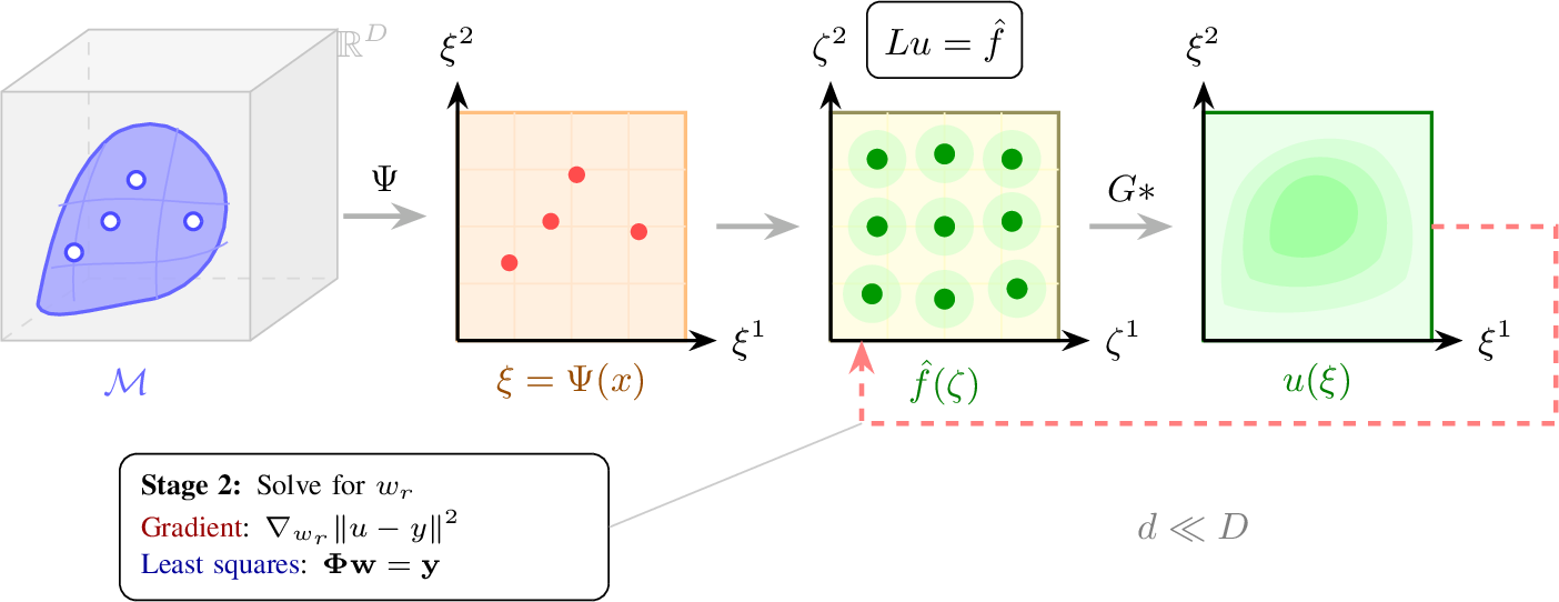
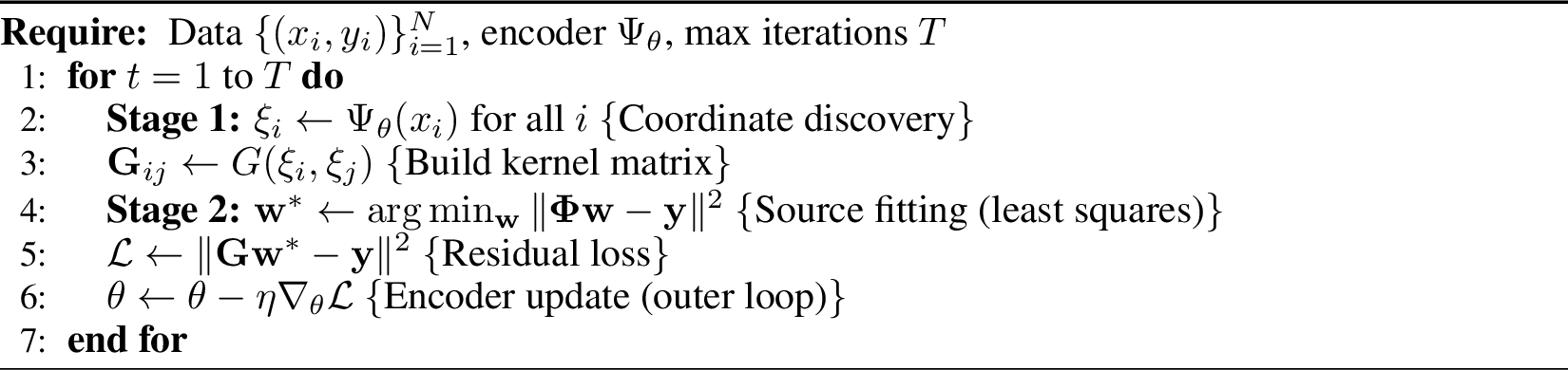
The central contribution of this paper is a two-stage algorithm that separates coordinate discovery from source fitting (Figure 1):
Stage 1 (Coordinate Discovery): An encoder \(\Psi: \mathbb{R}^D \to \mathbb{R}^d\) discovers a coordinate chart where the source \(f\) and operator \(L\) decompose as low-rank tensors such that solving the EDP is essentially equivalent to \(d\) 1D integrals.
Stage 2 (Source Fitting): Given coordinates from Stage 1, solve for source weights and kernel scales. The factorized integral (Eq. 3 ) is linear, making this a nearly convex problem with only \(O(KR)\) parameters where \(K\) are the number of kernel components and \(R\) is the rank of the source tensor, which is fast and interpretable.
Because IGL requires a learned chart where the source admits low-rank tensor factorization, it is not a drop-in replacement for generic deep learning models. Rather, it is best used as a geometric regularizer or parallel head alongside a flexible model. We demonstrate empirically that:
two-stage training prevents dimensional collapse and discovers intrinsic dimension automatically via learnable gates;
the two-stage training also drives a sharp sample-efficiency phase transition;
operator superposition (Gabor wavelets, multi-scale kernels) overcomes the smoothness bias of single-kernel methods;
ResIGL, an MLP augmented with an IGL branch, preserves manifold topology while the MLP captures sharp features;
IGL acts as an effective latent-space regularizer on MNIST, achieving automatic dimension discovery with near-optimal classification.
2 Related Work↩︎
2.0.0.1 Physics-Informed Neural Networks.
PINNs [4] learn solutions \(u\) and enforce physics via residual \(\|Lu_\theta - f\|^2\). IGL approaches this from the integral side (Section 3).
2.0.0.2 Kolmogorov-Arnold Networks.
KANs [5] represent functions as compositions of univariate functions: \(u(x) = \sum_q \Phi_q(\sum_p \phi_{q,p}(x_p))\). IGL uses a different mechanism: kernel convolutions with tensor-factored structure. Both share the philosophy of decomposition into univariate components; KANs use function composition while IGL uses integral convolution. Crucially, IGL’s two-stage structure separates coordinate discovery (Stage 1) from univariate fitting (Stage 2), whereas KANs optimize both simultaneously.
2.0.0.3 Tensor Decompositions.
Canonical Polyadic (CP) and Tucker decompositions [6] assume separability in original coordinates. In the PDE context, tensor numerical methods solve forward problems efficiently: given a known operator \(L\), known source \(f\), and fixed coordinates, compute \(u = G*f\) via low-rank Kronecker products [7], [8]. IGL inverts this pipeline: the operator, source, and coordinates are all unknown and learned from data. The Fubini factorization (Eq. 3 ) uses the same tensor algebra but applied to an inverse problem: fitting observations rather than solving a given PDE.
2.0.0.4 Additive Models and GAMs.
Generalized Additive Models represent \(u = \sum_j u_j(x_j)\). IGL generalizes GAMs: additive models are the special case with tensor rank \(K=1\). \(K > 1\) enables representation of non-additive functions (products, radial, XOR).
2.0.0.5 Geometric Deep Learning.
Spectral networks [9] and Graph Neural Diffusion (GRAND) [10] learn on manifolds via spectral operators. IGL shares the PDE-on-manifold philosophy but differs in learning the source term rather than the solution directly, and in using tensor decomposition for scalability.
2.0.0.6 Operator Learning.
Neural operator methods—DeepONet [11] and Fourier Neural Operator [12]—learn solution operators \(f \mapsto u\) as mappings between function spaces, while [13] learn Green’s functions directly from PDE solution data. IGL differs in that the operator \(L\) is chosen as an inductive bias (not learned from PDE data), the source \(f\) is the primary learned object (not the operator), and tensor decomposition provides explicit factorization. IGL is complementary: it uses PDE structure as an architectural prior for supervised learning, whereas operator learning approximates PDE solvers.
2.0.0.7 Sufficient Dimension Reduction.
Neural Eigenfunctions [14] learn spectral decompositions of a fixed kernel operator to discover structured representations; sufficient dimension reduction (SDR) methods find linear subspaces capturing \(Y \mid X\). IGL discovers nonlinear coordinates where the source term admits tensor decomposition, enabling physics-structured fitting via integration rather than regression in a spectral or linear subspace.
| Method | Coords | Principle | Complexity |
|---|---|---|---|
| MLPs | Implicit | Composition | \(O(DW^2)\) |
| PINNs | No | Differentiation | \(O(DW^2)\) |
| Kernels | No | Integration | \(O(N^2)\) |
| KANs | Grids | Composition | \(O(DG)\) |
| Neural Ops | Given | Integration | \(O(N_\text{modes}^d)\) |
| IGL | Learned | Integration | \(O(DW^2{+}KRd)\) |
3 The IGL Framework↩︎
3.1 Problem and Method Overview↩︎
We consider learning a target function \(u: \mathcal{M} \to \mathbb{R}^C\) from observations \(\{(x^{(n)}, y^{(n)})\}_{n=1}^N\), where \(\mathcal{M} \subset [0,1]^D\) is a manifold with \(\dim(\mathcal{M}) = d \ll D\). We model the target as a solution to a linear PDE \(Lu = f\), where \(L\) is a linear differential operator and \(f\) is a learned source term: \[u(\xi) = (L^{-1}f)(\xi) = \int_{\mathcal{M}} G(\xi, \zeta) f(\zeta) \, d\zeta\] where \(G\) is the Green’s function of \(L\), used in its free-space form on \(\Omega = \Psi(\mathcal{M})\).
IGL comprises three components (Figure 1), optimized via a two-stage algorithm (Appendix 8.1): an encoder \(\Psi: \mathbb{R}^D \to \mathbb{R}^d\) mapping data to intrinsic coordinates, a tensor source \(\hat{f}(\zeta) = \sum_{r=1}^R w_r \prod_{j=1}^d \phi_{r,j}(\zeta^j)\) with rank-\(R\) CP decomposition, and a Green’s kernel \(G(\xi,\zeta) \approx \sum_{k=1}^K \gamma_k \prod_{j=1}^d G_{k,j}(\xi^j, \zeta^j)\) with rank-\(K\) approximation. The tensor structure enables efficient integration via Fubini’s theorem, reducing a \(d\)-dimensional integral to \(d\) one-dimensional integrals.
The complete pipeline is: \[\begin{align} \xi &= \Psi(x) \in \mathbb{R}^d\\ u(\xi) &= \sum_{k,r} \gamma_k w_r \prod_{j=1}^d I_{k,r,j}(\xi^j) \;+\; \sum_{|\beta| \le p} c_\beta \prod_{j=1}^d (\xi^j)^{\beta_j}\\ \min_{\theta}\; &\sum_{n=1}^N \ell\bigl(u_\theta(x^{(n)}),\, y^{(n)}\bigr) + \lambda \sum_{r=1}^{R_{\max}} \left\| w_r \boldsymbol{\gamma} \right\|_2\\ \underbrace{w^* = \arg\min_w \|\Phi w - y\|^2}_{\text{Stage 2 (inner, linear)}} &\qquad \underbrace{\min_{\theta_\Psi}\; \|y - \Phi(\theta_\Psi)\, w^*(\theta_\Psi)\|^2}_{\text{Stage 1 (outer, encoder)}} \end{align}\] Each component is detailed below; the full Variable Projection algorithm is given in Appendix 8.1.
3.1.0.1 Optimization and parameter split.
The complete parameter set splits across two stages: Stage 1 (outer, nonlinear) optimizes \(\theta_1 = \{\theta_\Psi,\, \{g_j\}_j,\, \{\mu_{r,j}, \rho_r\}_{r,j},\, \{\sigma_{k,j}\}_{k,j}\}\); Stage 2 (inner, linear) solves for \(\theta_2 = \{\{w_r\}_r,\, \{\gamma_k\}_k,\, \{c_\beta\}_{|\beta| \le p}\}\). The Group Lasso penalty in the loss induces sparsity at the level of entire tensor components, and is combined with gating: each coordinate \(\xi^j\) is multiplied by a learnable gate \(g_j \in [0,1]\), so the penalty drives inactive gates to zero, discovering the intrinsic dimension automatically. Joint optimization of all parameters is prone to dimensional collapse; the two-stage split prevents this by solving Stage 2 to optimality at each outer step, so the encoder gradient reflects only how well the coordinates serve the fitting problem (Appendix 8.1).
3.2 The Factorized Integral↩︎
IGL factorizes a \(d\)-dimensional integral into \(d\) independent 1D integrals via tensor decomposition of both source and Green’s function.
3.2.0.1 Rank-\(R\) tensor source.
We parametrize the source as a CP decomposition: \[\hat{f}(\zeta) = \sum_{r=1}^R w_r \prod_{j=1}^d \phi_{r,j}(\zeta^j) \label{eq:tensor95source95def}\tag{1}\] where \(\phi_{r,j}\) are univariate basis functions and in practice \(\zeta\) are coordinates on the intrinsic manifold obtained by an encoder \(\Psi: \mathbb{R}^D \to \mathbb{R}^d\).
3.2.0.2 Rank-\(K\) Green’s approximation.
We approximate the Green’s function as: \[G(\xi, \zeta) \approx \sum_{k=1}^K \gamma_k \prod_{j=1}^d G_{k,j}(\xi^j, \zeta^j) \label{eq:tensor95green95def}\tag{2}\]
The key result is that tensor decomposition enables factorization of the \(d\)-dimensional integral: \[\boxed{u(\xi) = \sum_{k=1}^K \sum_{r=1}^R \gamma_k w_r \prod_{j=1}^d I_{k,r,j}(\xi^j)} \label{eq:master}\tag{3}\] where \(I_{k,r,j}\) denotes a 1D integral that can take two forms:
Spatial: \(I_{k,r,j}(\xi^j) = \int G_{k,j}(\xi^j, \zeta^j) \, \phi_{r,j}(\zeta^j) \, d\zeta^j\) (convolution with Green’s kernel)
Spectral: \(I_{k,r,j}(\xi^j) = \sum_{n_j} \varphi_{n_j}^{(j)}(\xi^j) \, \hat{\phi}_{r,n_j}^{(j)} \, e^{-\alpha_k \lambda_{n_j}^{(j)}}\) (eigenfunction expansion)
The spectral form arises from expanding Green’s function in eigenmodes; the exponential sum trick [15], [16] converts additive eigenvalues to products (Appendix 8.2). Proofs appear in Appendix 6.1 and 6.2.
On curved manifolds, the metric volume element \(\sqrt{|g|}\) would break this factorization; IGL circumvents this via a compensated source (Appendix 6.3).
3.2.0.3 Complete solution.
Eq. 3 computes the particular solution \(G * \hat{f}\). The complete solution to \(Lu = f\) is \(u = G*f + u_h\) where \(Lu_h = 0\). Null-space functions (e.g. constants and linear trends for the Laplacian, plane waves for Helmholtz) require high tensor rank to approximate via \(G*\hat{f}\) alone. Following standard RBF augmentation [17], [18], we include polynomials up to degree \(p\): \[u(\xi) = \sum_{k,r} \gamma_k w_r \prod_{j=1}^d I_{k,r,j}(\xi^j) \;+\; \sum_{|\beta| \le p} c_\beta \prod_{j=1}^d (\xi^j)^{\beta_j} \label{eq:augmented95master}\tag{4}\] Each monomial \(\prod_j (\xi^j)^{\beta_j}\) is already a rank-1 tensor, adding only \(\binom{d+p}{p}\) coefficients (\(d{+}1\) for \(p{=}1\)) without breaking factorization or changing asymptotic complexity. In the spectral formulation, the analogous fix includes the zero-eigenvalue modes \(\{\varphi_n : \lambda_n = 0\}\) as free parameters (Appendix 8.2). Operators with a spectral gap (\(\lambda_{\min} > 0\)), such as Helmholtz or the harmonic oscillator, have trivial null spaces and require no augmentation.
4 Experiments↩︎
We organize experiments around three questions. Does the two-stage split help? Exp. 1 compares topology preservation against joint training; Exp. 2 locates the sample-efficiency phase transition. Do the framework’s properties hold in practice? Exp. 3 confirms \(O(KRd)\) scaling, Exp. 4 shows Gabor operators overcome smoothness bias, and Exp. 5 checks that ResIGL preserves manifold geometry. Finally, Exps. 6–7 test the full pipeline on a high-dimensional synthetic problem and on MNIST.
4.0.0.1 Exp. 1: Topology Preservation via Two-Stage Training.
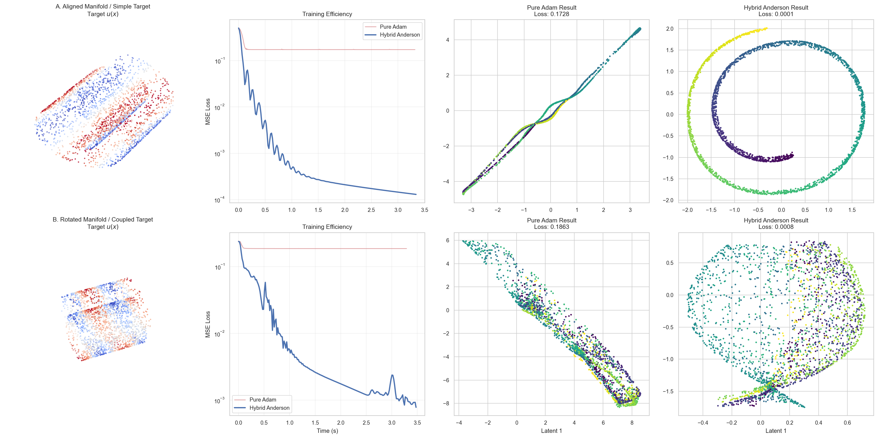
We compare joint optimization versus two-stage training on the Swiss Roll (Figure 2). Two-stage training separates coordinate discovery from fitting, preventing dimensional collapse: by solving Stage 2 to optimality, the encoder is forced to unfold the manifold rather than exploiting source capacity shortcuts. In the rotated setting, joint training fails completely while two-stage training acts as a blind source separator, identifying intrinsic coordinates despite mixing.
4.0.0.2 Exp. 2: Sample Efficiency.
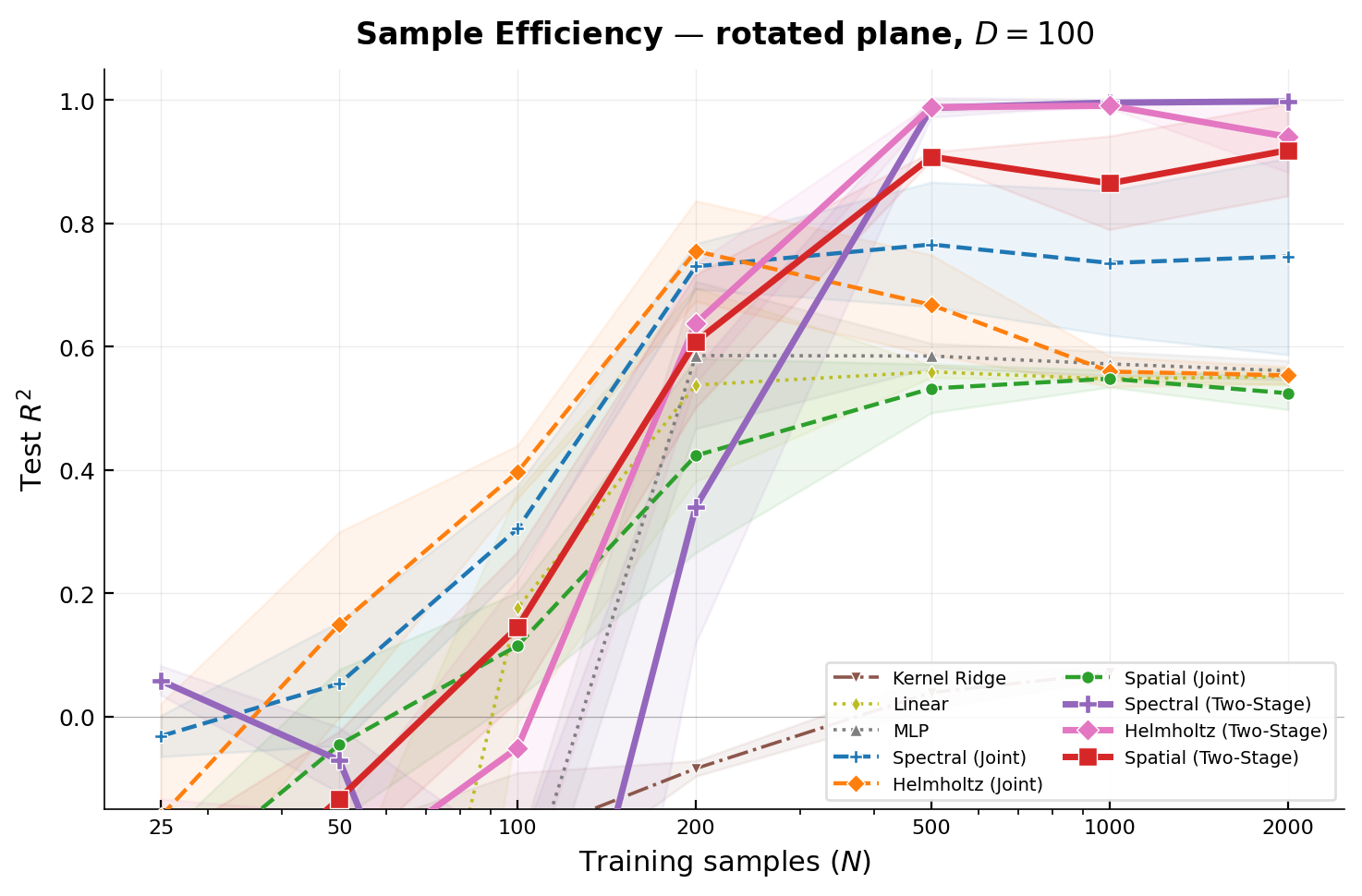
We construct a controlled regression problem: a 2D plane in \(\mathbb{R}^{100}\) via random rotation, with a non-separable multi-frequency target. All methods share the same encoder and differ only in the regression head (three Green’s kernels \(\times\) joint/two-stage, plus MLP and kernel ridge baselines; 3 seeds each). Figure 3 reveals a sharp phase transition: between \(N{=}200\) and \(N{=}500\), all two-stage kernels exceed \(R^2 > 0.9\) while jointly-trained counterparts plateau between \(0.53\) and \(0.77\). At \(N{=}2000\), Spectral (Two-Stage) reaches \(R^2 = 0.998\) vs.\({\approx}0.55\) for all joint methods. The gap arises from optimization structure alone, as architectures are identical: the exact inner solve ensures outer gradients reflect purely coordinate quality.
4.0.0.3 Exp. 3: Scalability.
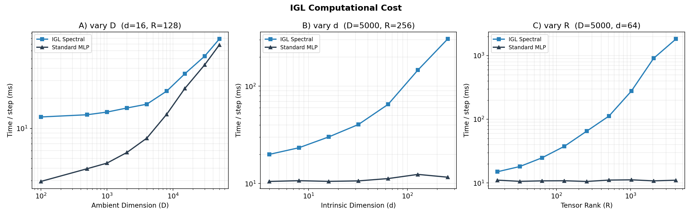
Figure 4 validates the cost decomposition: the encoder (here a 2-layer MLP, but any architecture applies) dominates at all tested scales, while Stage 2 adds overhead that is linear in \(d\) and \(R\) but negligible in absolute terms. For the practical regime \(K \!\leq\! 10\), \(R \!\leq\! 64\), \(d \!\leq\! 10\), Stage 2 overhead is negligible; Experiment 7 confirms this on real data.
| Operator | MSE (\(\times 10^{-6}\)) | \(d_\text{eff}\) | ||
|---|---|---|---|---|
| 2-3 (lr)4-5 | \(R{=}32\) | \(R{=}128\) | \(R{=}32\) | \(R{=}128\) |
| Gaussian | \(4.8 \pm 4.1\) | \(1.7 \pm 0.2\) | 4 | 3 |
| Helmholtz | \(18.6 \pm 3.3\) | \(9.6 \pm 0.6\) | 3 | 3 |
| Cauchy | \(5.6 \pm 5.0\) | \(2.0 \pm 0.3\) | 3 | 3 |
All operators recover \(d_\text{eff} = 3\)–\(4\) (true \(d\) plus embedding curvature overhead) regardless of rank \(R\), while MSE improves by \(2\)–\(5{\times}\) from \(R{=}32\) to \(R{=}128\) (Table 2). Operator choice affects approximation quality but not structural discovery, at least on simple manifolds.
4.0.0.4 Exp. 4: Expressivity — Gabor Wavelets and Superposition.
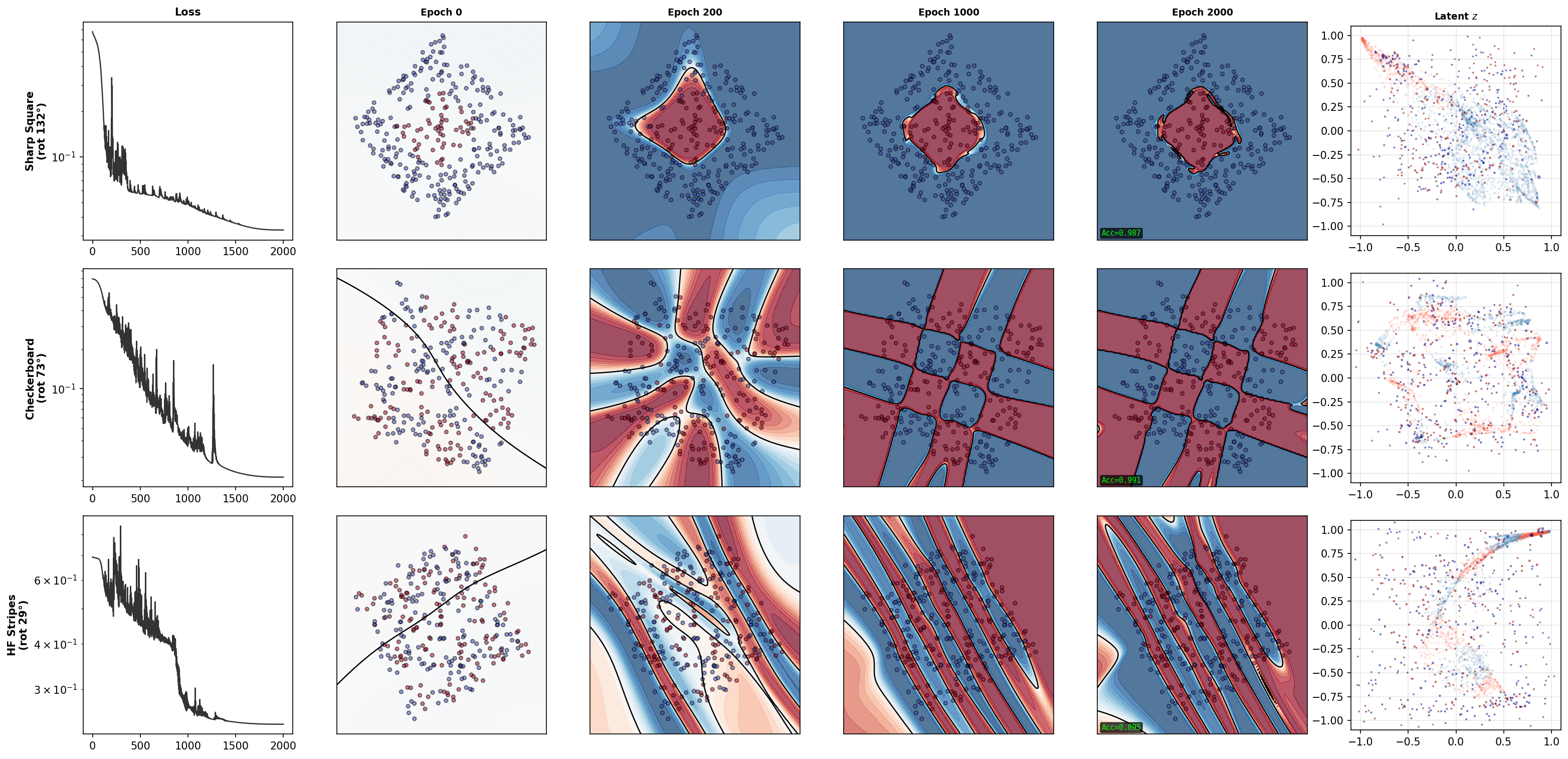
Gabor wavelets overcome the smoothness bias common to Green’s function methods (Figure 5). Stage 1 discovers coordinates aligned with the pattern geometry despite arbitrary rotations; Stage 2’s Gabor basis then captures sharp boundaries via localized oscillatory components.
4.0.0.5 Exp. 5: ResIGL — IGL as Geometric Regularizer.
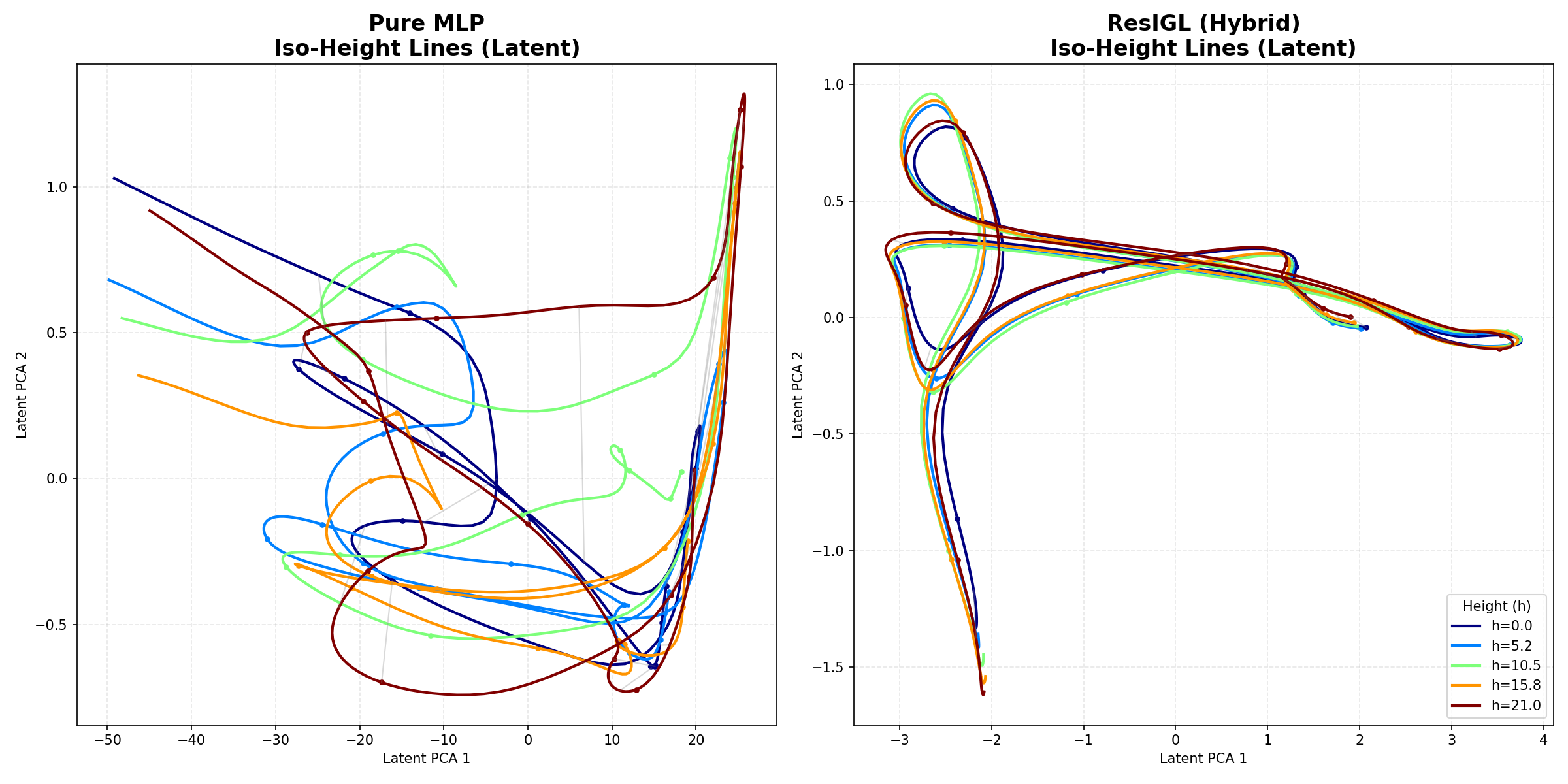
In this experiment, we model the target as a decomposition: \[u(x) = \underbrace{\int G(\xi, \zeta)f(\zeta) d\zeta}_{\text{IGL: Topology \& Global Trend}} + \underbrace{\mathcal{M}(\xi)}_{\text{MLP: Sharp Residuals}}\] Figure 6 shows that pure MLP collapses iso-height curves, while ResIGL maintains stratification. The IGL branch acts as a geometric regularizer: because Stage 2 has few parameters (\(O(KR)\)) and integration is a smoothing operation, the IGL output is inherently smooth and topology-preserving. The MLP residual then captures sharp features without destroying the underlying geometry.
4.0.0.6 Exp. 6: Coordinate Discovery and Regression.
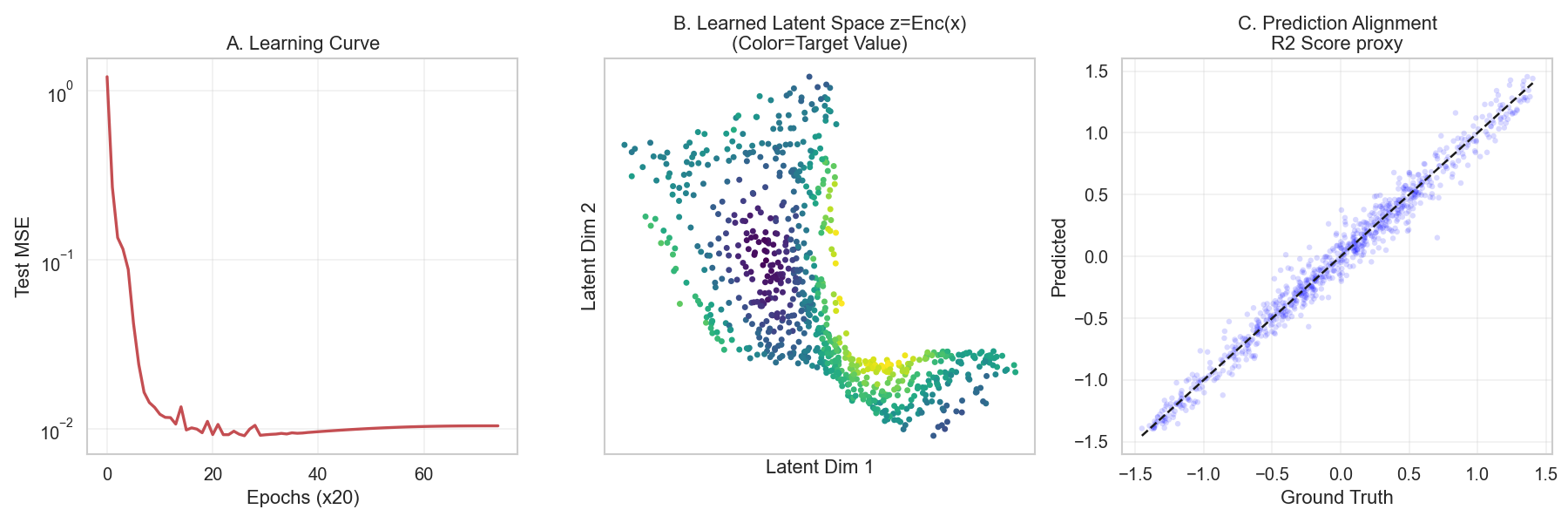
Figure 7 shows the full two-stage pipeline: Stage 1 discovers a 2D coordinate chart from a randomly rotated embedding in \(\mathbb{R}^{100}\), and Stage 2 achieves MSE \(< 0.01\) on a non-separable target.
4.0.0.7 Exp. 7: Latent Space Regularization on MNIST.
| Method | MSE \(\downarrow\) | Lin.Probe \(\uparrow\) | Silhouette \(\uparrow\) | Smooth \(\downarrow\) | Dims |
|---|---|---|---|---|---|
| AE-only | 0.0021 | 0.918 | 0.060 | 0.139 | 64 |
| AE+KL | 0.0073 | 0.933 | 0.042 | 0.156 | 64 |
| AE+Contrastive | 0.0023 | 0.992 | 0.744 | 0.172 | 64 |
| AE+IGL(Two-stage) | 0.0036 | 0.991 | 0.630 | 0.122 | 12 |
| AE+IGL(Joint) | 0.0025 | 0.990 | 0.470 | 0.123 | 9 |
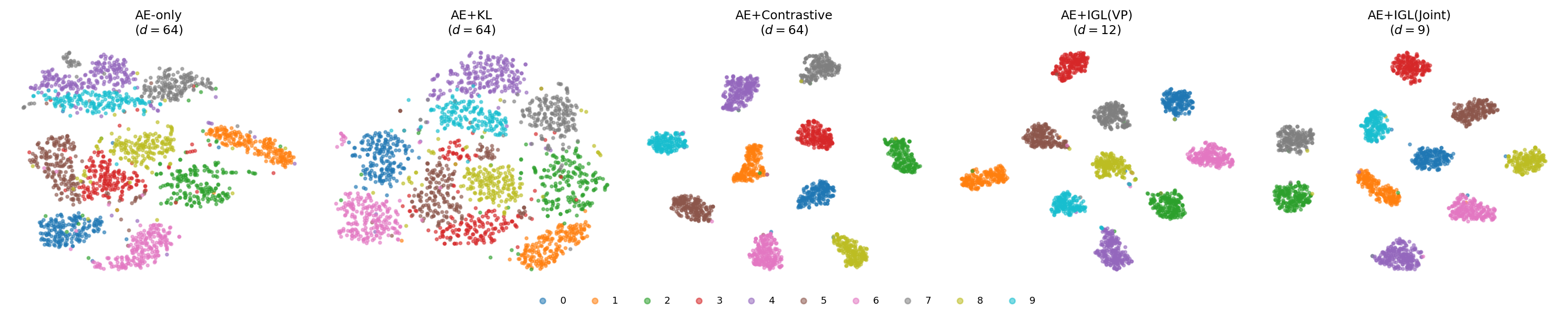
We evaluate IGL as a topological regularizer for autoencoder latent spaces on MNIST (10 classes, 20 k samples). A shared CNN encoder maps \(28 \times 28\) images to a 64-dimensional latent space with learnable gates; the latent code \(\mathbf{z}\) feeds two heads. A CNN decoder reconstructs the input: \[\hat{\mathbf{x}} = h_\phi(\mathbf{z}), \qquad \mathcal{L}_{\mathrm{recon}} = \| \mathbf{x} - \hat{\mathbf{x}} \|^2 + \lambda_e \, \mathcal{L}_{\mathrm{edge}}(\mathbf{x}, \hat{\mathbf{x}}). \label{eq:decoder}\tag{5}\] The IGL classification head computes a multi-scale Green’s integral via the factorized integral (Eq. 3 ) with \(R=128\) RBF anchors at 4 length scales and predicts 10-class logits.
Table 3 and Figure 8 summarize the results. AE+IGL(Two-stage) uniquely combines near-optimal linear probe accuracy (0.991), strong silhouette score (0.630), best label smoothness (0.122), and automatic dimension discovery (12 of 64 gates active). The mechanism follows directly from the two-stage procedure (§3): by solving Stage 2 to optimality at each step, the encoder is forced to produce geometrically discriminative coordinates rather than collapsing classes. AE+IGL(Joint) achieves comparable classification accuracy but lower silhouette (0.470), confirming the hypothesis of §3 that co-adaptation allows the encoder to find degenerate solutions that collapse classes into point clusters. AE+Contrastive achieves the best silhouette (0.744) but retains all 64 dimensions, performs no structure discovery, and exhibits the worst label smoothness (0.172). The discovered dimension of 12 is consistent with the intrinsic dimension of MNIST, which has been estimated to be around 10–15 in prior work [1], [2].
5 Discussion and Conclusion↩︎
5.0.0.1 Summary.
IGL separates coordinate discovery from source fitting via a two-stage algorithm. Stage 2 adds only \(O(KRd)\) cost on top of any encoder, where \(K = O(\log\varepsilon^{-1})\) is dimension-independent. The operator \(\times\) rank ablation (Table 2) confirms structural discovery is robust across 100 configurations, and IGL’s gating mechanism discovers 12 of 64 active dimensions on MNIST (Table 3), consistent with prior estimates.
5.0.0.2 Conclusion.
IGL reframes supervised learning on manifolds as an inverse PDE problem: learn a source term, integrate against a Green’s kernel. Tensor decomposition with metric compensation collapses the resulting high-dimensional integral to \(O(KRd)\) cost, linear in intrinsic dimension, while the two-stage algorithm keeps source fitting near-convex. Experiments confirm topology preservation, scalability, and expressivity gains from operator superposition on synthetic manifolds and on MNIST.
5.0.0.3 Future work.
Scaling IGL to larger benchmarks (CIFAR-10, ImageNet) and to manifolds of higher intrinsic dimension is the most immediate next step. The two-stage structure also invites meta-learning: amortize Stage 1 across a task distribution, adapting only the lightweight Stage 2 per problem.
6 Proofs↩︎
6.1 Proof of the Factorized Integral (Eq. 3 )↩︎
We prove the factorized integral in its most general (compensated) form; setting \(\sqrt{|g|} = 1\) recovers the flat-space case.
Proof. Substituting the tensor decompositions into the compensated integral: \[\begin{align} \tilde{u}(\xi) &= \int_\Omega \tilde{G}(\xi, \zeta) \cdot \hat{f}(\zeta) \, d\zeta \\ &= \int \left[\sum_{k=1}^K \gamma_k \prod_{j=1}^d G_{k,j}(\xi^j, \zeta^j)\right] \left[\sum_{r=1}^R w_r \prod_{j=1}^d \phi_{r,j}(\zeta^j)\right] d\zeta \\ &= \sum_{k,r} \gamma_k w_r \int \prod_{j=1}^d \left[G_{k,j}(\xi^j, \zeta^j) \phi_{r,j}(\zeta^j)\right] d\zeta^1 \cdots d\zeta^d \\ &= \sum_{k,r} \gamma_k w_r \prod_{j=1}^d \underbrace{\int G_{k,j}(\xi^j, \zeta^j) \phi_{r,j}(\zeta^j) \, d\zeta^j}_{I_{k,r,j}(\xi^j)} \quad \text{(Fubini)} \end{align}\] The key step is Fubini’s theorem in the last line, which is valid because the integrand is a product of functions, each depending on a single integration variable \(\zeta^j\). When the source is compensated (\(\hat{f} = \tilde{f} \cdot \sqrt{|g|}\)), the basis functions \(\phi_{r,j}\) implicitly absorb the metric factor; the algebraic structure is identical. ◻
6.2 Proof of the Spectral Factorized Integral (Eq. 3 , spectral form)↩︎
Proof. Substituting the factorized Green’s function (with exponential sum approximation) and tensor source into the convolution integral, then applying Fubini’s theorem to separate the \(d\)-dimensional sum/integral into \(d\) independent 1D operations.
Specifically, starting from the spectral representation: \[G(\xi, \zeta) = \sum_{\mathbf{n}} \frac{\prod_{j=1}^d \varphi_{n_j}^{(j)}(\xi^j) \varphi_{n_j}^{(j)}(\zeta^j)}{\sum_{j=1}^d \lambda_{n_j}^{(j)}}\] and applying the exponential sum approximation \(1/\lambda \approx \sum_k \gamma_k e^{-\alpha_k \lambda}\), we obtain: \[\begin{align} u(\xi) &= \sum_{\mathbf{n}} \frac{\hat{f}_{\mathbf{n}}}{\lambda_{\mathbf{n}}} \varphi_{\mathbf{n}}(\xi) \\ &\approx \sum_k \gamma_k \sum_{\mathbf{n}} e^{-\alpha_k \sum_j \lambda_{n_j}^{(j)}} \hat{f}_{\mathbf{n}} \prod_j \varphi_{n_j}^{(j)}(\xi^j) \\ &= \sum_k \gamma_k \sum_{\mathbf{n}} \prod_j e^{-\alpha_k \lambda_{n_j}^{(j)}} \hat{f}_{\mathbf{n}} \prod_j \varphi_{n_j}^{(j)}(\xi^j) \end{align}\] With the tensor source \(\hat{f}(\zeta) = \sum_r w_r \prod_j \phi_{r,j}(\zeta^j)\), we have \(\hat{f}_{\mathbf{n}} = \sum_r w_r \prod_j \hat{\phi}_{r,n_j}^{(j)}\), and the result follows by regrouping. ◻
6.3 Proof of the Separability Barrier↩︎
Proof. Write the integral with separable \(G\): \[\tilde{u}(\xi) = \int \prod_j G_j(\xi^j, \zeta^j) \cdot \tilde{f}(\zeta) \cdot \sqrt{|g(\zeta)|} \, d\zeta^1 \cdots d\zeta^d\] Fubini’s theorem allows factorization into independent 1D integrals if and only if the integrand can be written as a product of functions, each depending on a single \(\zeta^j\).
For the “if” direction: If \(\sqrt{|g(\zeta)|} = \prod_j \chi_j(\zeta^j)\) and \(\tilde{f}(\zeta) = \sum_r w_r \prod_j \phi_{r,j}(\zeta^j)\), then: \[\begin{align} \tilde{u}(\xi) &= \int \prod_j G_j(\xi^j, \zeta^j) \cdot \sum_r w_r \prod_j \phi_{r,j}(\zeta^j) \cdot \prod_j \chi_j(\zeta^j) \, d\zeta \\ &= \sum_r w_r \int \prod_j \left[G_j(\xi^j, \zeta^j) \phi_{r,j}(\zeta^j) \chi_j(\zeta^j)\right] d\zeta \\ &= \sum_r w_r \prod_j \int G_j(\xi^j, \zeta^j) \phi_{r,j}(\zeta^j) \chi_j(\zeta^j) \, d\zeta^j \end{align}\]
For the “only if” direction: If \(\sqrt{|g|}\) mixes coordinates (i.e., cannot be written as a product), then for any fixed \(\tilde{f}\), the integrand \(\prod_j G_j \cdot \tilde{f} \cdot \sqrt{|g|}\) cannot be factored. The cross-terms in \(\sqrt{|g|}\) create dependencies between coordinates that persist through the integration. ◻
7 Theoretical Analysis↩︎
7.1 Low-Rank Justification↩︎
We provide an analysis of when and why low-rank tensor approximations suffice in the IGL framework. The analysis splits into two parts: the Green’s function \(G\) (rigorous for most operators) and the source \(\hat{f}\) (conditional on the encoder).
7.1.0.1 The Green’s function: rigorous low-rank bounds.
For asymptotically smooth kernels, low-rank separable approximations are well-established [7], [16].
The key mechanism is the exponential sum trick: functions like \(1/r\) can be approximated by sums of Gaussians: \[\frac{1}{r} \approx \sum_{k=1}^K \gamma_k e^{-\alpha_k r^2}\] Since a high-dimensional Gaussian factors exactly, the rank \(K\) required to achieve error \(\varepsilon\) scales as \(O(\log(1/\varepsilon))\), independent of dimension, provided \(\lambda_{\min}\) is bounded away from zero. This property is true for elliptic and parabolic operators. When \(\lambda_{\min} \to 0\) (e.g., the free-space Laplacian), \(K\) degrades to \(O(\log(1/\varepsilon) \cdot \log(\lambda_{\max}/\lambda_{\min}))\); the polynomial augmentation (Eq. 4 ) handles these near-null modes directly. For non asymptotically smooth kernels such as high-frequency Helmholtz equation, we can vastly mitigate the problem using a proper basis such as plane waves or Bessel functions and empirical results confirm this; see Figure 7 for validation on high-frequency targets.
7.1.0.2 The source term: coordinate-dependent.
The hypothesis that the source \(\hat{f}\) admits low-rank approximation is more nuanced because the tensor rank is not invariant under coordinate changes:
A radial function \(f(r) = e^{-r^2}\) is rank-1 in polar coordinates
The same function in Cartesian coordinates, \(f(\sqrt{x^2+y^2})\), may require many terms to approximate
This coordinate dependency is precisely why the encoder \(\Psi\) is essential. Standard smoothness (Sobolev regularity) is insufficient to guarantee low tensor rank in high dimensions. However, functions with bounded mixed derivatives (also called “mixed regularity”) do admit efficient tensor approximations [8].
7.1.0.3 Bounded mixed derivatives
The approximation-theoretic foundation for efficient tensor decompositions rests on bounded mixed derivatives. A function \(f: [0,1]^d \to \mathbb{R}\) has bounded mixed derivatives of order \(r\) if: \[\left\| \frac{\partial^{|\alpha|} f}{\partial x_1^{\alpha_1} \cdots \partial x_d^{\alpha_d}} \right\|_\infty \le C \quad \text{for all } \alpha \text{ with } \max_j \alpha_j \le r\] The crucial distinction from standard smoothness is:
| Smoothness Type | Constraint | Approximation Error |
|---|---|---|
| Standard (Sobolev \(H^r\)) | \(\sum_j \alpha_j \le r\) | \(O(N^{-r/d})\) |
| Mixed (Korobov \(H^r_{\text{mix}}\)) | \(\max_j \alpha_j \le r\) | \(O(N^{-r} (\log N)^{d-1})\) |
For standard smoothness, the exponent \(-r/d\) degrades with dimension. For mixed smoothness, the dimension appears only in the logarithmic factor, making it scalable with \(d\). This is why tensor product approximations (Eq. 1 ) achieve tractable complexity in high dimensions.
Intuitively, mixed smoothness controls variable interactions: \(\partial^2 f / \partial x \partial y\) measures how the slope in \(x\) changes as you move in \(y\). Functions with controlled interactions—like \(f(x,y) = \sin(x)\sin(y)\)—have high mixed smoothness. Functions with strongly coupled variables—like radial functions \(f(\|x\|)\)—do not.
7.1.0.4 The encoder as a coordinate search.
Bounded mixed derivatives are coordinate-dependent. A function may have excellent mixed smoothness in one coordinate system but poor mixed smoothness in another for the same reason the tensor rank depends on coordinates. The encoder \(\Psi\) reverses this process: it searches for the diagonalizing coordinates where the target function has bounded mixed derivatives. This is the theoretical justification for why learned coordinates enable efficient tensor decomposition. The optimization landscape favors coordinates where the source factorizes—precisely those where mixed smoothness holds.
7.1.0.5 Empirical enforcement of mixed smoothness.
The theoretical guarantee that the encoder finds good coordinates can be empirically reinforced through the rank-sparsity regularization (Section 3). The Group Lasso penalty on tensor weights flows through both the weights and the encoder \(\Psi\). When coordinates have poor mixed smoothness, more tensor terms are required to fit the data; by penalizing active terms, we incentivize the encoder to discover coordinates where fewer ranks suffice.
7.1.0.6 Differentiation preserves rank.
A potential concern is that applying \(L\) to a low-rank tensor might increase rank. For separable operators \(L = \sum_j L_j\), this is not the case: \[L\hat{f} = \sum_r w_r \sum_j (L_j \phi_{r,j}) \prod_{i \neq j} \phi_{r,i}\] which has rank at most \(Rd\). Differentiation is rank-friendly in tensor formats.
7.1.0.7 Effective rank.
The effective rank \(R\) of the learned source is controlled by the intrinsic complexity of the target on the manifold, not the ambient dimension \(D\). For data on a \(d\)-dimensional manifold with \(d \ll D\):
If \(d\) is small (e.g., \(d < 10\)), even polynomial rank growth is tractable
The encoder \(\Psi\) projects to intrinsic coordinates, where the target is simpler
The \(O(|\log\varepsilon|)\) bound for \(G\) is rigorous; for \(\hat{f}\), it is empirically observed
7.1.0.8 Summary.
| Component | Low-Rank Guarantee | Mechanism |
|---|---|---|
| Green’s function \(G\) | Rigorous: \(K = O(\log \varepsilon^{-1})\) | Exponential sum trick |
| Source \(\hat{f}\) | Conditional on coordinates | Joint \((\Psi, \hat{f})\) optimization |
| Metric \(\sqrt{|g|}\) | Absorbed into \(\hat{f}\) | End-to-end learning |
| Effective rank \(R\) | Scales with intrinsic complexity | Low \(d \ll D\) |
7.2 Separability and Compensation↩︎
This section groups three complementary perspectives on separability and the compensation mechanism: classical coordinate theory (Stäckel), geometric interpretation, and operator-level coupling.
7.2.1 Stäckel Separability↩︎
Classical orthogonal coordinate systems (polar, spherical, cylindrical, ellipsoidal, etc.) belong to the Stäckel class: their scale factors \(h_j\) have a specific structure ensuring that \(\sqrt{|g|} = \prod_j h_j\) is automatically separable. Indeed, all classical separable coordinate systems for the Helmholtz equation share this property.
| Coordinates | \(\sqrt{|g|}\) | Separable? |
|---|---|---|
| Cartesian | 1 | ✔ (trivially) |
| Polar (2D) | \(r\) | ✔ (\(= r \times 1\)) |
| Spherical (3D) | \(r^2 \sin\theta\) | ✔ (\(= r^2 \times \sin\theta \times 1\)) |
| Cylindrical (3D) | \(r\) | ✔ (\(= r \times 1 \times 1\)) |
| Learned \(\Psi\) | Arbitrary | \(\times\) (generically) |
However, a learned encoder \(\Psi: \mathbb{R}^D \to \mathbb{R}^d\) does not produce Stäckel coordinates in general. The induced metric \(g_{ij} = \sum_k (\partial\Psi_i/\partial x_k)(\partial\Psi_j/\partial x_k)\) is generically non-diagonal and non-Stäckel. Even if \(\Psi\) were constrained to produce orthogonal coordinates, it would not satisfy the restrictive Stäckel conditions. This is why the compensation mechanism is essential: it enables separability for arbitrary learned coordinate systems, not just the restricted Stäckel class.
7.2.2 Geometric Interpretation↩︎
The compensation has a natural physical interpretation:
| Quantity | Interpretation |
|---|---|
| \(\tilde{f}(\zeta)\) | Physical source density (per unit coordinate volume) |
| \(\sqrt{|g(\zeta)|}\) | Conversion from coordinate to geometric volume |
| \(\hat{f}(\zeta) = \tilde{f} \cdot \sqrt{|g|}\) | Total source strength (geometry-corrected) |
By learning \(\hat{f}\) directly, we learn the total source strength without ever computing the metric explicitly.
Practical Implementation. In practice, we never explicitly compute \(\sqrt{|g|}\):
Parameterize \(\hat{f}\) directly as a rank-\(R\) tensor (Eq. 1 )
Train end-to-end on the task loss
The learned \(\hat{f}\) implicitly absorbs whatever structure is needed
This adds zero computational overhead: the compensation is entirely representational. This is not a problem if we are not interested in preserving the geometric structure of the manifold.
7.2.3 Operator Coupling and Double Compensation↩︎
The preceding analysis focused on the metric volume factor \(\sqrt{|g|}\) in the integral measure. A related but distinct source of non-separability arises from the operator itself.
7.2.3.1 The Laplace-Beltrami decomposition.
On a Riemannian manifold with metric \(g_{ij}\), we can decompose \(\tilde{L}\) as \(\tilde{L} = \tilde{L}_{\text{sep}}+ \tilde{L}_{\text{coup}}\), where:
\(\tilde{L}_{\text{sep}}= \sum_j L_j\) is the separable part, with each \(L_j\) acting only on coordinate \(\xi^j\)
\(\tilde{L}_{\text{coup}}\) contains coupling terms: off-diagonal metric components \(g^{ij}\) (\(i \neq j\)) and cross-derivatives of \(\sqrt{|g|}\)
7.2.3.2 The separable Green’s function.
Let \(G_{\text{sep}}\) denote the Green’s function of \(\tilde{L}_{\text{sep}}\) (satisfying \(\tilde{L}_{\text{sep}}G_{\text{sep}}= \delta\)). By construction, \(G_{\text{sep}}\) factorizes: \(G_{\text{sep}}(\xi, \zeta) = \prod_j G_j(\xi^j, \zeta^j)\).
The true Green’s function \(\tilde{G}\) of the full operator \(\tilde{L}\) is related by: \[\tilde{G} = (\tilde{L}_{\text{sep}}+ \tilde{L}_{\text{coup}})^{-1} = G_{\text{sep}}(I + G_{\text{sep}}\tilde{L}_{\text{coup}})^{-1}\] When \(\tilde{L}_{\text{coup}}\neq 0\), the true \(\tilde{G}\) is not separable—the coupling terms mix coordinates.
7.2.3.3 Why the separable approximation works.
The IGL framework uses separable kernel approximations rather than the true \(\tilde{G}\). This is valid because for any target \(u^*\) in the range of \(G_{\text{sep}}\), setting \(\hat{f} = \tilde{L}_{\text{sep}}u^*\) yields \(G_{\text{sep}}\hat{f} = u^*\) by definition of \(G_{\text{sep}}= \tilde{L}_{\text{sep}}^{-1}\).
Specifically, the required source is: \[\hat{f} = \tilde{L}_{\text{sep}}u^* = (\tilde{L} - \tilde{L}_{\text{coup}}) u^* = f - \tilde{L}_{\text{coup}}u^*\] where \(f = \tilde{L} u^*\) is the “true” source. The learned \(\hat{f}\) implicitly absorbs the correction \(-\tilde{L}_{\text{coup}}u^*\).
7.2.3.4 Double compensation.
When we learn \(\hat{f}\) end-to-end with a separable kernel, the optimization finds whatever compensated source makes \(G_{\text{sep}}\hat{f}\) match the target \(u^*\). This simultaneously compensates for:
The metric volume factor \(\sqrt{|g|}\) in the integral measure
The kernel mismatch from using \(G_{\text{sep}}\) instead of \(\tilde{G}\)
These two compensations differ in their rank cost. Metric absorption \(\hat{f} = \tilde{f} \cdot \sqrt{|g|}\) is exact but incurs a multiplicative cost: \(\mathrm{rank}(\tilde{f} \cdot \sqrt{|g|}) \le \mathrm{rank}(\tilde{f}) \times \mathrm{rank}(\sqrt{|g|})\). The operator correction is additive: the total rank satisfies \(\mathrm{rank}(\hat{f}) \le \mathrm{rank}(\tilde{f} \cdot \sqrt{|g|}) + \mathrm{rank}(\tilde{L}_{\text{coup}}u^*)\). The metric cost is a structural property of the chart, independent of the optimization method, so both joint and two-stage training face it equally. The operator correction, however, is where the two-stage algorithm (Section 3) provides its key advantage: by solving Stage 2 to optimality, the reduced objective’s gradient reflects only how well coordinates serve the fitting problem. This prevents the optimizer from tolerating large \(\|\tilde{L}_{\text{coup}}\|\) and wasting rank budget on the correction, explaining the empirical observation that joint optimization tends to collapse dimensions compared to the two-stage solver.
7.3 Expressivity: Overcoming Smoothness Bias↩︎
A common concern with Green’s function methods is smoothness bias: standard operators like the Laplacian are low-pass filters. We clarify that this is a design choice, not an inherent limitation of the IGL framework.
7.3.0.1 The apparent limitation.
The Laplacian’s Green’s function \(G(z,s) \propto |z-s|\) (1D) or \(\propto \log|z-s|\) (2D) decays slowly. Combined with global Fourier basis \(\sin(n\pi x)\), sharp edges require summing many modes—the Gibbs phenomenon. This creates the impression that \(Lu=f\) is fundamentally limited to smooth functions.
7.3.0.2 Solution 1: Localized bases.
Instead of global modes, use Gabor atoms: \[\phi_r(x) = \underbrace{e^{-\alpha_r(x - \mu_r)^2}}_{\text{Gaussian envelope}} \cdot \underbrace{\cos(\omega_r x + \theta_r)}_{\text{oscillation}}\] These provide: localization via learnable position \(\mu_r\) and scale \(\alpha_r\); texture/edges via frequency \(\omega_r\); and multiscale representation where large \(\alpha\) captures sharp edges and small \(\alpha\) captures broad features. Gabor functions are eigenfunctions of the harmonic oscillator \(L = -\Delta + x^2\), biasing toward localized structures (objects) rather than global fields (heat). Similarly, Mexican hat (DoG) wavelets provide edge detection via center-surround receptive fields.
7.3.0.3 Solution 2: Alternative operators.
Different operators encode different inductive biases:
| Operator | Green’s decay | Null space | Suited for |
|---|---|---|---|
| Laplacian \(-\Delta\) | Polynomial | Harmonic poly. | Smooth, global fields |
| Helmholtz \(-\Delta + \mu^2\) | Exponential \(e^{-\mu|z-s|}\) | Trivial (\(\lambda \geq \mu^2\)) | Localized features, edges |
| Harmonic oscillator \(-\Delta + x^2\) | Gaussian | Trivial (\(\lambda \geq d/2\)) | Objects, Gabor atoms |
| Fractional \((-\Delta)^s\) | Power-law | Constants (\(s < d/2\)) | Long-range correlations |
7.3.0.4 Solution 3: Multi-scale decomposition.
The exponential sum (Eq. 10 ) naturally provides multi-scale: small \(\alpha_k\) preserves high frequencies (fine details), while large \(\alpha_k\) retains only low frequencies (smooth background). Combining \(K\) scales enables representation of both sharp edges and smooth regions within the same framework.
7.3.0.5 Solution 4: Operator superposition.
By linearity of the integral, IGL can combine multiple operators: \(u = \sum_k \gamma_k (G_k * \hat{f})\). Different operators create interference patterns, constructive interference sharpens edges while destructive interference smooths transitions. This is analogous to Fourier synthesis but with physics-informed basis functions. The superposition principle enables combining smooth (Laplacian), localized (Helmholtz), and oscillatory (Gabor) components at linear cost.
Summary: IGL’s expressivity is determined by basis and operator design, not by the framework itself. Sharp features, edges, and textures are achievable with appropriate choices: Gabor/wavelet bases, Helmholtz or harmonic oscillator operators, multi-scale decomposition, and operator superposition.
8 Algorithmic Details↩︎
8.1 Two-Stage Training: Variable Projection↩︎
This section provides the full Variable Projection algorithm for Stage 2 optimization, including the integral formulation.
8.1.0.1 Design matrix and linearity.
For fixed encoder and kernel parameters, define the design matrix \[\Phi_{n,(k,r)} = \gamma_k \prod_{j=1}^d I_{k,r,j}(\xi_n^j) \label{eq:design95matrix}\tag{6}\] so that \(u_n = \sum_{k,r} \Phi_{n,(k,r)} \, w_r + \sum_{|\beta| \le p} c_\beta \prod_j (\xi_n^j)^{\beta_j}\). This is a linear regression problem in the combined weights \((w_r, c_\beta)\), solvable by least squares. Stage 2 involves only \(O(KR + \binom{d+p}{p})\) parameters, orders of magnitude fewer than the encoder, and for moderate sample sizes \(N\) can be solved exactly.
8.1.0.2 Encoder requirements.
The encoder \(\Psi: \mathbb{R}^D \to \mathbb{R}^d\) must find coordinates in which the source admits a low-rank tensor decomposition, the operator is approximately separable, and the metric is absorbed into the compensated source (Appendix 7.2).
8.1.0.3 Reduced objective and the envelope theorem.
Two-stage training solves Stage 2 to optimality at each outer step, yielding the reduced objective: \[\mathcal{L}_{\text{red}}(\theta) = \|y - \Phi(\theta) \, w^*(\theta)\|^2 \label{eq:reduced95obj95app}\tag{7}\] where \(w^*(\theta) = \arg\min_w \|\Phi(\theta)w - y\|^2\). By the envelope theorem, \(\partial\mathcal{L}/\partial w = 0\) at the optimum, so \(\nabla_\theta \mathcal{L}_{\text{red}}\) reflects only how well the coordinates serve the fitting problem. This prevents dimensional collapse: the encoder must discover good coordinates because source capacity is fully exploited at every step. The rank-budget interpretation of this cost is analyzed in Appendix 7.2.3.
8.1.0.4 Parameter summary.
For joint training, all parameters \(\theta = \{\theta_\Psi, \{w_r, \mu_{r,j}\}_{r,j}, \{\gamma_k, \sigma_{k,j}\}_{k,j}\}\) are learned simultaneously. For two-stage training, the kernel structure (\(\Psi\), \(\mu_{r,j}\), \(\gamma_k\), \(\sigma_{k,j}\)) is updated in the outer loop, and only source weights \(\mathbf{w} = \{w_r\}\) are solved in the inner loop via least squares.
8.2 Spectral Formulation Details↩︎
The spectral formulation provides an equivalent view of the IGL framework using eigenfunction expansions rather than Green’s kernels.
8.2.0.1 Modal expansion of the Green’s function.
For a self-adjoint operator \(L\) with eigenfunctions \(\{\varphi_n\}\) and eigenvalues \(\{\lambda_n\}\): \[L\varphi_n = \lambda_n \varphi_n, \quad \langle \varphi_n, \varphi_m \rangle = \delta_{nm}\] The Green’s function admits the spectral representation: \[G(\xi, \zeta) = \sum_{n} \frac{\varphi_n(\xi) \varphi_n(\zeta)}{\lambda_n} \label{eq:spectral95green}\tag{8}\]
Remark 1 (Null-space exclusion). The sum in Eq. 8 runs over modes with \(\lambda_n \neq 0\); zero-eigenvalue modes are excluded since \(1/\lambda_n\) diverges. These constitute \(\ker L\) — e.g., constants and harmonic polynomials for the Laplacian. The complete spectral solution includes them as free parameters: \[u(\xi) = \underbrace{\sum_{n:\,\lambda_n > 0} \frac{\hat{f}_n}{\lambda_n}\,\varphi_n(\xi)}_{\text{particular (what IGL computes)}} \;+\; \underbrace{\sum_{n:\,\lambda_n = 0} c_n\,\varphi_n(\xi)}_{\text{homogeneous}} \label{eq:spectral95complete}\qquad{(1)}\] where \(c_n\) are determined by data fitting. For operators with a spectral gap (\(\lambda_{\min} > 0\)), such as Helmholtz (\(\lambda_n \geq \mu^2\)) or the harmonic oscillator (\(\lambda_n \geq d/2\)), the second sum is empty and \(G * \hat{f}\) is already the complete solution.
8.2.0.2 Tensor product eigenfunctions.
On product domains \(\Omega = \Omega_1 \times \cdots \times \Omega_d\) with separable operators \(L = \sum_j L_j\), the eigenfunctions factor: \[\varphi_{\mathbf{n}}(\xi) = \prod_{j=1}^d \varphi_{n_j}^{(j)}(\xi^j), \quad \text{where } L_j \varphi_{n_j}^{(j)} = \lambda_{n_j}^{(j)} \varphi_{n_j}^{(j)}\] and eigenvalues add: \(\lambda_{\mathbf{n}} = \sum_{j=1}^d \lambda_{n_j}^{(j)}\).
8.2.0.3 The spectral separability barrier.
Substituting the tensor product structure (see Appendix 6.3 for the formal proof): \[G(\xi, \zeta) = \sum_{\mathbf{n}} \frac{\prod_{j=1}^d \varphi_{n_j}^{(j)}(\xi^j) \varphi_{n_j}^{(j)}(\zeta^j)}{\sum_{j=1}^d \lambda_{n_j}^{(j)}} \label{eq:spectral95barrier}\tag{9}\] This additive coupling of eigenvalues blocks factorization.
8.2.0.4 Exponential sum factorization.
The key insight is that \(1/\lambda\) can be written as (see Appendix 6.2 for the spectral proof): \[\frac{1}{\lambda} = \int_0^\infty e^{-\alpha \lambda} \, d\alpha\] Approximating this integral with \(K\) quadrature points \(\{\alpha_k, \gamma_k\}\): \[\frac{1}{\sum_j \lambda_j} \approx \sum_{k=1}^K \gamma_k \exp\left(-\alpha_k \sum_{j=1}^d \lambda_j\right) = \sum_{k=1}^K \gamma_k \prod_{j=1}^d e^{-\alpha_k \lambda_j} \label{eq:exp95sum95trick}\tag{10}\]
8.2.0.5 Conditioning near the null space.
The exponential sum approximation (Eq. 10 ) requires rank \(K = O(\log(1/\varepsilon) \cdot \log(\lambda_{\max}/\lambda_{\min}))\) [15], which diverges as \(\lambda_{\min} \to 0\). Near-zero modes are therefore better handled by the polynomial augmentation (Eq. 4 ) or the spectral free parameters (Eq. ?? ).
8.3 Complexity Analysis↩︎
Encoder architecture \(\Psi\): Stage 1 uses any encoder; we use a 2-layer MLP (\(O(DH)\) per sample) in synthetic experiments and a CNN in the MNIST experiment. The table below isolates the Stage 2 cost, which is the only overhead IGL introduces beyond the encoder.
| Component | Operation | Cost |
|---|---|---|
| Encoder | \(z = \Psi(x)\) | \(O(DH)\) |
| 1D convolutions | \(I_{k,r,j}\) for all \((k,r,j)\) | \(O(KRd)\) |
| Products over \(j\) | \(\prod_j I_{k,r,j}\) for all \((k,r)\) | \(O(KRd)\) |
| Summation | \(\sum_{k,r} \gamma_k w_r (\cdot)\) | \(O(KR)\) |
| Polynomial augm. | \(\sum c_\beta \xi^\beta\) | \(O(\binom{d+p}{p})\) |
| Total | \(O(DH + KRd)\) |
9 Model Details↩︎
9.1 Model Parameters↩︎
@llll@ Component & Symbol & Count & Status
Network weights & \(\theta_\Psi\) & \(O(DH{+}Hd)\) & Learned
Dimension gates & \(g_j \in[0,1]\) & \(d\) & Learned\(^\dagger\)
Anchor positions & \(\mu_{r,j}\) & \(Rd\) & Learned
Source weights & \(w_r\) & \(R\) & Learned
Rank importance & \(\rho_r\) & \(R\) & Learned\(^\ddagger\)
Scale weights & \(\gamma_k\) & \(K\) & Learned
Kernel widths & \(\sigma_{k,j}\) & \(Kd\) & Learned
Polynomial coeff. & \(c_\beta\) & \(\binom{d{+}p}{p}\) & Learned
Scale & bias & \(\alpha,\, b_0\) & \(2\) & Learned
Operator type & \(L\) & — & Hyper.
Max dimension & \(d_{\max}\) & — & Hyper.\(^\dagger\)
Max source rank & \(R_{\max}\) & — & Hyper.\(^\ddagger\)
Green’s rank & \(K\) & — & Hyper.
Null-space degree & \(p\) & — & Hyper.
\(^\dagger\) Group Lasso on \(g_j\) discovers effective dimension \(d_{\mathrm{eff}} \le d_{\max}\).
\(^\ddagger\) Softplus gating on \(\rho_r\) discovers effective rank \(R_{\mathrm{eff}} \le R_{\max}\)
.
9.2 Gauge Symmetry Details↩︎
A crucial feature of learning the encoder \(\Psi\) and source \(\hat{f}\) jointly is the emergence of a gauge symmetry. The integral \(\tilde{u}(\xi) = \int G(\xi, \zeta) \hat{f}(\zeta) \, d\zeta\) is invariant under coordinate transformations if the source transforms inversely. This is analogous to gauge freedom in physics [19] and coordinate-free kernel methods [20].
In our framework, this means the encoder \(\Psi\) is not constrained to learn isometric intrinsic coordinates (preserving true manifold distances), but rather any diffeomorphic chart that simplifies the tensor decomposition of the source. The optimization can discover the specific coordinate chart where the target function \(u\) has the lowest tensor rank—effectively diagonalizing the target function’s complexity.