MILES: Modular Instruction Memory with Learnable Selection for Self-Improving LLM Reasoning
July 08, 2026
1 Introduction↩︎
Large language models (LLMs) demonstrate strong capabilities in complex reasoning and question answering. Recent advances in test-time computation, including chain-of-thought prompting [1], self-consistency [2], and tree search [3], [4], have further improved reasoning performance. In many practical settings, however, problems arrive sequentially rather than in isolation, allowing models to benefit from accumulating reusable experience across related queries [5], [6]. Updating model parameters for every new problem is often costly or infeasible, especially for closed or frozen models [7], [8]. A natural alternative is therefore to maintain an external memory that the LLM consults at test time while its parameters remain frozen [9]–[11]. The central question becomes: how can such a memory be organized, maintained, and reused so that it actually improves reasoning—and continues to improve as more experience accumulates?
Existing memory methods for LLM reasoning store whole-solution templates or strategies and retrieve them per problem [5], [9], [10], which are useful when the new problem closely resembles a seen one, but limited when the new problem has novel structure. Step-level memory [12]–[14] stores smaller units that can be composed flexibly across reasoning steps and across problems with different overall structures, shifting the problem from finding a similar past problem to finding applicable local blocks for the next reasoning step. Among step-level designs, prior work commits to all-text concept/situation pairs [14], pre-formed templates [12], or free-form strategies [6], [11]. A common limitation persists across all of these: selecting which unit to apply at the current step is heuristic, via similarity retrieval or LLM prompting, without optimizing the decision against final-answer correctness. Methods that learn selection from feedback [15]–[17] require fixed action spaces, external labeled corpora, or fine-tuning, which are not compatible with a memory that grows incrementally from the model’s own experience under limited test-time data. Moreover, policies learned offline may not generalize well as test data distribution shifts.
We propose MILES (Modular Instruction Memory with LEarnable Selection for self-improving LLM reasoning), a framework that enables test-time self-improvement by learning to compose reusable step-level reasoning modules from accumulated reasoning experience while keeping the underlying LLM frozen. To support reusable step-level reasoning, MILES stores memory as modular asymmetric pairs of a sub-goal embedding and a corresponding sub-instruction. The sub-goal embedding serves as a retrieval key representing the objective of the next reasoning step, while the sub-instruction is natural-language guidance used to condition generation. Unlike raw CoT traces, MILES stores reusable local reasoning modules. Its asymmetric (embedding, text) representation supports scalable retrieval and incremental memory expansion while preserving flexible instruction generation. To enable learnable memory selection, MILES associates each memory unit with a lightweight selection head and employs a coarse-to-fine retrieval mechanism at inference. A cheap sub-goal similarity-based retrieval stage (Layer 1) followed by selection-head applicability scoring (Layer 2); Layer 1 expands memory and collects dense step-level supervision from confident trajectories, enabling the selection heads to learn reusable memory-selection patterns from reliable reasoning experience. Layer 2 then applies the learned selection heads to guide reasoning on uncertain samples leveraging memory-selection patterns learned from confident trajectories. As a result, MILES turns step-wise memory composition into a learned, correctness-optimized decision under realistic test-time constraints: incremental memory growth, sparse per-item data, no ground-truth labels, and no parameter updates. MILES consistently matches or outperforms prior methods across six reasoning benchmarks while achieving superior accuracy–efficiency tradeoffs. Extensive experiments further validate its effectiveness, robustness, and transferability.
MILES suggests that modular memory composition can serve as a useful mechanism for test-time self-improvement of frozen LLMs. This step-wise memory composition is complementary to prompting and test-time search, providing an additional way to improve reasoning through accumulated experience.
The main contributions of this work are summarized as follows:
The MILES framework for self-improving step-wise memory composition at test time. MILES incrementally builds modular instruction memory from confident reasoning traces and applies the learned memory to uncertain cases, without parameter updates, external supervision, curated training data, or fixed action spaces.
A modular asymmetric memory structure consisting of (sub-goal, sub-instruction) pairs associated with per-item selection heads, naturally enabling a coarse-to-fine selection mechanism that enables both incremental memory expansion and learnable memory composition.
Learnable memory composition. MILES trains lightweight per-item selection heads from rollout outcomes on confident samples, enabling self-supervised and correctness-optimized memory composition under limited test-time data while supporting incremental memory expansion.
Empirical validation. MILES consistently matches or outperforms baseline methods across six reasoning benchmarks and four backbones while achieving superior accuracy–efficiency tradeoffs. Further analyses demonstrate its effectiveness, robustness, and transferability.
2 Related work↩︎
Test-time LLM reasoning. Chain-of-Thought (CoT) prompting [1] and Self-Consistency (SC) [2] improve LLM reasoning through intermediate reasoning and multi-trajectory aggregation. Structured-search methods such as Tree-of-Thought (ToT) [3], Graph-of-Thought (GoT) [18], rStar [4], Tree-BoN [19], and DORA [20] further improve reasoning through structured exploration and adaptive search. However, these methods search over memoryless rollouts without reusable cross-problem knowledge. In contrast, MILES integrates learned step-level memory into the search process through per-step sub-instruction selection.
Improve LLM reasoning with memory. Several recent works improve LLM reasoning with reusable memory derived from past experience. Buffer-of-Thought [5], Dynamic CheatSheet [9], and ACE [10] maintain and retrieve problem-solving strategies during test time. ArcMemo [14] and Retrieval-of-Thought [12] introduce step-level or template-based [21] reasoning memory. However, these methods rely on heuristic memory selection via similarity or prompting rather than optimizing selection for final-answer correctness. Beyond reusable memory construction, recent works improve reasoning by updating memory or retrieval mechanisms using feedback. ICPI [16], Memento [17], and DynaAct [15] learn action utilities or value estimates from past trajectories, while ReasoningBank [6], EGUR [13], and BCI [22] iteratively refine reusable strategies through self-feedback. These methods typically rely on fixed action spaces, external labeled data, or parameter updates, making them incompatible with incrementally growing, frozen-LLM test-time memory. In contrast, MILES incrementally expands its memory while learning reusable memory-selection patterns from limited test-time data.
3 The Proposed Method: MILES↩︎
3.1 Problem formulation and setting↩︎
Test-time LLM reasoning. In many practical settings, problems arrive sequentially. We consider a pretrained large language model (LLM) that solves a question \(q\) by generating a reasoning trajectory \(e_1, e_2, \ldots, e_T\) followed by a final answer \(y\). We define the reasoning state after \(t\) steps as \(x_t=(q,e_1,\ldots,e_t)\) with \(x_0=q\), and denote the step-level generation distribution by \(p(e\mid x)\). Let \(y^*\) denote the ground-truth answer and \(r\in\{0,1\}\) the correctness indicator, where \(r=1\) if \(y=y^*\).
Test-time improvement via external memory. In a stream of test questions, accumulating reusable problem-solving experience into an external memory \(\mathcal{M}\) allows past experience to benefit subsequent reasoning. The LLM parameters remain frozen throughout, so all learning in MILES is performed by lightweight auxiliary modules built on top of the fixed generation model \(p(\cdot \mid \cdot)\).
3.2 Overview of MILES↩︎
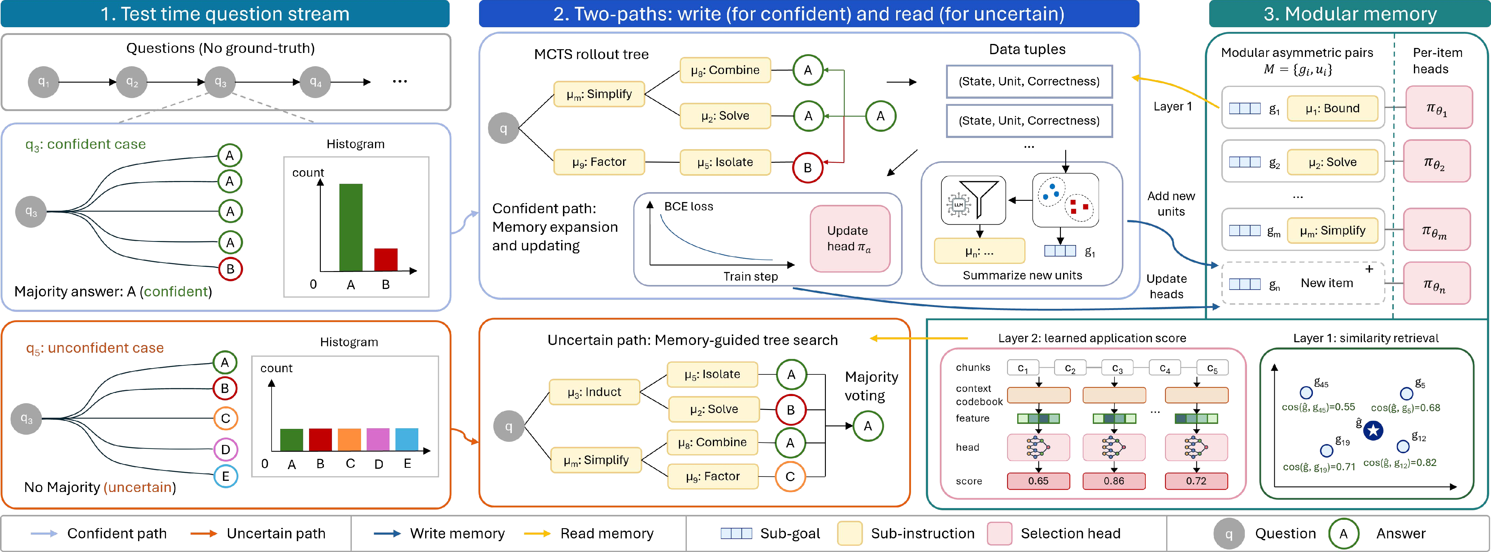
Our goal is to improve test-time reasoning by augmenting a frozen LLM with an external step-wise memory built from the model’s own reasoning experience. MILES maintains a memory \(\mathcal{M}\) of modular (sub-goal embedding, sub-instruction text) units with lightweight per-item selection heads. As the model processes a stream of test problems, MILES operates in two modes: (1) For confident samples, it incrementally expands memory and learns selection heads from rollout outcomes, enabling the system to accumulate reusable reasoning experience over time. (2) For uncertain samples, it retrieves and reranks relevant memory units through a coarse-to-fine selection mechanism to guide reasoning and improve accuracy. Figure 1 illustrates the overall framework of MILES. The remainder of this section details the four core components that realize this design.
We first define and construct modular memory units in Section [sec:mem-unit]. Building on this memory structure, Section [sec:mem-rs] introduces a coarse-to-fine selection mechanism that supports both memory expansion and training-data collection for the selection heads. Based on the collected supervision, Section [sec:learn-head] presents the learning procedure for the lightweight selection heads under limited data and incrementally expanding memory. Finally, Section [sec:test-pipe] integrates these components into a unified test-time pipeline that expands memory from confident samples and applies memory-guided tree search to uncertain samples.
3.3 Step-wise memory unit: (sub-goal, sub-instruction) pairs↩︎
A memory unit is an asymmetric pair \((g_i, u_i)\), where the sub-goal \(g_i \in \mathbb{R}^{d}\) is an embedding that summarizes the objective the sub-instruction is intended to achieve, and the sub-instruction \(u_i\) is a natural-language directive used to condition generation when the unit is applied. The memory is defined as \(\mathcal{M} = \{(g_i, u_i)\}_{i=1}^{N}\), where \(N\) grows over time as new reasoning experience is accumulated. We use \(a \in {1,\ldots,N}\) to denote the action of applying unit \((g_a, u_a)\). Each unit is associated with a learnable selection head that predicts the applicability based on previous experience.
The sub-goal serves as a retrieval key for determining whether a sub-instruction is applicable to the current reasoning state and for detecting new knowledge during test-time memory expansion (Section [sec:mem-rs]). We organize memory as a collection of modular, per-item units, enabling incremental test-time expansion: new units and their corresponding selection heads (Section [sec:learn-head]) can be added without retraining existing components, allowing memory to grow continuously with the test stream.
Memory unit summarization. Given a set of (reasoning step, step-goal) tuples collected from confident reasoning trajectories, where the step-goal describes the objective of the reasoning step and is generated by the LLM, we cluster them using k-means with the following joint distance: \[d(\mathbf{s}_{1}, \mathbf{o}_{1}; \mathbf{s}_{2}, \mathbf{o}_{2}) \;=1-\mathrm{cos}(\mathbf{s}_{1}, \mathbf{s}_{2}) \;+\; \alpha_{\text{sum}}\left[1 - \mathrm{cos}(\mathbf{o}_{1}, \mathbf{o}_{2})\right], \label{eq:dist-sum}\tag{1}\] where \(\mathbf{s}_{1,2}\) and \(\mathbf{o}_{1,2}\) denote step and step-goal embeddings, and \(\alpha_{\text{sum}}\) balances the two terms. Within each cluster, the LLM summarizes a generalized sub-instruction \(u_i\) from reasoning steps, while the average step-goal embedding defines the sub-goal \(g_i\) of the new memory unit. We also store the mean intra-cluster distance \(\overline{d}i\) to define the per-unit effective threshold \(R_{\text{effect}}^{(i)}\) (Appendix 9.1).
3.4 Coarse-to-fine memory retrieval and selection↩︎
Built upon sub-goal embeddings and selection heads, we propose a two-layer coarse-to-fine memory retrieval and selection mechanism: a lightweight similarity-based stage, followed by a learned selection head that scores each candidate using features of the full reasoning state.
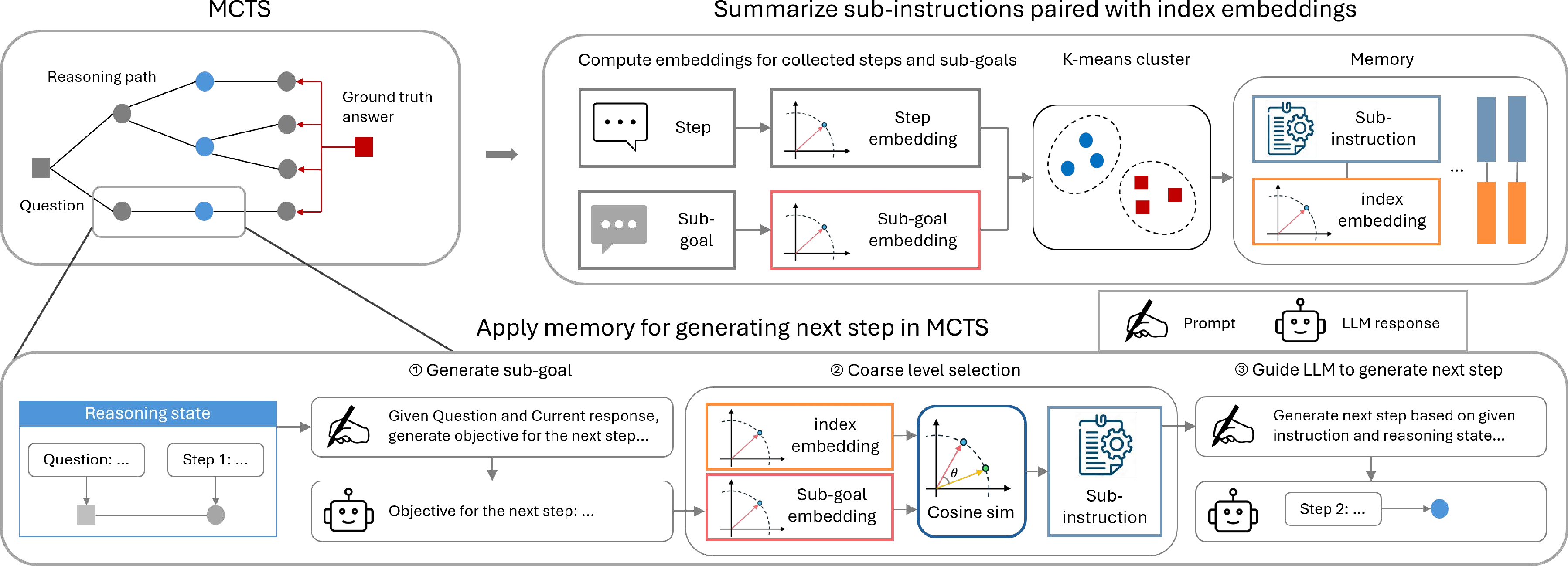
Layer 1: coarse retrieval based on sub-goal similarity. We first prompt the LLM to generate one or more candidate step-goals for the next reasoning step and compute their embeddings using a fixed embedding model. For each candidate step-goal embedding \(\hat{g}\), we compute the cosine similarity \(\mathrm{cos}(\hat{g}, g_i)\) between \(\hat{g}\) and each stored sub-goal \(g_i\) in \(\mathcal{M}\), and retrieve the most similar memory units. To avoid retrieving irrelevant units, we apply a per-unit effective threshold \(R_{\text{effect}}^{(i)} = \alpha_{\text{eff}} \cdot \overline{d}_{i}\); units with distance exceeds the threshold are excluded. If no unit matches a candidate step-goal, the LLM directly generates the next reasoning step, and the resulting (step-goal, reasoning step) pair is stored as a seed for incremental memory expansion, gradually expanding coverage over a broader range of conditions in the step-goal embedding space.
Layer 2: learned applicability scoring. Layer 1 does not incorporate selection knowledge learned from previous outcome feedback. Layer 2 addresses this limitation with a learned per-unit memory selection head \(\pi_{\boldsymbol{\theta}_{a}}(a \mid x)\) that scores the applicability of unit \(a\) in state \(x\). To identify contextual patterns most relevant to the applicability of \(a\) and to obtain a fixed-length representation of a variable-length reasoning state \(x\), we pre-compute a small set of context prototypes \(\{\mathbf{q}_{a1}, \ldots, \mathbf{q}_{an}\}\) by clustering embeddings of stored step-goals and contextual conditions from previous applications of \(a\); the full set \(\{\mathbf{q}_{ai}\}\) forms a context codebook (Appendix 10.0.0.1). Given \(x\), we split it into overlapping chunks with embeddings \(\mathbf{c}_1, \ldots, \mathbf{c}_T\) and apply the codebook via max-similarity pooling: \[\mathbf{m}_a(x) \;=\; [s_{a1}, s_{a2}, \ldots, s_{an}], \qquad s_{ai} \;=\; \max_{j \in [1, T]} \mathrm{cos}(\mathbf{q}_{ai}, \mathbf{c}_j), \label{eq:context-feature}\tag{2}\] where \(\mathbf{m}_a(x) \in \mathbb{R}^{n}\) is the context feature vector. The max-similarity construction gives a location-invariant fingerprint of the reasoning state with respect to each prototype, regardless of how long \(x\) becomes. The per-item selection head \(\pi_{\boldsymbol{\theta}_{a}}(a \mid x) = f_{\boldsymbol{\theta}_{a}}\!\bigl(\mathbf{m}_a(x)\bigr) \in [0, 1]\) is a lightweight one-vs-rest binary classifier that scores how applicable unit \(a\) is at state \(x\).
Combined score. To balance semantic relevance (Layer 1) and learned applicability (Layer 2), we combine the Layer 1 similarity score with the Layer 2 applicability score: \[\mathrm{score}(a, x) \;=\; (1 - \beta_{\text{c2f}}) \cdot \mathrm{cos}(\hat{g}, g_a) \;+\; \beta_{\text{c2f}} \cdot \pi_{\boldsymbol{\theta}_{a}}(a \mid x), \label{eq:combined-score}\tag{3}\] where \(\beta_{\text{c2f}} \in [0, 1]\) controls the relative weight of the two layers. The unit with the highest combined score is applied at the next reasoning step.
Train and apply selection heads via two-layer selection. Layer 1 selection is used on confident samples to collect sub-instruction application trajectories for training the selection heads. This enables the selection heads to learn when each sub-instruction should be applied from the LLM’s confident reasoning trajectories. For uncertain samples, Layer 1 selection first retrieves candidate memory units, after which Layer 2 selection uses the trained heads to rerank candidate sub-instructions, allowing the model to leverage knowledge learned from confident cases to guide reasoning under uncertainty.
3.5 Learning the memory selection heads↩︎
To update the selection heads for improved performance. We formulate memory selection as a sequential decision-making problem, where selecting memory unit \(a\) at reasoning state \(x\) should maximize downstream final-answer correctness. We first derive the optimal selection policy under a KL regularization constraint, then approximate it with a lightweight per-item classifier suitable for incremental test-time learning. Training data is collected from confident samples using the Layer 1 selection.
Selection objective. We formalize step-wise memory selection as a sequential decision-making problem and model the choice of which memory unit \(a\) to apply at state \(x\) as a stochastic selection policy \(\pi(a \mid x)\) over the units in \(\mathcal{M}\). Let \(p(\cdot \mid \cdot)\) denote the original LLM generation distribution and \(p_m(\cdot \mid \cdot)\) the memory-guided generation distribution. Our objective is to maximize the probability of producing a correct final answer under memory guidance: \[\max_{\pi(a \mid x)} p_m(y^*|x)=\sum\nolimits_{a} \pi(a \mid x) \cdot V(x, a), \quad V(x, a) \;=\; \mathbb{E}_{p(e \mid x, a)}\!\left[\mathbb{E}_{p_{m}(y \mid e, x)}[r]\right], \label{eq:final-obj}\tag{4}\] where \(r\) is a binary correctness indicator, \(e\) is the next reasoning step generated under the guidance of \(a\), and \(y\) is the resulting final answer. The full derivation is provided in Appendix 6.1.
Closed-form optimum under a KL constraint. Given trajectories collected by the Layer 1 data-collection distribution \(\pi_{\text{sim}}(a \mid x)\), augmenting Eq. 4 with a KL-divergence penalty \(\beta\,\mathrm{KL}\!\bigl(\pi(\cdot \mid x) \,\Vert\, \pi_{\text{sim}}(\cdot \mid x)\bigr)\) yields the following closed-form optimum [23]: \[\pi^{*}(a \mid x) \;=\; \frac{1}{Z(x)} \, \pi_{\text{sim}}(a \mid x) \cdot \exp\!\bigl(V(x, a) / \beta\bigr), \label{eq:opt-policy}\tag{5}\] where \(\beta > 0\) is the KL coefficient and \(Z(x)\) is a normalization constant ensuring that \(\pi^{*}(\cdot \mid x)\) is a valid distribution. A detailed derivation is provided in Appendix 6.2. The closed-form optimum characterizes the desired sub-instruction selection behavior but does not provide a practical mechanism for generalization beyond the sampled trajectories. We therefore train lightweight selection heads to approximate \(\pi^{*}(\cdot \mid x)\), enabling effective memory-selection patterns learned from rollout outcomes to be transferred to unseen reasoning states.
From the closed-form optimum to a tractable surrogate. Directly approximating the optimal policy in Eq. 5 is impractical because \(\pi_{\text{sim}}\) lacks a tractable density and rollout-based value estimates are noisy. We therefore approximate the policy by training one-vs-rest binary classifiers on thresholded correctness labels, encouraging the selection heads to imitate successful decisions sampled from \(\pi_{\text{sim}}(a \mid x)\). This per-item design supports incremental memory expansion without retraining existing heads. Further discussion is provided in Appendix 6.3.
Per-unit binary cross-entropy training. For each memory unit \(a\), we train its selection head \(\pi_{\boldsymbol{\theta}_{a}}(a \mid x)\) via binary cross-entropy on (state, label) pairs collected from MCTS rollouts (Section [sec:test-pipe]): \[\ell_{a}(x, \boldsymbol{\theta}_{a}; r_{a}) \;=\; -\left[\, r_{a} \cdot \log \pi_{\boldsymbol{\theta}_{a}}(a \mid x) \;+\; (1 - r_{a}) \cdot \log\!(1 - \pi_{\boldsymbol{\theta}_{a}}(a \mid x)) \,\right]. \label{eq:cond-loss}\tag{6}\] In the one-vs-rest setting, positive examples for unit \(a\) are states \(x\) at which applying \(a\) led to a correct final answer. Negative examples for unit \(a\) include: (i) states where applying \(a\) leads to an incorrect answer, and (ii) states where a different unit \(a' \neq a\) led to a correct answer. This dense step-level supervision enables effective learning under limited-data in test time. A detailed comparison with prior optimization methods is presented in Appendix 6.3.
ll cccc >cc Dataset & Model & ZS-CoT & SC & DC & BoT & Ours
& GPT-4.1-mini & 88.00 & 89.40 & 87.00 & 86.80 & 92.60
& GPT-4.1 & 87.20 & 88.00 & 83.20 & 84.80 & 91.60
& GPT-4.1-mini & 46.67 & 56.67 & 63.33 & 50.00 & 66.67
& GPT-4.1 & 40.00 & 50.00 & 53.33 & 50.00 & 53.33
& GPT-OSS-20B & 83.33 & 93.33 & 43.33 & 50.00 & 93.33
& Qwen3-30B-Instruct & 70.00 & 83.33 & 23.33 & 63.33 & 86.67
& GPT-4.1-mini & 46.67 & 53.33 & 60.00 & 40.00 & 60.00
& GPT-4.1 & 33.33 & 36.67 & 50.00 & 33.33 & 40.00
& GPT-OSS-20B & 86.67 & 90.00 & 36.67 & 33.33 & 93.33
& Qwen3-30B-Instruct & 60.00 & 70.00 & 30.00 & 53.33 & 73.33
& GPT-4.1-mini & 70.20 & 71.72 & 63.64 & 66.67 & 73.23
& GPT-4.1 & 68.94 & 68.69 & 64.65 & 61.11 & 70.71
& GPT-OSS-20B & 68.18 & 71.72 & 61.62 & 37.37 & 74.24
& Qwen3-30B-Instruct & 70.20 & 72.23 & 42.42 & 67.68 & 73.74
& GPT-4.1-mini & 82.00 & 83.50 & 83.50 & 83.00 & 85.00
& GPT-4.1 & 81.00 & 83.00 & 78.00 & 84.00 & 84.50
& GPT-OSS-20B & 85.50 & 86.50 & 79.00 & 42.00 & 87.00
& Qwen3-30B-Instruct & 87.00 & 88.50 & 63.50 & 86.00 & 88.50
& GPT-4.1-mini & 65.50 & 73.50 & 67.50 & 70.50 & 75.00
& GPT-4.1 & 75.50 & 78.50 & 72.00 & 67.50 & 80.00
& GPT-OSS-20B & 68.50 & 70.00 & 66.50 & 41.50 & 71.00
& Qwen3-30B-Instruct & 74.50 & 78.00 & 52.00 & 75.50 & 81.00
3.6 Incremental test-time memory construction and inference↩︎
In this section, we integrate the previous components into a unified pipeline, including: (1) incrementally constructing memory and learning sub-instruction selection from confident samples, and (2) applying memory-guided reasoning to uncertain samples.
Confidence-based routing of test samples. In the test-time setting, samples arrive sequentially without ground-truth labels. For each test sample \(q\), we generate \(K\) independent LLM responses and check whether they agree on a final answer. Samples whose responses converge to a consistent answer are treated as confident samples: the majority-vote answer serves as a pseudo-label for evaluating MCTS rollouts, and the resulting trajectories are used to expand memory and train the selection heads. Samples with inconsistent responses are instead routed to memory-guided tree search using the learned heads. Intuitively, confident samples provide a reliable supervisory signal, whereas the LLM should leverage prior experience to guide reasoning when it is uncertain about a sample.
Data collection and memory expansion via MCTS on confident samples. For each confident sample we run MCTS over the reasoning tree to collect training data for the selection heads. At each tree node (a reasoning state \(x\)), we use the Layer 1 sub-goal similarity to sample candidate memory units to apply, run the LLM to expand the chosen step, and propagate correctness signals from rollouts evaluated against the pseudo-label. The detailed MCTS procedure is presented in Appendix 8.1.
The collected (step-goal, reasoning step) pairs (Section [sec:mem-rs]) are summarized into new memory units as described in Section [sec:mem-unit]. Data collection uses only Layer 1 similarity-based sampling via \(\pi_{\text{sim}}\) to avoid bias toward the current selection heads and preserve trajectory diversity. The resulting tuples are stored in per-unit datasets \(\mathcal{D}_{a} = {(x_{j}, r_{a,j})}\) for training the corresponding selection heads \(\pi_{\boldsymbol{\theta}_{a}}\) with the BCE loss in Eq. 6 . The detailed training procedure is described in Appendix 10.
Memory-guided tree search for uncertain samples. For samples whose initial \(K\) responses are inconsistent, we apply a multi-stage memory-guided tree search similar to [19]. At each stage, a sub-context is sampled from existing reasoning chains, candidate step-goals are generated, and memory units are retrieved and ranked using the combined score in Eq. 3 . The top-ranked unit is then applied to expand the reasoning trajectory, and the resulting branch is added to the response pool. As search progresses, longer sub-contexts are used to guide later reasoning steps. The final answer is determined by majority voting over all generated responses. Details of the memory-guided tree search procedure are provided in Appendix 8.2.
4 Experiments↩︎
4.1 Main results on LLM reasoning: accuracy, efficiency, and transferability↩︎
Datasets, models and evaluation. We evaluate on six reasoning benchmarks spanning competition mathematics and graduate-level academic exams: MATH-500 [24], AIME 2024, AIME 2025, GPQA-Diamond [25], and the Physics and Engineering
subsets of MMLU-Pro [26]. Following [9], we randomly sample 200 instances from each MMLU-Pro subset and evaluate the remaining datasets in full. We evaluate MILES on four backbone LLMs spanning proprietary and open-weight families: GPT-4.1, GPT-4.1-mini [27], Qwen3-30B-Instruct [28], and
GPT-OSS-20B [29]. For fair comparison, the same backbone is used for both reasoning and memory construction across all methods within each row.
All embeddings in MILES are computed using the embedding model text-embedding-3-small. Final-answer accuracy is used as the evaluation metric.
Baselines. We compare MILES against test-time memory methods, including Buffer-of-Thoughts (BoT) [5] and Dynamic CheatSheet (DC) [9], as well as two standard baselines: zero-shot Chain-of-Thought (ZS-CoT) [30] and Self-Consistency (SC) [2]. Additional comparisons with memoryless test-time scaling methods are provided in Appendix 11.

MILES configuration. Across all experiments, MILES uses the same component design described in Section [sec:method], with per-item selection heads implemented as an ensemble of 10 independently trained 3-layer MLPs for robust inference. Additional implementation details are provided in Appendix 14. Since majority-voting results are stable, we omit error bars.
Table ¿tbl:tab:test-time? shows that MILES matches or outperforms baseline works across all six benchmarks and four backbones, with consistent gains on both math (MATH-500, AIME 2024–2025) and academic (GPQA-Diamond, MMLU-Pro Physics/Engineering) datasets. The improvements are especially pronounced on smaller open-weight backbones (GPT-OSS-20B and Qwen3-30B-Instruct), where the sample-level memory baselines BoT [5] and DC [9] fail to outperform zero-shot CoT due to overly complex prompt. In near-saturated settings (e.g., GPT-OSS-20B on AIME 2024 at 93.33%), MILES matches self-consistency without degradation, demonstrating its effectiveness and robustness. We note that the strong performance of DC on the AIME datasets mainly comes from its use of coding; additional details are provided in Appendix 11.
R0.5
ll >cc Dataset & Auxiliary model & Accuracy
& no-auxiliary model & 60.00
& Qwen3-30B-Instruct & 66.67
& Qwen3-4B-Instruct & 63.33
& GPT-4.1-mini & 66.67
& no-auxiliary model & 50.00
& Qwen3-30B-Instruct & 60.00
& Qwen3-4B-Instruct & 56.67
& GPT-4.1-mini & 60.00
Performance under different computation budget. We probe how accuracy scales with test-time compute by plotting accuracy against response-token cost on AIME 2024 and AIME 2025 with GPT-4.1-mini, comparing MILES to representative memoryless test-time scaling methods: Self-Consistency [2], Tree-of-Thoughts [3], rStar [4], and DORA [20]. As shown in Figure 2, MILES benefits more from increased computation budgets by constructing additional memory units (Section [sec:rollouts]), dominating the accuracy/token frontier and continuing to improve as the budget grows, whereas the baselines quickly plateau. This highlights the effectiveness of reusing cross-problem memory, which captures knowledge that per-problem scaling alone cannot.
Cross-model transfer. Because MILES operates on textual memory representations, memory construction need not use the same model as the reasoning backbone. We evaluate cross-model transfer on AIME 2024 and AIME 2025 using GPT-4.1-mini as the reasoning backbone: the backbone generates the first 10 self-consistency rollouts for routing, while an auxiliary model generates the next 40 rollouts for memory construction. Table ¿tbl:tab:tranfer? shows that auxiliary trajectories from Qwen3-30B-Instruct, Qwen3-4B-Instruct, and GPT-4.1-mini itself all improve over the no-auxiliary baseline, demonstrating that memory constructed by open-weight auxiliary models transfers effectively to a stronger frozen backbone.
R0.5
ll >cc Dataset & Auxiliary model & Accuracy
& no memory & 23.08
& Qwen3-30B-Instruct & 30.77
& GPT-4.1-mini & 38.46
& no memory & 48.39
& Qwen3-30B-Instruct & 58.06
& GPT-4.1-mini & 54.84
Offline memory construction with training set. When a separate labeled set is available, memory can be built ahead of time and memory-guided tree search applied only to the most uncertain test samples (Section [sec:test-pipe]). We evaluate our method on AIME 2025 using memory constructed from AIME 2020–2024, and on GPQA-Diamond [25] using memory constructed from the non-Diamond GPQA split, reporting accuracy on the 13 and 31 most uncertain test samples, respectively. Table ¿tbl:tab:train-tranfer? shows that memory pre-built by either Qwen3-30B-Instruct or GPT-4.1-mini itself substantially improves over the no-memory baseline. These results demonstrate that MILES learns reusable problem-solving knowledge that transfers across different models and samples within the same domain.
4.2 Ablation study↩︎
R0.6
lccc >cc Dataset & Exp. ID & Layer 1 & Layer 2 & Accuracy
& 1 & & & 60.00
& 2 & & & 63.33
& 3 & & & 63.33
& 4 & & & 66.67
& 5 & & State sim. & 63.33
& 6 & & LLM rerank & 60.00
& 1 & & & 53.33
& 2 & & & 53.33
& 3 & & & 56.67
& 4 & & & 60.00
& 5 & & State sim & 56.67
& 6 & & LLM rerank & 53.33
Effectiveness of each component in two-layer selection. To evaluate the two-layer selection mechanism, we conduct experiments on AIME 2024 and AIME 2025 with GPT-4.1-mini. When both layers are disabled, no memory is constructed and no selection heads are trained. We further compare Layer 2 against two alternative rerankers: (i) state-similarity reranking, which scores candidates by the similarity between the current reasoning-state embedding and the average embeddings of previously successful states; and (ii) LLM-prompt reranking, which prompts LLM with the current reasoning state and the Layer-1 candidate sub-instructions and asks it to identify the most applicable candidate.
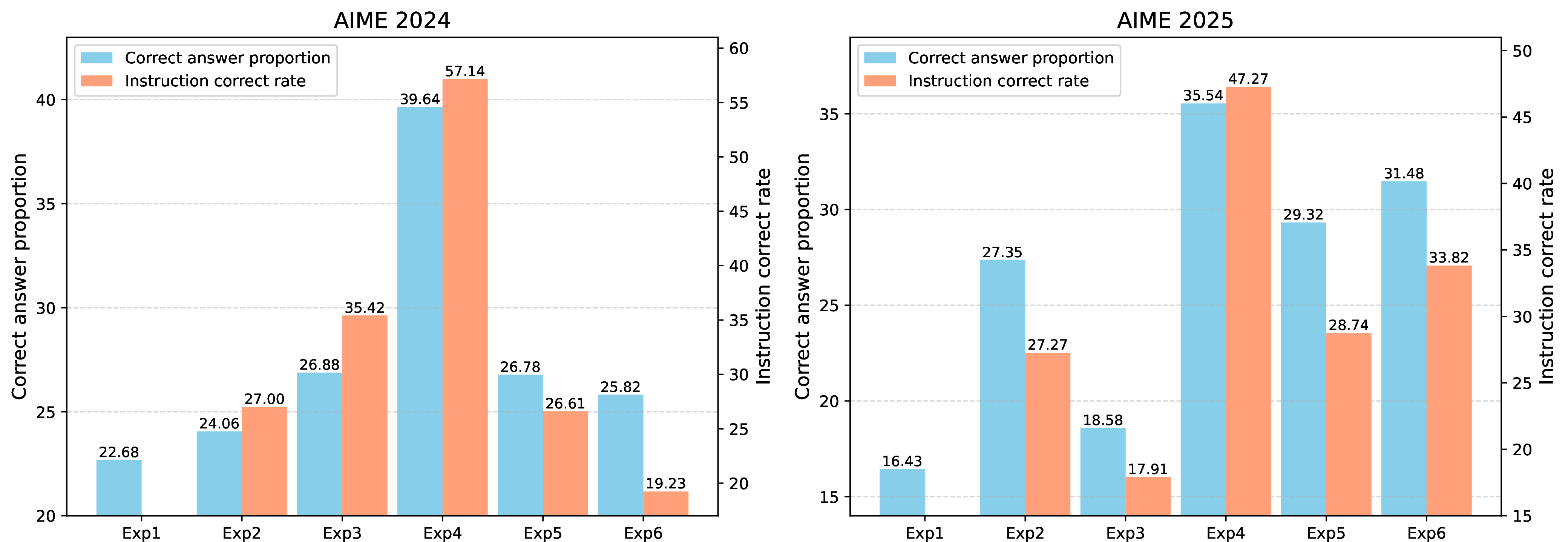
Table ¿tbl:tab:ablation? shows that combining both layers (Exp 4) yields the best accuracy on both datasets, while disabling either layer (Exp 2–3) reduces performance. Disabling both layers causes accuracy to fall close to the self-consistency baseline, especially on AIME 2025. Among alternative rerankers, state-similarity reranking (Exp 5) recovers a large fraction of the learned classifier’s gain, while LLM-prompt reranking (Exp 6) fails to improve over the no-reranker baseline, indicating that the learned classifier captures signal beyond what either prompting or surface-state similarity provides. These results highlights the effectiveness of our two-layer selection mechanism.
We further inspect reasoning trajectories using two metrics: correct-answer proportion (fraction of trajectories that produce the correct final answer) and sub-instruction accuracy (fraction of sub-instruction applications that lead to a correct final answer), on samples near the correct/incorrect decision boundary where small effects matter most. Figure 3 shows that our full method (Exp 4) performs best on both metrics. The gaps between Exp 4 and Exp 1–3 validate the asymmetric memory and two-layer selection design, as well as between Exp 4 and Exp 5–6 validate the learned heads over alternative rerankers.
| Dataset | Rollouts | Mem. size | Accuracy |
|---|---|---|---|
| AIME 2024 | 20 | 9 | 60.00 |
| 30 | 15 | 66.67 | |
| 40 | 20 | 66.67 | |
| AIME 2025 | 20 | 10 | 53.33 |
| 30 | 19 | 56.67 | |
| 40 | 25 | 60.00 |
R0.5
Effect of MCTS rollouts. MILES summarizes sub-instructions in memory and collects classifier-training data via MCTS on confident samples; we therefore study how the rollout budget affects both the resulting memory size and the final accuracy. We sweep rollouts \(\in \{20, 30, 40\}\) on AIME 2024 and AIME 2025 with GPT-4.1-mini and report results in Table 1.
More rollouts yield both a larger memory with more sub-instruction units and higher accuracy. A larger number of sub-instructions corresponds to better coverage of the step-goal embedding space (Section [sec:mem-rs]). These results suggest that improved coverage leads to higher performance, and further demonstrate the effectiveness of our memory selection strategy.
| Dataset | Sample order | Accuracy | |
|---|---|---|---|
| 3-4 | 20 rollouts | 40 rollouts | |
| AIME 2024 | default | 60.00 | 66.67 |
| simple-to-hard | 66.67 | 66.67 | |
| hard-to-simple | 63.33 | 66.67 | |
| AIME 2025 | default | 53.33 | 60.00 |
| simple-to-hard | 60.00 | 60.00 | |
| hard-to-simple | 56.67 | 63.33 | |
R0.6 4pt
Impact of sample order. Because MILES updates memory online from confident samples (Section [sec:test-pipe]), sample order affects how knowledge is accumulated and reused. To evaluate the robustness of the MILES under different sample orders, we conduct experiments on AIME 2024 and AIME 2025 with GPT-4.1-mini under three sample orders: the default question-index order, easiest-to-hardest, and hardest-to-easiest, using two MCTS rollout budgets (20 and 40 per confident sample). Sample difficulty is defined by the proportion of correct answers across self-consistency rollouts. Results are in Table 2.
Under the limited rollout budget (20 per sample), the easy-to-hard order achieves the highest accuracy on both datasets, suggesting that solving easier samples first allows MILES to accumulate useful memory before encountering harder ones. With 40 rollouts, the performance gap largely disappears, indicating that the method becomes effectively order-insensitive once sufficient confident-sample data has been collected.
Additional design ablations and analyses are provided in Appendix 11.
5 Conclusion↩︎
In this work, we propose MILES, a framework for test-time self-improvement that incrementally accumulates and composes reusable step-wise reasoning experience. By learning memory-selection patterns from confident trajectories and transferring them to uncertain reasoning states, MILES enables correctness-optimized memory composition without parameter updates, external supervision, or fixed action spaces. Extensive experiments across multiple reasoning benchmarks demonstrate its effectiveness, robustness, and transferability. These results suggest that learning reusable memory-selection knowledge is a promising direction for building continually improving reasoning systems.
Limitations and future work. MILES relies on the instruction-following capability of the underlying LLM and requires rollout-based data collection, which introduces additional computational overhead. This cost can be reduced by using auxiliary models for trajectory generation (Section [sec:transfer]). Future work includes combining MILES with self-refinement methods [6], [11] to improve instruction quality and with hierarchical memory [21], [31] to improve selection efficiency.
6 Objective formulation and optimization↩︎
6.1 Memory retrieval objective↩︎
Inspired by the formulations of prior works [32], [33], we formalize sub-instruction selection as a sequential decision-making problem, where the objective is to maximize the probability of generating the correct solution by optimizing the instruction selection function. At each step, we model the effect of selecting a sub-instruction \(a\) on generating the next reasoning step \(e\) as \[p_m(e|x)=\sum_a p(e|x,a)\pi(a|x)=\mathbb{E}_{\pi(a|x)}\left[p(e|x,a)\right], \label{eq:step-gen-apd}\tag{7}\] where \(\pi(a|x)\) denotes the instruction selection function conditioned on the reasoning state \(x\), \(p(\cdot|\cdot)\) is the generation probability of LLM, and \(p_m(\cdot|\cdot)\) denotes the generation probability conditioned on sub-instructions. The reasoning state \(x\) consists of the question \(q\) and the reasoning trajectory generated so far.
Under the causal decoding mechanism, subsequent reasoning steps are conditioned on the current reasoning state and the newly generated step. Thus, the probability of generating the final solution \(y\) can be written as \(p_m(y|x,e)\). By the chain rule of probability, \[p_m(y,e|x)=p_m(y|e,x)\cdot p_m(e|x), \label{eq:prob-chain}\tag{8}\] which allows us to express the probability of generating the final solution as \[\begin{align} p_m(y|x)=&\int p_m(y,e|x)de \\ =&\int p_m(y|e,x)\cdot p_m(e|x)de \\ =&\int p_m(y|e,x)\left(\sum_a p(e|x,a)\pi(a|x)\right)de \\ =&\sum_a \left(\pi(a|x)\int p_m(y|e,x)\cdot p(e|x,a)de\right) \\ =&\sum_a \pi(a|x)\cdot \mathbb{E}_{p(e|x,a)}[p_m(y|e,x)]. \end{align} \label{eq:gen-obj-apd}\tag{9}\] Our objective is to maximize the probability of generating the correct final solution \(y^*\) by optimizing \(\pi(a|x)\), while keeping the LLM parameters fixed. Therefore, our optimization objective is \[\max_{\pi(a|x)}\;p_m(y^*|x)=\sum_a \pi(a|x)\cdot \mathbb{E}_{p(e|x,a)}[p_m(y^*|e,x)]. \label{cjmdgozr}\tag{10}\]
The effect of selecting an instruction at the current step propagates through subsequent reasoning steps and influences the final answer. However, \(p_m(y^*|e,x)\) is intractable in practice. Instead of explicitly modeling future memory selections, we approximate their impact using the expected correctness of the final answer, following the standard reinforcement learning practice of using rollout returns to evaluate intermediate decisions. Therefore, we propose to approximate \(p_m(y^*|e,x)\) using a binary correctness indicator \(r\in \{0,1\}\), defined as \[r=\begin{cases} 1, & y=y^*,\\ 0, & y\neq y^*. \end{cases}\] Because \(r\) follows a Bernoulli distribution with success probability \(p_m(y^*|e,x)\). we approximate \(p_m(y^*|e,x)\) by the expectation over \(r\), \[p_m(y^*|e,x)=\mathbb{E}_{p_m(y|e,x)}[r].\] This approximation reduces the sequential decision problem to evaluating the expected return of a one-step decision, while implicitly accounting for future reasoning through rollout-based reward signals. Substituting this into the objective in Eq. 9 yields \[\max_{\pi(a|x)} p_m(y^*|x)=\sum_a \pi(a|x)\cdot V(x,a),\quad V(x,a)=\mathbb{E}_{p(e|x,a)}\left[\mathbb{E}_{p_m(y|e,x)}[r]\right]. \label{eq:final-obj-apd}\tag{11}\] where \(V(x,a)\) represents the expected correctness of the final answer when selecting instruction \(a\) under reasoning state \(x\).
6.2 Optimal teacher policy↩︎
During data collection, we select sub-instructions based on the similarity between step-goal embeddings and sub-goal. Let this sampling policy be denoted as \(\pi_{\text{sim}}\). Following [23], we optimize a target policy \(\pi(a|x)\) under a KL-regularized objective: \[\begin{align} \arg \max_{\pi(a|x)}& \;\int d_{\pi_{\text{sim}}}(x)\left(\sum_a \pi(a|x)\cdot V(x,a)\right)dx \\ \mathrm{s.t.}& \;\mathrm{D_{\text{KL}}}(\pi(a|x)||\pi_{\text{sim}}(a|x))\le \epsilon,\quad \forall \;x \\ &\;\sum_a \pi(a|x)=1,\quad \forall \;x. \end{align} \label{eq:opt-obj-apd}\tag{12}\] where \(d_{\pi_{\text{sim}}}(x)\) denotes the state distribution induced by \(\pi_{\text{sim}}\), and \(\pi(a|x)\) is the policy to be optimized.
Following the derivation in [23], we form the corresponding Lagrangian: \[\begin{align} \mathcal{L}(\pi,\beta_{\text{KL}},\alpha_{\text{prob}})=&\int d_{\pi_{\text{sim}}}(x)\left(\sum_a \pi(a|x)\cdot V(x,a)\right)dx \\ &+\beta_{\text{KL}}\left(\epsilon-\int d_{\pi_{\text{sim}}}(x)\cdot \mathrm{D_{\text{KL}}}(\pi(a|x)||\pi_{\text{sim}}(a|x))dx\right) \\ &+\int \alpha_{x}\left(1-\sum_a\pi(a|x)\right)dx, \end{align}\label{eq:lagrangian}\tag{13}\] where \(\beta_{\text{KL}}\) and \(\alpha_{\text{prob}}=\{\alpha_{x}|\forall x\}\) are Lagrange multipliers for the KL and normalization constraints, respectively. Setting \(\partial \mathcal{L} / \partial \pi(a|x) = 0\) yields the optimal policy: \[\pi^*(a|x)=\frac{1}{Z(x)}\pi_{\text{sim}}(a|x)\exp\left(V'(x,a)\right),\quad V'(x,a)=\frac{1}{\beta_{\text{KL}}}V(x,a),\label{eq:opt-policy-apd}\tag{14}\] where \(Z(x)\) is the normalization constant: \[Z(x)=\exp\left(\frac{\alpha_{x}}{d_{\pi_{\text{sim}}}(x)\beta_{\text{KL}}}+1\right) =\sum_a \left(\pi_{\text{sim}}(a|x)\exp\left(\frac{1}{\beta_{\text{KL}}}V(x,a)\right)\right),\] ensuring that \(\pi^*(a|x)\) is a valid probability distribution. Notably, DPO [34] derives a similar form of the optimal policy via a different formulation. The optimal form \(\pi^{*}(a \mid x)\) is invariant to subtracting a state-dependent baseline from \(V(x, a)\) in the exponent, since any such baseline is absorbed into \(Z(x)\); we therefore use the bare value \(V(x, a)\) rather than an advantage.
6.3 Practical optimization objective↩︎
Training objective. Our goal is to train the selection heads to approximate the optimal policy in Eq. 14 . However, direct optimization using the weighted maximum-likelihood approach of [23] is impractical because the sampling policy \(\pi_{\text{sim}}(a|x)\) is intractable and rollout-based value estimates become noisy when amplified by small \(\beta_{\text{KL}}\). We therefore approximate the optimal policy using binary correctness labels, where \(r_a=1\) if selecting instruction \(a\) leads to the correct final answer, and \(r_a=0\) otherwise.
In Eq. 14 , the optimal policy \(\pi^*(a|x)\) reweights the sampling policy \(\pi_{\text{sim}}(a|x)\) according to the value \(V(x,a)\). Approximating \(\pi^*(a|x)\) therefore encourages the selection heads to assign higher probabilities to instruction \(a\) selected by \(\pi_{\text{sim}}(a|x)\) that lead to high-value outcomes and lower probabilities to those that lead to poor outcomes. Our binary surrogate follows the same intuition by training the selection heads to distinguish successful trajectories sampled from \(\pi_{\text{sim}}(a|x)\) from unsuccessful ones.
Per-item selection head training. To support incrementally expanding memory, we train a separate selection head for each sub-instruction rather than a single joint classifier. This design allows newly added instructions to be trained independently without retraining existing classifiers. Specifically, we decompose selection into one-vs-rest binary classification problems. For instruction \(a\), positive samples are states where applying \(a\) leads to a correct final answer, while negative samples include states where applying \(a\) leads to an incorrect answer or where another instruction succeeds instead. We train each classifier using binary cross-entropy: \[\ell(x,\boldsymbol{\theta};r_a)=-\left[r_a\cdot \log\left(\pi_{\boldsymbol{\theta}}(a|x))\right)+(1-r_a)\cdot \log\left(1-\pi_{\boldsymbol{\theta}}(a|x))\right)\right], \label{eq:bce-loss}\tag{15}\] where \(r_a\in{0,1}\) denotes the binary label for instruction \(a\). This objective encourages high scores for instructions that lead to correct solutions while suppressing unsuitable ones.
Collecting diverse training data. In our data collection procedure, we select sub-instructions based on the similarity between step-goal embeddings and sub-goal, without relying on predictions from the selection heads. This design aims to mitigate selection bias and promote data diversity. In contrast, using the selection head during data collection would bias the sampled applications toward its current preferences, resulting in less informative and less diverse training data. By decoupling data collection from the selection head, we obtain a more diverse set of application trajectories, which enables the selection head to more effectively learn when to apply each sub-instruction.
Connection to and departure from prior derivations. The closed-form Eq. 14 we use is the same form as the optimum derived in [23] for advantage-weighted regression and, in a different domain, in [34] for direct preference optimization. We share with these works only the derivation of the optimum.
In AWR [23], the policy is iteratively improved by applying the current policy and updating it toward a new optimal policy. However, in our setting, iteratively refining the policy for a single question may introduce bias and degrade performance on other questions, while updating the policy across all existing querie questions is computationally expensive. In practice, we replace AWR’s soft advantage-weighted maximum-likelihood surrogate with a binary cross-entropy surrogate over per-item classifiers, and we do not perform iterative policy improvement: training data is collected once via MCTS rollouts on confident samples (Section [sec:test-pipe]), and the per-item heads are trained offline. We therefore avoid iterative policy updates.
EXIT [35] also employs iterative updates: in each iteration, it collects trajectories via MCTS and trains the policy to imitate these trajectories, biasing future exploration toward more promising decisions. In contrast, we estimate the optimal policy using the AWR formulation and train selection heads to directly imitate this policy, eliminating the need for repeated MCTS-based iterations.
7 Broader context and related work↩︎
7.1 Step-wise guidance for LLM reasoning↩︎
Different reasoning strategies should be applied as the reasoning state evolves. ArcMemo [14] selects modular concepts by prompting the reasoning model, while CoM [36] prompts a meta-agent LLM to select a predefined cognitive mode for the next reasoning step as the reasoning process progresses.
Process reward models (PRMs) provide reliable evaluations of reasoning trajectories [37]. PGTS [38] trains a graph neural network to select tree-search actions with the goal of maximizing cumulative rewards computed by a PRM or LLM-based evaluation. RLoT [39] formulates the reasoning process as a Markov Decision Process (MDP) and trains an RL agent to predict the next logic block based on the current reasoning state, using a PRM as a teacher to guide the training of the RL agent.
In contrast to these approaches, our method enables adaptive step-wise memory selection without requiring an additional PRM to guide training or inference. Moreover, our approach progressively accumulates knowledge as experience grows, rather than restricting the LLM to a fixed set of predefined logic blocks.
7.2 Self improvement for LLM reasoning↩︎
Self-improvement methods aim to enhance LLM reasoning performance using the model’s own generations. STaR [7] prompts the LLM to generate reasoning chains and then fine-tunes the model on trajectories that lead to correct answers. B-STAR [8] further improves performance by adaptively balancing exploration and exploitation. While effective, these approaches require updating model parameters, which is infeasible for closed-source models.
SELF-REFINE [40] and Reflexion [11] instead iteratively refine LLM responses using self-generated feedback. These methods improve performance by modifying the context rather than updating model parameters. However, their effectiveness largely depends on the quality of the generated feedback. BRIDGE [41] iteratively generates and selects influential demonstrations to enhance the reasoning capability of in-context learning.
Compared to existing approaches, our method constructs and learns to select reusable step-wise memory from confident samples, and then applies this memory to guide reasoning on uncertain samples. Unlike prior self-improvement methods, our approach requires neither model parameter updates nor additional supervision signals or self-feedback. As a result, it is applicable to both open-source and closed-source models in the test-time setting. Moreover, because our method relies on reusable memory derived from previous experience rather than iterative self-feedback, its effectiveness is less dependent on the quality of generated feedback.
7.3 Retrieval-augmented generation for reasoning↩︎
Retrieval-augmented generation (RAG) methods dynamically retrieve external information relevant to an input query and condition generation on the retrieved content. ReAct [42] combines internal and external knowledge by prompting the LLM to search and retrieve information from Wikipedia, aiming to improve reasoning through external knowledge access. HARR [43] formulates multi-hop retrieval as a Markov Decision Process and optimizes the retrieval policy to maximize the F1 score of LLM responses using GRPO [44]. However, existing retrieval-based methods typically operate on a fixed corpus and rely on large-scale training data. In contrast, our work focuses on dynamically expanding memory, where each step-wise instruction is associated with only limited training data.
Rather than retrieving from a fixed corpus, our method incrementally accumulates reusable knowledge by constructing and learning to select step-wise memory. Furthermore, our training framework employs dense step-wise supervision with a one-vs-rest objective, enabling effective learning from limited data while supporting incremental memory expansion during test time.
7.4 Test-time scaling for LLM reasoning↩︎
Test-time scaling methods improve model performance by allocating additional computation during inference without modifying model parameters. Chain-of-Thought (CoT) prompting [1] improves the reasoning ability of large language models (LLMs) by prepending manually crafted reasoning examples to the target question. [45] shows that longer reasoning chains consistently improve reasoning performance. Agarwal et al. [46] further demonstrate that increasing the number of few-shot demonstrations mitigates pretraining bias and enhances reasoning ability.
Generating and aggregating multiple responses during inference can further improve reasoning performance. Self-Consistency (SC) [2] aggregates multiple reasoning trajectories to produce more reliable answers.
Structured-search methods for reasoning explore multiple step-level continuations and select among them using value or process rewards. Tree-of-Thought (ToT) [3] and Graph-of-Thought (GoT) [18] introduce structured exploration strategies that improve reasoning performance while reducing computational cost. rStar [4] explores reasoning states using human-like actions within an MCTS framework and selects trajectories based on mutual consistency. Tree-BoN [19] reduces the computational cost of tree search by expanding only promising reasoning chains. DORA [20] adaptively allocates rollout budgets based on PRM scores and trajectory similarity, assigning more computation to reasoning states with lower similarity and higher PRM scores.
However, these methods search over memoryless LLM rollouts without reusable cross-problem knowledge guiding expansion. In contrast, MILES integrates learned, reusable step-level memory into the search, where selection heads choose which sub-instruction to apply at each expansion step.
8 Detailed method pipeline↩︎
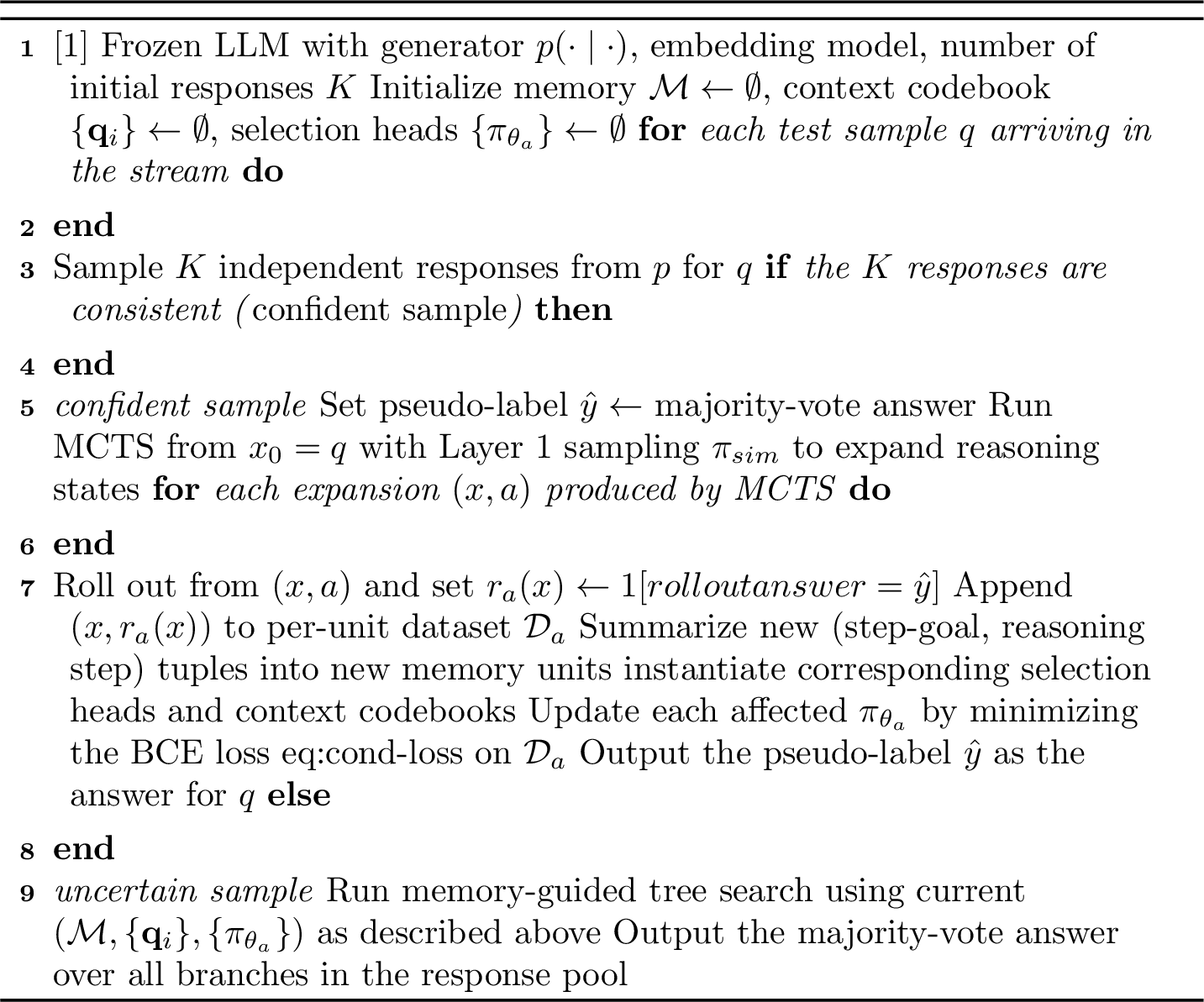
Algorithm. Algorithm 4 summarizes one pass through the test stream.
8.1 Detailed MCTS pipeline↩︎
As discussed in [47], [48]. MCTS enables step-wise evaluation while balancing exploration and exploitation. Following [49]–[51], our MCTS procedure consists of four main phases: selection, expansion, simulation, and backpropagation. Each node represents a reasoning state corresponding to a partial response, with the root node representing the question \(q\). Each edge denotes the transition between two reasoning states.
Selection. Starting from the root node, the MCTS algorithm recursively selects nodes for expansion until reaching a leaf node using the Upper Confidence Bound for Trees (UCT) criterion [52]: \[\mathrm{UCT}(v)=\frac{Q(v)}{N(v)}+C\cdot \sqrt{\frac{\ln N(\mathrm{parent}(v))}{N(v)}}, \label{eq:uct}\tag{16}\] which balances exploration and exploitation when selecting nodes for expansion. Here, \(Q(v)\) denotes the accumulated reward of node \(v\), \(N(v)\) and \(N(\mathrm{parent}(v))\) denote the visit counts of node \(v\) and its parent node, respectively, and \(C\) is a scalar hyperparameter controlling the exploration–exploitation trade-off. Larger values of \(C\) encourage selecting nodes with fewer visits, promoting exploration, while smaller values favor nodes with higher rewards, promoting exploitation. In our setting, the reward is defined as the binary correctness of the final answer, and rewards are backpropagated through all nodes along the reasoning path.
Expansion. Previous work typically expands a selected node by applying an action from a predefined action space. In contrast, our method generates the next reasoning step by applying a sub-instruction rather than relying on a fixed action space. These instructions are selected based on the similarity between step-goal embeddings and sub-goals. The expansion phase therefore collects application data for sub-instructions, which is subsequently used to train the selection heads.
Simulation. During the simulation phase, the LLM is prompted to complete the reasoning process and produce a final answer, which is then used to evaluate correctness. In our formulation, each node corresponds to a reasoning state. For a reasoning chain with \(n\) steps, there are up to \(n\) nodes along the reasoning path, where the \(i\)-th node contains the first \(i\) reasoning steps. To prevent excessive rollouts at large depths and maintain diversity in the contexts where sub-instructions are applied, we divide the simulated reasoning path into equal segments and merge multiple steps into a single node, keeping the total search depth fixed.
Backpropagation. After each simulation, the generated answer is evaluated and the leaf node is assigned a binary correctness signal. This signal is then propagated back through all nodes along the reasoning path leading to the final answer, refining the estimated quality of each node and guiding node selection in subsequent search iterations.
During the initial rollouts from the root node, we do not apply sub-instructions. This stage is therefore equivalent to self-consistency [2], and is used to estimate a pseudo ground-truth answer via majority voting. Subsequent backpropagation is then performed based on this estimated answer. Overall, MCTS enables efficient exploration of reasoning trajectories while collecting sub-instruction application data for training the selection heads. The sub-instruction trajectories explored during MCTS are collected as training data for the selection heads. The detailed MCTS procedure is described in Alg. 6.

8.2 Detailed memory-guided tree search pipeline↩︎
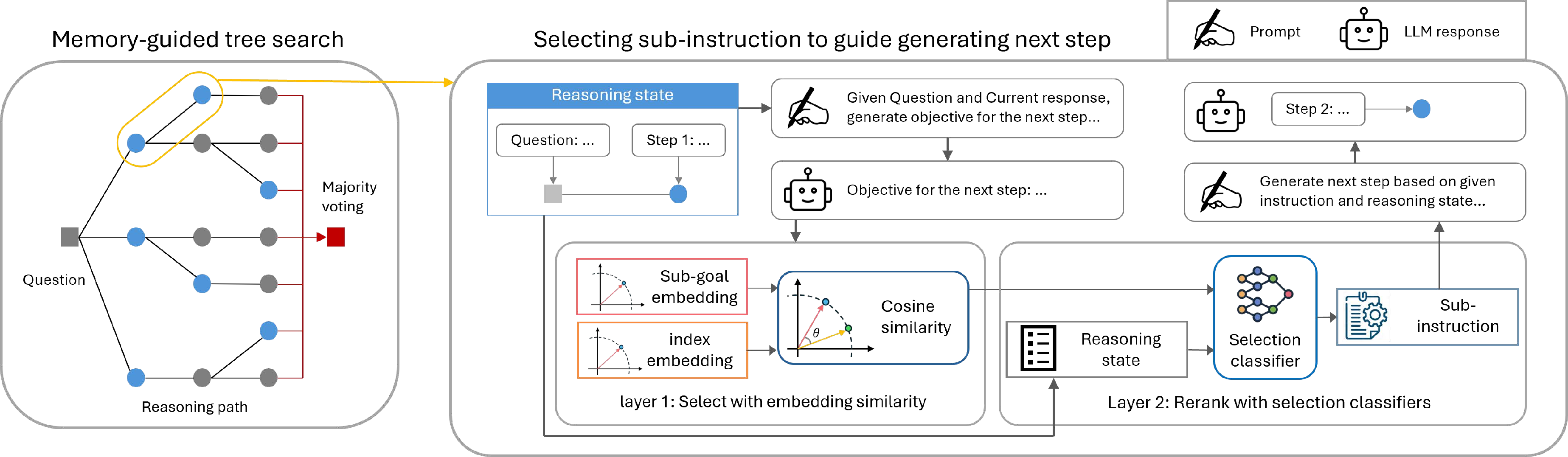
When the estimated answers are not consistent on given question, the estimated ground-truth answer and may not be correct and the correctness feedback may be noisy. As discussed in Section 8.1, the reward backpropagation and selection in MCTS may bias the expansion towards incorrect answer. Therefore, we do not apply MCTS when model is uncertain.
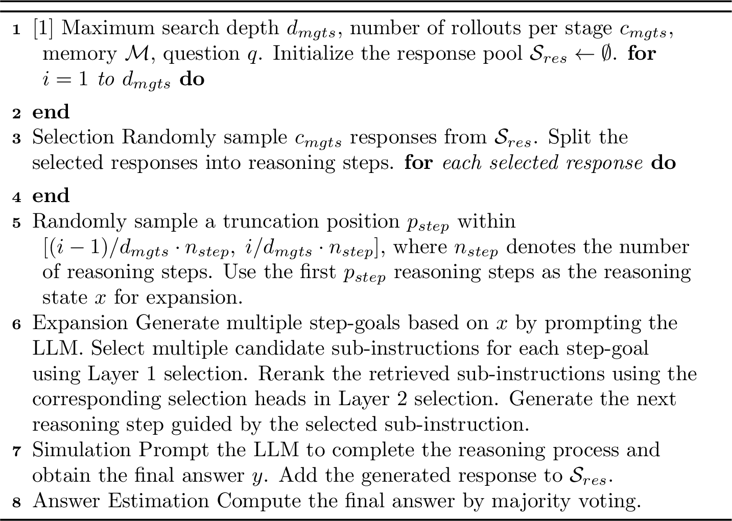
During memory-guided tree search, we apply a two-layer selection mechanism to choose sub-instructions for generating the next reasoning step given the current reasoning state. Starting from the question, we iteratively expand reasoning chains over multiple stages while maintaining a response pool that stores all generated trajectories.
At each stage, we randomly sample a sub-context from the response pool and combine it with the question to form the reasoning state. Based on this state, we select sub-instructions and guide the LLM to generate the next reasoning step. The LLM then completes the reasoning, and the resulting trajectory is added back to the response pool. As more sub-instructions are applied, we progressively increase the length of the sub-context, allowing the reasoning state to incorporate previously guided steps. Similar to MCTS, each node corresponds to a reasoning state and each edge represents a transition between states, with the question serving as the root node.
Our method predicts the applicability of sub-instructions based on the current reasoning state, but does not evaluate the overall quality of the reasoning state, unlike PRM-based methods [19], [20], [49]. As a result, we randomly select expansion positions during search. In contrast to TreeBoN [19], we do not prune branches, since the quality of a reasoning trajectory cannot be reliably determined. The detailed memory-guided tree search procedure is described in Alg. 8.
9 Memory construction details↩︎
9.1 Effective threshold↩︎
The effective threshold is designed to regulate the application of sub-instructions based on the similarity between step-goal embeddings and sub-goals. We assume that higher similarity between an step-goal embedding and the sub-goal indicates that the corresponding sub-instruction is more suitable to apply.
Each sub-instruction may have a different effective threshold. Intuitively, if a sub-instruction is summarized from a more dispersed cluster of (step-goal, reasoning step) pairs, it is more general and can be applied under a wider range of conditions. In contrast, instructions derived from tightly clustered pairs are more specialized and should be applied more selectively. Based on this intuition, we compute the effective threshold according to the distribution of the corresponding cluster.
Specifically, for each sub-instruction summarized from a cluster of (step-goal, reasoning step) pairs, we first compute the normalized distance between the sub-goal and other step-goal embeddings in the cluster as \[d(\mathbf{o}_i,\mathbf{c})=0.5\cdot (1-\mathrm{cos}(\mathbf{o}_i,\mathbf{c})), \label{eq:emb-dist}\tag{17}\] where \(\mathrm{cos}(\cdot,\cdot)\) denotes cosine similarity, \(\mathbf{o}_i\) is the \(i\)-th step-goal embedding in the cluster, and \(\mathbf{c}\) is the sub-goal. We then define the effective threshold as \[R_{\text{effect}}=\alpha_{\text{effect}}\cdot \frac{1}{N}\sum_{i=1}^N d(\mathbf{o}_i,\mathbf{c}),\] where \(\alpha_{\text{effect}}\) is a hyperparameter controlling the applicability of the sub-instruction.
Given the effective threshold defined above, when selecting sub-instructions given a step-goal embedding, we first compute the distance between the step-goal embedding and the sub-goal using Eq. 17 . If this distance exceeds the effective threshold, we mask the corresponding sub-instruction and exclude it from selection.
9.2 Incrementally summarize new sub-instructions↩︎
As discussed in Section 8.1, our method collects data by retrieving sub-instructions during MCTS. Since each instruction is constrained by an effective threshold, there are cases in which no sub-instruction is selected for the current reasoning state and step-goal. In such cases, we prompt the LLM to generate the next reasoning step that achieves the given step-goal, and store the resulting (step-goal, reasoning step) pair for summarizing new sub-instructions. As sub-instructions are incrementally summarized, their sub-goals gradually cover a larger region of the step-goal embedding space. This expansion enables the memory to handle a broader range of conditions as experience accumulates.
10 Detailed training method↩︎
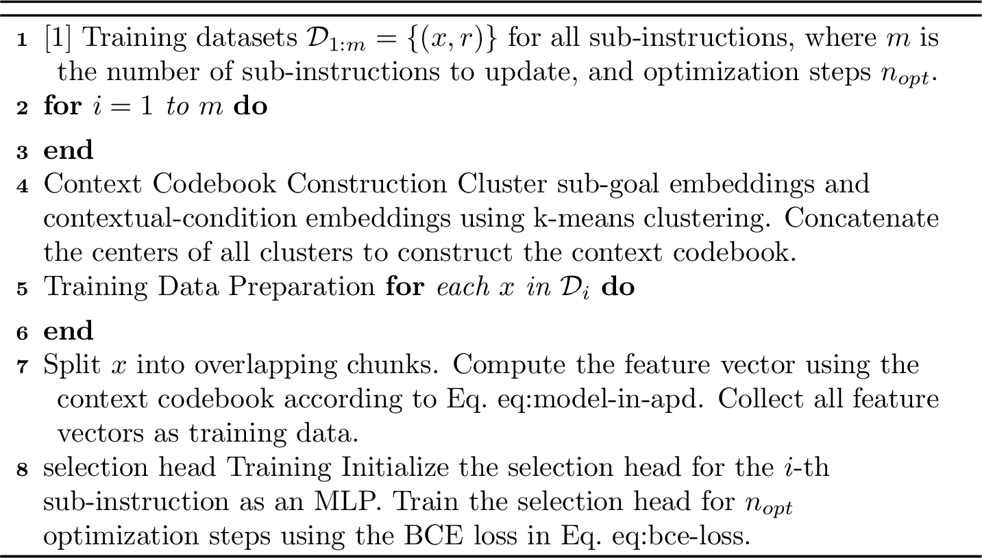
The detailed training process is described in Alg. 9.
10.0.0.1 Construction and application of context code book.
The step-goal describes the objective the next reasoning step is intended to achieve, while the contextual condition captures the most relevant information for generating that step. Together, they are the key factors determining whether a sub-instruction is applicable to a given reasoning state. During data collection, since each instruction may be applied across multiple reasoning states, we collect the corresponding step-goal and contextual conditions and compute their embeddings. We then cluster these embeddings and use the centroid of each cluster as a context codebook. In this way, context codebooks serve as representative embeddings of similar step-goal and contextual conditions. Each selection head maintains an individual context codebook to identify the information most relevant to its corresponding sub-instruction.
The context codebooks are used to identify relevant information in the reasoning state. Specifically, we first split the reasoning state into overlapping chunks and compute embeddings for each chunk. We then compute the maximum cosine similarity between each context codebook and the chunk embeddings: \[\mathbf{m}_a(x) \;=\; [s_{a1}, s_{a2}, \ldots, s_{an}], \qquad s_{ai} \;=\; \max_{j \in [1, T]} \mathrm{cos}(\mathbf{q}_{ai}, \mathbf{c}_j), \label{eq:model-in-apd}\tag{18}\] where \(\mathbf{m}_a(x)\) denotes the feature vector, \(\mathbf{q}_{ai}\) and \(\mathbf{c}_j\) represent the \(i\)-th context prototype and the \(j\)-th chunk embedding, respectively, \(T\) is the number of chunks, and \(n\) is the number of context prototypes.
Intuitively, the maximum cosine similarity captures whether information relevant to a given context codebook is present in the reasoning state: a higher similarity indicates stronger evidence of its presence. Thus, Eq. 18 encodes the presence of different step-goal and condition patterns into a fixed-dimensional feature vector, which is then used by the selection head to determine whether a sub-instruction should be applied.
10.0.0.2 Discussion with Q-learning.
In LLM reasoning tasks, supervision is typically limited to the correctness of the final solution, resulting in sparse and delayed rewards. This makes it challenging to reliably estimate the contribution of individual intermediate actions. Value-based approaches, such as Q-learning, require estimating the expected reward of each action under a given reasoning state, which in practice relies on sufficient rollout samples. When the number of observations per sub-instruction is limited, accurately estimating such values becomes difficult and may suffer from high variance. In our setting, each sub-instruction is applied under diverse reasoning states, and only a small number of samples are available for each instruction–state pair. As a result, value estimation for individual instructions can be unreliable. In extreme cases, if the observed trajectories associated with a given instruction all lead to correct final answers, a value-based model may assign uniformly high values, failing to distinguish the conditions under which the instruction is truly applicable. Instead of explicitly estimating action values, our approach directly approximates closed form optimal policy over instructions using binary correctness signals, avoiding per-action value estimation under limited samples.
10.0.0.3 Discussion with ColBERT.
ColBERT [53] measures document relevance to a query by summing the maximum similarity between each context codebook and the document vectors, where both are encoded by a BERT encoder. We use the cluster centers as context codebooks and follow the same idea that identify key information from one sequence by maximum similarity. Different from ColBERT [53], we retain the full sequence of maximum similarities between the context codebooks and the document vectors as the input representation, this indicates a combination of different queries.
10.0.0.4 Method for preventing overfitting.
Since only a limited amount of data is collected for each sub-instruction, the selection heads may overfit to the training data and fail to generalize to new cases. To mitigate this issue, we adopt the following strategies:
Cross-instruction pretraining. For a target sub-instruction, we first collect data from other instructions with similar sub-goals. A model is then trained on this combined dataset using the binary cross-entropy loss, which encourages the model to learn more diverse patterns for instruction selection. Finally, we fine-tune the classification layer on the training data of the target sub-instruction while keeping the remaining parameters fixed.
Input dropout. During training, we apply dropout to the input dimensions of the selection heads to prevent certain dimensions from dominating the prediction. This regularization encourages the model to rely on more robust features and improves generalization to unseen conditions.
Regularization techniques. In practice, we train multiple selection heads and average their predicted probabilities to obtain a more robust estimate. We additionally employ early stopping and weight decay to further reduce the risk of overfitting to the training data.
10.0.0.5 Preventing catastrophic forgetting.
During test time, samples arrive sequentially, and the training data for each selection head is incrementally accumulated. As a result, the selection heads must be updated to incorporate newly acquired knowledge. However, updating the model on new data can lead to a significant degradation in performance on previously seen data, a phenomenon known as catastrophic forgetting [54]. To mitigate this issue while preventing extra complexity, we adopt a simple rehearsal strategy: we retain all previously collected data and train the selection heads jointly on both new and past data.
11 Additional experiments↩︎
11.1 Comparison with more baseline methods↩︎
ll >cc >cc Method type & Method & AIME 2024 & AIME 2025
& Zero-shot CoT [30] & 46.67 & 46.67
& AoT [55] & 63.33 & 50.00
& BoT [5] & 50.00 & 40.00
& DC (w/ coding) [9] & 63.33 & 60.00
& DC (w/o coding) [9] & 46.67 & 33.33
& CoT-SC [2] & 56.67 & 53.33
& ToT [3] & 50.00 & 53.33
& rStar [4] & 56.67 & 53.33
& DORA [20] & 50.00 & 30.00
& Our method & 66.67 & 60.00
To further evaluate the effectiveness of our method, we compare it against a broad range of baselines on the AIME 2024 and AIME 2025 datasets using the GPT-4.1-mini model. The baselines include: Prompt-based methods guide LLM reasoning by designing effective prompts.
Zero-shot CoT [30] elicits reasoning by simply adding the prefix “Let’s think step by step.”.
Atom of Thoughts (AoT) [55] models reasoning as a Markovian process, where each state corresponds to a self-contained subproblem.
Memory-based methods accumulate reusable knowledge and strategies from prior reasoning experiences and leverage memory to guide LLMs in solving new problems.
Buffer of Thoughts (BoT) [5] distills reasoning templates from past experiences and retrieves the most relevant templates to guide reasoning on new problems.
Dynamic CheatSheet (DC) [9] distills and refines reusable strategies from prior experiences, and applies the most relevant strategy to solve new problems.
Test-time scaling methods allocate additional computation during inference to further improve reasoning performance.
Self-Consistency (SC) [2] aggregates multiple reasoning trajectories to produce more reliable predictions.
Tree-of-Thoughts (ToT) [3] introduces a structured reasoning framework that enables LLMs to flexibly explore and expand multiple reasoning states, improving their problem-solving capabilities.
rStar [4] explores reasoning states using human-like actions within a Monte Carlo Tree Search (MCTS) framework, and selects trajectories based on mutual consistency.
DORA [20] adaptively allocates rollout budgets based on PRM scores and trajectory similarity, assigning more computation to reasoning states that exhibit lower similarity and higher PRM scores.
We compare all methods in terms final accuracy; results are reported in Table ¿tbl:tab:full-exp?. Compared to other test-time scaling approaches, MILES achieves higher accuracy, demonstrating the effectiveness of its memory construction and selection strategy.
DORA adaptively allocates rollouts to promising reasoning states, but performs worse than other methods, suggesting that PRMs may be unreliable for API-based models. In contrast, MILES improves performance without relying on external PRMs, highlighting its robustness.
Among memory-based methods [5], [15], DC achieves strong performance when coding is enabled, but its performance degrades substantially without coding. MILES achieves superior performance by leveraging additional computation for training-data collection and memory-guided tree search.
Across all compared methods, MILES consistently outperforms the baselines on both datasets, demonstrating the effectiveness and robustness of our method.
11.2 Component ablation with more models↩︎
| Dataset | Layer 1 | Layer 2 | GPT-4.1-mini | Qwen3-30B-Instruct |
|---|---|---|---|---|
| AIME 2024 | 60.00 | 83.33 | ||
| 63.33 | 83.33 | |||
| 66.67 | 86.67 | |||
| AIME 2025 | 53.33 | 70.00 | ||
| 53.33 | 70.00 | |||
| 60.00 | 73.33 |
In addition to the ablation study in Section [sec:ablation], we further evaluate our method across different LLMs, including GPT-4.1-mini and Qwen3-30B-Instruct, on the AIME 2024 and AIME 2025 datasets. Results are reported in Table 3.
Our method consistently improves performance across different models and datasets, demonstrating its effectiveness and robustness. We also observe that the performance of Qwen3-30B-Instruct is already close to saturation.
11.3 Ablation of summarization parameters↩︎
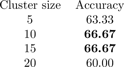
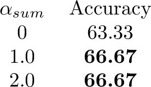
To evaluate the effect of our summarization method, we study two hyperparameters: (1) \(\alpha_{\text{sum}}\), which balances the similarities between step-goal embeddings and step embeddings; and (2) the minimum cluster size, which controls the level of abstraction, as only clusters whose size exceeds this threshold are summarized into sub-instructions. Both are evaluated on AIME 2024 with GPT-4.1-mini in Tables [tbl:tab:cluster-alpha] and ¿tbl:tab:cluster-size?.
Both hyperparameters show same robustness pattern. Accuracy is stable across a moderate range and only degrades at the extremes. For \(\alpha_{\text{sum}}\) (Table [tbl:tab:cluster-alpha]), values in \([1.0, 2.0]\) all remains 66.67%; only setting \(\alpha_{\text{sum}} = 0\), which discards step-goal similarity entirely during clustering. For the minimum cluster size (Table ¿tbl:tab:cluster-size?), values in \([10, 15]\) also remains stable; cluster sizes that are too small (e.g., 5) produce overly specific sub-instructions and drop accuracy, while cluster sizes that are too large (e.g., 20) produce overly generic sub-instructions and also drop. In practice we use \(\alpha_{\text{sum}} = 1.0\) and a minimum cluster size in \([10, 15]\) across all experiments (Appendix 14) without further tuning.
11.4 Impact of effective threshold↩︎
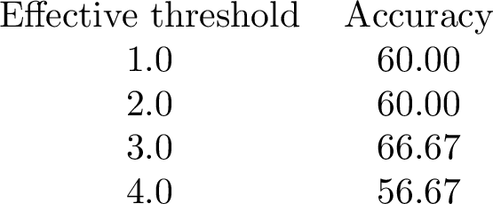
The effective threshold \(\alpha_{\text{eff}}\) controls how broadly a sub-instruction is allowed to be applied: a larger threshold allows more diverse application contexts (and more diverse training trajectories) but raises the risk of applying a sub-instruction to states it does not fit. We evaluate the effect of \(\alpha_{\text{eff}} \in \{1.0, 2.0, 3.0, 4.0\}\) on AIME 2025 with GPT-4.1-mini.
Table ¿tbl:tab:eff-thd? shows that MILES is largely insensitive to \(\alpha_{\text{eff}}\) over a wide range: accuracy stays at or above 60.00% for \(\alpha_{\text{eff}} \in \{1.0, 2.0, 3.0\}\), peaking at at 3.0, and only degrades to 56.67% at the extreme value 4.0, where overly broad applicability introduces irrelevant sub-instructions. In our experiments we use \(\alpha_{\text{eff}} = 2.0\) for math datasets (Appendix 14) without further tuning.
11.5 Ablation on context codebook↩︎
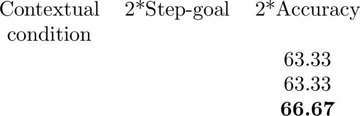
The context codebook in Layer 2 is built by clustering embeddings of contextual conditions and sub-goals (Section [sec:mem-rs]); we ablate the contribution of these two components on AIME 2024 with GPT-4.1-mini. Removing either component drops accuracy by 3.34 points (66.67% \(\to\) 63.33%), while combining both yields the best result (Table [tbl:tab:codebook]), supporting the assumption that a sub-instruction’s applicability is jointly determined by what the next step should achieve i.e., step-goal and what context the current state provides.
11.6 Ablation on number of candidate sub-instructions↩︎
| Candidate number | Accuracy |
|---|---|
| 8 | 53.33 |
| 16 | 60.00 |
| 24 | 60.00 |
R0.4
In memory-guided tree search, Layer 1 first retrieves candidate sub-instructions based on sub-goal similarity, which are then reranked by Layer 2 selection. We study the effect of the number of Layer 1 candidates on AIME 2025 with GPT-4.1-mini; results are reported in Table 4. Performance drops when too few candidates are retrieved (8 candidates), but remains stable with larger candidate sets (16 and 24), indicating that Layer 2 selection effectively identifies useful sub-instructions from the retrieved candidates. In all experiments, we use 16 candidates without tuning this hyperparameter.
11.7 Effect of selected sub-instructions↩︎
To validate that the sub-instructions selected during memory-guided tree search actually help, we compare, under matched reasoning states, the accuracy of reasoning trajectories that include steps guided by a selected sub-instruction against trajectories generated without such guidance. Experiments are conducted on all six benchmarks with GPT-4.1-mini and GPT-4.1; Table 5 reports the resulting accuracy improvement in percentage points.
| Dataset | Accuracy improvement | |
|---|---|---|
| 2-3 | GPT-4.1-mini | GPT-4.1 |
| MATH-500 | 6.48 | 2.23 |
| AIME 2024 | 10.80 | 3.77 |
| AIME 2025 | 9.12 | 2.31 |
| GPQA-Diamond | 4.36 | 3.21 |
| MMLU-Pro Physics | 4.12 | 8.73 |
| MMLU-Pro Engineering | 0.63 | 3.87 |
As shown in Table 5, applying selected sub-instructions consistently improves reasoning performance across all 12 dataset-model cells (range 0.63–10.80 points), with the largest gains on the harder math benchmarks. This confirms that the sub-instructions retrieved and reranked by our two-layer mechanism are effective at steering the LLM toward correct final answers.
12 Efficiency discussion↩︎
12.1 Reducing time delay via parallel data collection.↩︎
Our method relies on MCTS with multiple rollouts to collect teacher trajectories for training the selection heads, which can be time-consuming. To mitigate this overhead, we leverage parallel computation to reduce data collection latency.
Specifically, after the initial rollouts in MCTS, we estimate a pseudo ground-truth answer via majority voting and check for consistency across rollouts. If the answers are consistent, the LLM can directly return the final prediction, as additional data collection does not affect the outcome. In this case, trajectory collection can proceed asynchronously in the background, while the system handles new queries in parallel. If the answers are inconsistent, we instead invoke memory-guided tree search to continue reasoning and determine the final answer.
12.2 Applying KV-cache to reduce computation.↩︎
During both MCTS and memory-guided tree search, new branches are expanded from existing reasoning steps by prompting the LLM with the question, previous steps, and a selected sub-instruction to generate the next reasoning step. For open-source LLMs, the KV cache of previously processed tokens can be reused. As a result, the model avoids recomputing representations for earlier tokens, significantly reducing the computational cost of tree search.
13 Broader impact↩︎
We propose a framework that learns to select sub-instructions at test time to improve reasoning performance. Our method does not require curated training datasets or process reward models (PRMs), enabling effective learning under limited data. Moreover, the memory construction process incrementally incorporates new sub-instructions as experience accumulates, allowing the system to adapt to diverse scenarios by updating memory rather than modifying LLM parameters.
As our approach relies on textual memory that is compatible across different LLMs, it enables knowledge transfer across models. In particular, trajectories collected from stronger models can be used to train selection policies for weaker models, potentially improving accessibility to high-quality reasoning capabilities without requiring large-scale training resources. Importantly, the teacher model does not need to be uniformly stronger across all domains. In specific areas, a smaller but more specialized model can provide high-quality trajectories to train selection policies for other models, enabling flexible and domain-specific knowledge transfer.
However, since the selection policy is learned from collected trajectories, it may inherit biases or errors present in the data, potentially leading to misleading or suboptimal outputs. Additionally, the accumulation of memory over time may amplify such biases if not properly controlled. To mitigate these risks, the use of textual memory allows for transparent inspection, as well as LLM-based verification and feedback. Future work may explore mechanisms for monitoring, filtering, and refining memory and selection policies through self-checking or external supervision.
14 Implementation details↩︎
14.1 MCTS details↩︎
The detailed hyperparameters of MCTS are reported in Table 6. For more complex datasets, such as AIME 2024 and AIME 2025, we use greater search depth and more rollouts to collect training trajectories, while keeping the same hyperparameters for other datasets. The exploration constant \(C\) in Eq. 16 is set to 1.0 across all experiments.
| Dataset | Rollouts | Depth | Children Nodes | \(C\) |
|---|---|---|---|---|
| Math-500 | 20 | 4 | 3 | 1.0 |
| AIME 2024 | 40 | 5 | 3 | 1.0 |
| AIME 2025 | 40 | 5 | 3 | 1.0 |
| GPQA-Diamond | 20 | 4 | 3 | 1.0 |
| MMLU-Pro Physics | 20 | 4 | 3 | 1.0 |
| MMLU-Pro Engineering | 20 | 4 | 3 | 1.0 |
14.2 Memory construction details↩︎
When clustering (step, sub-goal) embeddings, instead of fixing the number of clusters in k-means, we impose a minimum cluster size to ensure that sub-instructions are summarized from sufficiently diverse reasoning steps, resulting in more reusable abstractions. Specifically, we set the minimum cluster size in the range of \([10, 20]\), depending on the similarity among queries within each dataset.
For math tasks, we set the effective threshold to 2.0, as sub-instructions tend to generalize well across queries. In contrast, for academic tasks, we use a lower threshold in the range of \([1.0, 1.5]\), since sub-instructions are less transferable across different queries.
14.3 Training details↩︎
We use a 3-layer MLP with 16 hidden units as the selection head. For each sub-instruction, we train 10 independent classifiers and average their predicted application probabilities to improve robustness. We periodically update the classifiers during test-time processing: after every 2 questions, and whenever the number of training trajectories increases by 20. For smaller datasets such as AIME 2024 and AIME 2025, we instead update the selection heads after each question.
The context prototypes correspond to the cluster centers obtained from embeddings of contextual conditions and step-goals. We set the number of context prototypes (i.e., the number of clusters in k-means clustering) to \(\min(Nc_i \cdot 0.2, 512)\), where \(Nc_i\) denotes the number of application cases for the \(i\)-th sub-instruction. The number of context prototypes increases gradually as the application cases become more diverse. We cap the maximum number at 512 to avoid overly complex context codebooks while maintaining clustering efficiency.
14.4 Memory guided tree search details↩︎
In our method, the application of memory-guided tree search is determined by the majority-answer proportion, i.e., answer consistency. Since different models exhibit different levels of answer consistency, we set the consistency threshold slightly lower than the zero-shot CoT accuracy measured on a small validation subset. We set the number of routing rollouts to 10 for all experiments. The detailed hyperparameters of memory-guided tree search are reported in Table 7. For more complex datasets, such as AIME 2024 and AIME 2025, we use greater search depths and more rollouts to enable broader application of sub-instructions during reasoning.
The parameter \(\beta_{\text{c2f}}\) in Eq. 3 controls the balance between selection and semantic relevance. We set \(\beta_{\text{c2f}}=0.0\) for math tasks, so that selection is determined solely by the selection heads, and use values in the range \([0.4, 0.6]\) for academic tasks to place greater weight on semantic relevance.
| Dataset | Stage | Rollout per stage | Candidate instructions | \(\beta_{\text{c2f}}\) |
|---|---|---|---|---|
| Math-500 | 5 | 4 | 16 | 0.0 |
| AIME 2024 | 6 | 4 | 16 | 0.0 |
| AIME 2025 | 6 | 4 | 16 | 0.0 |
| GPQA-Diamond | 5 | 4 | 16 | 0.4-0.6 |
| MMLU-Pro Physics | 5 | 4 | 16 | 0.4-0.6 |
| MMLU-Pro Engineering | 5 | 4 | 16 | 0.4-0.6 |
14.5 Decoding details↩︎
For all experiments using GPT-4.1-mini and GPT-4.1, we use the OpenAI API service. The decoding temperature is set to 0.0 for all experiments. The maximum response length is determined according to task complexity, ranging from 2048 to 16384 tokens. For
experiments with GPT-4.1-mini, we use the GPT-4.1-mini-2025-04-14 checkpoint.
For experiments using open-source models, we employ the vLLM framework [56] for local decoding and the OpenRouter API for online decoding. For all Qwen3 models, we follow the decoding settings described in the original paper [28]. For the GPT-OSS-20B model, we set the decoding temperature to 1.0 for all experiments.
All experiments use text-embedding-3-small from the OpenAI API service for embedding computation. The embedding dimension is fixed at 1536 across all experiments.
15 Computation resources and assets↩︎
For experiments using API-based models, we train the selection heads on a single RTX 3090 GPU and access the models via LiteLLM https://docs.litellm.ai/. For open-source models, we either (1) deploy the models locally on a server with 8 A100 GPUs, or (2) access inference services through OpenRouter https://openrouter.ai/.
Open-sourced model URLs:
Qwen3-30B-Instruct: https://huggingface.co/Qwen/Qwen3-30B-A3B-Instruct-2507.
Qwen3-4B-Instruct: https://huggingface.co/Qwen/Qwen3-4B-Instruct-2507.
GPT-OSS-20B: https://huggingface.co/openai/gpt-oss-20b.
Dataset URLs:
AIME datasets: https://artofproblemsolving.com/wiki/index.php/AIME_Problems_and_Solutions.
MATH-500: https://huggingface.co/datasets/HuggingFaceH4/MATH-500.
GPQA-Diamond: https://huggingface.co/datasets/fingertap/GPQA-Diamond.
MMLU-Pro: https://huggingface.co/datasets/TIGER-Lab/MMLU-Pro.
16 Case study↩︎
To illustrate the effectiveness of sub-instructions, we present two case studies from the algebra and geometry categories of MATH-500 during memory-guided tree search. For each case, we first show the response generated by Zero-shot CoT, followed by the response obtained by applying a selected sub-instruction at an intermediate reasoning step, together with the corresponding sub-instruction. Selected sub-instructions are highlighted in red, while shared responses between the two reasoning trajectories are highlighted in purple.
16.1 Algebra case↩︎
Question: Let \(x,\) \(y,\) and \(z\) be positive real numbers such that \(xyz = 2.\) Find the minimum
value of \(x^4 + 4y^2 + 4z^4\).
Zero-shot CoT:
Step 1: We can apply the AM-GM inequality to the terms \(x^4\), \(2y^2\), \(2y^2\), \(2z^4\), and \(2z^4\) to relate their sum to their product, taking into account the constraint \(xyz = 2\).
Step 2: Let’s rewrite the expression as follows: \[x^4 + 4y^2 + 4z^4 = x^4 + 2y^2 + 2y^2 + 2z^4 + 2z^4 \notag\] Now, we have five terms: \(x^4\), \(2y^2\),
\(2y^2\), \(2z^4\), \(2z^4\).
Step 2: By the AM-GM inequality, we have \[x^4 + 2y^2 + 2y^2 + 2z^4 + 2z^4 \geq 5 \left(x^4 \cdot (2y^2)^2 \cdot (2z^4)^2\right)^{1/5}. \notag\]
Step 3: Let’s simplify the product inside the root: \[x^4 \cdot (2y^2)^2 \cdot (2z^4)^2 = x^4 \cdot 4y^4 \cdot 4z^8 = 16 x^4 y^4 z^8. \notag\]
Step 4: Recall the constraint \(xyz = 2\). We can write \(z = \frac{2}{xy}\), so \[z^8 = \left(\frac{2}{xy}\right)^8 = \frac{256}{x^8 y^8}. \notag\] Thus,
\[16 x^4 y^4 z^8 = 16 x^4 y^4 \cdot \frac{256}{x^8 y^8} = 16 \cdot 256 \cdot x^4 y^4 / (x^8 y^8) = 4096 \cdot \frac{1}{x^4 y^4}. \notag\]
Step 5: Substitute this back into the AM-GM inequality: \[x^4 + 4y^2 + 4z^4 \geq 5 \left(4096 \cdot \frac{1}{x^4 y^4}\right)^{1/5} = 5 \cdot 4096^{1/5} \cdot (x^4 y^4)^{-1/5}. \notag\]
Step 6: Compute \(4096^{1/5}\). Since \(4096 = 2^{12}\), \(4096^{1/5} = 2^{12/5} = 2^{2.4}\).
Step 7: Now, let’s try to achieve equality in AM-GM, which occurs when all terms are equal: \[x^4 = 2y^2 = 2y^2 = 2z^4 = 2z^4. \notag\] So \(x^4 = 2y^2 = 2z^4\).
Step 8: Set \(x^4 = 2y^2\) and \(x^4 = 2z^4\). Then \(y^2 = \frac{x^4}{2}\) and \(z^4 = \frac{x^4}{2}\), so \(z^2 = \left(\frac{x^4}{2}\right)^{1/2} = \frac{x^2}{\sqrt{2}}\).
Step 9: Now, use the constraint \(xyz = 2\): \[x \cdot y \cdot z = 2. \notag\] Recall \(y = \frac{x^2}{\sqrt{2}}\) and \(z =
\frac{x^2}{\sqrt{2}}\), so \[x \cdot \frac{x^2}{\sqrt{2}} \cdot \frac{x^2}{\sqrt{2}} = 2 \implies x \cdot \frac{x^4}{2} = 2 \implies \frac{x^5}{2} = 2 \implies x^5 = 4 \implies x = 4^{1/5} = 2^{2/5}. \notag\]
Step 10: Now, \(y = \frac{x^2}{\sqrt{2}} = \frac{(2^{2/5})^2}{\sqrt{2}} = \frac{2^{4/5}}{2^{1/2}} = 2^{4/5 - 1/2} = 2^{(8-5)/10} = 2^{3/10}\).
Similarly, \(z = 2^{3/10}\).
Step 11: Now, compute the minimum value: \[x^4 + 4y^2 + 4z^4 = (2^{2/5})^4 + 4(2^{3/10})^2 + 4(2^{3/10})^4. \notag\]
Calculate each term: - \(x^4 = (2^{2/5})^4 = 2^{8/5}\) - \(y^2 = (2^{3/10})^2 = 2^{6/10} = 2^{3/5}\) - \(z^4 = (2^{3/10})^4 = 2^{12/10} = 2^{6/5}\)
So, \[x^4 + 4y^2 + 4z^4 = 2^{8/5} + 4 \cdot 2^{3/5} + 4 \cdot 2^{6/5} \notag\]
Step 12: This is the minimum value. Thus, the answer is \(\boxed{2^{8/5} + 4 \cdot 2^{3/5} + 4 \cdot 2^{6/5}}\)
Apply sub-instruction
<Sub-instruction>
Rewrite or simplify algebraic expressions or equations by substituting variables, factoring, or using properties of roots and exponents to transform them into more manageable forms.
</Sub-instruction>
Step 2: Substitute \(z = \frac{2}{xy}\) into the expression to rewrite it as \(x^4 + 4y^2 + 4\left(\frac{2}{xy}\right)^4\).
Step 3: Simplify the expression: \[x^4 + 4y^2 + 4\left(\frac{2}{xy}\right)^4 = x^4 + 4y^2 + 4 \cdot \frac{16}{x^4y^4} = x^4 + 4y^2 + \frac{64}{x^4y^4} \notag\]
Step 4: Let \(a = x^4\) and \(b = y^2\), so \(x = a^{1/4}\), \(y = b^{1/2}\), and \(z =
\frac{2}{xy} = \frac{2}{a^{1/4}b^{1/2}}\).
Step 5: Substitute these into the constraint \(xyz = 2\): \[x y z = a^{1/4} b^{1/2} \cdot \frac{2}{a^{1/4} b^{1/2}} = 2 \notag\] So the constraint is satisfied for all positive \(a, b\).
Step 6: The expression to minimize is: \[a + 4b + \frac{64}{ab^2} \notag\]
Step 7: Let’s use symmetry and try \(a = 2b\) (since the terms \(a\) and \(b\) appear with different powers, but the last term is symmetric in \(a\) and \(b^2\)). Set \(a = k b\), so: \[a + 4b + \frac{64}{ab^2} = k b + 4b + \frac{64}{k b^3} \notag\] Let’s try \(k = 2\): \[2b + 4b + \frac{64}{2b^3} = 6b + \frac{32}{b^3} \notag\] Now, minimize \(6b + \frac{32}{b^3}\) for \(b >
0\).
Step 8: Take the derivative with respect to \(b\) and set to zero: \[\frac{d}{db}\left(6b + \frac{32}{b^3}\right) = 6 - \frac{96}{b^4} = 0 \implies 6 = \frac{96}{b^4} \implies b^4 = 16 \implies b
= 2 \notag\]
Step 9: Substitute \(b = 2\) back: \[6b + \frac{32}{b^3} = 6 \times 2 + \frac{32}{8} = 12 + 4 = 16 \notag\]
Step 10: Recall \(a = 2b = 4\), so \(x^4 = 4 \implies x = \sqrt{2}\), \(y^2 = 2 \implies y = \sqrt{2}\), and \(z = \frac{2}{xy} =
\frac{2}{2} = 1\).
Step 11: Check the constraint: \(xyz = \sqrt{2} \cdot \sqrt{2} \cdot 1 = 2\), which is satisfied.
Step 12: Compute the original expression: \[x^4 + 4y^2 + 4z^4 = 4 + 4 \times 2 + 4 \times 1 = 4 + 8 + 4 = 16 \notag\] Final answer:
In the Zero-shot CoT response, the LLM attempts to solve the problem using the AM-GM inequality. However, this formulation leads to complicated computations and ultimately produces an incorrect answer. In contrast, the selected sub-instruction guides the LLM to first transform the expression into a more manageable form. As a result, the LLM simplifies the formula and successfully reaches the correct answer.
16.2 Geometry case↩︎
Question: Quadrilateral \(ABCD\) is a square with area 16 square inches. The figure represents the pieces of a Chinese tangram in which all the triangles are isosceles and piece "e” is a square. What is the area of the gray piece, in square inches?
Figure 10:  .
.
Zero-shot CoT:
Step 1: Since the area of square \(ABCD\) is \(16\) square inches, its side length is \(\sqrt{16} = 4\)
inches.
Step 2: The tangram divides the square into 7 pieces: 5 triangles, 1 parallelogram, and 1 small square (piece "e"). All triangles are isosceles right triangles, and piece "e" is a square.
Step 3: The gray piece in the diagram is the small triangle at the bottom right, adjacent to \(C\) and below piece "e". We need to find its area.
Step 4: Let’s analyze the construction. The classic tangram divides the square into the following pieces (by area, as fractions of the whole square):
- 2 large triangles (each \(\frac{1}{4}\) of the area)
- 1 medium triangle (\(\frac{1}{8}\))
- 2 small triangles (each \(\frac{1}{16}\))
- 1 square (\(\frac{1}{8}\))
- 1 parallelogram (\(\frac{1}{8}\))
Step 5: The gray triangle is one of the two smallest triangles, each with area \(\frac{1}{16}\) of the total area.
Step 6: Since the total area is 16 square inches, the area of the gray piece is \(16 \times \frac{1}{16} = 1\) square inch.
Final answer:
Apply sub-instruction
<Sub-instruction>
Calculate the area of a triangle with sides \(a\), \(b\), and \(c\) by first finding the semi-perimeter \(s = \frac{a+b+c}{2}\), then applying Heron’s formula: \(A = \sqrt{s(s-a)(s-b)(s-c)}\).
</Sub-instruction>
Step 3: To find the area of the gray triangle with vertices at \((2,0)\), \((4,0)\), and \((4,2)\), first compute the side lengths: \(a = 2\) (from \((2,0)\) to \((4,0)\)), \(b = 2\) (from \((4,0)\) to \((4,2)\)), and \(c = \sqrt{(4-2)^2 + (2-0)^2} = \sqrt{4+4} = 2\sqrt{2}\) (from \((2,0)\) to \((4,2)\)).
Step 4: The triangle is a right triangle with legs of length \(2\) (from \((2,0)\) to \((4,0)\) and from \((4,0)\) to \((4,2)\)), so its area is \(\frac{1}{2} \times 2 \times 2 = 2\) square inches.
Step 5: Therefore, the area of the gray piece is square inches.
In the Zero-shot CoT response, the LLM directly estimates the area of the gray region based on the partition of the square. However, it identifies the wrong triangle, which leads to an incorrect final answer. In contrast, the selected sub-instruction guides the LLM to compute the area of the gray region using Heron’s formula. Consequently, the LLM first computes the lengths of the edges of the gray region in the following step. Although the LLM does not explicitly apply Heron’s formula afterward, the computed edge lengths help it derive the correct area.
From the above cases, we observe that the selected sub-instructions guide the LLM toward more promising reasoning directions, ultimately leading to correct final answers. These results suggest that our method effectively achieves the objective of selecting appropriate sub-instructions to maximize the probability of generating correct solutions, demonstrating the effectiveness of our approach.
17 All prompts↩︎
To ensure generalizability across tasks, we use a unified set of prompts for all experiments. To maintain compatibility with smaller models such as Qwen3-30B-Instruct and GPT-OSS-20B, we keep the prompts simple and straightforward.
Generate step-goal. This prompt generates a step-goal for the next reasoning step based on the current reasoning state. The resulting step-goal is used to select a sub-instruction by computing cosine similarity between its embedding and the stored sub-goals. The selected sub-instruction then guides the generation of the next reasoning step.
Instruction: Given the Question and Reasoning so far, output the immediate next-step objective that directly contributes toward achieving the final goal based on current progress. Respond in one sentence only.
Question:
<question>
Reasoning so far:
<reasoning so far>
Generate next step with sub-instruction. This prompt guides the LLM to generate the next reasoning step conditioned on the selected sub-instruction and the current reasoning state. In both MCTS and memory-guided tree search, generating the next reasoning step corresponds to expanding a new branch from the existing reasoning state.
Instruction: Apply the given instruction to generate the NEXT reasoning step only.
- Output a single step, one sentence.
- Be precise. Use exact numbers, variables, or terms from the question and prior steps.
- Do not restate irrelevant details.
- Keep it in the same style as the previous steps.
- If the reasoning is complete, present the final answer as (
boxed{x}), where X is the correct answer.
Question:
<question>
Reasoning so far:
<reasoning so far>
Relevant instruction:
<relevant instruction>
Generate next step without sub-instruction. When no sub-instruction is selected, we prompt the LLM to generate the next reasoning step to achieve the given step-goal. The resulting (step-goal, reasoning step) pair is then stored for summarizing new sub-instructions.
Instruction: Generate the Next reasoning step that best fulfills the given Objective of the next step in the context of the Question and Reasoning so far.
- Output a single step, one sentence.
- Be precise. Use exact numbers, variables, or terms from the question and prior steps.
- Do not restate irrelevant details.
- Keep it in the same style as the previous steps.
- If the reasoning is complete, present the final answer choice as (
boxed{x}), where X is the correct answer.
Question:
<question>
Reasoning so far:
<reasoning so far>
Objective of the next step:
<objective of the next step>
Complete reasoning. This prompt directly asks the LLM to complete the reasoning from the current reasoning state, corresponding to the simulation phase in MCTS. In memory-guided tree search, we perform completion after each expansion. Specifically, after applying a sub-instruction to generate a new reasoning step, we prompt the LLM to complete the remaining reasoning and produce the final solution.
Instruction: You are given a question and a partially completed reasoning chain. Continue the reasoning step by step, each step starts with ‘Step \(i\):’, where \(i\) is the step number, until the solution is complete. Do not restart from the beginning.
Present the final answer as (
boxed{x}), where X is the correct answer.
Question:
<question>
Reasoning so far:
<reasoning so far>
Summarize sub-instructions. This prompt asks the LLM to extract common reasoning patterns from multiple similar reasoning steps and summarize them into a sub-instruction. The resulting sub-instruction is then used to guide the generation of new reasoning steps when selected.
Instruction: You are given several reasoning steps that are semantically similar.
Your task is to summarize them into a general instruction that captures the shared logic or operation behind these steps.
Guidelines:
- Abstract away task-specific numbers or entities (replace them with variables or placeholders).
- Keep the instruction short and action-oriented (like a recipe step).
- If there are small differences across the steps, generalize to a pattern that covers them.
- Output only one generalized instruction.
Reasoning Steps:
<Reasoning Steps>
Format:
<general_instruction>
[one-sentence generalized instruction here, using variables or placeholders if needed]
</general_instruction>
Identify contextual conditions. This prompt extracts the contextual conditions for a reasoning step from the question and preceding responses. The extracted conditions are used to build a codebook that identifies the most relevant context for applying the corresponding sub-instruction.
Instruction: Try to identify the INPUT CONDITIONS for the NEXT reasoning step only (not the whole solution) from Question and the Reasoning so far.
- Output the identified INPUT CONDITIONS only.
Question:
<question>
Reasoning so far:
<reasoning so far>
Next reasoning step:
<next reasoning step>