General Incomplete Multimodal Learning via Dynamic Quality Perception
January 01, 1970
Abstract
Multimodal learning robust to missing modalities is essential for real-world applications. Existing methods mainly focus on inter-modality missing, where entire modalities are absent, while overlooking intra-modality degradation, where modalities are present but severely corrupted. In practice, these two types of missing often coexist, making existing approaches ineffective. To address this limitation, we propose General Incomplete Multimodal Learning (GIML), a unified framework that simultaneously handles both inter-modality missing and intra-modality degradation through dynamic quality perception. Specifically, GIML models heterogeneous missing patterns as continuous modality information degradation, enabling degradation-aware adaptive fusion. To achieve reliable quality perception, we introduce a Noise-aware Quality Estimator that learns the mapping from corrupted features to noise intensity through controlled noise injection. Furthermore, we propose a Noise–Semantic Decoupled module that separates semantic information from noise interference. This improves robustness and generalization to unseen corruption patterns. Extensive experiments across datasets with diverse modality types demonstrate the effectiveness and generality of GIML. Code is available at: https://github.com/Yu-Five/GIML.
Keywords: Multimodal learning, Dynamic quality perception, Modality missing
1 Introduction↩︎
Multimodal learning has achieved strong performance across many vision tasks [1]–[3]. However, most existing methods assume that all modalities are available during training and inference. This assumption often fails in practice due to device limitations [4], [5] or challenging operating conditions [6], [7]. Such incompleteness can significantly harm model performance and robustness, motivating the study of incomplete multimodal learning.
Existing approaches generally fall into two categories: imputation-based and joint representation-based methods. Imputation-based methods reconstruct missing modalities from available ones at the input [4], [8], [9] or representation level [10]–[17]. While this type of method is straightforward, their performance heavily depends on reconstruction quality and errors can propagate to downstream tasks. Thus, joint representation-based methods instead learn unified embeddings from different modality combinations without explicit reconstruction. They capture the shared feature for all possible input modality combinations to address the incomplete multimodal learning issue [18]–[22].
Despite the success of existing methods, most focus on inter-modality missing, where entire modalities are absent. In practice, however, modality incompleteness also occurs within modalities, where inputs are present but corrupted by noise. Recent works such as T2DR [23] and TMDC [24] attempt to address this issue, but they treat intra-modality corruption and inter-modality missing as two separate problems and handle them sequentially. This could encounter the optimization conflicts across stages, resulting in sub-optimal performance. Moreover, they are typically designed for specific intra-modal corruption, such as Gaussian degradation. This limits their robustness to unseen missing patterns.
To address these limitations, we propose General Incomplete Multimodal Learning (GIML), a unified framework that simultaneously handles intra-modality corruption and inter-modality missing through dynamic quality perception. Specifically, GIML models heterogeneous missing patterns as continuous modality degradation and estimates modality quality to guide adaptive fusion. As degradation increases from mild corruption to complete absence, the modality weight smoothly decays from 1 to 0, naturally recovering the conventional missing-modality setting. Besides, we propose a Noise–Semantic Decoupled module that separates semantic information from noise interference. This design encourages learning noise-invariant semantic representations, improving robustness to diverse and previously unseen corruption patterns while facilitating more reliable degradation estimation.
Accurate quality estimation under severe noise remains challenging. Existing approaches, such as energy score [25] and probabilistic embedding [26], often produce unreliable estimates, assigning non-negligible weights to heavily corrupted modalities. To address this issue, we introduce a Noise-aware Quality Estimator (NQE) that learns a direct mapping from corrupted features to noise intensity via controlled noise injection, enabling reliable quality estimation across the full degradation spectrum.
Overall, our contributions can be summarized as follows:
We propose a general incomplete multimodal learning framework (GIML) that unifies intra-modality and inter-modality missing through dynamic quality perception, enabling their joint optimization within a single stage.
We propose a Noise-Semantic Decoupled module that explicitly disentangles semantic-related information from noise-related components, guiding task optimization to rely on noise-invariant semantic representations. This improves the robustness of GIML to unseen noise corruption.
We propose a noise-aware quality estimator that adds controlled noise to the modality data and predicts its intensity from the modality feature, allowing accurate uncertainty measures under various noise conditions.
Extensive experiments on multiple datasets demonstrate the effectiveness of the proposed GIML to handle the intra-modality and inter-modality missing simultaneously.
2 Related Work↩︎
2.1 Incomplete multimodal learning↩︎
Multimodal learning leverages diverse information to improve performance in many tasks, but real-world data is often incomplete, which can degrade models. Existing approaches fall into two categories.
Imputation-based methods aim to recover missing modalities form available ones. Early works [4], [8], [9] reconstruct missing data in the input space, which is challenging due to data complexity. To mitigate this issue, later works reconstruct missing modality features in the latent space [10]–[13], [27], or estimate missing modality features by exploiting cross-modal correlations among available modalities [14]–[17]. Although effective, imputation-based methods remain sensitive to reconstruction accuracy, and errors may propagate to downstream tasks.
Joint representation-based methods aim to learn robust representations from available modalities without explicit reconstruction. Many enforce modality-invariant embeddings through shared subspaces and modality dropout [18]–[21], which improves robustness but may reduce modality-specific cues. Others exploit complementary information via cross-modal attention [28]–[30] or dynamic weighting [31], [32]. However, multimodal representation learning itself inherently suffers from modality imbalance [33]–[37] due to factors such as disparities in information richness, optimization dynamics. When missing rates across modalities are unequal, this intrinsic imbalance is further amplified as the disparities between modalities widen.
Recent efforts have been made to handle both intra-modality and inter-modality incompleteness. T2DR [23] and TMDC [24] adopt two-stage pipelines: first mitigating intra-modality degradation, then addressing inter-modality missing. These approaches, however, fail to handle simultaneous intra-modality and inter-modality missing and rely on representations entangled with noise, which limits generalization to unseen corruption.
2.2 Dynamic Multimodal Fusion↩︎
Multimodal dynamic fusion adaptively weights modalities within a joint representation to integrate multi-source information. Existing work mainly differs in how fusion weights are estimated.
Saliency-Based Methods. These methods compute fusion weights from unimodal salience or cross-modal interactions, implemented via linear projections [38], [39], attention mechanisms [40], [41], or structured routing such as Mixture-of-Experts (MoE) [31], [42]–[45]. Because salience typically correlates with information strength, adaptive weighting tends to favor dominant modalities, causing the fused representation to underutilize complementary but less expressive cues.
Uncertainty-Based Methods. These approaches regulate modality contributions through uncertainty estimation, broadly categorized as sampling-based and representation-based methods. Sampling-based approaches, such as Monte Carlo Dropout [46], [47], approximate epistemic uncertainty via multiple stochastic forward passes but incur additional computation. Representation-based approaches model modality features as probability distributions, where dispersion reflects uncertainty. Variational methods [48], [49] learn distribution parameters and sample features through reparameterization, while probabilistic embeddings [26], [50], [51] directly parameterize modality embeddings as distributions. Without ground-truth uncertainty supervision, these methods rely on indirect proxies such as output variance or auxiliary losses, which may not faithfully reflect prediction reliability.
3 Method↩︎
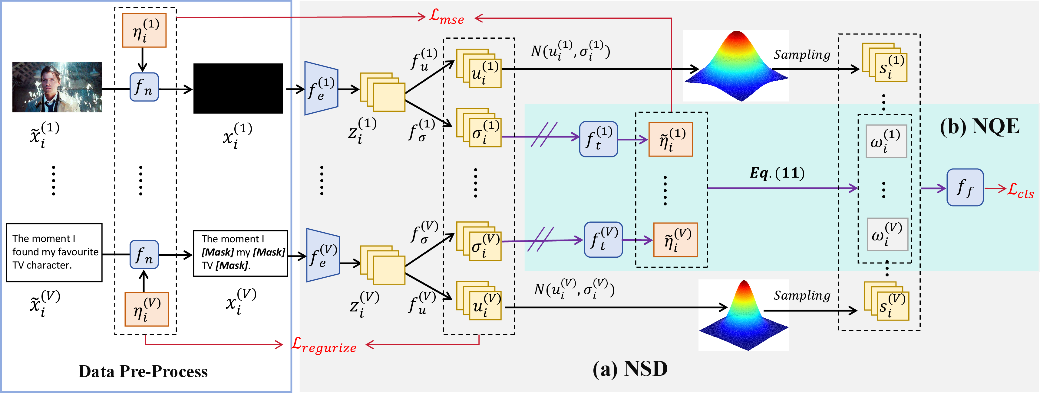
In this work, we propose GIML, a general quality-aware framework for incomplete multimodal learning. It unifies intra-modality and inter-modality missing as continuous modality quality degradation. As illustrated in Fig. 1, GIML consists of two components: a Noise-Semantic Decoupled (NSD) module and a Noise-aware Quality Estimator (NQE). NSD disentangles semantic information from noise-related components at the representation level, preventing noisy features from contaminating task-relevant semantics. This decoupling encourages the model to rely on noise-invariant representations, thereby improving robustness under varying and previously unseen corruption patterns. Meanwhile, NQE formulates modality uncertainty as data degradation and calibrates it via controlled noise injection to learn reliable quality estimates. The estimated quality then modulates fusion weights, ensuring that modality contributions decay smoothly with increasing degradation.
Notations. The main notations used in this work are defined as follows. Let \(\mathcal{D} = \{(X_i, y_i)\}_{i=1}^N\) be a multimodal dataset containing \(N\) samples, where each sample \(X_i = (\tilde{x}_i^{(1)}, \dots, \tilde{x}_i^{(V)})\) consists of \(V\) modality inputs and \(y_i \in \{1, \dots, M\}\) is its label. The \(v\)-th modality encoder is represented by \(f_e^{(v)}\). The noise injection function \(f_n\) applies degradation with intensity \(\eta\) such as Gaussian noise, mask noise, or saltpepper noise to clean modality inputs. The degradation estimator \(f_t^{(v)}\) converts uncertainty into a comparable score for fusion weighting, and \(f_f\) computes the final fused multimodal representation.
3.1 General Incomplete Multimodal Learning↩︎
We first introduce the conventional incomplete multimodal learning, which primarily focuses on inter-modality missing, where certain modalities are entirely absent. Then, we extend it to a more general scenario, where modalities could be partially missing.
Specifically, the multimodal embedding \(\tilde{z}_i^{\tau}\) of \(X_i\) in conventional incomplete multimodal learning can be expressed as follows,
z_i^=f_f(_f,^(1)*_i^(1),...,^(V)*_i^(V))
^(v)=f_e^(v)(_e^v,^v), v
where \({r_i}^{(v)}\) is the embedding of the \(v_{th}\) modality. \(\theta_{f}\) is the parameter for the fusion module. \({\theta_{e}}^{v}\) is the parameters for the \(v_{th}\) modality encoder. \({\delta_i}^{v} \in \{0,1\}\) is the Bernoulli indicator for the \(v_{th}\) modality of \(x_i\). It is randomly set to either 0 or 1 to simulate random modality missing. This makes the model robust for inter-modality missing during inference.
However, in real-world applications, modality inputs are more likely to suffer varying degrees of quality degradation than to be absent, such as impulse-noise contamination or Gaussian blurring. As a result, modality incompleteness often appears in a continuous manner, which cannot be adequately characterized by a binary indicator. To simulate such scenarios, we introduce a noise injection function \(f_n\) that applies degradation with intensity \(\eta_i^{(v)}\) to clean modality inputs: \[{x}_i^{(v)} = f_n(\tilde{x}_i^{(v)}, \eta_i^{(v)}),\]
Here, \(\eta_i^{(v)}\) is a relative calibration signal that controls degradation severity, rather than a physical noise label. \(f_n\) produces various types of corruption based on \(\eta_i^{(v)}\), with larger values indicating heavier degradation, thus spanning from clean to complete absence.
To this end, we extend the conventional binary indicator \({\delta_i}^v \in \{0,1\}\) to a continuous coefficient \(w_i^{(v)} \in [0,1]\) that reflects modality quality. Accordingly, the multimodal embedding of \(x_i\) in general incomplete multimodal learning is formulated as,
z_i^=f_f(_f,z_i^(1)*w_i^(1),...,z_i^(V)*w_i^(V))
z_i^(v)=f_e^(v)(_e^v,x_i^(v)), v
Here, \(w_i^{(v)}=1\) indicates a fully reliable modality, while \(w_i^{(v)}=0\) corresponds to a completely missing modality. Values \(w_i^{(v)} \in (0,1)\) represent partially degraded modalities, where smaller values indicate more severe corruption. In this way, modality degradation can be modeled as a continuous transition from slight corruption to complete absence, enabling a unified formulation of intra-modality degradation and inter-modality missing.
Although GIML enables a unified treatment of modality degradation, it also changes the inference paradigm. Instead of simply checking modality availability, GIML must estimate modality reliability and assign adaptive fusion weights. This introduces two key challenges. First, the model must learn noise-robust representations that generalize across diverse and unseen corruption patterns. Second, it must accurately quantify modality uncertainty and translate it into the weighting coefficient \(w\) for each modality. To address these challenges, we first introduce the Noise-Semantic Decoupled (NSD) module to enhance robustness to diverse noise interference, and then propose the Noise-aware Quality Estimator (NQE) to accurately estimate modality quality for adaptive fusion.
3.2 Noise-Semantic Decoupling↩︎
As discussed above, GIML needs to generalize across diverse and unseen corruption patterns. However, most existing incomplete multimodal learning methods rely on deterministic embeddings, which implicitly entangle task-relevant semantics with degradation patterns. As a result, the learned representation tends to capture corruption-specific characteristics, leading to overfitting and poor generalization to unseen noise conditions. To address this issue, we propose a Noise–Semantic Decoupled (NSD) representation that models modality features as probabilistic distributions rather than deterministic vectors. This design enables an explicit separation between task-relevant semantic information and degradation-induced uncertainty, preventing semantic representations from being contaminated by noise patterns.
For simplicity, we define the probabilistic embedding obeys a multivariate Gaussian distribution. Specifically, given the modality embedding \(z_i^{(v)}\), we parameterize a Gaussian distribution: \[\mu_i^{(v)} = f_\mu^{(v)}(z_i^{(v)}), \quad \log \sigma_i^{(v)} = f_\sigma^{(v)}(z_i^{(v)}).\]
where the mean \(\mu_i^{(v)}\) encodes task-relevant semantic information, while the variance \(\sigma_i^{(v)}\) represents degradation-induced uncertainty.
Now, the representation of each sample becomes a stochastic embedding sampled from \(\mathcal{N}(\mu_i^{(v)}, (\sigma_i^{(v)})^2 \mathbf{I})\). Nevertheless, the sampling operation is not differentiable. Thus, we consider the reparameterization trick [20] to enable backpropagation: \[s_i^{(v)} = \mu_i^{(v)} + \sigma_i^{(v)} \odot \epsilon, \quad \epsilon \sim \mathcal{N}(0,\mathbf{I}).\]
Moreover, to explicitly enforce the separation between semantics and degradation, we introduce two complementary constraints. First, a cross-entropy classification loss \(\mathcal{L}_{cls}^{(v)}\) is applied to the sampled representation \(s_i^{(v)}\), encouraging the mean \(\mu_i^{(v)}\) to preserve discriminative semantic information even under stochastic perturbations. Second, we introduce a degradation-aware prior: \[\mathcal{L}_{reg}^{(v)} = \frac{1}{N} \sum_{i=1}^{N} KL\Big[ \mathcal{N}(\mu_i^{(v)}, (\sigma_i^{(v)})^2 \mathbf{I}) \;\|\; \mathcal{N}(0, (\eta_i^{(v)})^2 \mathbf{I}) \Big].\]
This prior aligns the predicted variance \(\sigma_i^{(v)}\) with the degradation intensity \(\eta_i^{(v)}\), preventing degradation-related variations from being absorbed into the semantic mean. The prior mean is set to zero to avoid imposing additional semantic bias on \(\mu\). Consequently, semantic information and degradation uncertainty are captured in different statistical dimensions, allowing the model to learn noise-invariant semantic representations and improving robustness to diverse and unseen noise conditions.
3.3 Noise-aware Quality Estimator↩︎
The proposed NSD module improves robustness to diverse noise patterns by decoupling semantic information from noise interference. However, effective fusion also requires accurately estimating the severity of modality degradation to assign appropriate weights. However, existing approaches typically measure modality reliability using unsupervised statistics derived from model predictions [25] or feature distributions [26], which often become misaligned with the true degradation level when noise is either too weak or too severe. To address this limitation, we propose a lightweight Noise-aware Quality Estimator (NQE) \(f_t^{(v)}\), which learns to predict the intrinsic noise intensity of each modality through controlled perturbations, enabling accurate and reliable quality estimation across the full degradation spectrum.
Specifically, NQE establishes an explicit mapping from the uncertainty \(\sigma_i^{(v)}\) produced by NSD to the degradation intensity:
\[\hat{\eta}_i^{(v)} = f_t^{(v)}(\sigma_i^{(v)}).\]
Unlike prior methods that rely on implicit reliability inference, NQE is trained with direct supervision using the ground-truth degradation intensity \(\eta_i^{(v)}\): \[\mathcal{L}_{mse}^{(v)} = \frac{1}{N} \sum_{i=1}^{N} \left( \hat{\eta}_i^{(v)} - \eta_i^{(v)} \right)^2.\]
The calibrated degradation estimates \(\hat{\eta}_i^{(v)}\) are then used to guide quality-aware fusion. Following the inverse-variance principle established in ARL [37], we compute adaptive modality weights as
\[\omega_i^{(v)} = \frac{ V \cdot \sum_{u \neq v} (\hat{\eta}_i^{(u)})^2 }{ \sum_{k=1}^{V} (\hat{\eta}_i^{(k)})^2 },\]
Since the degradation scores are explicitly calibrated to the true corruption levels, modalities with higher estimated degradation are adaptively down-weighted, while more reliable modalities contribute more to the fused representation. This explicit calibration facilitates stable fallback to missing-modality modeling.
Finally, the overall training objective of GIML integrates all loss terms: \[\mathcal{L} = \mathcal{L}_{cls}^{f} + \beta_1 \sum_{k=1}^V \mathcal{L}_{cls}^{(k)} + \beta_2 \mathcal{L}_{reg} + \beta_3 \mathcal{L}_{mse}.\] Here, \(\mathcal{L}_{cls}^{f}\) denotes the multimodal task loss computed on the fused representation, and \(\mathcal{L}_{cls}^{(k)}\) represents the unimodal classification loss for the \(k\)-th modality. \(\mathcal{L}_{reg}\) is the regularization term introduced in the NSD module, while \(\mathcal{L}_{mse}\) supervises the noise intensity prediction in the noise-aware quality estimator.
4 Experiment↩︎
4.1 Datasets↩︎
CREMA-D [52] is an audio-visual dataset for emotion recognition, containing 7,442 video clips labeled with six basic emotions. The dataset is split into 6,698 training samples and 744 testing samples.
Kinetics-Sounds (KS) [53] is a subset of the Kinetics dataset focusing on human actions observable both visually and aurally. It consists of 19,000 ten-second video clips spanning 34 action categories, with 15,000 clips for training, 1,900 for validation, and 1,900 for testing.
MVSA-Single [54] is a multimodal sentiment analysis dataset of social media posts, containing paired images and text. Each sample is labeled with a positive, negative, or neutral sentiment. In this work, we follow the train/validation/test split defined in [55] to evaluate cross-modal sentiment recognition.
MOSI [56] is a benchmark dataset for multimodal sentiment analysis, containing audio, visual, and textual modalities. It includes 2,199 video clips extracted from 93 monologue videos, each annotated with a sentiment score ranging from -3 (strongly negative) to 3 (strongly positive). For evaluation, we adopt a binary sentiment setting, considering only positive versus negative labels, to test the model’s ability to handle multimodal information in real-world scenarios.
NVGesture [57] is a large-scale hand gesture dataset with 25 gesture classes performed by 20 participants under varying lighting and background conditions. The dataset contains multiple modalities captured by a Kinect sensor. In our experiments, we follow the official train/validation/test split and use the RGB and Depth modalities for multimodal learning.
| Dataset | |||||||||||||||||
| TMDC | GIML | ||||||||||||||||
| Acc | F1 | Acc | F1 | Acc | F1 | ||||||||||||
| (0.0,0.0) | AV | 67.03 | 67.82 | 73.94 | 74.08 | ||||||||||||
| (0.5,0.5) | 61.64 | 62.67 | 67.80 | 67.78 | |||||||||||||
| (0.1,0.5) | 61.85 | 63.90 | 68.18 | 68.13 | |||||||||||||
| (0.5,0.1) | 66.28 | 67.37 | 72.64 | 72.64 | |||||||||||||
| (0.3,0.7) | 57.35 | 60.04 | 62.93 | 62.80 | |||||||||||||
| (0.7,0.3) | 65.31 | 65.19 | 67.34 | 67.37 | |||||||||||||
| (0.0,-) | A | 52.69 | 54.15 | 55.57 | 55.13 | ||||||||||||
| (0.5,-) | 48.40 | 50.38 | 50.34 | 50.07 | |||||||||||||
| (–,0.0) | V | 44.54 | 48.96 | 60.38 | 60.21 | ||||||||||||
| (–,0.5) | 41.28 | 40.95 | 55.30 | 54.72 | |||||||||||||
| (0.0,0.0) | AV | 60.54 | 62.39 | 69.51 | 69.22 | ||||||||||||
| (0.5,0.5) | 57.90 | 60.11 | 63.54 | 63.06 | |||||||||||||
| (0.1,0.5) | 57.49 | 59.38 | 65.20 | 64.74 | |||||||||||||
| (0.5,0.1) | 60.44 | 62.32 | 66.76 | 66.40 | |||||||||||||
| (0.3,0.7) | 56.68 | 58.79 | 61.68 | 61.26 | |||||||||||||
| (0.7,0.3) | 58.78 | 60.24 | 63.47 | 63.15 | |||||||||||||
| (0.0,-) | A | 38.25 | 41.21 | 45.13 | 44.66 | ||||||||||||
| (0.5,-) | 36.74 | 36.95 | 41.27 | 40.82 | |||||||||||||
| (–,0.0) | V | 44.63 | 43.25 | 55.80 | 55.22 | ||||||||||||
| (–,0.5) | 41.77 | 39.80 | 50.67 | 50.17 | |||||||||||||
0.1pt
4.2 Experimental settings↩︎
Dataset preprocessing. For CREMA-D, a single frame is randomly sampled per video, and audio is loaded at 22,050 Hz. KS uses three frames per video, with audio at 16,000 Hz. MOSI samples five frames uniformly per video, and NVGesture samples 24 frames uniformly from both RGB and Depth streams. All visual frames are resized to 224×224. For visual and audio modalities, we adopt ResNet [58] as the backbone, and for text we use BERT [59] with the first six layers frozen. Training data contains 50% clean samples and 50% samples with random mask rate ranging from 0.0 to 1.0 at intervals of 0.1, simulating diverse real-world inputs.
Missingness setting. In our experiments, we introduce two types of missingness: Mask and Gaussian. Mask sets a proportion of pixels to zero. In extreme cases, this results in a fully black image, simulating complete visual or audio dropout. All performance comparison experiments are conducted with mask noise. Besides, we also introduce Gaussian noise as the unseen noise to study the generalization ability of GIML.
Training. All models are trained using Stochastic Gradient Descent (SGD) with a momentum of 0.9 and a weight decay of 1e-4, with an initial learning rate of 1e-3. Batch sizes are set to 64 for CREMA-D and KS, and 32 for the other datasets. During training, model selection is performed based on the average validation accuracy on both clean samples and those with median noise intensity. Accuracy and weighted F1-score are used as the primary evaluation metrics, denoted as Acc (%) and F1 (%) in the tables, respectively.
4.3 Comparison with State-of-the-art Methods↩︎
2pt
c>p1.2cm |>p0.6cm |>p0.9cm >p0.9cm |>p0.9cm >p0.9cm |>p0.9cm >p0.9cm & & & &
& & Acc & F1 & Acc & F1 & Acc & F1
(0.0, 0.0) & & 77.54 & 76.51 & 76.56 & 75.65 & 77.73 & 77.36
(0.5, 0.5) & & 68.28 & 67.51 & 69.57 & 69.17 & 71.37 & 70.29
(0.1, 0.5) & & 76.17 & 75.46 & 75.39 & 74.67 & 76.68 & 76.00
(0.5, 0.1) & & 68.52 & 67.24 & 69.30 & 67.94 & 70.98 & 70.04
(0.3, 0.7) & & 73.09 & 72.37 & 72.93 & 72.42 & 73.28 & 72.28
(0.7, 0.3) & & 63.12 & 61.57 & 63.09 & 61.96 & 66.02 & 64.71
(0.0, -) & & 77.73 & 76.63 & 75.20 & 74.04 & 78.48 & 78.21
(0.5, -) & & 69.53 & 68.55 & 69.22 & 68.20 & 70.47 & 69.58
(-, 0.0) & & 49.41 & 38.84 & 50.78 & 45.81 & 51.17 & 42.60
(-, 0.5) & & 48.87 & 40.25 & 50.94 & 37.66 & 50.78 & 48.50
2pt
c>p1.6cm |>p0.6cm |>p0.9cm >p0.9cm |>p0.9cm >p0.9cm |>p0.9cm >p0.9cm & & & &
& & Acc & F1 & Acc & F1 & Acc & F1
(0.0, 0.0) & & 48.13 & 49.03 & 46.43 & 47.48 & 56.22 & 55.79
(0.5, 0.5) & & 47.84 & 48.56 & 46.60 & 47.71 & 52.99 & 54.26
(0.1, 0.5) & & 47.76 & 48.73 & 46.76 & 47.53 & 56.51 & 57.37
(0.5, 0.1) & & 48.34 & 49.33 & 47.68 & 48.69 & 55.39 & 55.98
(0.3, 0.7) & & 48.30 & 49.41 & 46.10 & 47.13 & 53.94 & 55.47
(0.7, 0.3) & & 48.09 & 49.14 & 47.10 & 47.98 & 53.78 & 54.53
(0.0, -) & & 40.21 & 40.43 & 38.22 & 38.68 & 52.49 & 52.52
(0.5, -) & & 39.63 & 39.88 & 38.67 & 38.97 & 44.27 & 45.35
(-, 0.0) & & 38.42 & 35.64 & 36.97 & 34.28 & 51.16 & 51.78
(-, 0.5) & & 38.42 & 35.55 & 38.76 & 35.73 & 51.12 & 52.01
2pt
c>p1.8cmc|>p0.6cmc|>p0.9cmc>p0.9cmc|>p0.9cmc>p0.9cmc|>p0.9cmc>p0.9cm & & & &
& & Acc & F1 & Acc & F1 & Acc & F1
(0.0, 0.0, 0.0) & & 79.07 & 79.02 & 71.34 & 71.34 & 80.82 & 80.76
(0.1, 0.3, 0.5) & & 65.36 & 65.46 & 62.54 & 62.62 & 67.55 & 67.55
(0.5, 0.3, 0.1) & & 76.97 & 77.01 & 70.82 & 70.89 & 77.67 & 77.60
(0.0, 0.0, –) & & 53.10 & 53.22 & 51.88 & 51.99 & 54.29 & 54.05
(0.1, 0.5, –) & & 51.04 & 51.15 & 54.55 & 54.63 & 52.83 & 50.61
(0.5, 0.1, –) & & 49.01 & 46.65 & 47.93 & 47.76 & 53.56 & 53.67
(0.0, –, 0.0) & & 79.24 & 79.23 & 76.50 & 76.53 & 81.11 & 81.08
(0.1, –, 0.5) & & 66.94 & 66.95 & 66.01 & 66.08 & 69.88 & 69.95
(0.5, –, 0.1) & & 76.09 & 76.16 & 71.60 & 71.61 & 78.78 & 78.63
(–, 0.0, 0.0) & & 79.30 & 79.25 & 75.92 & 75.82 & 80.85 & 80.80
(–, 0.1, 0.5) & & 66.01 & 66.08 & 62.45 & 62.49 & 68.54 & 68.61
(–, 0.5, 0.1) & & 77.49 & 77.48 & 74.61 & 74.63 & 78.57 & 78.55
(0.1, –, –) & & 52.02 & 49.81 & 54.46 & 54.51 & 55.45 & 55.49
(0.5, –, –) & & 50.27 & 42.80 & 50.54 & 49.70 & 54.11 & 54.19
(–, 0.1, –) & & 51.28 & 51.37 & 51.43 & 51.36 & 52.65 & 52.56
(–, 0.5, –) & & 49.80 & 49.28 & 51.25 & 51.27 & 51.92 & 49.56
(–, –, 0.1) & & 77.11 & 77.15 & 76.79 & 76.83 & 78.45 & 78.41
(–, –, 0.5) & & 66.28 & 66.33 & 66.64 & 66.71 & 68.48 & 68.46
Table 1 reports results on CREMA-D and Kinetics-Sounds under varying intra-modality and inter-modality missing. Across the full degradation spectrum, from fully available modalities to completely missing ones, GIML consistently outperforms TMDC[24] and T2DR [23]. On CREMA-D with fully available modalities \((0.0,0.0)\), GIML achieves 73.94% accuracy compared to 66.99% for TMDC and 67.93% for T2DR. Even under severe intra-modality missing \((0.3,0.7)\), it maintains a clear advantage. A similar trend is observed on Kinetics-Sounds, where GIML consistently achieves the best performance across all settings.
Under imbalanced degradation ratios, such as \((0.1,0.5)\) or \((0.5,0.1)\), GIML consistently performs best. Existing methods do not explicitly account for modality reliability during fusion, allowing low-quality modalities to interfere with decisions. In contrast, GIML estimates modality reliability at the sample level and adjusts fusion weights accordingly, suppressing unreliable modalities while emphasizing informative ones.
To evaluate generalization across different modality combinations and modality numbers, we conduct experiments on MVSA-Single (visual–text, Table ¿tbl:tab:experiments95vt95mask?), NVGesture (RGB–Depth, Table ¿tbl:tab:experiments95rd95mask?), and CMU-MOSI (audio–visual–text, Table ¿tbl:tab:experiments95avt95mask?). These datasets cover both bimodal settings and a three-modality scenario. GIML consistently achieves superior or at least competitive performance across all settings. These results demonstrate that GIML generalizes well across diverse modality combinations and remains effective when scaling from two to multiple modalities, highlighting its modality-agnostic and scalable design for incomplete multimodal learning.
4.4 Robustness to Unseen Noise Intensity↩︎
| Dataset | |||||||||||||||||
| TMDC | GIML | ||||||||||||||||
| Acc | F1 | Acc | F1 | Acc | F1 | ||||||||||||
| (0.0,0.0) | AV | 65.79 | 64.42 | 72.47 | 72.43 | ||||||||||||
| (0.5,0.5) | 61.25 | 61.43 | 66.17 | 66.45 | |||||||||||||
| (0.1,0.5) | 61.98 | 59.80 | 67.80 | 67.70 | |||||||||||||
| (0.5,0.1) | 65.34 | 64.39 | 71.36 | 71.40 | |||||||||||||
| (0.3,0.7) | 58.68 | 58.67 | 65.68 | 65.65 | |||||||||||||
| (0.7,0.3) | 63.68 | 62.55 | 66.66 | 66.66 | |||||||||||||
| (0.0,-) | A | 52.41 | 52.25 | 54.89 | 54.59 | ||||||||||||
| (0.5,-) | 49.80 | 51.26 | 51.53 | 51.68 | |||||||||||||
| (–,0.0) | V | 41.88 | 41.07 | 60.46 | 59.98 | ||||||||||||
| (–,0.5) | 40.04 | 39.16 | 55.65 | 55.40 | |||||||||||||
| (0.0,0.0) | AV | 58.34 | 58.37 | 69.94 | 69.53 | ||||||||||||
| (0.5,0.5) | 57.63 | 57.53 | 63.16 | 62.68 | |||||||||||||
| (0.1,0.5) | 56.86 | 55.89 | 65.31 | 64.86 | |||||||||||||
| (0.5,0.1) | 59.11 | 58.24 | 66.29 | 65.87 | |||||||||||||
| (0.3,0.7) | 56.11 | 53.31 | 61.80 | 61.40 | |||||||||||||
| (0.7,0.3) | 57.79 | 54.85 | 63.55 | 63.35 | |||||||||||||
| (0.0,-) | A | 38.38 | 39.48 | 45.78 | 45.33 | ||||||||||||
| (0.5,-) | 36.82 | 37.00 | 41.27 | 40.84 | |||||||||||||
| (–,0.0) | V | 44.32 | 41.01 | 54.39 | 53.79 | ||||||||||||
| (–,0.5) | 41.29 | 38.46 | 49.64 | 48.93 | |||||||||||||
1pt
To evaluate robustness to unseen noise intensities, the model is trained on a subset of corruption levels and evaluated on previously unseen ones. Specifically, we train the models using mask rates of 0.2, 0.4, and 0.6, and test them on unseen intensities of 0.1, 0.3, 0.5, and 0.7. The results are reported in Table 2 and can be compared with Table 1.
Across both CREMA-D and KS, GIML exhibits only marginal performance degradation on unseen noise levels and consistently maintains superior or competitive performance compared with TMDC and T2DR. In contrast, TMDC and T2DR show noticeable performance drops when evaluated under corruption intensities not observed during training, particularly under severe intra-modality degradation or imbalanced missing ratios. This is because TMDC and T2DR implicitly treat corruption levels as discrete conditions, which restricts their ability to generalize beyond the training noise configurations. In contrast, GIML models modality degradation as a continuous variable \(\hat{\eta}\) and explicitly learns the mapping from degradation severity to modality reliability. As a result, the model can naturally interpolate to unseen noise intensities and dynamically adjust fusion weights according to modality quality, leading to more stable performance across continuous degradation scenarios.
We further examine whether \(\hat{\eta}\) captures relative degradation severity. As reported in Table 4, \(\hat{\eta}\) exhibits strong Spearman correlation with \(\Delta f\), the cosine distance between clean and corrupted features, on mask-trained models under Gaussian corruptions. This confirms that \(\hat{\eta}\) reflects continuous degradation levels, providing a rationale for the model’s robust performance on unseen intensities. This also partially accounts for GIML’s robustness to noise type specificity.
4.5 Generalization to Unseen Noise Types↩︎
3pt
c c|ccc ccc & & &
& & TMDC & T2DR & GIML & TMDC & T2DR & GIML
& (0,0) & 66.99 & 67.93 & 74.18 & 60.40 & 62.73 & 69.88
& (2,2) & 37.85 & 35.75 & 54.08 & 42.62 & 36.07 & 58.30
& (2,5) & 45.83 & 14.11 & 61.82 & 35.47 & 27.21 & 58.06
& (5,2) & 26.91 & 16.40 & 36.36 & 31.50 & 26.39 & 47.30
& (0,–) & 52.66 & 53.92 & 55.57 & 38.67 & 41.21 & 45.13
& (2,–) & 21.48 & 19.76 & 26.36 & 28.05 & 21.69 & 34.89
& (–,0) & 46.80 & 48.95 & 61.82 & 46.43 & 44.90 & 53.92
& (–,2) & 45.56 & 38.31 & 62.36 & 27.50 & 24.61 & 35.66
We evaluate cross-noise generalization by training on Mask corruption and testing on Gaussian noise (Table ¿tbl:tab:experiments95av95guassian?). The Gaussian noise is zero-mean with variances denoted as \(r_a,r_v\).
All methods degrade under this distribution shift, with GIML showing the smallest drop, TMDC moderate, and T2DR the largest. The difference stems from representation handling: T2DR and TMDC extract features directly from corrupted inputs, making semantics sensitive to noise type changes. TMDC partially mitigates this via VIB compression. GIML explicitly disentangles semantic features from degradation and uses modality reliability to guide fusion, preventing noise-induced shifts from affecting semantic representations and ensuring robust performance under unseen noise types.
We further evaluate GIML on realistic-style corruptions including fog, rain, snow, and mixed Mask+Gaussian (M+G). Since existing real-world blur/defocus datasets lack aligned audio-visual emotion labels, we synthesize these corruptions on CREMA-D. Table 3 shows that GIML outperforms TMDC in most settings.
| Fog | Rain | Snow | M+G | |||||||
|---|---|---|---|---|---|---|---|---|---|---|
| 2-4 (lr)5-7 (lr)8-10 (lr)11-11 Intensity | 2 | 5 | 7 | 2 | 5 | 7 | 2 | 5 | 7 | (2,2) |
| TMDC | 65.29 | 57.50 | 53.81 | 64.73 | 59.24 | 55.72 | 67.12 | 64.83 | 58.22 | 26.74 |
| GIML | 71.82 | 62.95 | 57.76 | 70.37 | 62.17 | 57.50 | 73.81 | 69.38 | 56.29 | 52.95 |
4.6 Ablation Study↩︎
\(\beta_1\) Ablation. We evaluate the effect of \(\beta_1\), which balances unimodal classification losses \(\mathcal{L}{cls}^{(v)}\) and fusion loss \(\mathcal{L}{cls}^{f}\). A higher \(\beta_1\) emphasizes unimodal supervision, enhancing disentanglement, while a lower \(\beta_1\) favors the fusion objective. Table ¿tbl:tab:experiments95av95gamma? shows that performance remains stable across a reasonable range of \(\beta_1\), indicating that the disentanglement framework effectively isolates semantic features and maintains robust fusion under noisy conditions.
| Metric | Mask / Gaussian |
|---|---|
| A \(\rho(\hat{\eta}, \Delta f)\) | 0.991 / 0.973 |
| V \(\rho(\hat{\eta}, \Delta f)\) | 0.991 / 0.955 |
| A \(\rho(\mathrm{var}, \Delta f)\) | 0.927 / 0.982 |
| V \(\rho(\mathrm{var}, \Delta f)\) | 1.000 / 0.891 |
3pt
3pt
c>p1.2cmc|>p0.6cmc|>p0.9cmc>p0.9cmc>p0.9cmc>p0.9cm & &
& & 2.0 & 3.0 & 4.0 & 5.0
(0.0,0.0) & & 72.45 & 71.16 & 73.94 & 71.72
(0.5,0.5) & & 65.59 & 65.56 & 67.80 & 66.51
(0.0,–) & & 52.55 & 52.42 & 55.57 & 54.70
(0.5,–) & & 50.24 & 50.19 & 50.24 & 50.89
(–,0.0) & & 60.38 & 61.67 & 60.38 & 61.77
(–,0.5) & & 51.75 & 53.55 & 55.30 & 53.60
Module Ablation. We investigate the contributions of the modality quality estimation (NQE) and semantic disentanglement (NSD) modules.
For GIML-NQE, the learned quality weights are disabled by setting \(w^{(v)}=1\). Table ¿tbl:tab:experiments95av95NQE? reports results under varying modality missing rates. Using uniform weights slightly reduces performance when missing rates are unbalanced, indicating that NQE improves the reliability of modality weighting.
For GIML-NSD, semantic disentanglement is removed by feeding the raw features \(z^{(v)}\) directly into the fusion module instead of the disentangled semantic features \(s^{(v)}\). Table ¿tbl:tab:experiments95av95NSD? shows results under Gaussian noise, where this causes modest reductions in generalization and discriminability, highlighting that NSD facilitates extraction of robust semantic features for multimodal fusion. We further analyze the semantic-uncertainty decoupling of NSD. For semantics, under A/V missing rates of 0.5, we compute “Sep.=Inter./Intra.” on corrupted features, where “Intra.” is the sample-to-class-center distance and “Inter.” is the class-center distance. A larger “Sep.” indicates clearer class structure, and Table 5 shows that \(\mu\) is more class-structured than the raw feature \(z\). For uncertainty, Table 4 shows that variance correlates with \(\Delta f\).
c|cc cc & &
& GIML & GIML-NQE & GIML & GIML-NQE
(0.0,0.0) & 73.94 & 72.66 & 69.51 & 67.45
(0.1,0.5) & 68.18 & 68.15 & 65.20 & 61.96
(0.5,0.1) & 72.64 & 67.69 & 66.76 & 65.29
(0.3,0.7) & 62.93 & 63.68 & 61.68 & 57.73
(0.7,0.3) & 67.34 & 63.39 & 63.47 & 62.40
6pt
c c|cc cc & & &
& & GIML & GIML-NSD & GIML & GIML-NSD
& (0,0) & 74.18 & 73.92 & 69.88 & 68.68
& (2,2) & 54.08 & 48.95 & 58.30 & 52.12
& (2,5) & 61.82 & 45.56 & 58.06 & 39.39
& (5,2) & 36.36 & 23.66 & 47.30 & 44.36
& (0,–) & 55.57 & 54.57 & 45.13 & 45.11
& (2,–) & 26.36 & 18.82 & 45.23 & 35.76
& (–,0) & 61.82 & 62.37 & 53.92 & 55.85
& (–,2) & 62.36 & 45.56 & 35.66 & 36.99
| Modality | \(z\) Sep. | \(\mu\) Sep. |
|---|---|---|
| Audio | 0.70 | 1.51 |
| Visual | 0.66 | 1.88 |
6pt
| Variant | Acc. | \(\rho(\mathrm{var}, \Delta f)\) | \(\rho(\hat{\eta}, \Delta f)\) |
|---|---|---|---|
| Full | 67.41 | 0.927 / 1.000 | 0.991 / 0.991 |
| w/o \(L_{reg}\) | 65.83 | 0.336 / 0.273 | 1.000 / 1.000 |
| w/o \(L_{mse}\) | 64.01 | 1.000 / 1.000 | 0.018 / 0.527 |
Roles of \(L_{reg}\) and \(L_{mse}\). We conduct component ablations under Mask corruption. As shown in Table 6, the full model achieves the best “Acc.”, showing that the two losses are related but not redundant. \(\Delta f\) is the cosine distance between clean and corrupted features. Removing \(L_{mse}\) mainly weakens the \(\hat{\eta}\)-\(\Delta f\) correlation, while removing \(L_{reg}\) mainly weakens the var-\(\Delta f\) correlation. Thus, \(L_{mse}\) calibrates NQE, whereas \(L_{reg}\) regularizes the uncertainty.
5 Conclusion↩︎
This paper introduces General Incomplete Multimodal Learning (GIML), a unified framework for multimodal learning under diverse forms of modality incompleteness. While existing methods mainly focus on inter-modality missing, and a few studies consider intra-modality corruption, they typically treat the two problems separately. In contrast, GIML models modality conditions from mild noise to complete absence as a continuous degradation spectrum, enabling a unified treatment of both intra-modality degradation and inter-modality missing. To support this formulation, we develop a Noise-aware Quality Estimator (NQE) for accurate degradation estimation and a Noise–Semantic Decoupled (NSD) module to improve robustness to diverse and unseen noise patterns. Extensive experiments demonstrate that the proposed framework achieves robust and generalizable multimodal learning across diverse degradation scenarios.
References↩︎
Corresponding author.↩︎