Smart Scissor: Coupling Spatial Redundancy Reduction and CNN Compression for Embedded Hardware
July 08, 2026
Abstract
Scaling down the resolution of input images can greatly reduce the computational overhead of convolutional neural networks (CNNs), which is promising for edge AI. However, as an image usually contains much spatial redundancy, e.g., background pixels, directly shrinking the whole image will lose important features of the foreground object and lead to severe accuracy degradation. In this paper, we propose a dynamic image cropping framework to reduce the spatial redundancy by accurately cropping the foreground object from images. To achieve the instance-aware fine cropping, we introduce a lightweight foreground predictor to efficiently localize and crop the foreground of an image. The finely cropped images can be correctly recognized even at a small resolution. Meanwhile, computational redundancy also exists in CNN architectures. To pursue higher execution efficiency on resource-constrained embedded devices, we also propose a compound shrinking strategy to coordinately compress the three dimensions (depth, width, resolution) of CNNs. Eventually, we seamlessly combine the proposed dynamic image cropping and compound shrinking into a unified compression framework, Smart Scissor, which is expected to significantly reduce the computational overhead of CNNs while still maintaining high accuracy. Experiments on ImageNet-1K demonstrate that our method reduces the computational cost of ResNet50 by 41.5% while improving the top-1 accuracy by 0.3%. Moreover, compared to HRank, the state-of-the-art CNN compression framework, our method achieves 4.1% higher top-1 accuracy at the same computational cost. The codes and data are available at https://github.com/ntuliuteam/smart-scissor
1 Introduction↩︎
Modern convolutional neural networks (CNNs) continue to break previous accuracy records with the advances in large-scale datasets [1]–[4] and network architecture innovation [5]–[8]. Naturally, the accuracy improvement comes at the cost of higher computational overhead [5], [9], [10]. Recently, there is a trend deploying CNNs in edge environments [11] to mitigate the latency and privacy concerns. However, the prohibitive computational cost impedes the deployment of advanced models onto resource-constrained edge devices. To enable edge applications like autopilot to benefit from the development of neural networks, efforts have been made to compress CNNs for a better trade-off between accuracy and model overhead, such that they can be easily deployed onto various edge hardware devices.
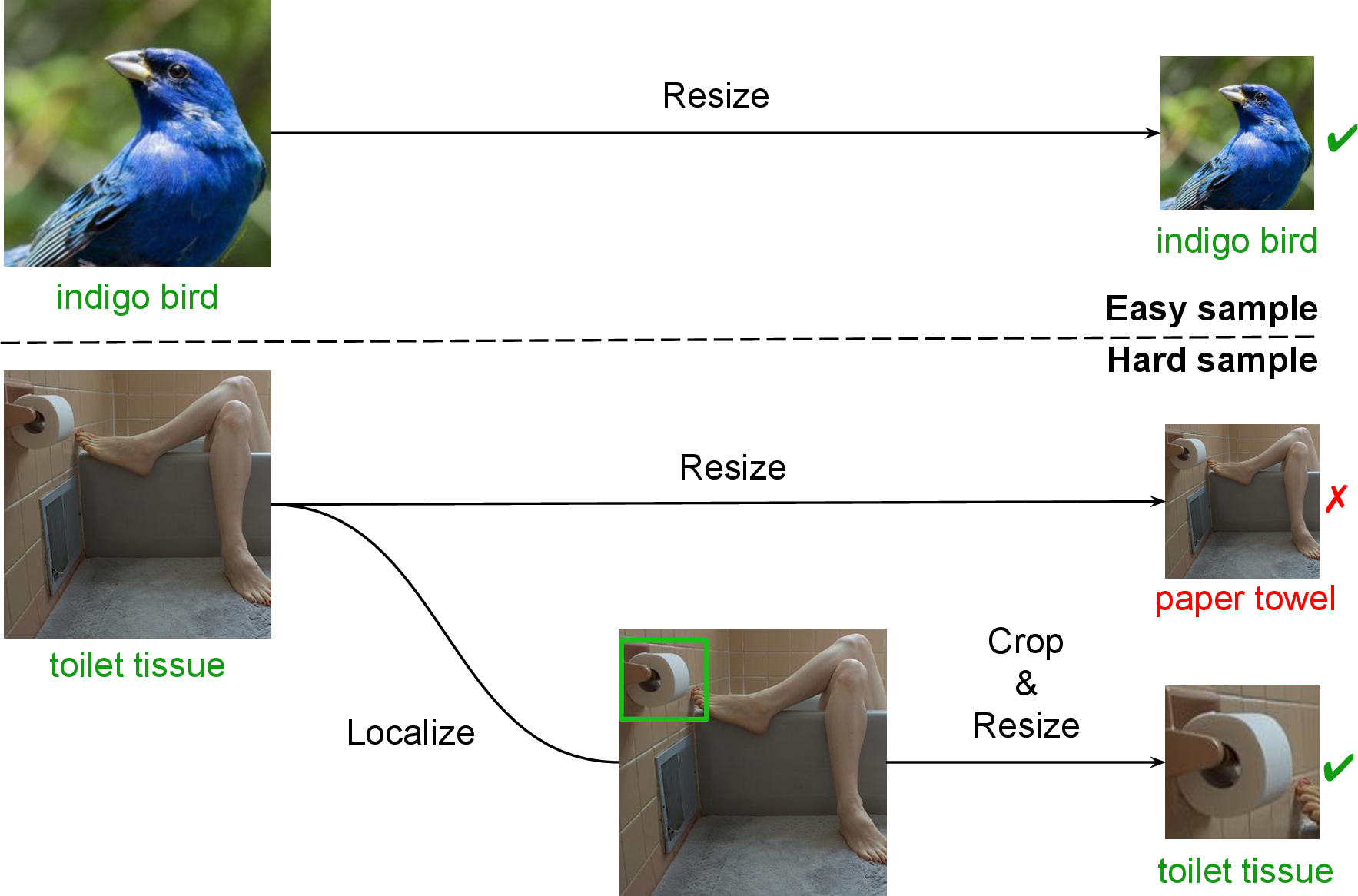
The computational cost, i.e., the Multiply-Accumulate Operations (MACs) of a CNN mainly result from gigantic network architectures and high-resolution input images (e.g., 224\(\times\)224 for ImageNet). To reduce the cost, on the one hand, network architecture pruning [12]–[15] devotes to removing the redundancy in network architectures to construct more compact networks. For instance, MobileNets [16] and Slimmable networks [14] yield ‘thinner’ networks by using less channels in each layer, which reduces the computation and memory footprint. On the other hand, as the MACs of a CNN reduce quadratically with respect to the image resolution, many works resize the input images to a smaller resolution (e.g., 112\(\times\)112) to reduce the computational cost [16]–[18]. However, different images correspond to diverse classification difficulties. As demonstrated in Figure 1, easy samples with clear foreground can be correctly recognized even at a smaller resolution. While for hard samples, as the foreground object only occupies a small portion of the whole image, directly shrinking the image will lose the details of the object, leading to a wrong prediction. In contrast, if we only crop the foreground patch for inference, hard samples can also be correctly classified at a small resolution. However, existing image preprocessing methods, e.g., ResizedCenterCrop (RCC), crop all images in a static manner and cannot achieve such instance-aware fine cropping, which motivates our work.
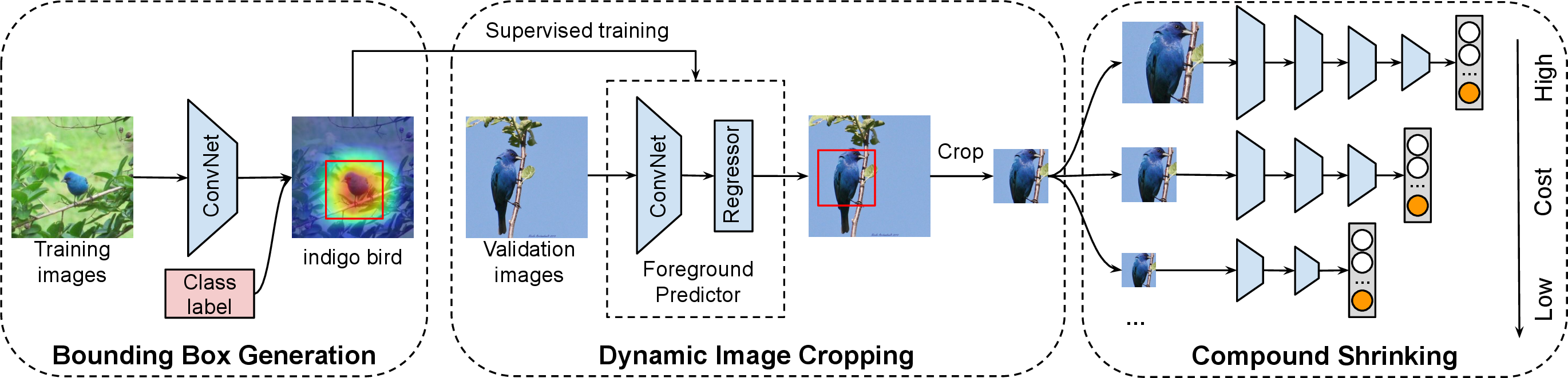
In this paper, we propose a dynamic image cropping (DIC) framework to facilitate the inference with low-resolution images, thereby reducing the costs of CNNs and boosting the deployment of CNNs onto resource-constrained edge devices. DIC first efficiently localizes the most discriminative foreground of the input image with a lightweight foreground predictor, then the detected foreground region will be preserved and the redundant background will be discarded. By this means, DIC is capable of generating fine-cropped images with less spatial redundancy, thereby improving the inference accuracy even under low-resolution settings. To train the foreground predictor on large-scale classification datasets, we first employ a visualization technique, Grad-CAM [19], to generate the salience map of each training image to indicate the most discriminative foreground. Based on the salience map, we then automatically generate a bounding box annotation for each training image. Subsequently, we use the image-box pairs to train the predictor in a supervised manner. Once the foreground predictor is trained, it can be directly applied to any CNN backbones without modification.
Meanwhile, to deal with the redundancy in network architectures for higher execution efficiency, we propose a compound shrinking (CS) strategy to jointly compress the three dimensions (depth, width, resolution) of a CNN. We first investigate the impact of shrinking each dimension on accuracy. Based on that, we then calculate the optimal shrinking coefficient for each dimension to coordinate the shrinking of different dimensions to achieve the highest compression rate while still maintaining the accuracy. Eventually, DIC and CS are seamlessly combined to form a deep compression framework, Smart Scissor, where an image is firstly cropped by DIC, then the cropped patch will be resized to the resolution calculated by CS and sent to the model compressed by CS for efficient inference. With our approach, both the spatial redundancy in images and the architecture redundancy in networks are reduced and thus the execution of CNNs on embedded hardware is accelerated.
The main contributions of this paper are summarized as follows:
We propose a dynamic image cropping framework to reduce the spatial redundancy in images. We introduce a lightweight foreground predictor to efficiently localize the foreground object and conduct instance-aware dynamic cropping. With the finely cropped images, CNNs can yield accurate predictions using a smaller resolution, which greatly reduces the computational cost of CNNs.
We also propose a compound shrinking strategy to coordinately shrink the three dimensions (depth, width, resolution) of a CNN. We first quantify the impact of each dimension on accuracy, and then compute the optimal shrinking coefficient for each dimension accordingly. By this means, we can greatly reduce the redundancy in network architectures while still maintaining high accuracy.
We seamlessly combine the dynamic image cropping and compound shrinking into a deep compression framework, which is able to optimally adapt the model cost to meet different resource constraints of embedded hardware.
Experiments on ImageNet-1K demonstrate that our method reduces the MACs of ResNet50 by 41.5% while improving the top-1 accuracy by 0.3%. In addition, our method achieves 4.2% higher top-1 accuracy with similar MACs and 54.3% less parameters compared to the most widely used image cropping method, ResizedCenterCrop (RCC). In low MACs regime, our approach also outperforms HRank [12] by a remarkable improvement (4.1%) in top-1 accuracy.
2 Related Work↩︎
Smart Scissor is mainly related to object discovery and neural network compression, so we discuss the related works in this section. Object discovery: Object discovery algorithms have made impressive progress. Among them supervised object detection (SOD) [20]–[23] achieves relatively high accuracy on well annotated datasets, such as COCO [2] and Pascal VOC [24]. However, the difficulties in building larger detection datasets hinder the further development of SOD. Weakly supervised object discovery (WSOD) [19], [25]–[27] is able to coarsely localize objects of interest with only image-level labels, which makes WSOD applicable to more large-scale datasets without bounding box annotations, such as ImageNet [1]. Class activation map (CAM) [27] is able to visualize the importance of different regions of the input image by utilizing the output of the pooling layer at the end of CNNs. Grad-CAM [19] further generalizes CAM by using the gradients to calculate the importance of different pixels, which makes it applicable to more CNN architectures. ACoL [28] designs a CNN architecture with two branches to adversarially learn the full region of objects. CutMix [29] randomly blends different regions of images to improve the localization accuracy. However, the huge computational cost and latency make both the SOD (e.g., SSD) and WSOD inapplicable in our context, i.e., resource-constrained embedded hardware.
CNN compression: To compress CNNs for better on-device performance, different approaches have been proposed to remove the redundancy of CNNs. Deep Compression [30] removes neurons from kernels, which achieves a high compression rate. However, the obtained sparse networks need special hardware to accelerate. [12], [14], [16], [31] build compact CNNs by removing channels from each layer, which can speed up the execution of CNNs on off-the-shelf hardware. Among them MobileNetV2 [16] and Slimmable networks [14] uniformly reduce the channels in all layers. Instead, HRank [12] and Taylor pruning [31] prune the channels in a layer-wise manner. Besides compressing the network architecture, some works focus on reducing the spatial redundancy in images. MobileNetV2 [16] and MnasNet [17] use smaller resolutions to improve the performance on mobile devices. DR-ResNet [18] proposes a dynamic resolution network to reduce the computational cost. GFNet [32] employs reinforcement learning to select multiple small patches instead of using the whole image to accelerate CNNs. However, these methods only consider reducing the redundancy in a single dimension and thus only achieve a limited compression rate. In contrast, jointly compressing all dimensions promises a better trade-off between the compression rate and accuracy.
3 The Smart Scissor Framework↩︎
In this section, we first outline the design of Smart Scissor and then describe each submodule in detail.
As demonstrated in Figure 2, given a classification dataset \(\mathcal{D}\) and a classification network \(\mathcal{N}\). We first exploit Grad-CAM to generate the salience map of all training images in \(\mathcal{D}\), and then we generate a bounding box for each image according to the salience map and form a bounding box label set \(\mathcal{B}\). Thereafter, we utilize the image-box pairs {\(\mathcal{D}_i\), \(\mathcal{B}_i\)} to train a lightweight predictor. Meanwhile, for a given MACs budget \(\mathcal{M}\), we use CS to quickly calculate the desired resolution and shrink the network accordingly. During inference, an image will be first fed into the predictor to quickly output the boundary of the foreground object, then the detected object is cropped. Finally, the cropped patch is resized to the calculated resolution and sent to the compressed network \(\mathcal{N}_s\) for fast inference.
3.1 Bounding Box Generation↩︎
As aforementioned, dynamically cropping the foreground for inference is promising in reducing computation and improving accuracy. However, for classification datasets like ImageNet, there is no out-of-the-box position annotation for the foreground object. Moreover, the position of the foreground object varies in different images, which makes it difficult to efficiently localize the foreground object.
To address this limitation, we first use Grad-CAM [19] to automatically generate the position annotations. Specifically, let the class label of the given image be \(c\). We first perform forward inference with a well-trained CNN (e.g. ResNet50) to obtain the prediction score \(p^c\) for class \(c\), and then conduct backpropagation to compute the gradient of the score \(p^c\) with respect to each activation of the last convolutional layer. Thereafter, the gradients are aggregated within each channel via global average pooling. The obtained scalar for each channel can be seen as the weight of the channel, which can be calculated as follows: \[a_k^c = \overbrace{\frac{1}{Z}\sum_i\sum_j}^{\textit{pooling}} \overbrace{\frac{\partial p^c}{A_{ij}^k}}^{\textit{gradients}}\] where \(a_k^c\) is the weight of channel \(k\) for class \(c\), and \(A_{ij}^k\) is a single activation indexed by \(i\) and \(j\) in the 2-D feature map of channel \(k\). With the weights of all channels determined, the salience map for class \(c\) can be obtained by computing the weighted sum of all feature maps over the channel dimension, which is formulated as: \[L_{Grad\_CAM}^c = ReLU\underbrace{(\sum_k a_k^c A^k)}_{\textit{linear combination}}\] where \(A^k\) is the 2-D feature map of channel \(k\), and ReLU is used to eliminate the impact of negative activations. Finally, the obtained salience map is upsampled to the same size as the input image via bi-linear interpolation algorithm.
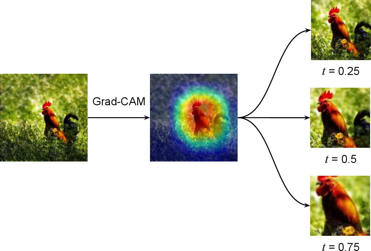
With the salience map generated, we then introduce a simple yet effective strategy to determine the bounding box of the foreground object. Initially, we set the box as the boundary of the image. Subsequently, we shrink the four sides of the box simultaneously, and once a side reaches our preset salience threshold \(t\), the side is frozen. The bounding box is determined after all sides are frozen. Note that it is crucial to appropriately select the value of \(t\) for the final result. As demonstrated in Figure 3, a too small threshold will result in residual background redundancy, while a too large threshold will lose some object features. Therefore, we conduct empirical experiments to determine the optimal threshold value. As shown in Table 1, we achieve the highest accuracy when the threshold \(t\) is set to 0.5. Therefore, we set \(t=0.5\) in the following experiments. Note that more fine-grained searching for \(t\) may further improve the accuracy, but it also increases the search cost. Finally, the generated box annotations are saved in the form of [\(X_{min}\), \(Y_{min}\), \(X_{max}\), \(Y_{max}\)], which denotes the position of the foreground in the image.
| Model | \(\#\)Params | \(\#\)MACs | t | Acc@1 |
|---|---|---|---|---|
| ResNet50 | 25.6 M | 4.1 B | 0 (Baseline) | 76.02 \(\%\) |
| 0.25 | 76.45 \(\%\) | |||
| 0.5 | 76.88 \(\%\) | |||
| 0.75 | 76.32 \(\%\) |
3.2 Dynamic Image Cropping↩︎
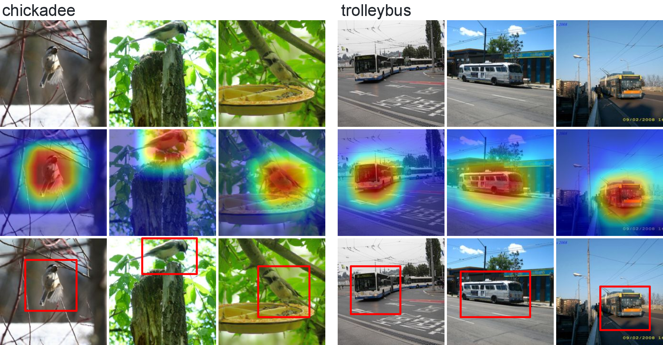
Figure 4 shows that we are capable of accurately localizing the foreground of images with Grad-CAM. However, Grad-CAM cannot be directly applied to edge applications because of the time-consuming backpropagation process. Moreover, Grad-CAM requires the class label as weak supervision, which is unavailable for validation images. To address these issues, we design a foreground predictor to efficiently localize the foreground of input images.
3.2.1 Predictor Architecture↩︎
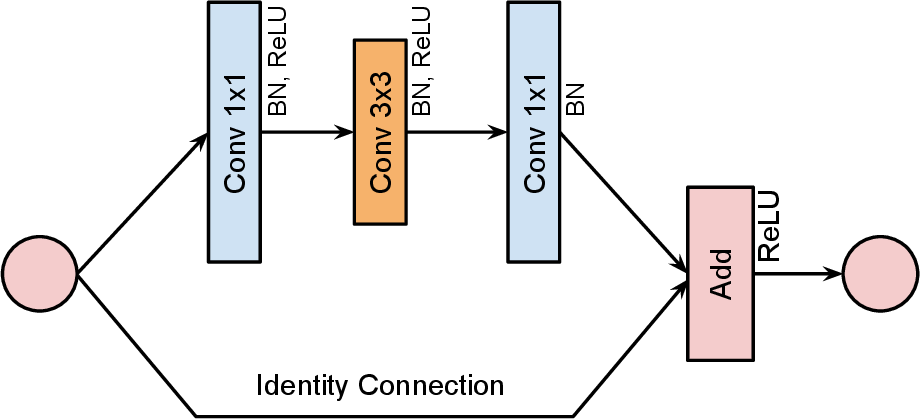
Although dozens of object detectors have been proposed to detect objects from images, such as SSD [21] and Faster R-CNN [22], these detector architectures are completely inapplicable to our task. Particularly, to accurately detect multiple objects from a single image, existing detectors are usually equipped with a heavy feature extractor and a complex region proposal network (RPN), which are extremely time-consuming and unnecessary for image classification where each image only contains one object. Therefore, we discard the design of traditional detectors. Instead, we design the foreground predictor as a lightweight plain CNN, whose detailed architecture is summarized in Table 2. It consists of several residual bottleneck blocks [33] and a fully connected layer as the single-box regressor. As shown in Figure 5, a residual bottleneck contains two convolutional layers with 1\(\times\)1 kernels and one convolutional layer with 3\(\times\)3 kernels in the middle. The computational cost mainly results from the 3\(\times\)3 convolutional layer. Therefore, to reduce the cost and accelerate the predictor, we only stack two residual bottleneck blocks in each stage and each block is only equipped with a small number of channels. Consequently, the proposed predictor only contains 0.27M parameters and 0.09B MACs, which is negligible compared to popular object detectors (e.g., Faster R-CNN with 134.7M (499\(\times\)) parameters and 15.1B (167.8\(\times\)) MACs [34]). Moreover, the small overhead of the foreground predictor can be complemented by the CS module.
3.2.2 Training of Foreground Predictor↩︎
We train the predictor in a supervised manner. First, we generate a bounding box label set \(\mathcal{B}\) for all training images as described in Subsection 3.1, then the labels are utilized to train the predictor. We use the mean square error (MSE) as the loss function. Let \(\mathcal{P}_i=\) [\(X_{min}^p\), \(Y_{min}^p\), \(X_{max}^p\), \(Y_{max}^p\)] be the output of the predictor, and \(\mathcal{B}_i=\) [\(X_{min}^g\), \(Y_{min}^g\), \(X_{max}^g\), \(Y_{max}^g\)] be the generated box label, the loss function can be formulated as: \[\begin{align} \mathcal{L}_{box} = & \;MSELoss(\mathcal{P}_i, \;\mathcal{B}_i) \\ = & \;\frac{1}{4} ((X_{min}^g-X_{min}^p)^2+(Y_{min}^g-Y_{min}^p)^2 \\ & +(X_{max}^g-X_{max}^p)^2+(Y_{max}^g-Y_{max}^p)^2) \end{align}\]
To balance the training overhead and prediction accuracy, we train the predictor with Adam [35] optimizer for 40 epochs. The initial learning rate is set to 1e-3, and the learning rate is scheduled using exponential decay [36]. The training of the box predictor is decoupled with backbone networks. Once the predictor is trained, it can be directly applied to different classification backbones without any training overhead. During inference, the trained predictor will quickly localize the foreground object of the input image and generate a finely cropped image, which significantly reduces the redundancy in the input image.
3.3 Compound Shrinking↩︎
The proposed DIC significantly reduces the redundancy in images, improving the computational efficiency. We observe that redundancy also exists in network architectures (e.g., redundant parameters), and only removing the redundancy in images loses the opportunity to further compress the model for embedded hardware. Besides, [5] demonstrates that jointly adjusting different dimensions promises higher accuracy. To this end, we propose a compound shrinking (CS) strategy to jointly compress the three dimensions (depth, width, resolution) of CNNs to reduce the redundancy in images as well as networks while maintaining the accuracy.
| Stage | Block | Resolution | #C | #L |
|---|---|---|---|---|
| 1 | Conv 3\(\times\)3 | 224 \(\times\) 224 | 16 | 1 |
| 2 | Residual Bottleneck | 112 \(\times\) 112 | 16 | 2 |
| 3 | Residual Bottleneck | 56 \(\times\) 56 | 32 | 2 |
| 4 | Residual Bottleneck | 28 \(\times\) 28 | 32 | 2 |
| 5 | Residual Bottleneck | 14 \(\times\) 14 | 64 | 2 |
| 6 | Pooling & Linear | 7 \(\times\) 7 | 4 | 1 |
| #Params: 0.27M | ||||
| #MACs: 0.09B | ||||
Intuitively, shrinking different dimensions has different impacts on accuracy and model overhead. The core of our compound shrinking strategy is to calculate a shrinking coefficient for each dimension according to their trade-off between accuracy and model overhead. A larger coefficient denotes more radical shrinking. More specifically, the dimension with a steep accuracy drop during shrinking will be assigned a small shrinking coefficient to prevent severe accuracy degradation. To calculate the shrinking coefficients, we first quantify the trade-off of each dimension between accuracy and model overhead. Here we use MACs as the metric to measure the cost of models, because all three dimensions are related to the MACs of a model while only the depth and width can affect the model parameters. Given a MACs budget \(\mathcal{M}\), we first obtain the accuracy drops resulting from separately shrinking different dimensions, which can be represented as: \[\label{eq:acc} \Delta A_s(\mathcal{M}) = A_0 - A_s(\mathcal{M})\tag{1}\] where \(s\in\{d, w, r\}\) represents the shrunk dimension, \(A_s(\mathcal{M})\) denotes the accuracy of the shrunk model, and \(A_0\) denotes the accuracy of the original model. To comply with the rule that the steeper the drop in accuracy, the smaller the coefficient of the corresponding dimension, we design the following equation to determine the shrinking coefficient for each dimension: \[\label{eq:coeff} \mathcal{C}_s(\mathcal{M}) = \frac{\sqrt[3]{\Delta A_d(\mathcal{M}) \cdot \Delta A_w(\mathcal{M}) \cdot \Delta A_r(\mathcal{M})}}{\Delta A_s(\mathcal{M})}\tag{2}\] where \(\mathcal{C}_s(\mathcal{M})\) denotes the shrinking coefficient of the dimension \(s\) (\(s\in\{d, w, r\}\)). Through Equation 1 and Equation 2 , we are able to efficiently calculate the coefficients once we obtain the accuracy degradation of the three dimensions in the given MACs regime.
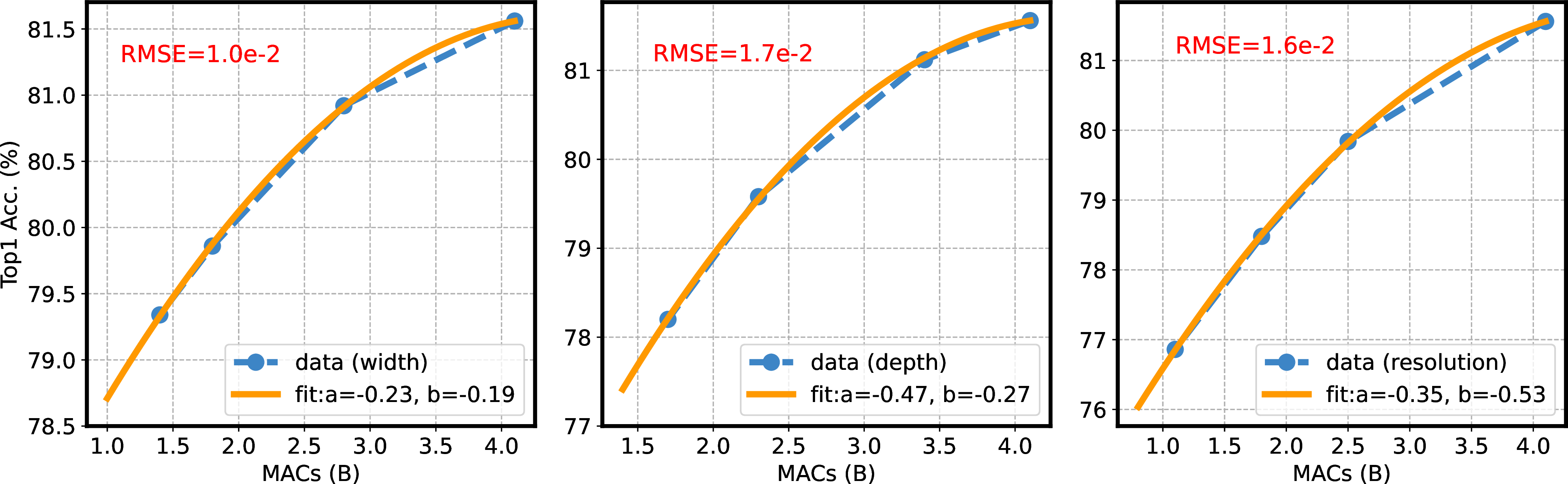
However, the training cost of the compressed models to calculate the accuracy drop is still non-negligible. To mitigate the training overhead, we propose a dimension-wise accuracy estimator to quickly estimate the accuracy of the compressed models and calculate the accuracy degradation resulting from shrinking different dimensions in the given MACs regime. First, we sample a couple of models with different MACs by separately shrinking the three dimensions. As demonstrated in Figure 6, the accuracy distribution of the three dimensions along MACs can be well fitted by a quadratic polynomial. Therefore, we design a simple yet effective polynomial estimator to predict the accuracy with respect to the target MACs \(\mathcal{M}\). The estimator can be formulated as follows: \[A_s(\mathcal{M}) = a_s (\mathcal{M} - \mathcal{M}_0)^2 + b_s (\mathcal{M} - \mathcal{M}_0) + A_0\] where \(\mathcal{M}_0\) is the MACs of the original model. \(a_s\) and \(b_s\) are the hyperparameters to fit for dimension \(s\) (\(s\in\{d, w, r\}\)). Subsequently, we train the dimension-wise estimator using least square regression with the aforementioned sampled data. Figure 6 shows that the proposed estimator can well fit existing data. Due to the simple and intuitive design of the estimator, we only need to sample and train very few models to train the estimator, and this cost is a one-time cost. With the accuracy estimator established, we are capable of directly calculating the accuracy drop and subsequently the shrinking coefficient of each dimension across a wide range of MACs regimes. Consequently, the cost of assigning the coefficients is significantly reduced compared to directly training models to obtain the coefficients.
4 Experimental Results↩︎
In this section, we conduct experiments to comprehensively evaluate Smart Scissor. We compare Smart Scissor with many state-of-the-art (SOTA) methods in terms of accuracy, MACs, on-device latency, and throughput. In addition, we also do ablation experiments to validate the efficacy of each component in our framework.
4.1 Hardware Devices↩︎
The on-device latency and throughput are two important metrics to evaluate the efficiency of CNNs. To demonstrate the on-device performance of our method, we select two representative embedded GPU platforms, NVIDIA AGX Xavier and NVIDIA Jeton Nano, and Intel i7-9750H@2.6GHz CPU to deploy the proposed framework and measure the latency and throughput. The hardware specifications are listed in Table 3.
| Device | Power | Memory/Cache | Performance |
|---|---|---|---|
| AGX Xavier | 15 W | 32 GB | 11 TOPS |
| Jetson Nano | 5 W | 4 GB | 0.47 TFLOPS |
| i7-9750H | 45 W | 12 MB | 0.4 TOPS |
4.2 Datasets↩︎
We evaluate our method on two large-scale datasets, ImageNet-1K [1] and ImageNet-100. ImageNet-1K (a.k.a. ILSVRC 2012) is the most widely exploited dataset for image classification tasks, which consists of 1,000 classes, and each class contains about 1,000 high-resolution (224\(\times\)224) images for training and 50 images for validation. ImageNet-100 is a subset of ImageNet-1K, which is composed by 100 randomly selected classes from ImageNet-1K. The detailed categories of ImageNet-100 is provided in the code repository. All images are preprocessed following a simple configuration as [16], [37].
4.3 Networks↩︎
We implement the Smart Scissor framework with two popular CNN models, ResNet50 [33] and RegNet-X [37] as the baseline backbone networks. For each model, we apply Smart Scissor to reduce the model overhead by removing both the spatial redundancy of images and the architecture redundancy of networks. Moreover, we also report the results of other SOTA model compression approaches on the two models for comparison.
4.4 Optimization Settings↩︎
We use a stochastic gradient descent (SGD) optimizer with a momentum of 0.9 to train the classification networks. On both ImageNet-100 and Imagenet-1K, models are first trained with a batch size of 1,024 for 100 epochs without dynamic image cropping, where the first 5 epochs are for warmup. At this stage, the initial learning rate is set to 2.0 and decayed by exponential learning rate policy with a decay factor of 0.02. Then, we use the proposed dynamic image cropping to fine-tune the pretrained models for 20 epochs with a constant learning rate of 5e-4. To prevent over-fitting, we also use label smoothing with \(\epsilon=0.1\).
4.5 Results on ImageNet-100↩︎
We conduct experiments on ImageNet-100 with both ResNet50 and RegNet-X. In practise, to better demonstrate the improvement of each component, we implement two versions of Smart Scissor, Smart Scissor with only the DIC module (SS-DIC) and Smart Scissor with both the DIC and the CS module (SS-DIC-CS). As a comparison, we use the most popular image cropping method, ResizedCenterCrop (RCC) to crop and resize images. Finally, all models are deployed to the hardware platforms to evaluate the latency and throughput.

| Method | #Params | #MACs | \(\downarrow\) MACs | Acc@1 |
|---|---|---|---|---|
| -Baseline | 23.7 M | 4.1 B | 0.0\(\%\) | 81.6\(\%\) |
| 24.0 M | 4.2 B | -2.4\(\%\) | 82.5\(\%\) | |
| 17.3 M | 3.0 B | 26.8\(\%\) | 82.7\(\%\) | |
| 23.7 M | 3.0 B | 26.8\(\%\) | 80.1\(\%\) | |
| 24.0 M | 2.6 B | 36.6\(\%\) | 80.8\(\%\) | |
| 14.5 M | 2.4 B | 41.5\(\%\) | 81.5\(\%\) | |
| 23.7 M | 1.1 B | 73.2\(\%\) | 76.9\(\%\) | |
| 24.0 M | 1.2 B | 70.7\(\%\) | 77.9\(\%\) | |
| 7.8 M | 1.0 B | 75.6\(\%\) | 79.3\(\%\) |
ResNet50: As shown in Table 4, SS-DIC-CS outperforms the competitors on all metrics. Specifically, compared to the baseline ResNet50 (RCC-Baseline), SS-DIC improves the accuracy by 0.9% with a negligible increase in model parameters (1.2%) and MACs (2.4%), while SS-DIC-CS further pushes up the accuracy improvement to 1.1% with a parameter reduction of 27% and a MACs reduction of 26.8%. In the low complexity regime, SS-DIC-CS achieves 2.4% higher accuracy than RCC with only 33% model parameters (7.8 M v.s. 23.7 M) and less MACs. Meanwhile, Figure 7 indicates that both SS-DIC and SS-DIC-CS outperform RCC by a large margin across a wide spectrum in terms of latency and throughput. Particularly, SS-DIC-CS achieves 79.4% top-1 accuracy with a latency of 4.3 ms on Xavier, which is 0.9% higher in accuracy and 18.9% lower in latency compared to RCC(78.5% top1 accuracy, 5.3 ms). At the same time, the throughput of SS-DIC-CS on Xavier is 232.5 imgs/sec, which is 22% higher than RCC(190.5 imgs/sec). On Nano and Intel i7-9750H CPU, SS-DIC-CS also improves the throughput by 20.6% and 10.1%, and reduces the latency by 17% and 9.1%, respectively.

| Method | #Params | #MACs | \(\downarrow\) MACs | Acc@1 |
|---|---|---|---|---|
| -Baseline | 8.4 M | 1.6 B | 0.0% | 84.8% |
| 8.7 M | 1.3 B | 18.8% | 85.0% | |
| 6.3 M | 1.3 B | 18.8% | 86.1% | |
| 8.4 M | 0.7 B | 56.3% | 82.3% | |
| 8.7 M | 0.8 B | 50.0% | 83.8% | |
| 3.6 M | 0.6 B | 62.5% | 84.0% | |
| 8.4 M | 0.4 B | 75.0% | 80.0% | |
| 8.7 M | 0.5 B | 68.8% | 81.4% | |
| 2.5 M | 0.4 B | 75.0% | 82.8% |
RegNet-X: The experimental results of RegNet-X are summarized in Table 5, where we also observe a significant improvement of our method. SS-DIC-CS outperforms the baseline RegNet-X (RCC-Baseline) with an improvement of 1.3% in accuracy and a reduction of 18.8% in MACs. Meanwhile, SS-DIC-CS reduces the model parameters by 25% (6.3 M v.s. 8.4 M). In the low MACs regime, SS-DIC-CS observes a remarkable 2.8% improvement in accuracy with only 30% parameters (2.5 M v.s. 8.4 M) compared to RCC. As for the real performance on hardware, SS-DIC-CS obtains an accuracy of 84% with 3.6 ms latency on Xavier, which is 0.3% higher in accuracy and 30.8% lower in latency than RCC(83.7% top-1 accuracy, 5.2 ms). Similarly, the latency reductions on Nano and Intel CPU are 31% and 34.6%, respectively. Besides, SS-DIC-CS observes a 44.9% throughput improvement (51.6 imgs/sec v.s. 35.6 imgs/sec) on Nano and a 52.5% throughput improvement (30.2 imgs/sec v.s. 19.8 imgs/sec) on Intel CPU compared to RCC.

4.6 Results on ImageNet-1K↩︎
We evaluate our approach on ImageNet-1K, and compare the evaluation results with many SOTA CNN compression frameworks. In addition, we also compare our compressed models with many popular backbone architectures in different computation regimes.
Comparison with SOTA compression methods: Starting with the baseline ResNet50 model, we implement different model shrinking methods, including RCC, width shrinking (WidthShrink) [16], [38], depth shrinking (DepthShrink) [33], SS-DIC, and SS-DIC-CS, to compress the three dimensions of the model to different MACs regimes and compare their performance. In addition, we also report the performance of multiple SOTA model compression techniques from the related papers, including DR-ResNet50 [18], SSS-ResNet50 [39], Versatile-ResNet50 [40], PFP-A-ResNet50 [41], C-SGD70-ResNet50 [42], GAL-1 [43], HRank [12], and RANet [44]. The comparison results are summarized in Figure 9, which shows that our method achieves the highest accuracy across a wide range of MACs. Particularly, compared to the baseline ResNet50, our method achieves 1.2% accuracy improvement (76.0% to 77.2%) with a negligible increase in MACs (4.1 B to 4.2 B). As we continue to reduce the MACs budget, SS-DIC-CS reduces the MACs by 41.5% (4.1 B to 2.4 B) while still achieving 0.3% higher accuracy (76.0% to 76.3%). In the low MACs regime, SS-DIC-CS remarkably improves the accuracy by 4.2% (70.0% to 74.2%) compared to RCC with similar MACs. In comparison with other SOTA compression methods, our method also achieves the best trade-off between MACs and accuracy. For example, SS-DIC-CS achieves 3.3% higher accuracy (73.2% v.s. 69.9%) than GAL-1 [43] with 37.5% less MACs (1.0B v.s. 1.6B).

Comparison with popular backbones: In this experiment, we apply Smart Scissor to ResNet50 and compare it with other models from the ResNet family, such as ResNet101 and ResNet34, etc. In addition, we also conduct extensive comparison with other popular backbones like DenseNets [45] and the Inception family [46], [47]. As demonstrated in Table 6, in the highest MACs regime, SS-DIC only uses 53.2% of the MACs (4.2 B v.s. 7.9 B) of DenseNet161 to achieve the same level of accuracy, while in the lowest MACs regime, SS-DIC-CS obtains the highest top-1 accuracy (75.6%), which is 5.8% and 2.1% higher than ResNet18 (69.8%) and BN-Inception (73.5%), respectively. The comparison results with other backbones reveal that our method can achieve promising results without redesigning the network architecture, which avoids the extremely time-consuming exploration of the architecture design space.
| Model | #Params | #MACs | \(\downarrow\) MACs | Acc@1 |
|---|---|---|---|---|
| ResNet50[33] | 25.6 M | 4.1 B | 0.0\(\%\) | 76.0% |
| ResNet101[33] | 44.6 M | 7.9 B | -92.7\(\%\) | 77.4% |
| DenseNet161[45] | 28.7 M | 7.9 B | -92.7\(\%\) | 77.1% |
| InceptionV3[46] | 27.2 M | 5.8 B | -41.5\(\%\) | 77.3% |
| 25.9 M | 4.2 B | -2.4\(\%\) | 77.2% | |
| ResNet34[33] | 21.8 M | 3.7 B | 9.8\(\%\) | 73.3% |
| DenseNet169[45] | 14.2 M | 3.4 B | 17.1\(\%\) | 75.6% |
| 25.9 M | 3.1 B | 24.4\(\%\) | 76.3% | |
| 15.4 M | 2.4 B | 41.5\(\%\) | 76.3 \(\%\) | |
| ResNet18[33] | 11.7 M | 1.8 B | 56.1\(\%\) | 69.8% |
| DenseNet121[45] | 8.0 M | 2.9 B | 29.3\(\%\) | 74.6% |
| BN-Inception[47] | 11.2 M | 2.1 B | 48.8\(\%\) | 73.5% |
| 25.9 M | 1.9 B | 53.7\(\%\) | 74.9% | |
| 13.5 M | 1.8 B | 56.1\(\%\) | 75.6% |
| Method | #Params | #MACs | Latency | Acc@1 |
|---|---|---|---|---|
| ResNet50 | 25.6 M | 4.1 B | 10.6 ms | 76.0% |
| 25.6 M | 1.1 B | 3.0 ms | 70.0% | |
| RandomCrop | 25.6 M | 1.1 B | 2.9 ms | 69.1% |
| 25.9 M | 1.2 B | 3.8 ms | 73.1% | |
| ResShrink | 25.6 M | 1.1 B | 3.0 ms | 70.0% |
| WidthShrink | 8.9 M | 1.2 B | 5.2 ms | 71.2% |
| DepthShrink | 11.1 M | 1.7 B | 5.0 ms | 69.6% |
| 11.4 M | 1.1 B | 4.6 ms | 71.5% | |
| 11.7 M | 1.3 B | 5.5 ms | 74.2% |
4.7 Visualization↩︎
We visualize the bounding boxes generated from both Grad-CAM and our predictor in Figure 10. We can see that the foreground of the most of images only occupies part of the whole images, thus performing inference on the whole image is unnecessary and inefficient, which coincides with our motivation. Moreover, Figure 10 validates that, even though the foreground predictor only contains very limited computation and parameters for higher execution efficiency, it can also accurately localize the main object. With the accurate and quick prediction of the foreground, we are able to remove the background redundancy in images, thereby accelerating the execution of CNNs on resource-constrained edge devices.
4.8 Ablation Study↩︎
To validate the efficacy of both the DIC module and the CS module, we perform comprehensive ablation experiments on ImageNet-1K. First, we only keep the DIC module to separately evaluate its efficacy. The results in Table 7 show that SS-DIC outperforms RCC and RandomCrop remarkably. Specifically, SS-DIC improves the top-1 accuracy by 3.1% compared to RCC with a similar model cost. Subsequently, we evaluate the CS component by comparing it with single-dimension shrinking methods. The results also demonstrate the efficacy of the CS component. Finally, we combine the two modules into the completed framework SS-DIC-CS. Because of the novel design of DIC and CS, we significantly improve the accuracy with a slightly higher latency on Xavier, optimizing the trade-off between accuracy and latency. The ablation experiments reveal that both DIC and CS contribute to the final performance.
5 Conclusion↩︎
In this paper, we propose a deep compression framework, Smart Scissor, to comprehensively reduce the redundancy in both input images and network architectures, thereby facilitating the efficient inference on edge devices. First, we rethink the image cropping strategy for CNNs, and we find that existing static cropping methods introduce much redundancy in images. To reduce the redundancy in images, we propose a dynamic image cropping framework. The proposed framework first employs a foreground predictor with negligible overhead to quickly localize the important foreground region, and only the detected foreground will be utilized for inference, which remarkably reduces the computational cost. Meanwhile, to remove the redundancy in network architectures, we also propose a compound shrinking strategy, which coordinately shrinks the three dimensions of CNNs according to their importance to the final accuracy. By this means, the compound shrinking strategy is expected to comprehensively compress CNNs. Finally, the dynamic image cropping and compound shrinking are integrated to work coordinately for the optimal trade-off between accuracy and costs. Extensive and comprehensive experiments demonstrate the efficacy and efficiency of our approach.
6 Acknowledgement↩︎
This study is partially supported under the RIE2020 Industry Alignment Fund – Industry Collaboration Projects (IAF-ICP) Funding Initiative, as well as cash and in-kind contribution from the industry partner, HP Inc., through the HP-NTU Digital Manufacturing Corporate Lab (I1801E0028). This work is also partially supported by Nanyang Technological University, Singapore, under its NAP (M4082282).