1

1 Introduction & Related Work↩︎

Speech-to-text alignment assigns each transcribed word a start and end time in the audio. It is classically produced by finding the best path through a Gaussian-mixture hidden Markov model (GM-HMM) which is still the most accurate aligner for read speech [1]–[5]. Current models, however, differ in what alignment they provide on their own [6]: connectionist temporal classification (CTC) [4], [7] and transducer models [8] have one by construction, whereas attention-based encoder-decoders (AED) [9]–[11] and speech large language models (LLMs) [12]–[14] do not, and their word timings are usually read off the attention weights instead. All of these signals live on the 20 to 80 ms encoder frame grid, which bounds their temporal precision. For AED, reading the timing off the cross-attention is established practice: Whisper emits coarse segment-level timestamp tokens [15], word-level timestamps follow from a dynamic time warping (DTW) of the decoder cross-attention [16] that fine-tuning can sharpen [17], and the alignment-bearing heads can even be selected by an unsupervised heuristic and refined with character-level teacher forcing without any training [18]. Speech LLM self-attention carries a similar alignment, used to constrain text-to-speech synthesis [19] and as a policy for simultaneous translation [20]; forced alignment has separately been cast as a trained LLM task [21].

We study a generic gradient-based alignment that applies to any differentiable speech recognition model. For each transcript token we take the gradient of its teacher-forced log probability with respect to the input, reduce it to a per-frame saliency [22], and decode the resulting token-by-frame matrix into word boundaries with a single dynamic-programming pass (1). As it uses the gradient w.r.t. the input signal, it aligns on the input grid rather than on the coarser encoder grid, and it can correct temporal shifts of the encoder: the encoder is often so powerful that it can displace the signal in time (e.g. with streaming models) or even reverse the time dimension [23]¹, which degrades the native forced alignment, while the gradient should still give a meaningful alignment. It needs no training and no model modification and it applies to all model families. Unlike the attention-based alignment, which first has to find which attention head carries the alignment (hand-picked for Whisper, and unpublished for the other models, so that we have to select it on a labeled development set), the gradient uses one canonical signal, the saliency of the token’s own log probability. In prior work, the same method has been applied to speech recognition AED models [18], [23] and machine-translation models [24].

This work is not a proposal of gradient alignment as the best aligner. A strong native aligner is usually still somewhat better, and the gradient is considerably more expensive. We rather provide a broad and fair analysis of what the gradient alignment is, how well it works across all the model families, and where it wins and loses. Our contributions are:

• We show that the gradient-based alignment applies to all ASR model families: CTC (prefix scores), transducers (RNN-T and TDT, also via prefix scores), AED, and speech LLMs.

• Improved alignment path scoring, where the best alignment path is found via dynamic programming. The cross-attention dynamic time warping (DTW) used by Whisper and CrisperWhisper is a special case of it. Our version improves on that DTW both on the attention and on the gradient signal.

• For the speech LLMs, we read the alignment off their self-attention, the analog of the encoder-decoder cross-attention.

• A comprehensive and fair comparison of sixteen models across the four families, on read (TIMIT) and spontaneous (Buckeye) speech, each against its own native or attention-based alignment, including the tokenization granularity, the input-grid resolution, the recognition-mode alignment, and the compute cost.

• Public source code to reproduce all results including the whole pipeline.

2 Alignments via Gradients↩︎

We can calculate the gradient of the log probability \(p(a_s \mid a_1^{s-1}, x_1^{T'})\) of some target label \(a_s \in \mathcal{A}\) (the label vocabulary) in label position \(s\), given the input \(x_1^{T'}\) and the history \(a_1^{s-1} \in \mathcal{A}^{s-1}\) of previous labels, w.r.t. an input frame \(x_t\). The transcript \(a_1^S\) has \(S\) labels and the input \(T'\) frames; the saliency matrix and the alignment below have \(T\) time frames: \(T = T'\) when the gradient is taken at the input, or the number of encoder frames when it is taken at an encoder layer. Comparing the norm of these gradients over the time frames \(t\) will give us an indication of the importance of each frame for this specific output label \(a_s\). Specifically, we calculate the log norm² \[G_{s,t} := \log \left\Vert \nabla_{x_t} \log p(a_s \mid a_1^{s-1}, x_1^{T'}) \right\Vert_p \in \mathbb{R}. \label{eq:grad}\tag{1}\] The matrix \(\log \operatorname{softmax}_{T} G\) in 1 shows the alignment clearly.

Note that \(\log p(a_s \mid a_1^{s-1}, x_1^{T'})\) is straightforward to compute for an AED model or speech LLM (we exclude the EOS label here), and was done in a similar way in [18], [23]. It is possible for CTC and transducer as well, using the prefix scores [25] which can be calculated efficiently using dynamic programming.

To use this to get some alignment, we need to define which alignment label topology we allow (mapping \(a_1^S\) to \(y_1^T\)) and how to score one particular alignment \(y_1^T\) such that we can search for the one with the highest score.

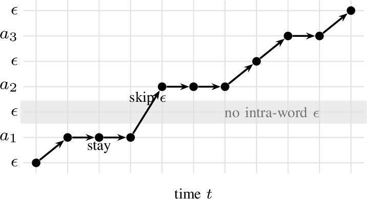
For the label topology, we map \(a_1^S\) to \(y_1^T\) over \(\mathcal{Y} = \mathcal{A} \cup \{\epsilon\}\), letting each real label repeat over consecutive frames with \(\epsilon\) (blank/silence) labels in between. We write this as a finite state automaton with enumerated states \(Y_1^{2S+1} = (\epsilon, 1, \epsilon, 2, \dots, S, \epsilon)\), whose \(S+1\) blank states sit before the first label, between adjacent labels, and after the last. A topology is fixed by which of these blank states it permits, the rest being disallowed. Our default is a word-level topology: a blank only at word boundaries (before the first word, after the last, and between adjacent words), forbidding blanks inside a word, as we evaluate word boundaries. The full, CTC-like topology instead permits every blank (unlike CTC, we do not force a \(\epsilon\) between two equal labels \(a_s = a_{s+1}\)), and a variant with no interior silence keeps only the leading and trailing blank, so adjacent tokens follow each other directly. We decode all topologies with the standard time-synchronous Viterbi search (as in CTC), advancing one frame per step, so every token spans at least one frame. Whisper and CrisperWhisper instead align the cross-attention by DTW, which additionally allows vertical transitions (advancing the token within a frame), so adjacent tokens may overlap by up to one frame; with no interior silence and without the log of 3 , our decoder reduces to that DTW up to those vertical transitions (¿tbl:tab:alignopts-dtw?). We search for an allowed state sequence \(r_1^T\), \(r_t \in \{1,\dots,2S+1\}\), compatible with \(a_1^S\), that maximizes \[\operatorname{GradScore}(r_1^T) = \sum_{t=1}^T \begin{cases} G'_{Y_{r_t},t}, & Y_{r_t} \ne \epsilon, \\ \beta_t, & Y_{r_t} = \epsilon, \end{cases} \label{eq:grad-score}\tag{2}\] with a token score \(G'\) and a silence score \(\beta_t\) defined below. The best \(r_1^T\) is found via dynamic programming (2), and the alignment \(y_1^T\) read off with \(y_t = a_{Y_{r_t}}\) for non-blank states and \(y_t = \epsilon\) otherwise.

The token score is the over-time log-softmax of the (optionally energy-weighted) saliency, \[G'_{s,t} = \log\operatorname{softmax}_{T} (G + \rho \log E)_{s,t} , \label{eq:grad-token-score}\tag{3}\] where \(\rho \ge 0\) is a weighting (\(\rho = 0.5\) by default; \(\rho = 0\) disables it) and \(E_t \in [0,1]\) a smoothed audio-energy envelope on the frame grid: from the waveform \(x\) we form the windowed root-mean-square energy \(\tilde{E} = \sqrt{w * x^2}\), with \(w\) a normalized \(25\) ms Hann window (\(\sum_i w_i = 1\)) and \(*\) convolution, sample it at the frame centers \(c_t\), and normalize by its maximum, \(E_t = \tilde{E}_{c_t} / \max_{t'} \tilde{E}_{c_{t'}}\). The energy weight suppresses the gradient’s spurious response in silent frames.

The silence score \(\beta_t\) admits the constant blank of CTC, but also a self-calibrating blank derived from the per-frame statistics of the token scores. Let \(\mu_t\) and \(\sigma_t\) be the mean and standard deviation of \(\{G'_{s,t}\}_s\) over the labels \(s\) (taken at \(\rho = 0\), so the blank calibrates against the raw saliency). We consider \[\beta_t = \begin{cases} \gamma, & \text{(constant)} \\ \mu_t + \kappa\,\sigma_t, & \text{(z-score)} \\ \mu_t - \lambda\,z(E_t)\,\sigma_t, & \text{(energy)} \end{cases} \label{eq:silence-score}\tag{4}\] with \(z(E_t) = (E_t - \bar{E})/\operatorname{std}(E)\) the z-score of the energy over the \(T\) frames (\(\bar{E}\) and \(\operatorname{std}(E)\) its mean and standard deviation), and hyperparameters \(\gamma\) (constant level), \(\kappa\) and \(\lambda\). The energy blank is a VAD-style silence emission: in a low-energy frame \(z(E_t) < 0\) raises \(\beta_t\) above the token mean, so the frame goes to the blank; in speech frames \(\beta_t\) drops below the token scores.

max width=

max width=

max width=

max width=

max width=

max width=

max width=

max width=

max width=

max width=

max width=

max width=

3 Experimental Setup↩︎

We evaluate sixteen models from the four families. For reference we run two dedicated aligners, a GM-HMM via MFA [3], and MMS-FA [26], [27], a wav2vec 2.0 [28] CTC model built specifically for forced alignment. For CTC we further use XLS-R on phonemes [29], [30], Parakeet CTC [31], OWSM-CTC [32], [33], and a streaming FastConformer-CTC [34]. For the transducers we use Parakeet RNN-T [31] and TDT [35], and the streaming FastConformer-RNN-T [34] and Emformer [36], [37]. The AED models are Whisper base and large-v3 [15], CrisperWhisper [17], and OWLS-1B [38], and the speech LLMs are Voxtral [39], Phi-4-multimodal (Phi-4-MM) [40], and Canary-Qwen [41]. We align on TIMIT (test) [42] and on Buckeye spontaneous speech [43], both with gold word boundaries. For Buckeye we use a \(5\) h subset stratified by speaker (all speakers represented proportionally), split at every \(\geq 1\) s inter-word silence, then split any piece still longer than \(18\) s at its largest internal gap³. We report the word-boundary error (WBE), i.e. the mean per-word start and end absolute error, averaged over all words in the corpus⁴, and the accuracy at a collar, i.e. the fraction of all boundaries within \(50\) ms over the corpus. We compare each model against its own alignment, i.e. the CTC or transducer forced alignment on the model’s own emission (the “posteriors”), the AED cross-attention DTW [16], and, for the speech LLMs, the analogous text-to-audio self-attention, decoded by the same dynamic program as the gradient scores. We select the attention heads by per-head WBE on TIMIT development gold and average the top 8 heads. In hypothesis mode, where the recognition differs from the reference, we match the words by identity and report an identity-gated F1 at a \(50\) ms collar together with the matched WBE.

4 Results↩︎

4.0.0.1 Alignment quality across model families

¿tbl:tab:per-model-methods? compares the gradient alignment versus each model’s own native or attention aligner, across CTC, AED, transducer and speech-LLM families. Gradient alignment is competitive on every family, beats the native alignment where it is weak (the streaming models, Canary-Qwen), and at the starred best encoder depth it also beats the Whisper-large-v3 cross-attention. The streaming posteriors’ large error is largely a systematic emission-delay bias rather than scatter (¿tbl:tab:boundary-offsets? 1); the same table shows that gradient alignment shifts both boundaries together (a positional lead) rather than shrinking the word like the posteriors do.

¿tbl:tab:hyp? aligns each model’s own recognition (identity-gated F1 at a \(50\) ms collar and matched WBE), showing that gradient alignment remains usable when the hypothesis differs from the reference.

4.0.0.2 Tokenization and the attention baseline

¿tbl:tab:char-vs-subword-family? justifies the tokenization we use throughout: the gradient alignment uses character targets for the AED and speech-LLM families and subword targets for CTC and transducers, while every attention or posterior baseline uses the model’s native subword tokens. Character targets improve the gradient markedly for the autoregressive families (on Whisper-large-v3 and Voxtral the char gradient is well below the subword gradient), but they do not help the model-native attention aligners, and for the non-autoregressive CTC and transducer, which have no per-character acoustic emission, char-level collapses: char targets are consistently worse than subword for both the gradient and the posteriors, in the worst cases by an order of magnitude.

4.0.0.3 Ablations

The grad. score per-token reduction (¿tbl:tab:gradscore?) moves WBE by only a few ms across the \(p\)-norms, while the plain sum is clearly worse, and gradient versus gradient-\(\times\)-input [44], [45] is within \(\sim\)​1–3 ms with neither winning consistently. Multi-pass attribution (SmoothGrad [46], VarGrad [47], Integrated [48] and Expected Gradients [49]) does not beat the single-pass gradient (numbers omitted here). Most decoding options behave consistently (¿tbl:tab:alignopts-silence? ¿tbl:tab:alignopts-energy? ¿tbl:tab:alignopts-dtw?): the gradient is active even in silence and needs the energy-aware (\(\lambda\approx 2\)) or z-score blank, whereas the attention is already silence-aware and a constant blank suffices; the z-score blank is the energy-free option that matches the energy one for gradients. The audio-energy token-weighting exponent matters little around our default and behaves consistently across the blank schemes (¿tbl:tab:alignopts-energy?). For the cross-attention DTW, the dominant gain over the original Whisper heuristic is the gold-tuned head selection (its curated set includes some near-useless heads); the Whisper-DTW setting is exactly our decoder with the log-compression and the blank state removed, and energy weighting helps the gradient but not the cross-attention DTW.

4.0.0.4 Where the gradient is taken

For MMS-FA, which is a wav2vec 2.0 model [28] (¿tbl:tab:wav2vec-resolution?), the gradient localizes best at the feature-projection output (20 ms encoder grid); finer levels (the convolutional feature encoder, or the raw waveform pooled down to sample resolution) do not help, and the raw-waveform gradient is noisier. ¿tbl:tab:encoder-depth? sweeps the depth for Whisper-large-v3 and the FastConformer-CTC, from the log-mel input through the encoder to its output (the activation just before the decoder / CTC linear): the sharpest gradient is at an intermediate depth (three quarters of the Whisper encoder, the L24 of the starred row in ¿tbl:tab:per-model-methods?; a quarter for the FastConformer-CTC), not the input, and in the streaming FastConformer-CTC the encoder’s time shift accumulates with depth, so its output gradient ends as delayed as its posteriors (1).

4.0.0.5 Speech-LLM prompt influence

Gradient alignment is robust to the prompt used across all the speech LLMs and across the gradient-vs-self-attention signal (numbers omitted).

4.0.0.6 Inter-CTC

OWSM-CTC has intermediate CTC losses [32], [33], which we can use to take the gradient at each block of the encoder (¿tbl:tab:owsm-per-layer?). Interestingly, the earlier blocks are better than the later ones, both for the gradient and for the native CTC alignment.

4.0.0.7 Time stretch

Under audio time-stretch (numbers omitted), the same upsampling mechanism acts with opposite sign: it hurts a fine-grid model (MMS-FA) but helps a coarse-grid one (Voxtral) at mild factors.

4.0.0.8 Compute cost

The only extra cost over the native methods is the per-token backward (¿tbl:tab:cost?); the forward and the DP decode are shared, and for the CTC the per-token prefix-score lattice backward dominates.

5 Conclusion↩︎

Gradient alignment produces a usable word alignment for every model and family we tried, including the speech LLMs that have no built-in word aligner. It is usually a little behind a strong native aligner, but clearly better where that alignment is weak, as on the streaming models and Canary-Qwen, and on Whisper-large-v3 it even beats its cross-attention at the best encoder depth. Our decoder also improves on Whisper’s cross-attention DTW itself (¿tbl:tab:alignopts-dtw?). Its input-grid resolution lets finer character targets improve accuracy, which the coarse attention grid cannot exploit. The per-token backward makes it much more expensive than a single forward, so we do not propose it as a practical aligner. The result is rather that one training-free input saliency aligns every differentiable ASR model across all four families, in some cases even better than the model’s own alignment. Beyond alignment, the gradient also serves as an analysis tool.

0

Acknowledgment↩︎

This work was partially supported by NeuroSys, which as part of the initiative “Clusters4Future” is funded by the Federal Ministry of Research, Technology and Space BMFTR (funding IDs 03ZU2106DA and 03ZU2106DD), and by the project RESCALE within the program AI Lighthouse Projects for the Environment, Climate, Nature and Resources funded by the Federal Ministry for the Environment, Nature Conservation, Nuclear Safety and Consumer Protection (BMUV), funding ID: 67KI32006A. The authors gratefully acknowledge the computing time provided to them at the NHR Center NHR4CES at RWTH Aachen University (project number p0023999). This is funded by the Federal Ministry of Education and Research, and the state governments participating on the basis of the resolutions of the GWK for national high performance computing at universities (www.nhr-verein.de/unsere-partner).

AI-Generated Content Disclosure↩︎

We used AI assistants (large language models) substantially in this work, to help set up and run the experiments, to debug and write parts of the code, and to draft and edit parts of this paper. All results were verified by the authors, who take full responsibility for the content.

References↩︎