G-PROBE: Cross-FOV Place Recognition and
Certainty-Coupled Localization for 3D Point Clouds
July 07, 2026
Abstract
Global localization from 3D point clouds remains challenging under limited or asymmetric fields of view (FOV), which fail to provide the dense, symmetric coverage that place recognition methods assume. We present G-PROBE, a learning-free global localization framework that removes this assumption. A virtual sensor decomposition runs the same pipeline, by design, on configurations ranging from a narrow-FOV sensor to a panoramic or multi-sensor rig. The front-end enumerates cross-FOV branch ensembles that encode heading hypotheses for heading-invariant place recognition. A score-scale-invariant, tuning-free \(\gamma\)-SGRT suppresses heading aliasing under partial FOV and provably becomes inert at symmetric \(360^\circ\). The back-end, CG-GICP, refines a coarse full-cloud GICP with a pass restricted to high-certainty co-observed points selected by a bird’s-eye-view certainty map (a by-product of front-end scoring). This certainty coupling links descriptor evaluation to 6-DoF metric pose estimation without an external verification module. Evaluated on five LiDAR datasets and three modalities (mechanical, solid-state, FMCW), G-PROBE attains the highest learning-free multi-session F1 on average and is competitive in panoramic single-session settings. Where hand-crafted and zero-shot supervised baselines collapse under wide\(\leftrightarrow\)narrow cross-sensor pairing, it remains usable end-to-end (up to \(55.0\%\) vs.\({\le}6.8\%\) success), and under FOV asymmetry (\(360^\circ\!\to\!60^\circ\)) it retains \({\sim}54\%\) Recall@1, \({\sim}18\times\) the strongest learning-free baseline.
3D Point Clouds, LiDAR, Global Localization, Certainty-Guided Registration, Cross-FOV Heading Invariance, Place Recognition
1 Introduction↩︎
Global localization, the estimation of a robot’s metric pose directly from a prior map without an initial pose estimate, is fundamental to robust autonomous navigation and loop closure in SLAM. Place recognition is well established for cameras [1] and dense \(360^\circ\) LiDAR [2], [3], but the mature LiDAR solutions implicitly assume a dense, symmetric, panoramic field of view (FOV). Localization on diverse, FOV-constrained point clouds has received comparatively little attention, even as the sensors that produce them are increasingly deployed for their long sensing range and compact, mechanically robust solid-state design. A recent survey likewise names limited FOV, cross-sensor configuration, and unbalanced matching among the open problems of global LiDAR localization [4].
1.1 The Heterogeneity and Cross-FOV Heading Problem↩︎
The central challenge addressed in this paper is the mismatch between the panoramic assumptions of existing methods and the constrained, heterogeneous FOVs of modern sensor configurations.
Problem 1: Sensor Heterogeneity and Modality Invariance. Emerging autonomous systems deploy a mix of spinning, directional solid-state, and frequency-modulated continuous-wave (FMCW) LiDARs, each with distinct point densities, noise distributions, and FOVs. Modality-invariant matching across these sensor types remains an open challenge. Recent methods attempt this using overlap-based deep learning (HeLiOS [5], following the overlap supervision of OverlapNet [6]) or Vision Foundation Models (VFMs) [7], but require supervised training to adapt to new sensors and, absent that adaptation, degrade on unseen scanning patterns (§6.4).
Problem 2: Heading-Dependent Coverage. Many platforms observe only a partial azimuth: a single narrow-FOV solid-state LiDAR (e.g., a \(70^\circ\) Livox) or multiple sensors with a combined blind spot. A robot revisiting from a different heading then observes the scene through a different angular sector, so polar descriptors that gain rotation invariance by full-ring column shifting [2] become unreliable. A narrow FOV also admits only a small angular slice of the scene at once, leaving little distinctive structure for reliable matching and compounding the geometric degeneracy of long featureless paths that corrupts both recognition and registration.
1.2 Limitations of Existing Approaches↩︎
Prior works address these problems only in isolation (§2): panoramic descriptors assume dense \(360^\circ\) coverage [2], [3], FOV-aware methods rely on fixed heuristics or supervised fine-tuning [7], [8], and degeneracy-aware registration and odometry reason purely in geometric space [9], [10]. None of them links the per-region reliability the descriptor computes to the alignment the registration performs. Hand-crafted descriptors discard their internal state after retrieval, and registration ignores observational confidence.
1.3 Probing Reliability from Geometry↩︎
Rather than learn modality invariance, we probe per-bin structural reliability directly from sensor geometry. During cross-FOV ensemble evaluation the descriptor computes per-bin mutual occupancy agreement between query and database. Bins on solid structure show high mutual occupancy and low uncertainty, FOV-boundary and sparse bins the opposite. This single computation serves both stages of the pipeline. The mutual-agreement score drives the cross-FOV match, addressing the heterogeneity and heading problems above. The same internal state, extracted as a bird’s-eye-view (BEV) certainty map \(c(r,s)\in[0,1]\) and fed to registration, yields a certainty-coupled architecture in which the front-end informs the back-end about observational reliability. The coupling thus incurs no additional cost.
1.4 Contributions↩︎
This paper makes three contributions:
Cross-FOV Ensemble Place Recognition (§4): A framework that decomposes any sensor configuration (a gap-free multi-sensor rig or a single sensor; Definition 1) into cross-FOV branch descriptors with FOV-overlap weighting, parameterized solely by the total azimuthal coverage and its orientation rather than the physical sensor count, enabling heading-invariant retrieval without panoramic FOV assumptions. A score-scale-invariant Softmax Gap Ratio Test (\(\gamma\)-SGRT) adds tuning-free, FOV-adaptive suppression of heading aliasing, yielding a uniqueness probability (\(P_{dom}\)) that flags heading-ambiguous matches.
Certainty-Guided Registration (CG-GICP) (§5): A two-pass coarse-to-fine Generalized-ICP in which a per-bin BEV certainty map, a by-product of G-PROBE’s occupancy scoring, selects the high-certainty co-observed points for the refinement pass. This recognition-to-registration coupling operates without any external verification module (e.g., RANSAC) and suppresses the worst-case error tail from one-sided, FOV-boundary correspondences, leaving the typical case unchanged (§6.6).
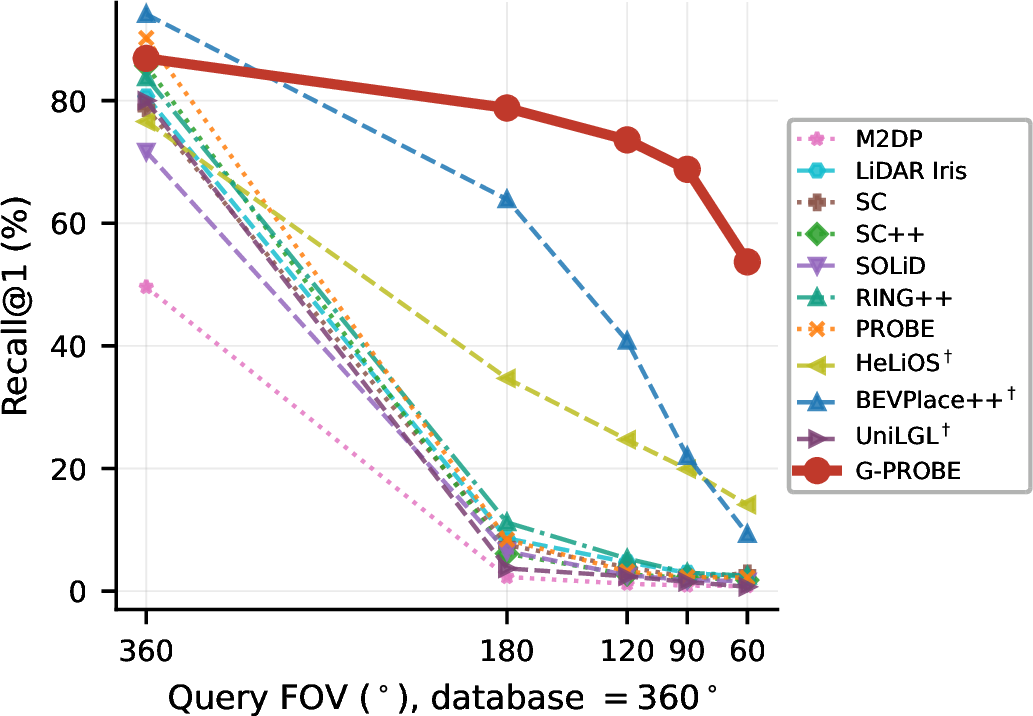
Heterogeneous Evaluation (§6): An evaluation of the learning-free, CPU-only system across five datasets and three LiDAR modalities (mechanical, solid-state, FMCW), with FOV co-visibility ground truth, via a \(3{\times}3\) cross-sensor place recognition matrix, cross-day end-to-end metric localization, an FOV-controlled cross-sensor study, and a registration ablation. G-PROBE attains the highest learning-free multi-session F1 on average and the best cross-FOV robustness among all baselines under FOV asymmetry. Under extreme asymmetry (\(360^\circ\!\to\!60^\circ\)) it retains \({\sim}54\%\) Recall@1, \({\sim}18\times\) the strongest learning-free baseline, while most prior descriptors collapse below 4% (Fig. 1).
Relation to PROBE. This paper builds on PROBE [11], a symmetric-FOV, retrieval-only descriptor that introduced the closed-form analytical marginalization over continuous translations (§[sec:scoring]). PROBE was validated predominantly in the panoramic, full-ring setting. Under FOV restriction its retrieval keys degrade, with only a brute-force, retrieval-bypassing variant recovering partial accuracy on KITTI, and it explicitly flagged this missing-sector key distortion as an open problem. G-PROBE inherits this probabilistic core and extends it from a single descriptor to a complete global localization system: (i) the panoramic, full-ring retrieval becomes a general cross-FOV framework (virtual sensor decomposition, FOV-overlap masking, \(\gamma\)-SGRT) whose per-pair occupancy divergence reduces exactly to PROBE’s under homogeneous full co-visibility with column trimming disabled, a strict generalization; (ii) a metric back-end, CG-GICP, coupled through a by-product certainty map, turns the retrieval-only descriptor into an end-to-end 6-DoF localizer; and (iii) PROBE’s largely single-sensor, \(360^\circ\) validation is replaced by a heterogeneous evaluation over five datasets, three modalities, and a \(3{\times}3\) cross-sensor matrix.
2 Related Work↩︎
2.1 Place Recognition for 3D Point Clouds↩︎
Hand-crafted descriptors. Early methods match local point features and keypoint votes [12], [13]. Later descriptors compress each scan into a compact signature: M2DP [14] via multi-plane projection, LiDAR Iris [15] via LoG-Gabor binary signatures, the widely adopted polar Scan Context family (SC [2], SC++ [3]), and intensity-coded variants that exploit reflectivity (DELIGHT [16], Intensity Scan Context [17]). Bag-of-words on LinK3D keypoint features further enables real-time loop closing (BoW3D [18]). A parallel analytical line of work achieves invariance in closed form. The RING family [19], [20] builds roto-translation-invariant representations via the Radon transform (extended with equivariant learning in RING# [21]), while triangle descriptors (STD [22], BTC [23]) match viewpoint-invariant keypoint triangles. Recent surveys [4], [24] cover the broader landscape.
From discrete sampling to analytical marginalization. The polar descriptors above attain invariance through discrete operations: polar column shifts and, in SC++ [3], virtual-view augmentation that adds computation per perturbation. PROBE [11] replaces such sampling with a closed-form marginalization over continuous translations.
Learned descriptors. Following NetVLAD [25], deep networks learn global descriptors end-to-end: PointNetVLAD [26], the graph-augmented LPD-Net [27], MinkLoc3D [28], LoGG3D-Net [29], the differentiable DiSCO [30], the transformer-based OverlapTransformer [31], and the rotation-equivariant BEVPlace++ [32], which also recovers a 3-DoF pose. Further variants pursue cross-attention single-scan retrieval (CASSPR [33]) and learned 6-DoF relocalization (EgoNN [34]). All require supervised training, whereas G-PROBE models the underlying geometric symmetries explicitly, a learning-free alternative.
2.2 FOV-Constrained and Cross-Modal Retrieval↩︎
OverlapNet [6] estimates dense range-image overlap but relies on dense panoramic range images (e.g., 64-beam). SOLiD [8] organizes range- and azimuth–elevation bins with a fixed heuristic reweighting, deriving a 1-DoF initial heading from the azimuth channel, but its narrow-FOV encoding degrades under reverse-heading revisits (orientation beyond \({\sim}180^\circ\)). Density-map loop closing [35] also spans heterogeneous LiDARs, but matches ORB features over odometry-accumulated local maps rather than single scans. Learned methods target this regime (HeLiOS [5] via overlap-based learning with a local spherical transformer, UniLGL [7] via VFM-based multi-BEV viewpoint-invariance learning, and SHeRLoc [36] bridging spinning radar and 4D radar), but all require supervised training on the target suite and, without it, degrade out-of-distribution (§6.4). G-PROBE instead addresses this regime without retraining. Cross-FOV ensembles with trimmed Bernoulli-KL (BKL) scoring drop the highest-divergence sectors, and virtual sensor decomposition (Definition 1) treats physical rigs and partitioned panoramic sensors identically.
2.3 Robust Point Cloud Registration↩︎
ICP [37] and Generalized-ICP (GICP) [38] are local optimizers that drift along under-constrained directions in degenerate scenes (urban canyons, straight paths, open fields) and under partial overlap, as in asymmetric FOV. Degeneracy- and robustness-aware variants address this in geometric space: Hessian eigenvalue analysis [39], localizability scoring (X-ICP [9]), an adaptive correspondence threshold (KISS-ICP [40]), planarity-adaptive point-to-plane/point-to-point weighting (GenZ-ICP [10]), or unreliable-closure rejection (DARE-SLAM [41]), all at or after correspondence formation. A complementary line of work achieves outlier robustness through certifiable optimization (TEASER [42]), graph-theoretic consensus (maximal cliques [43]), or initialization-free global registration from sparse correspondences (Quatro [44], G3Reg [45]), but all likewise operate on putative correspondences. Learned registration extracts more reliable correspondences (PREDATOR [46] for low-overlap pairs, GeoTransformer [47] via geometric self-attention) while LCDNet [48] jointly learns loop closure and registration. Yet all are supervised. CG-GICP instead derives its reliability signal from descriptor space. The BEV certainty map flags unreliable constraints (FOV boundaries, sparse regions) from the mutual occupancy agreement before registration. At the system level, modern LiDAR mapping stacks [49]–[51] either omit place recognition or attach it as a separate, loosely coupled module, leaving the cross-heading FOV problem unsolved. Table 1 compares G-PROBE with representative baselines.
| Method | ||||
| FOV | ||||
| Sensor | ||||
| Pose | ||||
| free | ||||
| SC [2] | ✔ | |||
| SC++ [3] | ✔ | |||
| SOLiD [8] | Partial | ✔ | ||
| RING++ [20] | SE(2) | ✔ | ||
| PROBE [11] | ✔ | |||
| HeLiOS\(^\dagger\) [5] | ✔ | ✔ | ||
| BEVPlace++\(^\dagger\) [32] | SE(2) | |||
| UniLGL\(^\dagger\) [7] | Partial | Partial | ✔ | |
| G-PROBE (Ours) | ✔ | ✔ | ✔ | ✔ |
4pt
3 System Overview↩︎
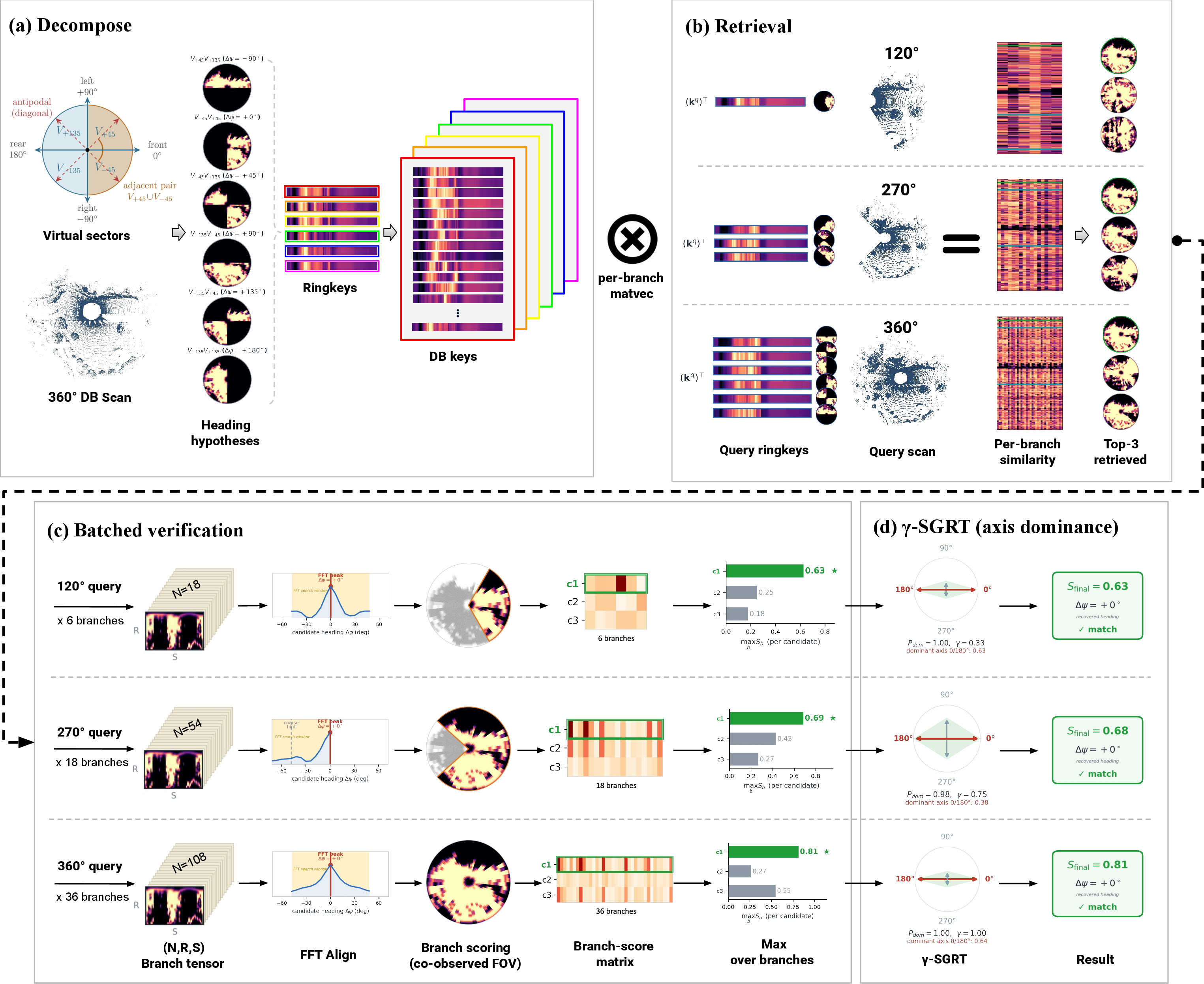
G-PROBE (Generalized PROBE) is a global localization system producing a metric SE(3) pose from a single query scan, extending the preliminary descriptor PROBE [11] from retrieval to arbitrary-FOV metric localization. The G-PROBE front-end (§4) performs cross-FOV ensemble retrieval and FOV-aware BKL scoring with SGRT aliasing suppression, exporting the BEV certainty map computed during scoring. The CG-GICP back-end (§5) consumes this map to restrict its fine refinement pass to reliably co-observed points (Fig. 2). The 6-DoF poses serve as one-shot initialization (kidnapped robot) or loop-closure constraints.

4 G-PROBE: Cross-FOV Ensemble Place Recognition↩︎
4.1 Virtual Sensor Decomposition↩︎
G-PROBE operates on ego-centric clouds (voxel downsampling). All fixed hyperparameters introduced below are collected with their values in Table ¿tbl:tab:params?. A revisit may approach from any heading \(\Delta\psi \in [0^\circ, 360^\circ)\), so when the merged azimuth \(\Phi_\text{total}\) is \(<360^\circ\), different sectors observe the same scene, and a heading-invariant system must handle all \(\Delta\psi\) without prior knowledge.
Definition 1 (Virtual Sensor Decomposition). Any sensor configuration with contiguous azimuthal coverage (single panoramic or gap-free multi-sensor array), yielding a merged ego-centric point cloud with total coverage \(\Phi_\text{total}\) (abbreviated \(\Phi\)) and center azimuth \(\phi_\text{base}\), is mathematically partitioned into \(N\) virtual sensors \(\{V_1, \ldots, V_N\}\) indexed by ascending center azimuth. Each virtual sensor is defined by its half-FOV \(\alpha = \Phi_\text{total} / (2N)\) and center azimuth \(\phi_i = \phi_\text{base} + (2i - N - 1) \cdot \alpha\). This decomposition is identity-preserving. The union of virtual FOVs exactly recovers the original coverage space, \(\bigcup_{i=1}^{N} [\phi_i - \alpha,\, \phi_i + \alpha] = [\phi_\text{base} - \Phi_\text{total}/2,\, \phi_\text{base} + \Phi_\text{total}/2]\).
This \(SE(2)\) abstraction decouples the pipeline from hardware. Points are assigned to virtual sensors \(V_i\) strictly by azimuth. Each virtual-sensor pair (below) encodes an explicit relative-heading hypothesis.
Instantiations. The number of virtual sensors follows the quantization rule \(N = \max(1, \mathrm{round}(\Phi_\text{total} / 90^\circ))\), a compute–resolution balance confirmed by ablation (§6.10). \(90^\circ\) sectors keep the \(O(N^4)\) cross-pair branch count (§[sec:retrieval]) within the real-time budget, so we fix \(N\) rather than tune it. A panoramic \(360^\circ\) LiDAR yields \(N{=}4\) sectors (\(\alpha = 45^\circ\)) centered at the inter-cardinal directions \(\phi_i \in \{\pm 45^\circ, \pm 135^\circ\}\). A \(270^\circ\) rig yields \(N{=}3\). Narrow-FOV LiDARs (e.g., Aeva \(120^\circ\), Avia \(70^\circ\)) resolve to \(N{=}1\), preserving the entire FOV as one structural template rather than sub-dividing it.
Pairwise decomposition. We decompose the virtual sensor array into all \(\binom{N}{2}\) pairwise subsets. Each virtual sensor pair \(P_{ij} = V_i \cup V_j\) has a union FOV mask \(\mathcal{F}_{ij}\) from the individual virtual sector coverages. For \(N=1\) (\(\binom{1}{2}=0\)), a single self-pair \(P_{11} \equiv V_1\) is matched against the opposing side’s \(\binom{N'}{2}\) pairs (its self-pair when \(N'{=}1\), with \(N'\) the database-side sector count), so the narrow-FOV sensor still participates in cross-heading matching. The center angle of pair \(P_{ij}\) is the circular mean \(\bar{\phi}_{ij} = \text{atan2}(\sin\phi_i + \sin\phi_j,\, \cos\phi_i + \cos\phi_j)\). For an antipodal pair (two opposite-facing sectors, e.g. the diagonal \(V_{+45}{\cup}V_{-135}\) in the \(N{=}4\) sensor), where the unit vectors cancel and the circular mean is undefined, we anchor \(\bar{\phi}_{ij}\) to the lower-indexed sector (for directly specified physical configurations with unequal sector FOVs, the narrower one).
Running example. The \(N{=}4\) sensor’s \(\binom{4}{2}{=}6\) pairs place the four adjacent pairs on the cardinal axes (front \(0^\circ\), left \(+90^\circ\), rear \(180^\circ\), right \(-90^\circ\)) and the two antipodal pairs on the diagonals (Fig. 3).
4.2 Stage 1: Density-Robust Retrieval↩︎
For each sensor pair \(P_{ij}\), we compute a \(D\)-dimensional L2-normalized retrieval key capturing the range-stratified structural statistics of the enclosed point cloud. The key reuses the probabilistic ring-key formulation of PROBE [11] (after Scan Context [2]). The novelty is not the key itself but its use per cross-FOV branch 4 –6 . The range axis is divided into \(N_r\) concentric annuli spanning \([0, R_{\max}]\). From the polar BEV grid (§4.3), each ring \(r \in \{1, \ldots, N_r\}\) produces two features: \[\boldsymbol{f}_r = [\bar{\mu}_r, \bar{z}_r]^{\top}\!,\; \bar{\mu}_r = \tfrac{1}{N_s}{\textstyle\sum_s}\mu(r,s),\; \bar{z}_r = \tfrac{1}{N_s}{\textstyle\sum_s}z_{\max}(r,s), \label{eq:ringfeat}\tag{1}\] where \(N_s\) is the number of azimuth bins of the polar BEV grid (§4.3), \(\bar{\mu}_r\) is the mean structural occupancy (from the polar-blurred \(\mu\), mitigating sensor-specific scanning patterns) and \(\bar{z}_r\) the mean structure height, which supports platforms of differing sensor height (ground vehicles, quadrupeds). Features are concatenated across rings into a \(D\)-dimensional vector (\(D = N_r \times 2\)) and globally L2-normalized, attenuating (without eliminating) the dependence of \(\bar{\mu}_r\) on absolute density, sufficient for cross-pair cosine retrieval.
Why cross-pair retrieval succeeds. The ring key is range-stratified, not azimuth-dependent. A revisit from a different heading sees the same structures through a different pair at the same ranges, keeping cross-pair cosine similarity meaningful. The compact key serves the \(O(M)\) search. The full polar BEV (§4.3) serves verification, cutting retrieval from \(O(M \cdot N_r \cdot N_s)\) to \(O(M \cdot D)\), \(D = 2N_r \ll N_r N_s\).
Cross-Pair Retrieval and Branch Generation. Given query node \(q\) and a database of \(M\) nodes, we generate all cross-pair branches by enumerating every \({(P_{ij}^{q}, P_{kl}^{\text{db}})}\) combination across query and database pairs. For each, the heading hint is the pair center angle difference: \[\Delta\psi_{\text{hint}} = \big(\bar{\phi}_{ij}^{q} - \bar{\phi}_{kl}^{\text{db}}\big) \bmod 360^\circ, \label{eq:hint}\tag{2}\] and the expected FOV overlap ratio is symmetrically normalized: \[w_{\text{FOV}} = \frac{|\mathcal{F}_{ij}^{q} \cap \text{roll}(\mathcal{F}_{kl}^{\text{db}}, \Delta\psi_{\text{hint}})|}{\min\!\left(|\mathcal{F}_{ij}^{q}|,\, |\text{roll}(\mathcal{F}_{kl}^{\text{db}}, \Delta\psi_{\text{hint}})|\right)}. \label{eq:fov95overlap}\tag{3}\] Here \(\text{roll}(\cdot,\Delta\psi)\) circularly shifts a mask by \({\mathrm{round}(\Delta\psi\, N_s/360^\circ)}\) azimuth bins. Normalized by the smaller FOV, the ratio measures the fraction of the usable observation that is shared, even under severe asymmetry (\(\text{DB}=90^\circ\), \(\text{Query}=360^\circ\)). A branch is retained only if \(w_{\text{FOV}} \geq w_{\min}\). Enumerating every pair makes reverse-heading revisits ordinary branches with \(\Delta\psi_{\text{hint}} \approx 180^\circ\), so no adjacency or reverse-branch logic is needed.
Symmetric FOV-overlap retrieval. For meaningful descriptor comparison under arbitrary FOV asymmetry, we restrict both query and database ring keys to their shared physical observation region (Fig. 3). For each branch \(b{=}(P_{ij}^{q}, P_{kl}^{\text{db}})\), writing \(\mathcal{F}_q{\equiv}\mathcal{F}_{ij}^{q}\), \(\mathcal{F}_\text{db}{\equiv}\mathcal{F}_{kl}^{\text{db}}\), and \(\Delta\psi_b{\equiv}\Delta\psi_{\text{hint}}\), the FOV overlap is computed per coordinate frame: \[\begin{align} \mathcal{O}_{q}(b) &= \mathcal{F}_{q} \cap \text{roll}(\mathcal{F}_{\text{db}},\, +\Delta\psi_b), \tag{4} \\ \mathcal{O}_{\text{db}}(b) &= \mathcal{F}_{\text{db}} \cap \text{roll}(\mathcal{F}_{q},\, -\Delta\psi_b), \tag{5} \end{align}\] where \(\mathcal{O}_{q}\) and \(\mathcal{O}_{\text{db}}\) represent the same physical region (up to the hint resolution \(\Delta\psi_b\)), expressed in the query and database frames respectively. The branch-specific retrieval keys are then: \[\begin{align} \boldsymbol{k}_{b}^{q} &= \text{RingKey}(\text{BEV}_{q} \odot \mathcal{O}_{q}), \nonumber \\ \boldsymbol{k}_{b}^{\text{db}} &= \text{RingKey}(\text{BEV}_{\text{db}} \odot \mathcal{O}_{\text{db}}). \label{eq:sym95ret} \end{align}\tag{6}\] Residual misalignment is corrected by the FFT cross-correlation of §[sec:alignment]. Database keys are pre-computed at insertion and stored in branch-specific matrices, so each branch performs its cosine search \(\boldsymbol{k}_{b}^{q} \cdot \boldsymbol{K}_{b}^{\text{db}}\) in \(O(M)\) at a constant-factor memory cost. When \(\mathcal{F}_{q} = \mathcal{F}_{\text{db}}\) both masks reduce to the full FOV and 6 degenerates to the unmasked ring key of PROBE [11].
Cross-sensor generalization. Eqs. 4 –6 depend only on the FOV masks \(\mathcal{F}\) (not on density, scan pattern, or modality), so the masking transfers unchanged across physically distinct sensors (e.g., a \(360^\circ\) spinning database vs.a \(70^\circ\) solid-state query), specified by their FOV extents (validated in §6.4).
Vote pooling and ranking. The top-\(k_b\) results per branch are pooled. For each database candidate \(m\), we record the FOV-weighted branch support and the cumulative similarity: \[v_{w}(m) = \sum_{b : m \in \text{top}_{k_b}(b)} w_{\text{FOV}}(b), \quad \bar{s}(m) = \sum_{b : m \in \text{top}_{k_b}(b)} \text{sim}_b(m), \label{eq:support95count}\tag{7}\] where \(w_{\text{FOV}}(b)\) is the branch’s FOV-overlap ratio, so low-overlap heading hypotheses are discounted consistently at both stages. A masked ring key spans fewer azimuth bins and casts a weaker vote at equal similarity. Candidates are ranked lexicographically by \((v_{w}(m), \bar{s}(m))\) (descending), and the top-\(K\) candidates advance to the geometric verification of §[sec:scoring]. The weighted support is a ranking signal only. False-positive rejection is left to the subsequent BKL scoring (§[sec:scoring]) and SGRT (§4.4).
Running example (cross-FOV, \(N{=}4 \to N{=}1\)). A panoramic database (\(N{=}4\), six pairs) queried by a narrow sensor (\(N{=}1\); e.g. Ouster\(\to\)Aeva) yields \(6\) branches. Whichever database pair faces the query’s true heading wins, and a reverse-direction query simply matches the rear (\(180^\circ\)) pair. FOV gating 3 down-weights pairs the narrow query cannot overlap. Two panoramic sensors give \(6{\times}6{=}36\) branches (Table ¿tbl:tab:ablation95NK?a).
Heading-Hypothesis Consistency Filtering. Branch results may be mutually inconsistent (a branch suggesting \(\Delta\psi \approx -90^\circ\) vs.one suggesting \(0^\circ\)). We quantize all branches into \(\lfloor 360^\circ / \Delta_{\text{step}} \rfloor\) heading hypotheses \(\{\mathcal{H}_\psi\}\) by each branch’s heading hint 2 , with \(\Delta_{\text{step}}{=}90^\circ\) the cardinal quantization step at which our virtual pairs align.
Each candidate \(m\) is scored only over the branches \(\mathcal{B}_m\) that nominated it, so incompatible heading evidence never mixes. The final heading is the winning branch of the max-over-branches aggregation (§[sec:scoring], using \(\max\) not mean to avoid bias from differing branch counts), while the hypothesis groups \(\{\mathcal{H}_\psi\}\) feed the SGRT uniqueness test (§4.4).
4.3 Stage 2: FOV-Aware Geometric Scoring↩︎
For geometric verification, each sensor pair constructs a polar BEV grid of size \(N_r \times N_s\) (\(N_r\) range rings, \(N_s\) azimuth bins), uniformly discretizing range \([0, R_{\max}]\) and the full \(360^\circ\) azimuth. Three grid channels are computed:
Occupancy \(\mu(r, s)\). Binary occupancy smoothed by an adaptive polar Gaussian blur. As derived in [11], marginalizing isotropic Cartesian translational uncertainty through the polar Jacobian yields, to first order, a distance-adaptive angular bandwidth \(\sigma_\theta \propto 1/r\), with a density-adaptive \(\sqrt{\rho}\) scaling (also from [11]) that prevents excessive dilation of isolated returns on sparse rings. The effective angular kernel width for a ring with occupancy density \(\rho(r)\) is: \[\sigma_\theta^{\text{grid}}(r) = \frac{\sigma_T \sqrt{\rho(r)}}{r \cdot \Delta_\theta}, \label{eq:adaptive95blur}\tag{8}\] where \(\sigma_T\) is the translational uncertainty, \(\rho(r)\) is the ring-level occupancy density (the fraction of occupied bins, computed on the raw, pre-blur occupancy), and \(\Delta_\theta = 2\pi/N_s\) is the angular bin width. The factor \(\sigma_T/(r\Delta_\theta)\) follows from an arc displacement \(\sigma_T\) subtending angle \(\sigma_T/r\) (radians); dividing by the bin width \(\Delta_\theta\) (radians per azimuth bin) renders \(\sigma_\theta^{\text{grid}}\) in grid-bin units. Completing the separable approximation, an analogous radial blur of width \(\sigma_r = \max(\mathrm{round}(\sigma_T/\Delta_r),\,1)\) bins (\(\Delta_r\) the ring width) is applied along the range axis. Retrieval is thereby robust to query–database translational offset, a property inherited from PROBE [11].
Bernoulli uncertainty \(\sigma(r, s) = \sqrt{\mu(1-\mu)}\). Used for shrinkage regularization.
Max-Height \(z_\text{max}(r,s)\). Structural signatures.
FOV-Aware Cross-Correlation Alignment. Cross-branch matches (e.g., the narrow query against the database’s left pair at \(\Delta\psi = +90^\circ\)) require aligning grids with different angular coverage. We define per-branch FOV masks \(\mathcal{F}_b\) and compute overlap: \[\mathcal{O}(b_q, b_\text{db}, \Delta s) = \mathcal{F}_{b_q} \cap \text{roll}(\mathcal{F}_{b_\text{db}}, \Delta s).\] Following the FFT-based rotation alignment of PROBE [11], cross-correlation on the max-height channel refines the heading. Our generalization restricts the correlation to the branch’s overlapping wedge and searches only the hint-centered window \(\mathcal{W}\) rather than the full \(360^\circ\) ring: \[\Delta s^* = \mathop{\mathrm{arg\,max}}_{\Delta s \in \mathcal{W}} \text{IFFT}\left[\sum_r \hat{Z}_q^{(r)} \cdot \overline{\hat{Z}_\text{db}^{(r)}}\right](\Delta s), \label{eq:fft95align}\tag{9}\] where \({\hat{Z}^{(r)} = \text{FFT}_s((z_{\max}\!\odot\mathcal{O})(r,\cdot))}\) is the DFT of ring \(r\)’s wedge-masked max-height row (\(\mathcal{O}\) fixed at the hint), \(\mathcal{W}\) is a narrow (\({\sim}{\pm}50^\circ\)) window around the branch-specific heading hint (the pairing geometry already constraining the heading to a sector), and the refined heading is \({\Delta\psi = \Delta s^{*}\, 360^\circ/N_s}\) (\(\Delta s^{*}\) already subsumes the hint).
Two-Factor BKL Scoring. After alignment, the verification score combines two factors, computed only within the overlapping FOV \(\mathcal{O}\) (the refined overlap wedge, extended over all rings):
Factor 1: Occupancy-Weighted Height CC. The height cross-correlation factor generalizes PROBE’s uncentered height cosine [11]. We weight it by the joint occupancy probability \(W = p_q p_\text{db}\) (the shrinkage occupancies defined in Factor 2) and mean-center the heights. Writing \(\tilde{z}_q = z_q - \bar{z}_q\) and \(\tilde{z}_\text{db} = z_\text{db} - \bar{z}_\text{db}\) for the \(W\)-mean-centered heights, \[\text{CC}_z = \max\!\left(0,\; \frac{\sum_{(r,s) \in \mathcal{O}} W\, \tilde{z}_q\, \tilde{z}_\text{db}}{\left\|\tilde{z}_q\right\|_W \, \left\|\tilde{z}_\text{db}\right\|_W}\right),\] where \(\left\|x\right\|_W = \big(\sum_{(r,s) \in \mathcal{O}} W\, x^2\big)^{1/2}\) is the \(W\)-weighted norm and \(\bar{z}_\bullet = \sum W z_\bullet / \sum W\) the \(W\)-weighted mean of each height, all sums running over the jointly height-observed cells of \(\mathcal{O}\) (both \(z_q\) and \(z_\text{db}\) nonzero). This is the standard \(W\)-weighted Pearson correlation, bounded in \([-1,1]\) by the Cauchy–Schwarz inequality, so the clamp yields \(\text{CC}_z \in [0,1]\); when fewer than five cells are jointly height-observed, the branch carries no height evidence and \(\text{CC}_z\) is defined as \(0\); if a valid overlap has vanishing weighted variance (constant height), the channel is uninformative and \(\text{CC}_z \triangleq 1\). The weighting \(W\) anchors the correlation on structure both sensors observe confidently (e.g., building walls), and the mean-centering cancels the shared ground level without any explicit ground segmentation. The \([0,1]\) clamp is deliberate. Negative correlation is no evidence of place identity and is treated as zero evidence, guaranteeing \(S_b \geq 0\) as the SGRT ratio 15 requires.
Factor 2: Bernoulli-KL Divergence. Each cell’s shrinkage occupancy \(p_i = \mu_i(1-\sigma_i) + \tfrac{1}{2}\sigma_i\) (the uncertainty-proportional shrinkage of [11]) pulls unreliable cells (\(\mu\!\approx\!0.5\), high \(\sigma\)) toward the uninformative \(0.5\), absorbing boundary and blur uncertainty. We rename PROBE’s Bernoulli-KL Jaccard \(\mathcal{J}_{KL}\) [11] to \(\mathrm{BKL}\) (Bernoulli-KL), omitting the imprecise “Jaccard.” The per-cell symmetric divergence between the two shrinkage occupancies is \[D_{\mathrm{sym}}(r,s) = \tfrac{1}{2}\!\left(\mathrm{KL}(p_q \| p_\text{db}) + \mathrm{KL}(p_\text{db} \| p_q)\right), \label{eq:dsym}\tag{10}\] where \(\mathrm{KL}(p \| q) = p \ln \tfrac{p}{q} + (1-p)\ln \tfrac{1-p}{1-q}\) is the Bernoulli KL divergence; \(D_{\mathrm{sym}}\) is non-negative by Gibbs’ inequality, computed uncoupled so it remains a genuine divergence between the measured occupancies.
Column-Wise Trimmed Aggregation. We aggregate the symmetric divergence over the co-observed cells \(\mathcal{U} = \{(r,s) \in \mathcal{O} : \mu_q(r,s) + \mu_\text{db}(r,s) > 0.1\}\), the occupancy soft-union within the FOV overlap \(\mathcal{O}\) (so \(\mathcal{U} \subseteq \mathcal{O}\)), as a column-trimmed mean. For each azimuthal column \(s\) we form the per-column mean divergence and its co-observed weight \[\begin{align} d_c(s) &= \frac{1}{W_c(s)}\sum_{r: (r,s) \in \mathcal{U}} D_{\mathrm{sym}}(r,s), \\[2pt] W_c(s) &= \big|\{\, r : (r,s) \in \mathcal{U} \,\}\big|. \end{align}\] Let \(\mathcal{S} = \{s \mid W_c(s) > 0\}\) with \(M_s = |\mathcal{S}|\). To reject dynamic obstacles or localized occlusion, which span several rings over a narrow angular range, we discard the \(\mathrm{round}(M_s \cdot \eta)\) highest-divergence columns (\(\eta \in [0,1)\)), keeping \(\mathcal{S}_{\text{kept}}\). The score is the co-observed-weighted average over the kept columns: \[\mathrm{BKL}= \exp\left(-\frac{\sum_{s \in \mathcal{S}_{\text{kept}}} W_c(s)\, d_c(s)}{\sum_{s \in \mathcal{S}_{\text{kept}}} W_c(s)}\right), \label{eq:bkl}\tag{11}\] where the trimmed set \(\mathcal{S}_{\text{kept}} \neq \emptyset\) (as \(\mathrm{round}(\eta M_s) < M_s\) at our \(\eta\) for any nonempty \(\mathcal{U}\)). Since the shrinkage occupancies are clipped to \([\epsilon, 1-\epsilon]\) (\(\epsilon{=}10^{-6}\)), \(D_{\mathrm{sym}}\) is finite and non-negative, and \(\mathrm{BKL}\in (0,1]\) without clamping. The trim is applied identically to all candidates.
Reduction to PROBE. With full co-visibility (where the co-observed mask \(\mathcal{U}\) specializes to PROBE’s soft union) and \(\eta = 0\), 11 reduces exactly to PROBE’s Bernoulli-KL Jaccard \(\mathcal{J}_{KL} = \exp\!\left(-\tfrac{1}{|\mathcal{U}|}\sum_{(r,s) \in \mathcal{U}} D_{\mathrm{sym}}(r,s)\right)\) [11], while the ensemble of branch-local windowed alignments spans all relative headings in place of PROBE’s single full-ring correlation (§1).
The per-branch score reuses the FOV overlap ratio \(w_{\text{FOV}}\) of 3 as a structural visibility prior. Branches with partial coverage (e.g., a \(90^\circ\) overlap out of \(180^\circ\)) are softly down-weighted, reflecting their reduced geometric information for verification: \[S_b = w_{\text{FOV}} \times \text{CC}_z \times \mathrm{BKL}. \label{eq:branch95score}\tag{12}\] The multiplicative two-factor structure (\(\text{CC}_z \times \mathrm{BKL}\)) follows PROBE’s \(\text{CC}_z \times \mathcal{J}_{KL}\) [11]. G-PROBE prepends the FOV-overlap prior \(w_{\text{FOV}}\), so on a homogeneous \(360^\circ\) pair (\(w_{\text{FOV}}{=}1\)) the score \(S_b\) recovers PROBE’s two-factor form. The multiplicative form enforces a veto. Disagreement in any single channel drives \(S_b\!\to\!0\), rejecting partial matches (e.g. urban canyons agreeing in height, \(\text{CC}_z{\approx}1\), but not occupancy, \(\mathrm{BKL}{\approx}0\)) that a weighted sum would over-score.
4.4 Probabilistic Softmax Gap Ratio Test (SGRT)↩︎
The final score rejects ambiguous matches by the dominance of the best heading axis over its competitors, via a Softmax over structural axes (antipodal-merged hypotheses) from a two-stage aggregation:
Stage 1: Hypothesis scoring (mean aggregation). Each hypothesis \(\mathcal{H}_\psi\) groups branches whose heading hints round to the same quantized angle. The hypothesis-level score is the arithmetic mean of its constituent branch scores: \[S_{\mathcal{H}_\psi} = \frac{1}{|\mathcal{H}_\psi|}\sum_{b \in \mathcal{H}_\psi} S_b. \label{eq:hyp95score}\tag{13}\] Branches that did not nominate \(m\) contribute \(S_b = 0\). Averaging, not maximizing, favors consensus within each heading direction, so one high-scoring branch cannot mask poor neighbors.
Stage 2: Antipodal axis grouping (max aggregation). A heading \(\psi\) and its \(180^\circ\) reverse describe the same line of travel, so we merge antipodal hypotheses into structural axes \(\mathcal{A}\) indexed by \(\psi \bmod 180^\circ\): \[\bar{S}_{\mathcal{A}} = \max_{\psi :\, \psi \bmod 180^\circ = \mathcal{A}} S_{\mathcal{H}_\psi}. \label{eq:axis95score}\tag{14}\] The maximum gives an axis full credit if either direction matches strongly, essential where both \(0^\circ\) and \(180^\circ\) score high (reverse-heading aliasing). In the running example the four hypotheses merge into \(|\mathcal{A}|{=}2\) structural axes \(\{0^\circ, 90^\circ\}\). SGRT tests dominance over the full axis set.
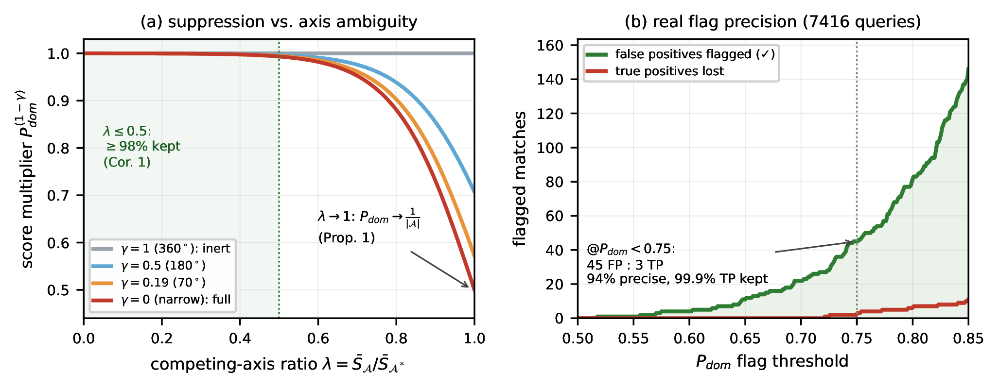
Adaptive Softmax. For score-scale invariance across sensor configurations and point-cloud densities, we employ an adaptive temperature \(\tau_\text{sm} = \bar{S}_{\mathcal{A}^*} / \kappa\), where \(\kappa > 0\) is a fixed sharpness constant (Fig. 4). Substituting into the standard Softmax yields a ratio-only expression: \[P_{dom} = \frac{1}{1 + \sum_{\mathcal{A} \neq \mathcal{A}^*} \exp\!\left(\kappa \cdot \left(\frac{\bar{S}_{\mathcal{A}}}{\bar{S}_{\mathcal{A}^*}} - 1\right)\right)}, \label{eq:softmax}\tag{15}\] where \(\mathcal{A}^* = \mathop{\mathrm{arg\,max}}_{\mathcal{A}} \bar{S}_{\mathcal{A}}\) (and \(P_{dom}\triangleq 1\) in the degenerate case \(\bar{S}_{\mathcal{A}^*}=0\), where no axis has support).
This probability \(P_{dom} \in (0, 1]\) is combined with an FOV coverage factor \(\gamma\) (the \(\gamma\)-adaptive exponent that names \(\gamma\)-SGRT) to produce the final similarity score: \[S_\text{final} = \left(\max_{b} S_b\right) \times P_{dom}^{\,(1-\gamma)}, \label{eq:race95score}\tag{16}\] where \(\gamma = \min(\Phi_q, \Phi_{\text{db}}) / 360^\circ \in [0, 1]\) measures the heading observability of the configuration, and \(\Phi_q, \Phi_{\text{db}}\) are the total azimuthal FOVs of the query and database sensors. The exponent \((1-\gamma)\) vanishes at \(\gamma = 1\) (panoramic: \({P_{dom}^{0}=1}\), since at full FOV a symmetric match still localizes to the correct place, so heading ambiguity no longer implies a wrong place and warrants no penalty; any residual heading symmetry is left to the back-end) and activates suppression for \(\gamma < 1\) in proportion to heading ambiguity (e.g., \(P_{dom}^{0.5}\) at \(180^\circ\), \(P_{dom}^{0.81}\) at \(70^\circ\)). The factorization keeps the best single-branch quality (\(\max_b S_b\)) while \(P_{dom}^{(1-\gamma)}\) independently penalizes heading ambiguity, so the axis-level averaging 13 never dilutes a strong branch. An aliased environment (symmetric intersections, four-way crossings) flattens the Softmax (\(P_{dom}\!\to\!1/|\mathcal{A}|\)) and suppresses \(S_\text{final}\), while a structurally unique scene (corners, T-junctions) drives \(P_{dom}\!\to\!1\) and preserves the geometric score.
SGRT generalizes Lowe’s ratio test [52] to all \(|\mathcal{A}|\) axes (not only the top two), with a scale-invariant continuous weight (not a binary accept–reject cut) and antipodal (forward–reverse) symmetry.
Proposition 1 (SGRT Suppression of Symmetric Aliasing). For a structurally symmetric environment in which \(|\mathcal{A}| \geq 2\) structural axes achieve identical scores \(S_0 > 0\), every ratio in 15 equals \(1\), so \(P_{dom} = 1/|\mathcal{A}|\) and \(S_\text{final} = (\max_b S_b)\,|\mathcal{A}|^{-(1-\gamma)} < \max_b S_b\) for any \(\gamma < 1\) (reducing to \((\max_b S_b)/|\mathcal{A}|\) at the narrow-FOV limit \(\gamma = 0\)), a strict attenuation independent of \(S_0\) and \(\kappa\).
Remark 1 (Minimum Conditions for SGRT). SGRT needs \(|\mathcal{A}| \geq 2\) structural axes, counted over the union of query and database pairs, so one wide side suffices. Against a \(70^\circ\) query (\(N{=}1\)), a \(360^\circ\) database (\(N{=}4\)) still spans multiple hypotheses and SGRT stays active. The \(\gamma\)-exponent further modulates this. At \(\gamma = 1\) (panoramic) SGRT is inactive regardless of \(|\mathcal{A}|\). Only when both sides are narrow-FOV (\(N = 1\) each, \(|\mathcal{A}| = 1\)) does \(P_{dom} = 1\) hold identically. There, the ensemble adds no aliasing-specific suppression and correctness rests on the raw BKL match score.
Corollary 1 (SGRT Non-Degradation of Unambiguous True Positives). For a true-positive match where the correct heading axis achieves score \(\bar{S}_{\mathcal{A}^*}\) and all other axes achieve scores \(\bar{S}_{\mathcal{A}} \leq \lambda \cdot \bar{S}_{\mathcal{A}^*}\) with \(\lambda < 1\), the SGRT attenuation is bounded: \[P_{dom} \geq \frac{1}{1 + (|\mathcal{A}|-1)\exp(\kappa(\lambda - 1))}. \label{eq:sgrt95bound}\tag{17}\] For \(|\mathcal{A}| = 2\) (e.g. a narrow query against a wide database), \(\kappa = 10\), \(\lambda \leq 0.5\), this gives \(P_{dom} \geq 0.993\). Even for a hypothetical \(|\mathcal{A}| = 4\) (the deployed axis set has \(|\mathcal{A}| \leq 2\)), \(P_{dom} \geq 0.980\). Since the applied multiplier satisfies \(P_{dom}^{(1-\gamma)} \geq P_{dom}\), SGRT preserves \(\geq 98\%\) of an unambiguous true positive’s score in the worst case (\(\gamma = 0\)), rising toward \(100\%\) as the FOV widens.
Proof. Every summand in 15 is at most \(\exp(\kappa(\lambda-1))\) by monotonicity. Substituting the \((|\mathcal{A}|-1)\)-term bound gives 17 . ◻
5 CG-GICP: Two-Stage Certainty-Guided Registration↩︎
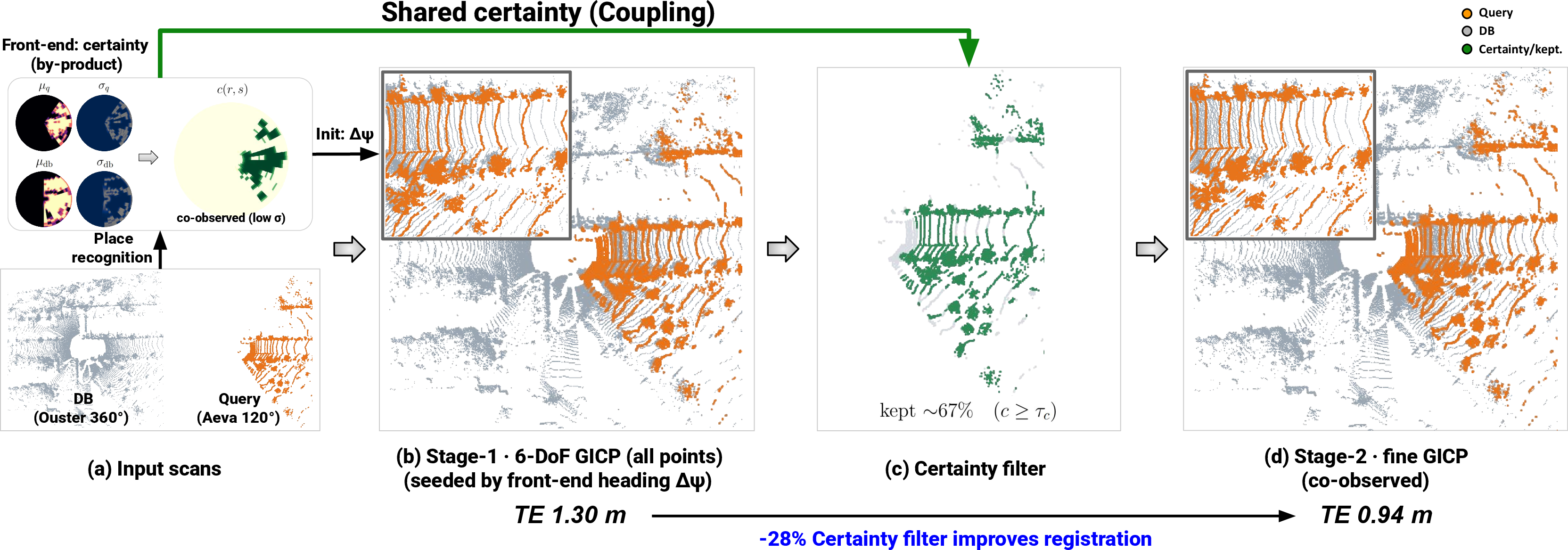
Standard ICP on FOV-constrained point clouds is biased by unreliable correspondences at FOV boundaries and in sparse, one-sided regions. CG-GICP addresses this with a coarse-to-fine two-pass Generalized-ICP coupled to the certainty map (§5.1–§5.3). This anchoring targets asymmetric-FOV and cross-sensor registration, where a large fraction of the query falls outside the database’s reliable observation. Fig. 5 runs the back-end end-to-end on a real cross-session, cross-sensor pair (KAIST06 Aeva \(120^\circ\) query, KAIST05 Ouster \(360^\circ\) database).
5.1 BEV Certainty Map Extraction↩︎
As a by-product of BKL scoring (§[sec:scoring]), the winning branch’s aligned grids yield a per-bin certainty weight \(c(r,s) \in [0,1]\): \[c(r,s) = w_{\text{cert}}(r,s) \cdot w_{\text{occ}}(r,s), \label{eq:certainty}\tag{18}\] where \(w_{\text{cert}}(r,s) = (1 - \sigma_q(r,s))(1 - \sigma_\text{db}(r,s))\) and \(w_{\text{occ}}(r,s) = \min(\mu_q(r,s), \mu_\text{db}(r,s))\) are the mutual certainty and mutual occupancy, zeroed outside the FOV overlap \(\mathcal{O}\) and where either scan has high uncertainty (\(\sigma > \sigma_{\text{thr}}\)) or low occupancy (\(\mu < \mu_{\text{thr}}\)). The weight is a conservative conjunction of two fuzzy t-norms, so only mutually well-observed bins score high.
Precise role of the certainty map. The certainty map does not encode structural distinctiveness. Clearly observed parallel boundaries receive \(c \approx 1\) despite their longitudinal degeneracy. Rather, it removes FOV-boundary, sparse, and high-uncertainty bins whose occupancy estimates would otherwise corrupt registration.
5.2 Certainty-Based Point Filtering↩︎
Each 3D point is projected to its polar BEV bin \((r_i, s_i)\) and assigned weight \(w_i = c(r_i, s_i)\). Points with \(w_i < \tau_c\) are discarded, typically removing 20–60% of the input (less on well-co-observed pairs) while keeping the reliably co-observed points. This filtering is asymmetric. Only the query (source) cloud is filtered, the target (database) cloud retained in full. The asymmetry ensures that for cross-heading matches (e.g., \(\Delta\psi = 180^\circ\)), target points outside the query’s filtered FOV remain valid correspondence targets, preventing empty-neighborhood artifacts in the KD-tree search.
5.3 Coarse-to-Fine Two-Pass Registration↩︎
Registration is initialized from G-PROBE’s refined heading \(\Delta\psi\), a median height offset \(\Delta z\), and zero lateral offset, then runs two Generalized-ICP passes.
Stage 1: Coarse GICP on all points. Generalized-ICP [38] is applied to the unfiltered source and target clouds: \[\begin{align} T_{\text{GICP}} = \mathop{\mathrm{arg\,min}}_T \sum_i &(p_i^{\text{tgt}} - T p_i^{\text{src}})^\top \\ \times &(C_i^{\text{tgt}} + T C_i^{\text{src}} T^\top)^{-1} (p_i^{\text{tgt}} - T p_i^{\text{src}}), \end{align} \label{eq:gicp}\tag{19}\] where \(C_i\) are the local surface covariance matrices. Using all points retains the broadest geometric constraints (particularly ground-plane and vertical structure constraining pitch, roll, and yaw) for a stable coarse pose \(T_{\text{GICP}}\) even on sparse sensors.
Stage 2: Certainty-filtered refinement. A second Generalized-ICP, initialized at \(T_{\text{GICP}}\), runs with the source restricted to its certainty-filtered points \(\mathcal{S}_c = \{i : c(r_i,s_i) \ge \tau_c\}\) (§5.2), matched against the full target: \[T_{\text{final}} = \mathop{\mathrm{arg\,min}}_{T} \sum_{i \in \mathcal{S}_c} \boldsymbol{e}_i(T)^\top \big(C_i^{\text{tgt}} + T C_i^{\text{src}} T^\top\big)^{-1} \boldsymbol{e}_i(T), \label{eq:gicp95fine}\tag{20}\] with residual \(\boldsymbol{e}_i(T) = p_i^{\text{tgt}} - T p_i^{\text{src}}\) and \(p_i^{\text{tgt}}\) the nearest neighbor of \(p_i^{\text{src}}\) under \(T\). Since the certainty map is zero outside the co-observed FOV overlap (§5.1), \(\mathcal{S}_c\) retains only co-observed points. Because the fine pass is initialized at \(T_{\text{GICP}}\), whose rotation is already well-constrained by the all-points coarse pass, it corrects mainly the residual translation and leaves the heading essentially unchanged.
Rationale for the two passes. A single all-points GICP admits one-sided FOV-edge bias; a filtered-only GICP loses the broad support needed for stable rotation on sparse sensors; the coarse-to-fine order resolves both (compared in §6.6, Table 4).
6 Experimental Evaluation↩︎
6.1 Datasets and Setup↩︎
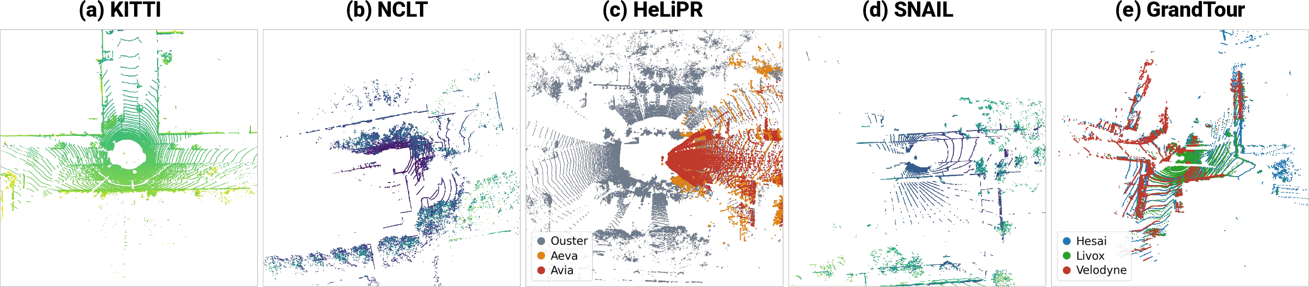
We evaluate on five datasets spanning three LiDAR modalities (mechanical spinning, solid-state, FMCW) and four robustness challenges (seasonal drift, extreme weather, cross-sensor, large-scale), each with a representative LiDAR scan in Fig. 6:
KITTI [53]: Sequences 00, 02, 05, and 08 (Velodyne HDL-64E, \(360^\circ\)). Sequence 08 provides reverse-heading loop closures. Sequences 00, 02, and 05 test scalability on diverse suburban environments.
NCLT [54]: Sequences 2012-05-26, 2012-08-20, 2012-09-28, and 2013-04-05 (Velodyne HDL-32E, \(360^\circ\), Segway): long-term dynamic change, repetitive structure, varied indoor–outdoor trajectories. Three multi-session pairs from 05-26 evaluate seasonal robustness.
HeLiPR [55]: KAIST05/06 and Riverside05/06, each with simultaneous Ouster OS2-128 (\(360^\circ\), mechanical spinning), Aeva Aeries-II (\(120^\circ\), FMCW), and Livox Avia (\(70^\circ\), solid-state), one synchronized cross-sensor benchmark.
SNAIL [56]: the Hesai XT32 (\(360^\circ\)) LiDAR of the SNAIL-Radar platform. Two challenge scenarios: (1) extreme weather (clear\(\to\)heavy rain, Starlake 2 km) and (2) long-term dynamic changes (46-day gap, Info Faculty 2.2 km).
GrandTour [57]: A quadruped (ANYmal-D) carrying three simultaneous \(360^\circ\)-azimuth LiDARs (Hesai XT32, 32-beam, \(120\,\text{m}\); Livox Mid-360, non-repetitive dome, \({\sim}40\,\text{m}\); and Velodyne VLP-16, 16-beam, \(100\,\text{m}\)) for the FOV-controlled cross-sensor study on a legged platform (§6.5), spanning an underground level (LEE-1), a rescue-training site (ARC-1), an alpine village (GRI-1), and a rail-yard re-localization pair (SBB-1\(\to\)2).
Baselines. We compare against ten methods spanning learning-free (M2DP [14], LiDAR Iris [15], SC [2], SC++ [3], SOLiD [8], RING++ [20], PROBE [11]) and deep learning (HeLiOS [5], BEVPlace++ [32], UniLGL [7]) approaches. The three deep baselines use their official pre-trained weights without domain adaptation. HeLiOS is trained on HeLiPR (DCC/KAIST/Riverside 04–06) across the same four LiDAR types including narrow-FOV scans, so its HeLiPR and limited-FOV results form an optimistic in-distribution bound, while its other results reflect genuine transfer. BEVPlace++ is trained on KITTI sequence 00, one of our four KITTI sequences, so its KITTI results partly reflect data seen during training. UniLGL is trained on MCD, a SNAIL-Radar route, and its Garden database, so our SNAIL cells share its training sensor. BEVPlace++ and UniLGL are applied zero-shot to HeLiPR with native pose estimators, with UniLGL’s official per-sensor windows (forward \([0,80]\) m for FOV-limited scans, centered for panoramic). Both rely on a fully-populated BEV grid (half-emptied under our asymmetric protocol), so we treat their asymmetric cross-FOV cells as an out-of-distribution generalization test.
Keyframe Selection. Database keyframes are sampled at \(5\,\text{m}\) spatial intervals and query keyframes at \(10\,\text{m}\) intervals.
Evaluation Protocol. A database keyframe is a ground-truth positive for a query iff it satisfies both (i) a Euclidean proximity threshold \(d_{\text{pos}} = 7.5\,\text{m}\) (identical for intra-sequence and multi-session), and (ii) a field-of-view (FOV) co-visibility criterion. The latter measures the angular intersection of the two scans’ azimuthal coverage arcs (each arc set by its sensor FOV and scan heading), normalized by the smaller of the two FOVs: \[\nu_{\text{cov}} \;=\; \frac{\,\angle\!\left[\,\mathrm{arc}(\Phi_q) \cap \mathrm{arc}(\Phi_{\text{db}})\,\right]}{\min\!\left(\Phi_q,\,\Phi_{\text{db}}\right)} \;\ge\; 0.25 . \label{eq:gt95covis}\tag{21}\] We normalize by the minimum FOV (intersection-over-minimum, not IoU). Under asymmetry the question is whether the narrower sensor’s view lies within the wider’s coverage. IoU would penalize the wider sensor’s unshared field. This fixes two conventional-ground-truth failures: distance-only metrics falsely accept oppositely-facing sensors, and heading-difference metrics over-penalize valid partial overlaps under high asymmetry (\(360^\circ\) vs.\(70^\circ\)). In the symmetric \(360^\circ\) case the criterion saturates (\(\nu_{\text{cov}} \equiv 1\)), reducing exactly to the conventional distance-only definition. Temporal exclusion uses \(d_{\text{exc}} = 20\,\text{m}\) trajectory distance.
Metrics. Following the standard top-1 loop-closure protocol of SC [2], SC++ [3], and RING++ [20], each query contributes a single decision (its top-1 retrieved match), accepted when its similarity exceeds a threshold \(\tau\). Sweeping \(\tau\) over the observed scores yields a precision–recall curve with \[\text{Precision} = \frac{\text{TP}}{\text{TP}+\text{FP}}, \qquad \text{Recall} = \frac{\text{TP}}{N_{\text{rev}}}, \label{eq:pr95metrics}\tag{22}\] where a true positive (TP) is an accepted top-1 satisfying the ground-truth criterion above, a false positive (FP) is any other accepted top-1 (including queries with no revisit), and \(N_{\text{rev}}\) is the total number of revisit queries. We report Recall@1 (R@1, the threshold-free top-1 success rate, \(\text{TP}_{\text{top1}}/N_{\text{rev}}\)), the maximum F1 along the curve, and AUC, the trapezoidal area under it. Since thresholds are drawn from the actual score distribution, AUC is invariant to monotone rescaling, a rank-based comparison across heterogeneous descriptors. All recall terms share the denominator \(N_{\text{rev}}\). AUC is our primary single-modality metric. For extreme cross-sensor settings (§6.4) we also emphasize Recall@1.
All G-PROBE and CG-GICP parameters are fixed across all experiments (Table ¿tbl:tab:params?).
6pt
@llll@
(lr)1-4 Voxel size & \(0.5\) m & \(\sigma_T\) & \(2\) m
Polar BEV \(N_r{\times}N_s\) & \(40{\times}60\) & top-\(K\) / branch-\(k_b\) & \(20\) / \(5\)
Max range & \(80\) m & Min FOV overlap \(w_{\min}\) & \(0.3\)
SGRT \(\kappa\) & \(10\) & Column-trim \(\eta\) & \(0.1\)
(lr)1-4 Max correspondence & \(2.0\) m & Certainty filter \(\tau_c\) & \(0.01\)
Certainty \(\sigma_{\text{thr}}\) & \(0.4\) & Certainty \(\mu_{\text{thr}}\) & \(0.15\)
Registration voxel & \(0.2\) m & Max iterations & \(30\)
6.2 Experiment 1: Standard LiDAR Place Recognition↩︎
Tables ¿tbl:tab:lidar95pr? and ¿tbl:tab:multisession95pr? evaluate 19 LiDAR configurations: 12 single-session sequences and 7 multi-session pairs spanning seasonal and long-term variations.
3.5pt
@ ll *11C @ & & & &
(lr)3-9 (lr)10-12 (lr)13-13 & & M2DP & Iris & SC & SC++ & SOLiD & RING++ & PROBE & HeLiOS\(^\dagger\) & BEVP++\(^\dagger\) & UniLGL\(^\dagger\) & G-PROBE
& R@1 & .624 & .875 & .737 & .844 & .780 & .865 & .917 & .748 & .980 & .885 & .881
& F1 & .601 & .670 & .689 & .769 & .677 & .485 & .840 & .662 & .928 & .655 & .766
& AUC & .568 & .660 & .644 & .753 & .661 & .412 & .832 & .604 & .950 & .655 & .749
& R@1 & .214 & .834 & .819 & .865 & .687 & .788 & .911 & .753 & .964 & .790 & .861
& F1 & .236 & .708 & .657 & .733 & .530 & .502 & .750 & .586 & .781 & .625 & .741
& AUC & .148 & .588 & .569 & .698 & .452 & .461 & .786 & .493 & .796 & .567 & .700
& R@1 & .650 & .713 & .808 & .863 & .682 & .863 & .878 & .796 & .878 & .726 & .865
& F1 & .638 & .671 & .738 & .841 & .558 & .667 & .789 & .732 & .819 & .666 & .802
& AUC & .578 & .630 & .716 & .812 & .514 & .653 & .804 & .611 & .818 & .538 & .780
& R@1 & .496 & .807 & .788 & .857 & .716 & .839 & .902 & .766 & .941 & .800 & .869
& F1 & .492 & .683 & .695 & .781 & .588 & .551 & .793 & .660 & .843 & .649 & .770
& AUC & .431 & .626 & .643 & .754 & .542 & .509 & .807 & .569 & .855 & .587 & .743
Sensors: KITTI Velodyne HDL-64E, NCLT Velodyne HDL-32E, HeLiPR Ouster OS2-128.
3.5pt
@ ll *11C @ & & & &
(lr)3-9 (lr)10-12 (lr)13-13 & & M2DP & Iris & SC & SC++ & SOLiD & RING++ & PROBE & HeLiOS\(^\dagger\) & BEVP++\(^\dagger\) & UniLGL\(^\dagger\) & G-PROBE
& R@1 & .452 & .744 & .724 & .726 & .517 & .536 & .787 & .807 & .917 & .736 & .779
& F1 & .472 & .795 & .722 & .728 & .486 & .512 & .792 & .781 & .871 & .725 & .811
& AUC & .390 & .693 & .644 & .656 & .365 & .381 & .751 & .709 & .873 & .666 & .742
& R@1 & .639 & .741 & .747 & .715 & .455 & .714 & .784 & .785 & .859 & .614 & .862
& F1 & .668 & .805 & .787 & .776 & .448 & .701 & .839 & .781 & .849 & .620 & .892
& AUC & .564 & .727 & .696 & .667 & .275 & .589 & .764 & .654 & .828 & .456 & .828
& R@1 & .800 & .954 & .953 & .927 & .809 & .500 & .956 & .922 & .989 & .913 & .949
& F1 & .813 & .968 & .957 & .938 & .808 & .500 & .964 & .922 & .988 & .915 & .952
& AUC & .768 & .953 & .949 & .923 & .734 & .498 & .953 & .898 & .988 & .890 & .935
& R@1 & .630 & .813 & .808 & .789 & .594 & .583 & .842 & .838 & .922 & .754 & .863
& F1 & .651 & .856 & .822 & .814 & .581 & .571 & .865 & .828 & .903 & .753 & .885
& AUC & .574 & .791 & .763 & .749 & .458 & .489 & .823 & .754 & .896 & .671 & .835
Sensors: NCLT Velodyne HDL-32E, HeLiPR Ouster OS2-128, SNAIL Hesai XT32.
In the symmetric, same-sensor single-session setting, the supervised BEVPlace++ leads across datasets, as expected for a descriptor trained on panoramic same-sensor driving data. Among learning-free methods, G-PROBE is competitive, at an average AUC of \(.743\), behind the learning-free leader SC++ (\(.754\)) and further behind PROBE (\(.807\)), with PROBE retaining a clear edge on KITTI. We attribute the gap to the ensemble structure. The aligned-pair divergence formula is exactly PROBE’s (§[sec:scoring]), and the ensemble’s windowed branch searches trade PROBE’s peak same-heading sensitivity for the heading diversity that cross-FOV matching demands. The ordering reverses where that diversity matters. Among learning-free methods G-PROBE leads on the multi-session average AUC (\(.835\) vs.\(.823\), driven by HeLiPR, Table ¿tbl:tab:multisession95pr?). G-PROBE’s advantages emerge under asymmetric FOV (Table ¿tbl:tab:sym95fov?) and cross-sensor heterogeneity (Table 2). RING++’s \(86.5\%\) R@1 on KITTI (Table ¿tbl:tab:lidar95pr?) confirms sound retrieval. Its lower AUC reflects the denser maps used here, over \(600\) frames each (vs.its original sparse \(20\) m map).
6.3 Experiment 2: Limited-FOV Robustness↩︎
A heading-invariant system must tolerate a reduced field of view.
Symmetric limited FOV. We first crop both database and query to the same limited FOV \(F \in \{180, 120, 90, 60\}^\circ\). The symmetric (top) block of Table ¿tbl:tab:sym95fov? reports mean Recall@1 and AUC over the single-session sequences. The learning-free baselines remain functional (AUC \(.16\)–\(.53\)), with G-PROBE and PROBE leading in AUC among learning-free methods at all FOVs. G-PROBE attains the best AUC overall (above even the supervised baselines) at \(120^\circ\) and \(90^\circ\), and is a close second at \(60^\circ\) (HeLiOS leads, \(.532\) vs.\(.485\)). Among supervised methods the Recall@1 lead splits by FOV width: BEVPlace++ at the wider \(\{180,120\}^\circ\), HeLiOS at the narrower \(\{90,60\}^\circ\). All methods remain functional.
Asymmetric FOV. We now introduce FOV asymmetry. The query is cropped from \(360^\circ\) down to \(60^\circ\) while the database stays at full \(360^\circ\), the regime a limited-FOV robot faces against a panoramic map. The asymmetric block of Table ¿tbl:tab:sym95fov? reports mean Recall@1 and AUC across the 12 single-session sequences of the three datasets. Fig. 1 visualizes the aggregate degradation. G-PROBE recovers the correct heading across the whole heading\(\times\)FOV space (not only same-/reverse-heading revisits), as the cross-sensor registration accuracy confirms (§6.6).
3.5pt
@ l *11C @ & & &
(lr)2-8 (lr)9-11 (lr)12-12 & M2DP & Iris & SC & SC++ & SOLiD & RING++ & PROBE & HeLiOS\(^\dagger\) & BEVP++\(^\dagger\) & UniLGL\(^\dagger\) & G-PROBE
\(180^\circ\) & 52.0 / .405 & 57.1 / .409 & 57.9 / .377 & 59.2 / .422 & 52.4 / .347 & 52.9 / .240 & 60.1 / .518 & 62.0 / .514 & 67.7 / .546 &
59.4 / .436 & 57.9 / .529
\(120^\circ\) & 53.0 / .407 & 62.0 / .405 & 66.1 / .353 & 64.9 / .401 & 61.7 / .337 & 50.5 / .236 & 67.2 / .526 & 68.5 / .567 & 70.6 / .527 & 63.0 /
.448 & 62.7 / .568
\(90^\circ\) & 49.8 / .347 & 60.0 / .379 & 70.5 / .330 & 71.0 / .371 & 53.8 / .321 & 47.2 / .207 & 66.4 / .497 & 70.7 / .559 & 69.9 / .482 & 63.6 / .415
& 62.6 / .560
\(60^\circ\) & 51.5 / .363 & 55.4 / .341 & 64.8 / .261 & 64.9 / .285 & 48.2 / .255 & 43.2 / .162 & 61.8 / .402 & 70.4 / .532 & 66.0 / .397 &
59.7 / .375 & 59.1 / .485
\(360^\circ\) & 49.6 / .431 & 80.7 / .626 & 78.8 / .643 & 85.7 / .754 & 71.7 / .542 & 83.8 / .509 & 90.2 / .807 & 76.6 / .569 & 94.1 / .855
& 80.0 / .587 & 86.9 / .743
\(180^\circ\) & 2.3 / .001 & 8.6 / .041 & 10.5 / .049 & 7.8 / .030 & 6.5 / .019 & 11.2 / .007 & 10.8 / .023 & 34.7 / .110 & 63.9 / .323 & 3.7 / .001 &
78.8 / .693
\(120^\circ\) & 1.2 / .000 & 4.7 / .025 & 6.0 / .030 & 3.9 / .015 & 2.6 / .005 & 5.3 / .002 & 4.5 / .009 & 24.7 / .064 & 40.8 / .163 & 2.4 / .000 &
73.6 / .623
\(90^\circ\) & 0.9 / .000 & 3.0 / .013 & 4.1 / .019 & 2.6 / .010 & 1.8 / .002 & 3.0 / .001 & 3.4 / .005 & 19.9 / .040 & 22.0 / .079 & 1.5 / .000 &
68.8 / .549
\(60^\circ\) & 0.8 / .000 & 2.3 / .008 & 2.9 / .011 & 1.8 / .008 & 1.6 / .003 & 2.5 / .000 & 2.2 / .002 & 14.1 / .023 & 9.3 / .034 & 0.7 / .000 &
53.7 / .382
\(\Delta\) (%) & \(-\)98.3% / \(-\)100.0% & \(-\)97.2% / \(-\)98.7% & \(-\)96.3% / \(-\)98.3% & \(-\)97.9% / \(-\)98.9% & \(-\)97.7% / \(-\)99.4% & \(-\)97.1% / \(-\)99.9% & \(-\)97.6% / \(-\)99.8% & \(-\)81.6% / \(-\)95.9% & \(-\)90.2% / \(-\)96.1% & \(-\)99.1% / \(-\)100.0% & \(-\)38.2% / \(-\)48.5%
| Ouster (\(360^\circ\)) | Aeva (\(120^\circ\)) | Avia (\(70^\circ\)) | |
|---|---|---|---|
| Single-Session (KAIST05 DB \(\to\) KAIST05 Query): Asymmetric FOV | |||
| Ouster (\(360^\circ\)) | |||
| HeLiOS\(^\dagger\): .718 / BEVP++\(^\dagger\): .962 / UniLGL\(^\dagger\): .720 / Ours: .862 | |||
| HeLiOS\(^\dagger\): .018 / BEVP++\(^\dagger\): .010 / UniLGL\(^\dagger\): .000 / Ours: .488 | |||
| HeLiOS\(^\dagger\): .028 / BEVP++\(^\dagger\): .002 / UniLGL\(^\dagger\): .000 / Ours: .329 | |||
| Aeva (\(120^\circ\)) | |||
| HeLiOS\(^\dagger\): .002 / BEVP++\(^\dagger\): .014 / UniLGL\(^\dagger\): .000 / Ours: .413 | |||
| HeLiOS\(^\dagger\): .859 / BEVP++\(^\dagger\): .843 / UniLGL\(^\dagger\): .495 / Ours: .873 | |||
| HeLiOS\(^\dagger\): .363 / BEVP++\(^\dagger\): .019 / UniLGL\(^\dagger\): .012 / Ours: .421 | |||
| Avia (\(70^\circ\)) | |||
| HeLiOS\(^\dagger\): .006 / BEVP++\(^\dagger\): .001 / UniLGL\(^\dagger\): .000 / Ours: .272 | |||
| HeLiOS\(^\dagger\): .424 / BEVP++\(^\dagger\): .042 / UniLGL\(^\dagger\): .004 / Ours: .422 | |||
| HeLiOS\(^\dagger\): .824 / BEVP++\(^\dagger\): .633 / UniLGL\(^\dagger\): .499 / Ours: .808 | |||
| Multi-Session (KAIST05 DB \(\to\) KAIST06 Query): Asymmetric FOV + Temporal Change | |||
| Ouster (\(360^\circ\)) | Aeva (\(120^\circ\)) | Avia (\(70^\circ\)) | |
| Ouster (\(360^\circ\)) | |||
| HeLiOS\(^\dagger\): .734 / BEVP++\(^\dagger\): .846 / UniLGL\(^\dagger\): .492 / Ours: .914 | |||
| HeLiOS\(^\dagger\): .006 / BEVP++\(^\dagger\): .006 / UniLGL\(^\dagger\): .000 / Ours: .508 | |||
| HeLiOS\(^\dagger\): .023 / BEVP++\(^\dagger\): .002 / UniLGL\(^\dagger\): .000 / Ours: .502 | |||
| Aeva (\(120^\circ\)) | |||
| HeLiOS\(^\dagger\): .018 / BEVP++\(^\dagger\): .020 / UniLGL\(^\dagger\): .000 / Ours: .411 | |||
| HeLiOS\(^\dagger\): .803 / BEVP++\(^\dagger\): .765 / UniLGL\(^\dagger\): .308 / Ours: .692 | |||
| HeLiOS\(^\dagger\): .517 / BEVP++\(^\dagger\): .026 / UniLGL\(^\dagger\): .021 / Ours: .412 | |||
| Avia (\(70^\circ\)) | |||
| HeLiOS\(^\dagger\): .018 / BEVP++\(^\dagger\): .003 / UniLGL\(^\dagger\): .000 / Ours: .224 | |||
| HeLiOS\(^\dagger\): .335 / BEVP++\(^\dagger\): .024 / UniLGL\(^\dagger\): .009 / Ours: .221 | |||
| HeLiOS\(^\dagger\): .834 / BEVP++\(^\dagger\): .707 / UniLGL\(^\dagger\): .469 / Ours: .749 | |||
The R@1 ranking mirrors the AUC ranking: mean off-diagonal R@1 per block (KAIST single/multi, Riverside single/multi) is \(43.9/42.1/30.1/24.9\%\) for G-PROBE vs.\(29.8/29.6/28.5/26.6\%\) for the strongest baseline (the in-distribution HeLiOS\(^\dagger\), which edges G-PROBE only in the Riverside multi-session block). All other baselines (PROBE next, up to \(21\%\)) stay below \(22\%\) in all four blocks.
Every learning-free baseline collapses under asymmetric FOV (\(-96\%\) or worse). Only G-PROBE remains reliable, even at extreme asymmetry (\(60^\circ\)). The symmetric block is the control: the same cropped FOVs, shared by both database and query, leave baselines functional (top block of Table ¿tbl:tab:sym95fov?). Their collapse under asymmetry (a cropped query against a panoramic database) therefore reflects the FOV asymmetry between query and database, not the FOV reduction itself.
6.4 Experiment 3: Cross-Sensor Generalization (HeLiPR)↩︎
We conduct an exhaustive cross-sensor evaluation over the three HeLiPR LiDARs with mutually overlapping fields of view (Ouster OS2-128 \(360^\circ\), Aeva Aeries-II \(120^\circ\), Livox
Avia \(70^\circ\)) in single-session (KAIST05) and multi-session (KAIST05\(\to\)06) configurations. We evaluate Mean AUC across all 9 sensor
combinations (\(3{\times}3\) matrix), comparing G-PROBE against the six baselines of Table 2. All methods operate at each sensor’s full native horizontal FOV.
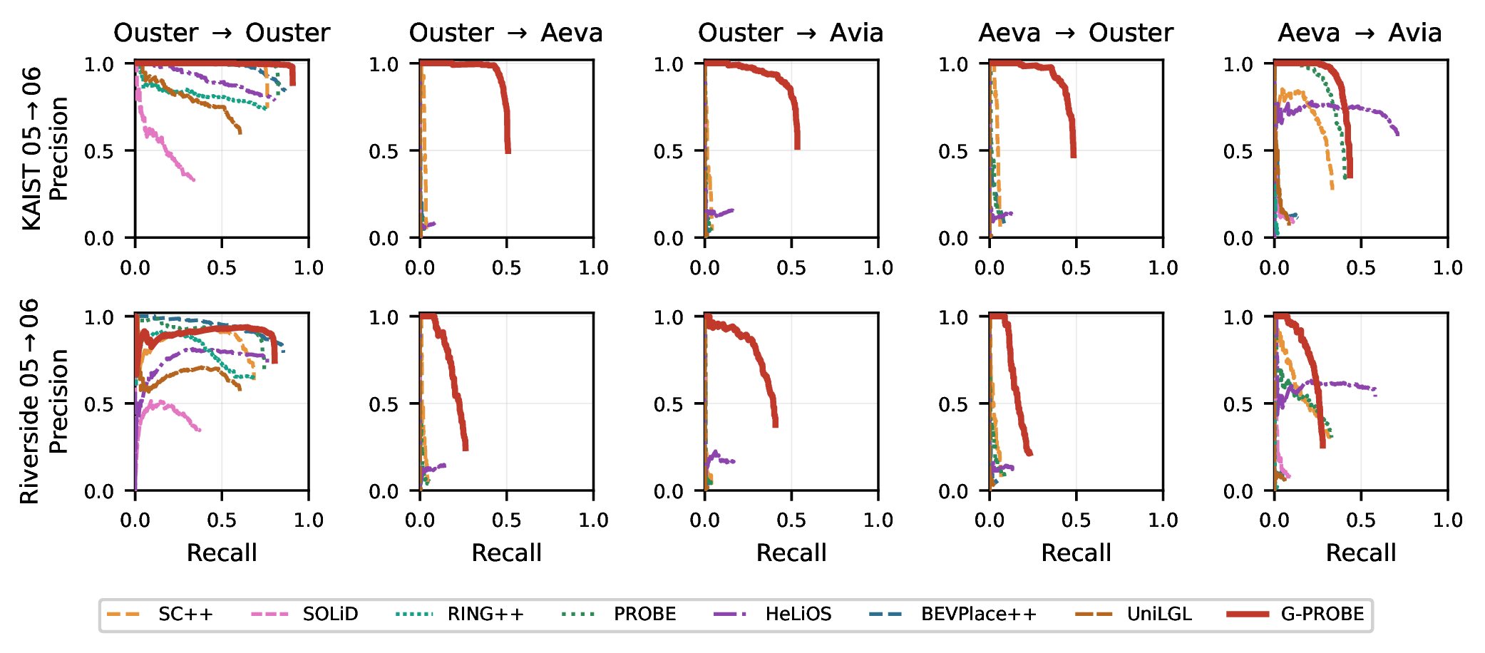
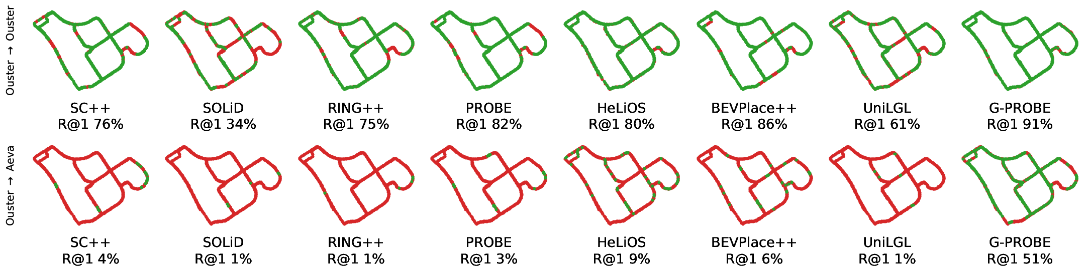
G-PROBE is the only method retaining non-trivial AUC across all off-diagonal cross-sensor pairs (Table 2). Its symmetric FOV-overlap formulation, Eqs. 4 –6 , restricts comparison to co-observed sectors.
The matrix separates into two regimes (Figs. 7 and 8). On the diagonal (same-sensor) all structurally-capable methods retain signal and G-PROBE is competitive (Ouster\(\to\)Ouster AUC \(.862\) vs.SC++ \(.859\)), though PROBE retains a slight edge across the single-session same-sensor diagonals and a larger one on the multi-session narrow-FOV diagonals. Off-diagonal, the ranking reverses. Pairing a \(360^\circ\) Ouster with a narrow-FOV sensor drives all evaluated learning-free and supervised baselines to near-zero AUC (\(\leq\!0.08\)). Their global descriptors penalize the unobserved field. G-PROBE alone retains usable similarity (Ouster\(\to\)Aeva \(.488/.508\), Ouster\(\to\)Avia \(.329/.502\) on KAIST single/multi-session, more than an order of magnitude above all baselines). The same trend holds on Riverside (Table 2 note, Table 5). By the same symmetric formulation, the reverse pairings keep signal (Fig. 7), though a wider-FOV database remains the stronger reference. The exception is the narrow-FOV pair (Aeva\(\leftrightarrow\)Avia), where in-distribution HeLiOS leads three of the four cells (e.g. multi-session Aeva\(\to\)Avia \(.517\) vs.\(.412\)) while G-PROBE takes the single-session Aeva\(\to\)Avia (\(.421\) vs.\(.363\)). Where sensors barely co-observe, all methods score near zero. G-PROBE’s scores are discounted by the \(w_{\text{FOV}}\) prior at minimal overlap rather than inflated.
6.5 Experiment 4: FOV-Controlled Cross-Sensor Study on a Legged Platform↩︎
In HeLiPR, FOV asymmetry and sensor heterogeneity are entangled. The GrandTour dataset [57] supplies the control that HeLiPR lacks: three simultaneously recorded LiDARs sharing a \(360^\circ\) azimuth yet differing in beam count, scan pattern, and range, so its cross-sensor cells isolate the density/pattern/range component alone. The platform is a quadruped (walking-induced roll/pitch), on which we apply G-PROBE zero-shot with parameters and protocol identical to HeLiPR (query keyframes at \(5\,\text{m}\) owing to the short missions). Table 3 spans four sites: three single-session (intra-mission loop closure: LEE-1, ARC-1, GRI-1) and one cross-mission re-localization (SBB-1\(\to\)SBB-2, 26 revisit queries per cell).
| Method | |||||||
| S / C | |||||||
| S / C | |||||||
| S / C | |||||||
| S / C | |||||||
| (mean) | |||||||
| (mean) | |||||||
| SC++ [3] | 26.4 / 20.8 | 61.1 / 39.8 | 44.9 / 29.4 | 67.9 / 35.9 | 50.1 | 31.5 | |
| SOLiD [8] | 26.4 / 29.9 | 50.0 / 25.0 | 38.9 / 28.5 | 50.0 / 22.4 | 41.3 | 26.5 | |
| RING++ [20] | 13.9 / 15.3 | 48.1 / 34.3 | 35.8 / 24.7 | 69.2 / 19.2 | 41.8 | 23.4 | |
| PROBE [11] | 22.2 / 26.4 | 63.0 / 51.9 | 44.9 / 44.7 | 67.9 / 34.6 | 49.5 | 39.4 | |
| HeLiOS\(^\dagger\) [5] | 44.4 / 31.9 | 44.4 / 35.2 | 46.3 / 39.3 | 59.0 / 28.2 | 48.5 | 33.7 | |
| BEVP++\(^\dagger\) [32] | 37.5 / 27.8 | 70.4 / 49.1 | 63.2 / 39.9 | 75.6 / 27.6 | 61.7 | 36.1 | |
| UniLGL\(^\dagger\) [7] | 30.6 / 33.3 | 61.1 / 51.9 | 43.4 / 29.2 | 56.4 / 24.4 | 47.9 | 34.7 | |
| G-PROBE (Ours) | 23.6 / 22.2 | 61.1 / 55.6 | 55.6 / 50.7 | 66.7 / 32.7 | 51.8 | 40.3 |

With the FOV shared, the zero-shot supervised baselines that fell to near zero on HeLiPR’s cross-sensor cells (BEVPlace++, UniLGL; Table 2) recover (up to \(49\)–\(52\%\) R@1 on the strongest site, ARC-1, and \(35\)–\(36\%\) cross-sensor mean), indicating that FOV asymmetry, not heterogeneity per se, causes their collapse. Under cross-mission re-localization their scores drop again (\(27.6/24.4\%\)), and the ordering flips (SC++ \(35.9\), PROBE \(34.6\), G-PROBE \(32.7\%\)). Fig. 9 shows one such cell (Hesai\(\to\)Velodyne), G-PROBE re-localizing zero-shot across a 32-to-16-beam gap. With the retrieval-shortlist baselines depth-matched to G-PROBE (\(K{=}20\)), G-PROBE leads on the cross-sensor mean (\(40.3\%\), Table 3), including the strongest cross-sensor cell (ARC-1, \(55.6\%\)), and is competitive on the same-sensor control (except the underground LEE-1, which the supervised baselines lead). Over the \(27\) single-session cells of the three sites, G-PROBE leads the learning-free methods (\(44.1\%\) vs.PROBE \(41.8\%\) and SC++ \(34.7\%\)). The supervised baselines reach \(45.0\%\) (BEVPlace++), \(40.4\%\) (UniLGL), \(38.7\%\) (HeLiOS, out-of-distribution here), placing G-PROBE second overall, \(0.9\) percentage points (pp) behind BEVPlace++.
| KAIST \(\to\) Aeva (\(120^\circ\)), \(n{=}623\) | KAIST \(\to\) Avia (\(70^\circ\)), \(n{=}618\) | Riverside \(\to\) Aeva (\(120^\circ\)), \(n{=}604\) | Riverside \(\to\) Avia (\(70^\circ\)), \(n{=}604\) | |||||||||
|---|---|---|---|---|---|---|---|---|---|---|---|---|
| 2-4 (lr)5-7 (lr)8-10 (lr)11-13 Method | TE\(_{50/95}\) | RE\(_{50/95}\) | Succ. | TE\(_{50/95}\) | RE\(_{50/95}\) | Succ. | TE\(_{50/95}\) | RE\(_{50/95}\) | Succ. | TE\(_{50/95}\) | RE\(_{50/95}\) | Succ. |
| P2P-ICP | 0.79 / 1.23 | 1.93 / 3.00 | 97.0% | 0.68 / 2.38 | 1.62 / 3.30 | 93.9% | 0.77 / 1.97 | 1.89 / 3.52 | 92.9% | 0.63 / 4.27 | 1.91 / 3.59 | 84.4% |
| GICP | 0.72 / 1.15 | 1.85 / 2.57 | 97.9% | 0.81 / 1.18 | 1.42 / 2.02 | 97.2% | 0.75 / 1.89 | 1.85 / 2.36 | 93.5% | 0.79 / 1.69 | 1.49 / 1.75 | 94.2% |
| KISS-ICP | 0.73 / 1.15 | 1.79 / 2.50 | 97.0% | 0.81 / 2.94 | 1.42 / 2.44 | 92.1% | 0.77 / 2.33 | 1.80 / 4.68 | 91.1% | 0.82 / 2.48 | 1.50 / 2.25 | 90.2% |
| GICP 2-Stage\(^{\S}\) | 0.72 / 1.15 | 1.85 / 2.57 | 97.9% | 0.81 / 1.18 | 1.42 / 2.02 | 97.2% | 0.75 / 2.20 | 1.85 / 2.33 | 93.4% | 0.79 / 1.77 | 1.49 / 1.75 | 94.2% |
| CG 1-Stage | 0.75 / 1.17 | 1.85 / 2.74 | 97.0% | 0.83 / 1.34 | 1.46 / 2.33 | 95.8% | 0.76 / 2.33 | 1.84 / 2.59 | 92.5% | 0.82 / 1.84 | 1.49 / 1.93 | 94.4% |
| CG 2-Stage | 0.74 / 1.14 | 1.85 / 2.58 | 98.6% | 0.83 / 1.17 | 1.45 / 2.18 | 97.2% | 0.76 / 1.75 | 1.84 / 2.42 | 94.0% | 0.82 / 1.61 | 1.49 / 1.82 | 94.7% |
3.0pt
On the same-sensor reference (Ouster\(\to\)Ouster, both sites, \(n{=}620/604\)) all variants nearly coincide (TE\(_{50}\) within \(0.03\) m, success \(98.2\)–\(99.5\%\), except KISS-ICP’s Riverside tail at \(95.9\%\)). Averaged over the four cross-sensor blocks: Success \(=\) P2P \(92.0\), GICP \(95.7\), GICP 2-Stage\(^{\S}\) \(95.7\), KISS \(92.6\), CG-GICP 1-Stage \(94.9\), 2-Stage \(\mathbf{96.1}\); TE\(_{95}\) (m) \(=\) P2P \(2.5\), GICP \(1.5\), GICP 2-Stage\(^{\S}\) \(1.6\), KISS \(2.2\), 1-Stage \(1.7\), 2-Stage \(\mathbf{1.4}\); RE\(_{95}\) (\(^\circ\)) \(=\) GICP \(\mathbf{2.2}\) (best), 2-Stage \(2.2\). \(^{\S}\) Control: coarse pass \(+\) all-points fine pass, without the certainty filter. It reproduces plain GICP on the KAIST blocks (TE\(_{95}\) unchanged at \(1.15\) and \(1.18\) m) and regresses on the harder Riverside blocks (TE\(_{95}\) \(1.89{\to}2.20\) and \(1.69{\to}1.77\) m). The \(^{\S}\) control row is excluded from the bold/underline ranking.
6.6 Experiment 5: Cross-Sensor Geometric Registration↩︎
We evaluate metric registration on cross-sensor loop-closure pairs: an Ouster \(360^\circ\) database against Aeva \(120^\circ\) and Avia \(70^\circ\) queries on both HeLiPR sites, multi-session (\(05\to06\)). Each query is paired with its nearest database keyframe within \(10\,\text{m}\) (distance-only, without the co-visibility gate of 21 ), assessing all genuine revisits regardless of FOV overlap. The cross-day protocol is essential, since co-located single-session pairs leave the heading initialization near ground truth and all refiners appear near-perfect. All methods (P2P-ICP [37], GICP [38], KISS-ICP [40]) receive identical G-PROBE initialization (yaw, \(\Delta z\)) and correspondence distance (\(2.0\,\text{m}\)), both clouds voxel-downsampled to \(0.2\,\text{m}\), isolating the refinement stage. The experiment doubles as the CG-GICP architecture ablation: GICP \(=\) coarse pass only, 1-Stage \(=\) certainty-filtered fine pass only, 2-Stage \(=\) both. Table 4 reports the results.
On the same-sensor Ouster\(\to\)Ouster reference (see the note to Table 4), all variants nearly coincide, so the differences below emerge only once full co-visibility is lost. Under cross-sensor asymmetry the methods separate not in the typical case (median \(\text{TE}_{50}\approx 0.6\)–\(0.8\,\text{m}\) for all) but in the worst-case tail. As the query FOV narrows, P2P-ICP’s and KISS-ICP’s \(\text{TE}_{95}\) grow to \(2.4\)–\(4.3\,\text{m}\) (unconstrained where the sensors do not co-observe), pulling success down to \(84.4\)–\(97.0\%\). Certainty-guided filtering then tightens the residual tail: 2-Stage reaches the best average success (\(96.1\%\)) and the tightest worst-case translation (\(\text{TE}_{95}=1.4\,\text{m}\)). Most of the gain over P2P-ICP comes from the GICP optimizer itself. The co-visibility filter supplies the final worst-case-tail tightening (\(\text{TE}_{95}\,1.5\!\to\!1.4\,\text{m}\)). Within the two-pass architecture, the tail tightening is attributable to the certainty filter: the GICP 2-Stage\(^{\S}\) control (the same coarse-to-fine pass without the certainty filter) does not tighten the tail (Table 4, note), since re-optimizing over the uncertain FOV-boundary correspondences re-introduces their bias. Only filtering them out does. The alignment is visualized end-to-end in Fig. 5.
Between the two CG-GICP architectures the 2-Stage scheme is the stronger default (with the best success in all cross-sensor blocks). The coarse pass supplies broad constraints that stabilize the heading before the certainty-filtered fine pass. On the voxel-downsampled registration clouds the coarse pass does not perturb the translation under extreme asymmetry. In the harder Riverside blocks the gap is largest (Riverside-Aeva: 2-Stage \(\text{TE}_{95}=1.75\,\text{m}\) versus \(2.33\,\text{m}\) for 1-Stage). We retain both as configurable variants.
6.7 Experiment 6: End-to-End Metric Global Localization↩︎
| Ouster (\(360^\circ\)) | Aeva (\(120^\circ\)) | Avia (\(70^\circ\)) | |
|---|---|---|---|
| KAIST05 DB \(\to\) KAIST06 Query (cross-day) | |||
| Ouster (\(360^\circ\)) | |||
| G-PROBE (w/o CG) 90.5/0.37/0.2 G-PROBE (CG) 91.5/0.36/0.2 | |||
| G-PROBE (w/o CG) 49.2/0.72/1.9 G-PROBE (CG) 50.3/0.71/1.9 | |||
| G-PROBE (w/o CG) 53.4/0.84/1.4 G-PROBE (CG) 55.0/0.83/1.4 | |||
| Aeva (\(120^\circ\)) | |||
| G-PROBE (w/o CG) 39.2/0.63/1.8 G-PROBE (CG) 40.6/0.62/1.8 | |||
| G-PROBE (w/o CG) 65.5/0.32/0.3 G-PROBE (CG) 66.0/0.31/0.3 | |||
| G-PROBE (w/o CG) 41.1/0.86/2.1 G-PROBE (CG) 41.4/0.86/2.1 | |||
| Avia (\(70^\circ\)) | |||
| G-PROBE (w/o CG) 28.6/0.71/1.5 G-PROBE (CG) 29.1/0.71/1.4 | |||
| G-PROBE (w/o CG) 21.5/0.94/2.2 G-PROBE (CG) 21.8/0.94/2.2 | |||
| G-PROBE (w/o CG) 78.7/0.39/0.2 G-PROBE (CG) 79.8/0.39/0.2 | |||
| Riverside05 DB \(\to\) Riverside06 Query (cross-day) | |||
| Ouster (\(360^\circ\)) | |||
| G-PROBE (w/o CG) 80.4/0.17/0.1 G-PROBE (CG) 82.1/0.17/0.1 | |||
| G-PROBE (w/o CG) 24.8/0.81/1.8 G-PROBE (CG) 25.4/0.81/1.8 | |||
| G-PROBE (w/o CG) 42.0/0.82/1.5 G-PROBE (CG) 42.2/0.82/1.5 | |||
| Aeva (\(120^\circ\)) | |||
| G-PROBE (w/o CG) 21.9/0.58/1.7 G-PROBE (CG) 22.4/0.58/1.7 | |||
| G-PROBE (w/o CG) 47.3/0.21/0.2 G-PROBE (CG) 47.8/0.21/0.2 | |||
| G-PROBE (w/o CG) 29.6/0.86/2.1 G-PROBE (CG) 29.9/0.86/2.1 | |||
| Avia (\(70^\circ\)) | |||
| G-PROBE (w/o CG) 15.8/0.65/1.5 G-PROBE (CG) 16.3/0.64/1.5 | |||
| G-PROBE (w/o CG) 15.0/0.90/2.2 G-PROBE (CG) 15.7/0.88/2.2 | |||
| G-PROBE (w/o CG) 58.8/0.27/0.2 G-PROBE (CG) 59.4/0.27/0.2 | |||
\(\dagger\): supervised (deep-learned). Diagonal \(=\) same-sensor (loop-closure). Off-diagonal \(=\) cross-sensor. The TE/RE medians are conditioned on each method’s correctly-retrieved set, whose size varies by more than an order of magnitude across methods (e.g.on Ouster\(\to\)Avia, SC++ retrieves \({\sim}20\) pairs vs.G-PROBE’s \({\sim}370\)). A low-recall baseline’s median therefore reflects only its few easiest retrievals, so Success, which conjoins retrieval and pose, is the unbiased metric.
Having isolated retrieval (§6.4) and registration (§6.6), we now evaluate the complete system. Given a query scan, each method must retrieve a database candidate and recover a 6-DoF metric pose. A query is a localization success only if its top-1 retrieval satisfies the ground-truth positive criterion 21 and the pose is within \(2\,\text{m}\) and \(5^\circ\) of ground truth. The rate is reported over all revisit queries (the Recall@1 denominator).
Following UniLGL’s [7] global localization benchmark, each method runs its native pose estimator rather than a forced common back-end: UniLGL [7] via its GNC-TLS solver without additional registration; SC++ [3] is semi-metric (1-DoF yaw via aligning-key shift) and pairs with GICP, its prescribed ICP-family refinement, initialized by that yaw; G-PROBE uses its 2-Stage CG-GICP. Because the success metric scores a 6-DoF pose, methods that emit only a 3-DoF planar pose (BEVPlace++ [32], RING++ [20]) or no metric pose at all (the retrieval-only descriptors) cannot be scored end-to-end and appear at the place recognition level only (Tables ¿tbl:tab:lidar95pr?, ¿tbl:tab:multisession95pr?, 2). Table 5 reports the full \(3{\times}3\) database\(\times\)query matrix.
On the diagonal (same-sensor), G-PROBE attains the best success on both Ouster\(\to\)Ouster blocks (\(91.5\%\)/\(82.1\%\) on KAIST/Riverside) and is competitive on the narrow diagonals (G-PROBE leads KAIST Avia, \(79.8\%\) vs.SC++ \(71.3\%\), while SC++ leads the other three by \(\le\!10\) pp). Off-diagonal, the gap is pronounced. Baselines on the Ouster-paired cells already collapse at retrieval (success \(0\)–\(7\%\)), the heading essentially unconstrained for the rare retrieved query (UniLGL median rotation \(164.7^\circ\) on Ouster\(\to\)Aeva), whereas G-PROBE both finds the place and recovers an accurate metric pose, reaching \(55.0\%\)/\(0.83\,\text{m}\)/\(1.4^\circ\) on KAIST Ouster\(\to\)Avia and \(50.3\%\) on Ouster\(\to\)Aeva, against \(\leq\!4.9\%\) for all baselines, a \(10\)–\(13\times\) gap over the best baseline. The same dominance holds on Riverside (\(16\)–\(42\%\) vs.\(\leq\!5.3\%\)). Only Aeva\(\leftrightarrow\)Avia leaves a baseline partly functional (SC++ \(16\)–\(32\%\), ahead on one Riverside cell). A strong pose estimator cannot compensate for a query never retrieved, so on the wide\(\leftrightarrow\)narrow pairings G-PROBE alone succeeds end-to-end. CG-GICP nonetheless matches or exceeds plain GICP in all \(18\) cells (mean \(+0.7\) pp).
6.8 Ablation Study: Column-Trimmed Aggregation↩︎
This ablation isolates the column-trim \(\eta\) (§[sec:scoring], 11 ), the robustness step that discards the \(\eta{=}10\%\) highest-divergence azimuth columns before aggregation. Holding all other components fixed, we sweep \(\eta\in\{0,0.05,0.1,0.2,0.3\}\) (Table ¿tbl:tab:ablation95obs?a) on the HeLiPR multi-session (\(05{\to}06\)) cells of both sites, where cross-day dynamic content differs most.
| Column-trim \(\eta\) | Same-sensor | Cross-sensor |
|---|---|---|
| \(0\) (no trim) | .672 | .272 |
| \(0.05\) | .678 | .282 |
| \(\mathbf{0.1}\) (default) | .677 | .282 |
| \(0.2\) | .677 | .289 |
| \(0.3\) | .677 | .292 |
| Match group | Queries | Correct (TP) % |
|---|---|---|
| Confident (\(P_{dom} \geq 0.9\)) | \(7{,}141\) (\(96.3\%\)) | \(30.3\) |
| SGRT-flagged (\(P_{dom} < 0.9\)) | \(275\) (\(3.7\%\)) | \(6.2\) |
4.5pt (a)
(b)
The cross-FOV decomposition and FOV masking already provide the cross-sensor robustness. The symmetric BKL (PROBE’s divergence under the decomposition) reaches \({\sim}0.38\) AUC on KAIST’s wide\(\leftrightarrow\)narrow cells (Table 2), where all external baselines drop to near-zero. The column-trim adds a further small, near-tuning-free gain. Pooled over both sites, the \(0{\to}0.05\) trim raises the cross-sensor mean AUC by \({+}0.010\) (same-sensor \({+}0.006\)) by rejecting the worst dynamic-object/occlusion columns, and the score then stays within a narrow band for \(\eta\in[0.05,0.3]\) (cross-sensor rising a further \({\sim}{+}0.01\) to its \(\eta{=}0.3\) maximum, Table ¿tbl:tab:ablation95obs?a). Recall@1 is essentially unchanged (the ranking set by the decomposition). The effect is largest on the wide\(\leftrightarrow\)narrow cross-sensor cells (e.g.\({+}0.05\) AUC on KAIST Aeva\(\to\)Ouster), where a few dynamic-object or occlusion columns would otherwise penalize a genuine match. The same-sensor effect is smaller, as static panoramic revisits carry little transient disagreement.
6.9 Ablation Study: SGRT↩︎
SGRT down-weights a match by its heading-uniqueness probability \(P_{dom}\) 15 , suppressing heading aliasing. Such aliasing arises in rotationally near-symmetric scenes (open plazas, four-way intersections, feature-poor stretches), uncommon in HeLiPR’s directional driving. SGRT therefore substantially down-weights only \({\sim}3.7\%\) of revisit queries and leaves aggregate retrieval metrics essentially unchanged. The meaningful question is thus calibration rather than aggregate effect: whether the matches SGRT flags (\(P_{dom}\) low) are the unreliable ones. Table [tbl:tab:ablation95sgrt](b) answers this. Fig. 4 (b) visualizes the calibration.
The point-biserial correlation \(\rho(P_{dom},\mathrm{TP}) = +0.15\) (\(p < 10^{-36}\)) confirms the signal. SGRT flags matches several times less likely to be correct (\(6.2\%\) vs.\(30.3\%\)): e.g., a cross-session KAIST Ouster(\(360^\circ\))\(\to\)Aeva(\(120^\circ\)) query whose aliased top-1 lies \(84\,\text{m}\) from the true revisit scores comparably across its dominant heading axes, so the flattened Softmax (\(P_{dom}{=}0.67\)) drives it below threshold. Disabling it shifts aggregate precision–recall within noise, and the score-scale-invariant ratio 15 gives identical results for \(\kappa\in\{10,15,20\}\).
6.10 Hyperparameter Ablations: Sector Count \(N\) and Retrieval Depth \(K\)↩︎
| sector | Ouster\(\to\)Ouster (pano.) | Ouster\(\to\)Aeva (cross-FOV) | |||||
|---|---|---|---|---|---|---|---|
| 3-5(lr)6-8 \(N\) | (\(^\circ\)) | R@1 | AUC | \(\#b\) | R@1 | AUC | \(\#b\) |
| 1 | 360 | 45.6 | .385 | 1 | 26.0 | .250 | 1 |
| 2 | 180 | 45.6 | .385 | 1 | 1.7 | .007 | 1 |
| 3 | 120 | 66.6 | .595 | 9 | 31.3 | .275 | 3 |
| 4 | 90 | 88.6 | .862 | 36 | 52.0 | .488 | 6 |
| 6 | 60 | 90.8 | .858 | 189 | 46.7 | .425 | 15 |
| 8 | 45 | 87.2 | .750 | 528 | 51.1 | .475 | 28 |
| Query \(360^\circ\) (pano.) | Query \(120^\circ\) | Query \(90^\circ\) | ||||
|---|---|---|---|---|---|---|
| 2-3(lr)4-5(lr)6-7 \(K\) | R@1 | AUC | R@1 | AUC | R@1 | AUC |
| 10 | 86.1 | .841 | 64.3 | .637 | 60.8 | .598 |
| 20 | 88.6 | .862 | 74.4 | .732 | 70.7 | .690 |
| 30 | 89.2 | .867 | 75.0 | .737 | 71.0 | .692 |
(a)
(b)
Virtual-sector count \(N\). The sector count is fixed by \(N{=}\max(1,\mathrm{round}(\Phi/90^\circ))\) (§4.1), not tuned. Overriding it on two HeLiPR KAIST05 cells (Table ¿tbl:tab:ablation95NK?a) confirms \(N{=}4\) as the cross-FOV optimum on all metrics and the panoramic accuracy–compute knee. Coarser (\(N{\le}3\)) and finer (\(N{\ge}6\)) settings both lose AUC, and \(N{=}2\) collapses. Its single pair (\(\binom{2}{2}{=}1\)) yields only one heading hypothesis (losing the heading diversity \(N{\ge}3\) supplies), and its two \(180^\circ\) sectors sit off the cardinal axes, so a forward query falls on a sector boundary. In the panoramic cell, decomposition supplies heading coverage. A single full-FOV branch (\(N{=}1\)) cannot align reverse-/lateral-heading revisits (R@1 \(45.6\%\)), whereas the \(N{=}4\) heading ensemble tiles the circle (\(88.6\%\)). Beyond the knee, \(N{=}6\) adds only \(+2.2\) pp R@1 for \(5.2\times\) the branches and \(N{=}8\) degrades, so the \(O(N^4)\) cost outweighs the marginal gain.
Retrieval depth \(K\). G-PROBE verifies the top-\(K\) vote-ranked candidates with the full FOV-weighted BKL score, all else fixed. Sweeping \(K\) from \(10\) to \(30\) across query FOVs (Table ¿tbl:tab:ablation95NK?b) shows recall is far from saturated at \(K{=}10\) and the margin grows with FOV asymmetry. \(K{=}20\) recovers \({+}9.9\)/\({+}10.1\) pp R@1 at \(90^\circ\)/\(120^\circ\) against only \({+}2.5\) pp panoramic, because a cropped query’s true match is frequently ranked outside the top-\(10\) by the rotation-robust ring-key vote yet wins decisively on geometric verification once shortlisted. The gain saturates (\(K{=}20\!\to\!30\) adds \({\le}0.6\) pp), placing the accuracy–latency knee at the default \(K{=}20\) (\({+}{\sim}3\) ms, Table 6).
6.11 Computational Analysis↩︎
| Method | Descriptor [ms] | Retrieval [ms] | Total [ms] |
|---|---|---|---|
| SC++ [3] | 7 | 15 | 22 |
| SOLiD [8] | 5 | \(\bm{<\!1}\) | 5 |
| PROBE [11] | 5 | 1 | 6 |
| G-PROBE (\(K{=}10\)) | 15 | 8 | 23 |
| G-PROBE (\(K{=}20\), default) | 15 | 11 | 26 |
| G-PROBE (\(K{=}30\)) | 15 | 14 | 29 |
All learning-free and CPU-only on the same machine. The remaining baselines are GPU-bound (HeLiOS, UniLGL), 3-DoF planar (RING++, BEVPlace++), or dominated by PROBE on the dataset averages (M2DP, Iris, SC; Tables [tbl:tab:lidar95pr]–[tbl:tab:multisession95pr]). Shortlist baselines share G-PROBE’s \(K{=}20\) depth (inapplicable to SOLiD’s single global descriptor). The \(K\) sweep affects only the batched verification, folded into the Retrieval column.
Despite enumerating \(O(N^4)\) cross-pair branches, the front-end runs in real time on a single CPU thread via three optimizations. (i) Collision-free hash voxelization. Quantized voxel coordinates are packed into a
single integer key and de-duplicated with one unique call. (ii) Matrix–vector retrieval. Each branch’s FOV-masked database ring keys form a contiguous matrix \(\boldsymbol{K}^{\text{db}}_b\), so all \(M\) similarities are one \(O(MD)\) product \(\boldsymbol{K}^{\text{db}}_b\boldsymbol{k}^q_b\). (iii) Batched verification. Shortlisted candidates are scored as
one \((K,N_r,N_s)\) tensor, broadcasting the FFT alignment and trimmed-BKL reduction over the batch rather than per-candidate looping.
G-PROBE’s front-end totals \({\sim}26\) ms per keyframe at the default \(K{=}20\) on the HeLiPR Ouster \(360^\circ\) stream (single thread, \({\sim}38\) Hz): voxel downsampling \({\sim}8\) ms, BEV construction over the six pairs \({\sim}4\) ms, batched BKL scoring \({\sim}9\) ms over the \(K\) candidates, and the rest for sector assignment, ring-key extraction, retrieval, and SGRT. The conditional CG-GICP back-end (\({\sim}200\) ms on a dense \(360^\circ\) keyframe, \({\sim}100\) ms on a \(70^\circ\) Avia query) is triggered only on the top-1 candidate passing the front-end threshold, amortizing to \(<5\) ms per keyframe when triggers are sparse (the loop-closure setting). Table 6 shows this is comparable to SC++ (\(22\) ms). The lighter SOLiD/PROBE are faster but retrieval-only or symmetric-FOV, whereas G-PROBE adds full cross-FOV metric localization.
7 Discussion↩︎
7.1 Why Baselines Fail and G-PROBE Generalizes↩︎
Polar descriptors (SC [2], SC++ [3], SOLiD [8]) fail under asymmetric FOV truncation. Empty sectors violate the column-shift rotation assumption and act as out-of-distribution noise. Learned models (BEVPlace++ [32], UniLGL [7]) rely on a fully-populated BEV grid that half-empties under asymmetry (a training-distribution shift), yet recover once the FOV is shared (§6.5). G-PROBE circumvents both. Probabilistic BEV modeling scores occupancy distributions directly, so the BKL score needs neither the column-shift rotation assumption nor a fully-populated grid, and virtual-sensor decomposition recovers the overlap under any heading and FOV.
7.2 Certainty Coupling and Score-Scale Invariance↩︎
Recognition and registration need not be independent. CG-GICP reuses the certainty map already computed by the front-end to refine translation on only the co-observed regions, suppressing the one-sided FOV-boundary correspondences that bias the fit. Its benefit is worst-case rather than typical (§6.6). Independently, \(\gamma\)-SGRT depends on score ratios, not magnitudes, so equivalent scenes yield identical \(P_{dom}\) across FOVs 15 , needing no tuning.
7.3 Implications for Lifelong Place Recognition↩︎
G-PROBE handles long-term change without explicit change detection or retraining, which we attribute to two complementary mechanisms. The column-wise trimmed BKL aggregation absorbs localized structural change. Demolished or added structure raises occupancy divergence over a narrow azimuthal range, which the trimming step 11 discards while stable structure anchors the score. The BKL score itself is, in turn, comparatively robust to global point-level degradation (weather, seasonal change) that no trimming could localize. On the multi-session benchmarks, G-PROBE sustains \(\text{F1}=0.952\) on SNAIL across a 46-day gap and an extreme weather change (clear\(\,\to\,\)heavy rain), and \(\text{F1}=0.811\) on NCLT over gaps reaching 10 months (Table ¿tbl:tab:multisession95pr?). It leads the learning-free methods on the multi-session average and outperforms the supervised UniLGL and HeLiOS there, though BEVPlace++ retains the overall lead (Table ¿tbl:tab:multisession95pr?).
7.4 Limitations and Future Work↩︎
(1) Discrete heading hypotheses. The heading hypotheses are quantized at \(\Delta_\text{step}\) intervals, so at oblique intersection angles the system conservatively rejects ambiguous matches. Continuous heading estimation via polar BEV cross-correlation remains future work. When both query and database reduce to a single virtual sensor (\(|\mathcal{A}|{=}1\), narrowest-to-narrowest), \(P_{dom}{\equiv}1\) leaves \(\gamma\)-SGRT inert, the degenerate case where aliasing suppression rests on the raw match score alone (Remark 1).
(2) Registration scope. CG-GICP applies the certainty map as a hard source filter. Soft certainty-weighted covariance scaling inside the GICP objective is future work. Its 6-DoF accuracy is benchmarked on HeLiPR, whose motion is planar-dominant (the ground truth is full SE(3) and CG-GICP assumes no planarity). A dedicated non-planar registration benchmark is left open, with legged-platform generalization shown at the place recognition level (§6.5).
(3) Scope and tuning. G-PROBE is deliberately learning-free. A hybrid that pairs learned retrieval features with its geometric scoring could improve recall in point-sparse scenes. Only the single score threshold needs environment-level tuning (standard for place recognition [2], [3]). The remaining parameters stay fixed across all sequences. The decomposition (Definition 1) applies identically to physically distinct multi-LiDAR rigs. Their evaluation, and aerial platforms, are deferred to future work. G-PROBE’s single-shot 6-DoF output can initialize sequential or Monte-Carlo back-ends, which we do not evaluate.
(4) Absolute cross-sensor performance. While G-PROBE is the only method to retain signal across all cross-sensor pairings, its absolute recall there remains modest (R@1 \(\sim\)25–55%, AUC \(0.2\)–\(0.5\)): it establishes a usable operating point for cross-sensor place recognition, not a solved problem. The hardest regime is the narrow\(\leftrightarrow\)narrow pair (Aeva\(\leftrightarrow\)Avia), which co-observes at most the Avia’s \(70^\circ\) arc (\({\sim}19\%\) of the azimuth), limiting the independent structure available for matching. Tighter cross-modal matching remains open.
(5) Multiplicative scoring. The veto form of the branch score 12 rejects partial false positives, but conversely a single corrupted channel (transient occupancy, a dynamic object, or height noise) can suppress an otherwise genuine match, a false-negative risk we do not explicitly mitigate.
8 Conclusion↩︎
We presented G-PROBE, a certainty-coupled descriptor–registration architecture for global localization from 3D point clouds, independent of the physical sensor count by construction (Definition 1).
The contributions are: (1) a cross-FOV ensemble framework whose virtual sensor decomposition unifies multi-sensor rigs and panoramic sensors, with a \(\gamma\)-SGRT that provably attenuates symmetric aliasing while preserving unambiguous true positives (Proposition 1, Corollary 1); (2) certainty-coupled CG-GICP, where the front-end’s BEV certainty maps anchor refinement on co-observed structure without an external verifier; and (3) a cross-FOV evaluation protocol with FOV co-visibility ground truth across five datasets.
Across KITTI, NCLT, HeLiPR, SNAIL, and GrandTour, G-PROBE achieves the highest average multi-session F1 among learning-free methods (over the NCLT/HeLiPR/SNAIL pairs), competitive single-session AUC, and up to \(55.0\%\) vs.\({\le}6.8\%\) end-to-end wide\(\leftrightarrow\)narrow cross-sensor localization success. CG-GICP attains the best average cross-sensor registration success (\(96.1\%\)) with the tightest worst-case translation (\(\text{TE}_{95}\): \(1.4\,\text{m}\) vs.\(1.5\,\text{m}\) for uncoupled GICP and \(2.5\,\text{m}\) for P2P-ICP).
References↩︎
J. Lee is with SK Intellix, Seoul, Republic of Korea (e-mail:
jinseop.llee@gmail.com).↩︎