AirPASS: Over-the-Air Federated Learning via Pinching Antenna Systems
July 07, 2026
Abstract
This paper investigates over-the-air federated learning (AirFL) in wireless systems where the access point is equipped with a multi-waveguide pinching antenna system (PASS). We adopt the widely studied learning-oriented AirFL formulation, which seeks to maximize the number of selected devices while keeping the aggregation distortion below a prescribed threshold. The resulting joint optimization of device selection, receive beamforming, and pinching-antenna placement is highly nonconvex due to the intricate coupling among these system variables. To address this challenge, we develop AirPASS, an alternating optimization framework with two main components: a homotopy-Riemannian margin-consolidation method for device selection and receive beamforming under fixed PASS configuration, and a homotopy-assisted geometry optimization method for updating the pinching-antenna positions under fixed selected devices and beamformer. Experiments show that AirPASS consistently outperforms conventional co-located MIMO baselines, remains close to ideal FedAvg, and achieves an attractive performance–complexity tradeoff relative to SDR-DC and matching-pursuit scheduling alternatives.
Over-the-air federated learning, over-the-air computation, pinching antenna systems, device selection, receive beamforming, Riemannian optimization.
1 Introduction↩︎
Federated learning (FL) enables multiple devices to collaboratively train a shared machine learning model while keeping their raw data local [1]. Devices perform local updates using private datasets and periodically transmit model updates to a central server for aggregation into a global model. This paradigm is particularly attractive for wireless networks, where data is generated at the edge and privacy concerns often limit centralized data collection. However, deploying FL over wireless networks introduces fundamental communication challenges. Modern learning models typically contain millions of parameters, and exchanging model updates over many training rounds can incur significant communication latency and bandwidth overhead. These limitations motivate the design of communication-efficient learning mechanisms that tightly integrate wireless communication and distributed training.
A promising solution is over-the-air federated learning (AirFL), which builds upon the principle of over-the-air computation (AirComp) [2]. AirComp exploits the waveform superposition property of wireless multiple-access channels to compute functions of distributed signals directly in the air [3]. Recently, alternative perspectives on exploiting wireless superposition have also begun to emerge, including out-of-air computation (AirCPU) [4]. In AirFL systems, devices simultaneously transmit analog-modulated model updates, and the access point (AP) directly receives their superposition, which corresponds to the aggregated model update required for FL. By integrating communication and aggregation at the physical layer, AirFL significantly reduces communication latency compared to conventional orthogonal multiple access aggregation schemes.
Recent years have witnessed extensive research on AirFL system design. Early works studied FL over wireless fading channels and demonstrated the advantages of analog aggregation [5]. Subsequent studies investigated AirFL designs that jointly optimize wireless transmission and learning performance. In particular, receive beamforming and device selection have been widely studied [6]–[8]. Existing approaches mainly fall into two categories. One line of work relies on semidefinite-relaxation (SDR) with difference-of-convex (DC) formulations, referred to hereafter as SDR-DC methods [6], [7], which are algorithmically powerful but often computationally expensive due to matrix lifting. Another line adopts greedy or matching-pursuit strategies [8], which are computationally lighter but may suffer from irreversible early scheduling decisions. Other works extended AirFL by considering weighted aggregation [9], adaptive transmission strategies [10], digital modulation [11], and hierarchical architectures for scalable learning across large networks [12]. In addition, programmable wireless environments such as intelligent reflecting surfaces (IRS) have been explored to enhance performance [13], [14], while integrated sensing and communication (ISAC) has been considered to enable multi-functional operation [15].
A key characteristic of most existing AirFL works is the adoption of a learning-oriented system design [2]. In particular, the widely studied formulation aims to maximize the number of selected devices while ensuring that the AirComp aggregation distortion remains below a prescribed threshold [6]–[8], [13], [15]. This formulation reflects the fundamental learning objective of FL: incorporating updates from a maximal number of devices improves statistical efficiency and model generalization. Concurrently, the communication design must tightly constrain aggregation distortion to guarantee learning convergence [2].
Concurrently, pinching antenna systems (PASS) have recently emerged as a novel wireless architecture, offering flexible spatial radiation control through movable antenna elements. In PASS architectures, electromagnetic waves propagate along dielectric waveguides and movable pinching antennas extract and radiate energy at adjustable locations along the waveguide. Unlike conventional antenna arrays with fixed element positions, PASS allows the physical positions of radiating elements to be dynamically adjusted. This capability enables flexible reshaping of the effective antenna array and, importantly, allows radiating points to be placed closer to devices, thereby strengthening favorable propagation conditions.
The fundamental principles and architectures of PASS were established in [16]–[18]. A growing body of work has since explored PASS-based communication systems, including array gain characterization [19], power radiation modeling and beamforming design [20], performance analysis [21], multi-device transmission strategies [22], extensions to multi-waveguide systems [23], [24], and ISAC applications [25], [26]. Collectively, these results highlight the significant design flexibility of PASS compared with conventional antenna arrays, while preserving relatively low hardware complexity.
The spatial reconfigurability of PASS makes it particularly attractive for AirComp-based systems [27]. Because AirComp aggregation relies heavily on favorable effective channels and precise signal alignment across devices, the ability to physically adjust radiating elements offers a powerful additional degree of freedom. This spatial flexibility allows the system to actively shape the received signal superposition, thereby substantially improving aggregation accuracy. Consequently, PASS is well suited for AirFL, where communication design directly impacts learning performance through aggregation distortion. Despite these advantages, the use of PASS in AirFL has received very limited attention. To the best of our knowledge, the closest existing work in the AirFL setting is [28], which considers an energy-efficiency objective under a single-waveguide PASS architecture. However, that work deviates from the widely studied learning-oriented maximum-participation AirFL formulation [2]. Therefore, the corresponding design and optimization for PASS-based AirFL systems remain largely unexplored.
Motivated by these observations, this paper investigates AirFL via pinching antenna systems, referred to as AirPASS. We consider a wireless FL system in which the AP is equipped with a multi-input multi-output PASS architecture consisting of multiple dielectric waveguides with movable pinching antennas. Selected devices simultaneously transmit their local model updates using AirComp, and the AP aggregates them via receive beamforming shaped by the positions of the pinching antennas across the waveguides. The main contributions of this paper are summarized as follows:
We formulate a PASS-enabled AirFL design problem under the learning-oriented objective of maximizing the number of selected devices subject to an aggregation-MSE constraint. The resulting formulation jointly couples device selection, receive beamforming, and pinching-antenna placement in a multi-waveguide PASS receiver.
For fixed PASS configuration, we reformulate the joint device-selection and receive-beamforming problem as a maximum-cardinality quadratic feasibility problem on the complex unit sphere. Based on this reformulation, we develop a homotopy-Riemannian margin-consolidation (HRMC) algorithm that combines smooth cardinality approximation, homotopy-reweighted Riemannian optimization, and active-set feasibility-margin consolidation. Unlike greedy scheduling methods and SDR-DC approaches that rely on matrix lifting, the proposed method performs all device-selection and receive-beamforming updates directly in the original beamforming space, thereby avoiding lifted variables in the proposed fixed-configuration block.
For fixed selected devices and beamformer, we develop a homotopy-assisted geometry optimization (HAGO) method for PASS configuration. The proposed approach optimizes a smooth worst-device objective and employs a feasible reparameterization that enforces antenna ordering and minimum spacing by construction, enabling efficient joint continuous optimization of all pinching locations.
We integrate the proposed HRMC and HAGO modules into the AirPASS alternating optimization framework and validate the resulting design on MNIST and CIFAR-10. The experiments show that AirPASS consistently improves device participation and learning performance over conventional co-located MIMO baselines, especially in the low-to-moderate SNR regime, remains close to ideal FedAvg, and approaches the performance of SDR-DC while retaining a substantially more favorable complexity profile than lifted optimization methods and stronger performance than matching-pursuit scheduling.
2 System Model↩︎
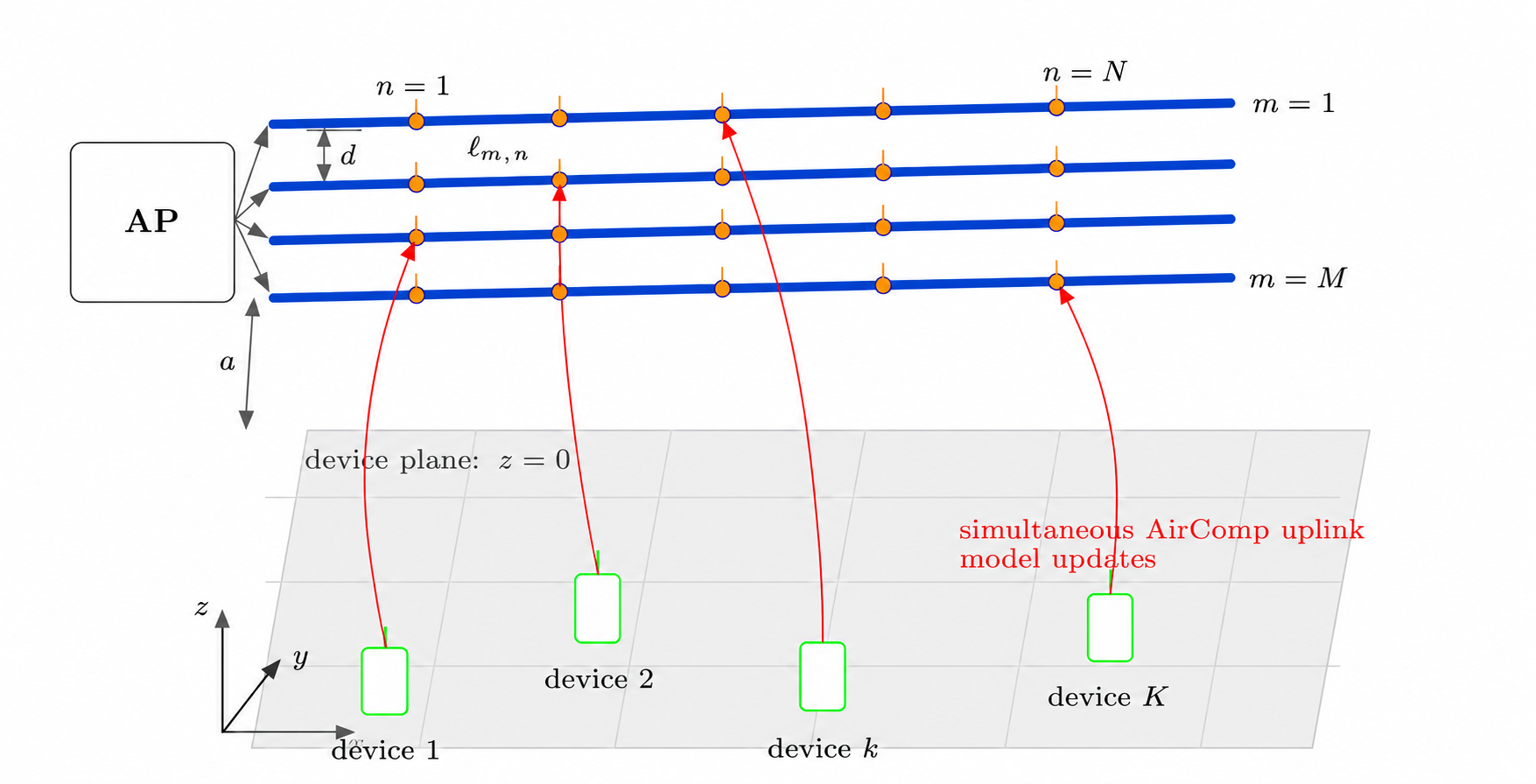
Consider a wireless FL system consisting of an AP and \(K\) single-antenna edge devices indexed by the set \(\mathcal{K}=\{1,\ldots,K\}\), as shown in Fig. 1. Device \(k\in\mathcal{K}\) possesses a local dataset \(\mathcal{D}_k\) with cardinality \(|\mathcal{D}_k|\). The objective of FL is to collaboratively train a global model parameterized by \(\mathbf{w}\) by minimizing the empirical risk \[F(\mathbf{w})=\sum_{k=1}^{K}\frac{|\mathcal{D}_k|}{D}F_k(\mathbf{w}),\] where \(F_k(\mathbf{w})\) denotes the local loss function of device \(k\), and \(D=\sum_{k=1}^{K}|\mathcal{D}_k|\).
Training proceeds over communication rounds following the FedAvg protocol [1]. At each round, the AP broadcasts the current global model to all devices. Each device performs \(J\) local training steps based on its dataset and computes a local update. A subset of devices then simultaneously transmits their updates to the AP for AirComp-based aggregation.
2.1 MIMO PASS Architecture↩︎
The AP is equipped with a multi-input multi-output pinching antenna system (MIMO PASS) consisting of \(M\) dielectric waveguides. Each waveguide is connected to one RF chain and contains \(N\) movable pinching antennas. Accordingly, the AP provides an effective \(M\)-dimensional receive interface.
The \(m\)th waveguide is placed parallel to the \(x\)-axis at lateral coordinate \((m-1)d\) and height \(a\), where \(d\) denotes the spacing between adjacent waveguides. Let \(\ell_{m,n}\) denote the position of the \(n\)th pinching antenna on waveguide \(m\) measured along the waveguide axis. The three-dimensional coordinate of the \(n\)th pinching antenna on waveguide \(m\) is given by \[\mathbf{v}_{m,n}=[\ell_{m,n},(m-1)d,a]^T,\] where \(m\in\{1,\ldots,M\}\) and \(n\in\{1,\ldots,N\}\).
The coordinate of device \(k\) is denoted by \[\mathbf{u}_k=[x_k,y_k,0]^T.\]
Define the pinching position vector on waveguide \(m\) as \[\boldsymbol{\ell}_m=[\ell_{m,1},\ldots,\ell_{m,N}]^T,\] and collect all pinching locations as \[\mathbf{L}=[\boldsymbol{\ell}_1^T,\ldots,\boldsymbol{\ell}_M^T]^T.\]
The pinching positions must satisfy the physical constraints \[\begin{align} 0 \le \ell_{m,1}, \quad &\forall m,\\ \ell_{m,n+1}-\ell_{m,n}\ge \Delta \ell, \quad &\forall m,\; n=1,\ldots,N-1,\\ \ell_{m,N}\le L_m, \quad &\forall m, \end{align}\] where \(L_m\) denotes the length of waveguide \(m\), and \(\Delta \ell\) denotes the minimum allowable spacing between adjacent pinching antennas on the same waveguide, avoiding mutual coupling.
2.2 Uplink Channel Model↩︎
The propagation distance between device \(k\) and the \(n\)th pinching antenna on waveguide \(m\) is \[\begin{align} & D_{k,m}(\ell_{m,n})= \|\mathbf{u}_k-\mathbf{v}_{m,n}\| = \nonumber\\& \sqrt{(x_k-\ell_{m,n})^2+(y_k-(m-1)d)^2+a^2}. \end{align}\]
Following the MIMO PASS uplink channel model, the effective channel coefficient between device \(k\) and waveguide \(m\) is [24] \[g_{k,m}(\boldsymbol{\ell}_m) = \xi \gamma_k \sum_{n=1}^{N} \frac{ e^{-j\kappa\left(D_{k,m}(\ell_{m,n})+i_{\mathrm{ref}}\ell_{m,n}\right)} }{ \sqrt{N}D_{k,m}(\ell_{m,n}) },\] where \(\xi\) is a constant related to the free-space propagation attenuation, \(\gamma_k\in\mathbb{R}_+\) denotes the large-scale channel gain coefficient of device \(k\), \(\kappa=2\pi/\lambda\) is the wave number, \(\lambda\) is the carrier wavelength, and \(i_{\mathrm{ref}}\) denotes the refractive index of the dielectric waveguide.
The effective channel vector between device \(k\) and the AP is defined as \[\mathbf{g}_k(\mathbf{L}) = [g_{k,1}(\boldsymbol{\ell}_1),\ldots,g_{k,M}(\boldsymbol{\ell}_M)]^T \in \mathbb{C}^{M\times1}.\]
Stacking all device channels yields the channel matrix \[\mathbf{G}(\mathbf{L}) = [\mathbf{g}_1(\mathbf{L}),\ldots,\mathbf{g}_K(\mathbf{L})] \in \mathbb{C}^{M\times K}.\]
2.3 AirComp-Based Model Aggregation↩︎
At each communication round, only a subset of devices participates in the uplink transmission. Let \(\mathcal{S}\subseteq\mathcal{K}\) denote the selected device set.
Each selected device \(k\in\mathcal{S}\) transmits a scaled version of its normalized local update \(s_k\)2 as \(\tilde{x}_k=b_k s_k\), where \(b_k\) is the transmit scaling coefficient subject to the power constraint \(|b_k|^2\le P_0\).
The received signal at the AP is \[\mathbf{r} = \sum_{k\in\mathcal{S}}\mathbf{g}_k(\mathbf{L})b_k s_k + \mathbf{n},\] where \(\mathbf{n}\sim\mathcal{CN}(\mathbf{0},\sigma^2\mathbf{I}_M)\) denotes the additive white Gaussian noise vector.
To recover the desired unnormalized aggregate, the AP applies a receive beamforming vector \(\mathbf{m}\in\mathbb{C}^{M}\) and a denoising factor \(\eta>0\), yielding \[\hat{s}= \frac{1}{\sqrt{\eta}}\mathbf{m}^H\mathbf{r}.\]
In FL, the desired aggregation function is the weighted sum \[s= \sum_{k\in\mathcal{S}}\phi_k s_k,\] where \(\phi_k={|\mathcal{D}_k|}\).3
The AirComp aggregation distortion is measured by the mean-square error (MSE) \[\mathrm{MSE}= \mathbb{E}\left[|\hat{s}-s|^2\right].\]
Assuming \(\mathbb{E}[s_k]=0\), \(\mathbb{E}[|s_k|^2]=1\), and \(s_k\) are uncorrelated, the MSE can be expressed as \[\label{eq:mse95expanded} \mathrm{MSE} = \sum_{k\in\mathcal{S}} \left| \frac{1}{\sqrt{\eta}}\mathbf{m}^H\mathbf{g}_k(\mathbf{L})b_k-\phi_k \right|^2 + \frac{\sigma^2\|\mathbf{m}\|^2}{\eta}.\tag{1}\]
3 Optimization Problem Formulation↩︎
The objective of the proposed PASS-enabled AirFL system is to maximize the number of selected devices while ensuring that the aggregation MSE remains below a prescribed threshold. This formulation is a direct consequence of convergence analysis in AirFL systems [2] and has been widely adopted in the literature [6]–[8], [13], [15]. At the communication-design level, this criterion requires channel information and aggregation weights, but does not require instantaneous gradients, losses, or class-distribution information. It therefore provides a practical model-agnostic scheduling surrogate for AirFL, while the final learning performance can still depend on the data partition and on the selected devices.
To this end, the AP jointly designs the device selection set \(\mathcal{S}\), the transmit scaling coefficients \(\{b_k\}\), the receive beamforming vector \(\mathbf{m}\), the denoising factor \(\eta\), and the pinching locations \(\mathbf{L}\). The joint design problem is formulated as \[\label{problem95main} \begin{align} \max_{\mathcal{S},\{b_k\},\mathbf{m},\eta,\mathbf{L}} \quad & |\mathcal{S}| \\ \text{s.t.}\quad & \mathrm{MSE}\le \varepsilon, \\ & |b_k|^2\le P_0,\quad \forall k\in\mathcal{S}, \\ & 0 \le \ell_{m,1}, \quad \forall m, \\ & \ell_{m,n+1}-\ell_{m,n}\ge \Delta \ell,\quad \forall m,\; n=1,\ldots,N-1, \\ & \ell_{m,N}\le L_m,\quad \forall m. \end{align}\tag{2}\]
For any \(k\in\mathcal{S}\) with \(\mathbf{m}^H\mathbf{g}_k(\mathbf{L})\neq 0\), the transmit scaling coefficient that eliminates the first summation term in 1 , i.e., the deterministic alignment error, takes the form [6] \[b_k = \sqrt{\eta}\phi_k \frac{(\mathbf{m}^H\mathbf{g}_k(\mathbf{L}))^H}{|\mathbf{m}^H\mathbf{g}_k(\mathbf{L})|^2}, \qquad k\in\mathcal{S}.\] Indeed, substituting this \(b_k\) sets each effective noiseless aggregation coefficient to \(\phi_k\), so the deterministic alignment error vanishes. The remaining distortion is therefore purely noise-induced and decreases monotonically with \(\eta\). Hence, the optimal denoising factor is the largest one that satisfies the per-device power constraints.
Substituting the above expression into the transmit power constraint yields [6] \[\eta \le \frac{P_0|\mathbf{m}^H\mathbf{g}_k(\mathbf{L})|^2}{\phi_k^2}, \qquad \forall k\in\mathcal{S}.\]
To satisfy all power constraints simultaneously, the denoising factor \(\eta\) must satisfy [6] \[\eta \le \min_{k\in\mathcal{S}} \frac{P_0|\mathbf{m}^H\mathbf{g}_k(\mathbf{L})|^2}{\phi_k^2}.\]
Choosing \(\eta\) as the maximum feasible value minimizes the aggregation MSE. Consequently, the minimum achievable MSE becomes \[\mathrm{MSE} = \frac{\sigma^2}{P_0} \max_{k\in\mathcal{S}} \frac{\phi_k^2\|\mathbf{m}\|^2}{|\mathbf{m}^H\mathbf{g}_k(\mathbf{L})|^2}.\]
Therefore, the aggregation-MSE constraint \(\mathrm{MSE}\le\varepsilon\) is equivalent to \[\max_{k\in\mathcal{S}} \frac{\phi_k^2\|\mathbf{m}\|^2}{|\mathbf{m}^H\mathbf{g}_k(\mathbf{L})|^2} \le \frac{P_0\varepsilon}{\sigma^2}.\]
Define \[\Gamma=\frac{P_0\varepsilon}{\sigma^2}.\]
Then the joint device selection, receive beamforming, and PASS configuration problem can be reformulated as \[\label{problem95reformulated} \begin{align} \max_{\mathcal{S},\mathbf{m},\mathbf{L}} \quad & |\mathcal{S}| \\ \text{s.t.}\quad & \frac{\phi_k^2\|\mathbf{m}\|^2}{|\mathbf{m}^H\mathbf{g}_k(\mathbf{L})|^2} \le \Gamma, \quad \forall k\in\mathcal{S}, \\ & 0 \le \ell_{m,1}, \quad \forall m, \\ & \ell_{m,n+1}-\ell_{m,n}\ge \Delta \ell, \quad \forall m,\; n=1,\ldots,N-1, \\ & \ell_{m,N}\le L_m,\quad \forall m. \end{align}\tag{3}\]
Problem 3 is a nonconvex and combinatorial optimization problem. In the next two sections, we develop the AirPASS alternating optimization framework to solve 3 .
4 Device Selection and Receive Beamforming for Fixed PASS Configuration↩︎
In this section, we study the joint device-selection and receive-beamforming subproblem for a fixed PASS configuration \(\mathbf{L}\). For given \(\mathbf{L}\), the effective uplink channel vectors \(\{\mathbf{g}_k(\mathbf{L})\}_{k\in\mathcal{K}}\) are known. The problem is \[\label{problem95fixedL} \begin{align} \max_{\mathcal{S},\mathbf{m}}\quad & |\mathcal{S}| \\ \text{s.t.}\quad & \frac{\phi_k^2\|\mathbf{m}\|^2}{|\mathbf{m}^H\mathbf{g}_k(\mathbf{L})|^2} \le \Gamma, \qquad \forall k\in\mathcal{S} . \end{align}\tag{4}\]
Problem 4 aims to select as many devices as possible while satisfying the aggregation-MSE requirement. Devices with larger aggregation weights \(\phi_k\) or weaker effective channels \(\mathbf{g}_k(\mathbf{L})\) are harder to schedule, since they require larger effective receive gains. The primary challenge in solving 4 stems from its combinatorial objective coupled with nonconvex quadratic feasibility constraints.
4.1 Problem Reformulation and Main Idea↩︎
The feasibility condition in 4 is homogeneous in \(\mathbf{m}\). Hence, we impose \[\|\mathbf{m}\|^2 = 1\] without loss of optimality. Define \[\mathbf{Q}_k(\mathbf{L}) = \frac{\Gamma}{\phi_k^2}\mathbf{g}_k(\mathbf{L})\mathbf{g}_k^H(\mathbf{L}), \qquad \mathbf{Q}_k(\mathbf{L})\succeq 0 .\] Then device \(k\) is feasible if \[\mathbf{m}^H\mathbf{Q}_k(\mathbf{L})\mathbf{m} \ge 1 .\]
Accordingly, 4 can be rewritten as \[\label{problem95sphere} \begin{align} \max_{\mathbf{m}}\quad & \sum_{k=1}^{K} \mathbb{1}\!\left( \mathbf{m}^H\mathbf{Q}_k(\mathbf{L})\mathbf{m} \ge 1 \right) \\ \text{s.t.}\quad & \|\mathbf{m}\|^2 = 1 . \end{align}\tag{5}\]
Problem 5 is a maximum-cardinality quadratic feasibility problem on the complex unit sphere. This reformulation is a central step of the proposed method: it transforms the original mixed discrete–continuous problem into a sphere-constrained cardinality formulation, making the beamformer geometry explicit while isolating the combinatorial difficulty in the counting objective.
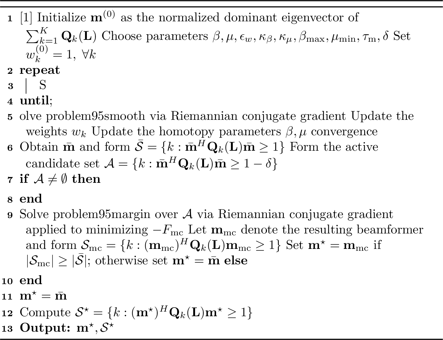
Based on 5 , we develop a homotopy-Riemannian margin-consolidation (HRMC) algorithm for device selection and receive beamforming under fixed PASS configuration. The key idea is to perform both the cardinality-oriented search and the final robustness-oriented consolidation directly on the complex sphere. Thus, the fixed-configuration block remains in the original beamforming space and avoids the lifted matrix variables required by SDR-DC-type methods.
4.2 Smooth Cardinality Approximation↩︎
The main obstacle in 5 is the discontinuous indicator function. To handle it, we introduce a smooth surrogate that approximates the number of violated constraints.
Define the feasibility score \[z_k(\mathbf{m};\mathbf{L}) = \mathbf{m}^H\mathbf{Q}_k(\mathbf{L})\mathbf{m} ,\] and the one-sided violation measure \[v_k(\mathbf{m})=\max\{1-z_k(\mathbf{m};\mathbf{L}),0\}.\] Since the hinge operator is not differentiable, we replace it by the softplus approximation \[\tilde{v}_k(\mathbf{m}) = \frac{1}{\beta}\log\!\left( 1+\exp\!\big(\beta(1-z_k(\mathbf{m};\mathbf{L}))\big) \right),\] where \(\beta>0\) controls the sharpness. To mimic the counting behavior of the cardinality objective, we further introduce the saturating penalty \[\rho_\mu(t)=1-\exp(-t/\mu),\] where \(\mu>0\) is a smoothing parameter.
This leads to the surrogate problem \[\label{problem95smooth} \begin{align} \min_{\mathbf{m}}\quad & F_{\beta,\mu}(\mathbf{m}) = \sum_{k=1}^{K} w_k\,\rho_\mu(\tilde{v}_k(\mathbf{m})) \\ \text{s.t.}\quad & \|\mathbf{m}\|^2=1, \end{align}\tag{6}\] where \(w_k>0\) is the reweighting coefficient associated with device \(k\). This surrogate is one of the key components of the proposed method. It replaces the discontinuous counting objective by a differentiable function while still preserving the selection structure of the original problem: small violations, large violations, and feasible devices are treated differently. The reweighting scheme assigns larger emphasis to devices with smaller surrogate violations, thereby biasing the optimization toward recovering marginal or nearly feasible devices.
4.3 Homotopy-Reweighted Riemannian Optimization↩︎
Problem 6 is naturally defined on the complex sphere \[\mathcal{M}=\{\mathbf{m}\in\mathbb{C}^M:\|\mathbf{m}\|=1\}.\] We solve it directly on \(\mathcal{M}\), which preserves the unit-norm constraint exactly and keeps the dominant optimization in the original beamforming space.
Using the Wirtinger convention for complex-valued variables, the derivative of \(z_k(\mathbf{m};\mathbf{L})\) with respect to \(\mathbf{m}^\ast\) is \[\nabla_{\mathbf{m}^\ast}z_k(\mathbf{m};\mathbf{L}) = \mathbf{Q}_k(\mathbf{L})\mathbf{m} .\] Hence, the Euclidean gradient of 6 is \[\nabla_{\mathbf{m}^\ast}F_{\beta,\mu} = -\sum_{k=1}^{K}\alpha_k\,\mathbf{Q}_k(\mathbf{L})\mathbf{m},\] where \[\alpha_k = w_k\,\rho_\mu'(\tilde{v}_k)\, \frac{1}{1+\exp\!\big(-\beta(1-z_k(\mathbf{m};\mathbf{L}))\big)},\] and \[\rho_\mu'(t)=\frac{1}{\mu}\exp(-t/\mu).\] Projecting onto the tangent space gives the Riemannian gradient \[\mathrm{grad}\,F_{\beta,\mu} = \nabla_{\mathbf{m}^\ast}F_{\beta,\mu} - \mathbf{m}\Re\!\left\{ \mathbf{m}^H\nabla_{\mathbf{m}^\ast}F_{\beta,\mu} \right\}.\]
For initialization, we use the normalized dominant eigenvector of \(\sum_{k=1}^{K}\mathbf{Q}_k(\mathbf{L})\). For fixed \((\beta,\mu)\) and weights \(\{w_k\}\), we solve 6 by the standard Riemannian conjugate-gradient method on \(\mathcal{M}\) [29]. At each iteration, the method constructs a conjugate search direction \(\boldsymbol{\xi}\) in the tangent space of the current point. Given \(\boldsymbol{\xi}\) and a step size \(\tau>0\), the next beamformer is obtained by the normalized retraction \[\mathbf{m}^+ = \mathcal{R}_{\mathbf{m}}(\tau\boldsymbol{\xi}) = \frac{\mathbf{m}+\tau\boldsymbol{\xi}}{\|\mathbf{m}+\tau\boldsymbol{\xi}\|},\] where \(\tau\) is chosen by backtracking line search.
A fixed surrogate pair \((\beta,\mu)\) generally does not provide a good balance between numerical stability and approximation accuracy. We therefore use a homotopy, or continuation, strategy: the algorithm solves a sequence of smooth surrogate problems, each initialized from the previous solution, while gradually sharpening the approximation to the original nonsmooth cardinality objective. In HRMC, this is achieved by increasing the softplus sharpness and decreasing the smoothing level of the saturating violation penalty: \[\beta^{(t+1)}=\min\{\kappa_\beta\beta^{(t)},\beta_{\max}\}, \mu^{(t+1)}=\max\{\mu^{(t)}/\kappa_\mu,\mu_{\min}\}.\] The weights are initialized as \(w_k^{(0)}=1\) and updated as \[\label{eq95weight95update} w_k^{(t+1)} = \frac{1}{\tilde{v}_k(\mathbf{m}^{(t)})+\epsilon_w},\tag{7}\] where \(\mathbf{m}^{(t)}\) denotes the beamformer obtained at homotopy step \(t\). This rule implements the reweighting mechanism introduced in 6 .
After convergence of the homotopy iterations, let \(\bar{\mathbf{m}}\) denote the resulting beamformer and define \[\bar{\mathcal{S}} = \{k:\bar{\mathbf{m}}^H\mathbf{Q}_k(\mathbf{L})\bar{\mathbf{m}}\ge 1\}.\]
4.4 Feasibility-Margin Consolidation↩︎
The homotopy-reweighted stage identifies a beamforming direction that is favorable for device admission. However, some feasible or nearly feasible devices may remain close to the threshold. To improve the robustness of this candidate set, we perform a feasibility-margin consolidation step on the same complex sphere.
Let \(\bar{\mathbf{m}}\) be the beamformer obtained from the homotopy stage, and define \[z_k(\bar{\mathbf{m}};\mathbf{L}) = \bar{\mathbf{m}}^H\mathbf{Q}_k(\mathbf{L})\bar{\mathbf{m}}.\] We form the active candidate set \[\mathcal{A} = \{k:z_k(\bar{\mathbf{m}};\mathbf{L})\ge 1-\delta\},\] where \(\delta>0\) is a small margin parameter. The set \(\mathcal{A}\) contains devices that are already feasible under \(\bar{\mathbf{m}}\), as well as devices within a margin \(\delta\) of feasibility; these are the devices targeted by the local margin-consolidation step.
For \(\mathcal{A}\neq\emptyset\), the weakest active feasibility score is \(\min_{k\in\mathcal{A}}\mathbf{m}^H\mathbf{Q}_k(\mathbf{L})\mathbf{m}\). Since this minimum is nondifferentiable, we replace it with the following smooth soft-min approximation and maximize it: \[\label{problem95margin} \begin{align} \max_{\mathbf{m}}\quad & F_{\mathrm{mc}}(\mathbf{m}) = -\tau_{\mathrm m} \log\!\left( \sum_{k\in\mathcal{A}} \exp\!\left( -\frac{\mathbf{m}^H\mathbf{Q}_k(\mathbf{L})\mathbf{m}}{\tau_{\mathrm m}} \right) \right) \\ \text{s.t.}\quad & \|\mathbf{m}\|^2=1, \end{align}\tag{8}\] where \(\tau_{\mathrm m}>0\) controls the accuracy of the soft-min approximation. As \(\tau_{\mathrm m}\) decreases, \(F_{\mathrm{mc}}(\mathbf{m})\) approaches \(\min_{k\in\mathcal{A}}\mathbf{m}^H\mathbf{Q}_k(\mathbf{L})\mathbf{m}\).
Define \[\pi_k(\mathbf{m}) = \frac{ \exp\!\left( -\mathbf{m}^H\mathbf{Q}_k(\mathbf{L})\mathbf{m}/\tau_{\mathrm m} \right)}{ \sum_{j\in\mathcal{A}} \exp\!\left( -\mathbf{m}^H\mathbf{Q}_j(\mathbf{L})\mathbf{m}/\tau_{\mathrm m} \right)}, \qquad k\in\mathcal{A} .\] The Euclidean gradient of the margin-consolidation objective is \[\nabla_{\mathbf{m}^\ast}F_{\mathrm{mc}}(\mathbf{m}) = \sum_{k\in\mathcal{A}} \pi_k(\mathbf{m})\mathbf{Q}_k(\mathbf{L})\mathbf{m},\] and the corresponding Riemannian gradient is \[\mathrm{grad}\,F_{\mathrm{mc}} = \nabla_{\mathbf{m}^\ast}F_{\mathrm{mc}}(\mathbf{m}) - \mathbf{m}\Re\!\left\{ \mathbf{m}^H\nabla_{\mathbf{m}^\ast}F_{\mathrm{mc}}(\mathbf{m}) \right\}.\] We solve 8 using the same Riemannian conjugate-gradient framework and normalized retraction as in the homotopy stage, applied equivalently to the minimization of \(-F_{\mathrm{mc}}\). If \(\mathcal{A}=\emptyset\), the consolidation step is skipped and \(\mathbf{m}^\star=\bar{\mathbf{m}}\). Otherwise, let \(\mathbf{m}_{\mathrm{mc}}\) denote the beamformer obtained from 8 , and define \(\mathcal{S}_{\mathrm{mc}}=\{k:(\mathbf{m}_{\mathrm{mc}})^H \mathbf{Q}_k(\mathbf{L})\mathbf{m}_{\mathrm{mc}}\ge 1\}\). We set \(\mathbf{m}^\star=\mathbf{m}_{\mathrm{mc}}\) if \(|\mathcal{S}_{\mathrm{mc}}|\ge|\bar{\mathcal{S}}|\), and set \(\mathbf{m}^\star=\bar{\mathbf{m}}\) otherwise.
The final selected set is determined by the original feasibility condition: \[\mathcal{S}^\star = \{k:(\mathbf{m}^\star)^H\mathbf{Q}_k(\mathbf{L})\mathbf{m}^\star\ge 1\}.\]
4.5 Proposed HRMC Algorithm↩︎
Algorithm 2 summarizes the proposed HRMC algorithm for fixed PASS configuration. The method consists of two coordinated stages: homotopy-reweighted Riemannian optimization and active-set feasibility-margin consolidation. The first stage performs the main cardinality-oriented beamformer search, while the second improves the robustness of the active candidate set before the final thresholding decision.
4.6 Complexity Analysis↩︎
The proposed HRMC block has two computational stages.
The first stage solves 6 by homotopy-reweighted Riemannian optimization. In each iteration, the dominant cost is evaluating \(z_k(\mathbf{m};\mathbf{L})\) and \(\mathbf{Q}_k(\mathbf{L})\mathbf{m}\) for all \(k\). Under a dense implementation, this gives \(\mathcal{O}(KM^2)\) per iteration. Since \[\mathbf{Q}_k(\mathbf{L}) = \frac{\Gamma}{\phi_k^2}\mathbf{g}_k(\mathbf{L})\mathbf{g}_k^H(\mathbf{L})\] is rank one, a structure-aware implementation reduces this to \(\mathcal{O}(KM)\).
The second stage solves the margin-consolidation problem 8 . Its per-iteration complexity is \(\mathcal{O}(|\mathcal{A}|M^2)\) under a dense implementation and \(\mathcal{O}(|\mathcal{A}|M)\) when the rank-one structure is exploited. Since \(|\mathcal{A}|\le K\), the per-iteration cost of this stage is upper bounded by that of the first stage.
Therefore, if the homotopy-reweighted stage and the margin-consolidation stage require \(I_1\) and \(I_2\) Riemannian iterations, respectively, a conservative overall bound is \[\mathcal{O}\!\left( I_1KM^2 + I_2|\mathcal{A}|M^2 \right),\] which yields \[\mathcal{O}\!\left( (I_1+I_2)KM^2 \right)\] using \(|\mathcal{A}|\le K\). If the rank-one structure is exploited, the corresponding bound becomes \[\mathcal{O}\!\left( I_1KM + I_2|\mathcal{A}|M \right),\] and hence \[\mathcal{O}\!\left( (I_1+I_2)KM \right).\]
4.7 Discussion↩︎
The fixed-configuration subproblem in 4 has the same essential structure as the learning-oriented AirFL scheduling formulations studied in prior work, namely, maximizing the number of selected devices under an aggregation-MSE requirement. Existing approaches to this class of problems have mainly followed two directions. One direction relies on lifted SDR-DC formulations, where matrix optimization is the main computational tool [6]. Another direction relies on matching-pursuit-type scheduling, which reduces complexity through sequential support updates [8].4
The need for a lightweight yet coupled HRMC block becomes especially important in the proposed alternating framework, where device selection and receive beamforming are updated repeatedly as the PASS configuration changes. In this setting, lifted high-complexity solvers can dominate the overall computational cost, while purely sequential hard-selection rules may produce support updates that are sensitive to intermediate PASS configurations.
The proposed HRMC method takes a different route. For a fixed PASS configuration, the problem is first recast as a sphere-constrained maximum-cardinality quadratic feasibility problem, so that the dominant search is carried out directly in the receive-beamforming space. The subsequent margin-consolidation stage remains on the same manifold and improves the weakest active feasibility scores before the final device-selection decision. Thus, the method avoids the lifted matrix variables used by SDR-DC approaches while retaining a coupled continuous beamformer optimization that is absent from purely greedy scheduling.
| Method | Computational Complexity |
|---|---|
| SDR-DC [6] | \(\mathcal{O}\!\left(K(M^2+K)^3 + K M^6\right)\) |
| HRMC | \(\mathcal{O}\!\left((I_1+I_2)K M^2\right)\) |
| Matching Pursuit [8] | \(\mathcal{O}\!\left(K^2 M^2\right)\) |
The complexity results in Table 1 highlight distinct scaling behaviors. The SDR-DC approach scales cubically in \((M^2+K)\) and includes an additional \(M^6\) term, making it highly sensitive to the receive dimension. Matching pursuit scales quadratically in both \(K\) and \(M\), resulting in lower growth with system size but relying on sequential support decisions. The proposed HRMC method replaces the lifted SDR-DC cost by linear scaling in \(K\) and quadratic scaling in \(M\) under the dense implementation reported in the table, with a reduced \(\mathcal{O}((I_1+I_2)KM)\) implementation possible when the rank-one structure of \(\mathbf{Q}_k(\mathbf{L})\) is exploited. Consequently, HRMC offers a lightweight manifold-based block for device selection and receive beamforming within the proposed alternating PASS-AirFL optimization framework.
5 PASS Antenna Configuration Optimization↩︎
We now address the second block of the AirPASS framework, namely the optimization of the pinching antenna positions assuming that the device set and receive beamformer are fixed. This block is referred to as homotopy-assisted geometry optimization (HAGO). Its role is to reshape the effective uplink channels through antenna placement so as to improve the aggregation feasibility margins of the selected devices.
5.1 PASS Configuration Optimization Problem↩︎
From the aggregation feasibility condition derived earlier, we have \[\frac{\phi_k^2\|\mathbf{m}\|^2}{|\mathbf{m}^H\mathbf{g}_k(\mathbf{L})|^2} \le \Gamma ,\quad \forall k\in\mathcal{S}.\] Since the beamformer is normalized as \(\|\mathbf{m}\|=1\), this condition reduces to \[|\mathbf{m}^H\mathbf{g}_k(\mathbf{L})|^2 \ge \frac{\phi_k^2}{\Gamma},\quad \forall k\in\mathcal{S}.\]
For fixed \((\mathcal{S},\mathbf{m})\), the above inequalities define the PASS-configuration subproblem, namely, determining antenna positions \(\mathbf{L}\) that satisfy the aggregation constraints for all selected devices. Since these constraints are governed by the weakest normalized effective channel among the selected devices, we adopt a max–min refinement that selects a configuration maximizing this quantity: \[\label{prob95pass} \begin{align} \max_{\mathbf{L}} \quad & \min_{k\in\mathcal{S}} \frac{|\mathbf{m}^H\mathbf{g}_k(\mathbf{L})|^2}{\phi_k^2} \\ \text{s.t.}\quad &0\le \ell_{m,1} \le \ell_{m,2}\le \cdots \le \ell_{m,N}\le L_m,\quad \forall m, \\ &\ell_{m,n+1}-\ell_{m,n}\ge \Delta \ell,\quad \forall m,\; n=1,\ldots,N-1 . \end{align}\tag{9}\]
This formulation selects, among admissible antenna configurations, the one that maximizes the worst-user margin and thereby enlarges the feasibility buffer within the selected set.
However, problem 9 is highly nonconvex because the effective channel coefficients depend on antenna positions through nonlinear distance and phase terms. In addition, the minimum operator in the objective is nondifferentiable. The main challenge is therefore to optimize a worst-device-driven configuration criterion under coupled ordering and minimum-spacing constraints on all pinching locations.
5.2 Smooth Approximation of the Worst-Device Objective↩︎
To enable efficient optimization, we replace the minimum operator in 9 with a smooth log-sum-exp approximation. Define \[h_k(\mathbf{L})=|\mathbf{m}^H\mathbf{g}_k(\mathbf{L})|^2 .\] Then introduce the smoothed objective \[f_\tau(\mathbf{L}) = -\tau \log \sum_{k\in\mathcal{S}} \exp \left( -\frac{h_k(\mathbf{L})}{\tau\phi_k^2} \right),\] where \(\tau>0\) is the smoothing parameter. It follows that \[\lim_{\tau\rightarrow 0} f_\tau(\mathbf{L}) = \min_{k\in\mathcal{S}} \frac{h_k(\mathbf{L})}{\phi_k^2}.\] Hence, maximizing \(f_\tau(\mathbf{L})\) provides a smooth approximation of the original worst-device objective.
For large \(\tau\), the surrogate is smoother and easier to optimize, while for small \(\tau\) it becomes a tighter approximation of the minimum operator. This motivates a continuation strategy described next.
5.3 Homotopy Strategy for the Smoothing Parameter↩︎
Following the continuation principle introduced in the HRMC block, HAGO also uses a homotopy schedule for its smoothing parameter. Here, \(\tau\) controls the tradeoff between numerical stability and approximation accuracy. The algorithm starts from a relatively large \(\tau\) and gradually decreases it during the iterations, so that it first explores the PASS configuration under a smooth objective landscape and then progressively focuses on the weakest effective channel.
Specifically, the smoothing parameter is updated as \[\tau^{(t+1)}=\max\{\rho\,\tau^{(t)},\tau_{\min}\}.\]
5.4 Gradient of the Smoothed Objective↩︎
Define \[u_k(\mathbf{L})=\mathbf{m}^H\mathbf{g}_k(\mathbf{L}),\] so that \(h_k(\mathbf{L})=|u_k(\mathbf{L})|^2\). The derivative of \(h_k\) with respect to \(\ell_{m,n}\) is \[\frac{\partial h_k}{\partial\ell_{m,n}} = 2\Re \left\{ u_k^\ast \mathbf{m}^H \frac{\partial\mathbf{g}_k(\mathbf{L})}{\partial\ell_{m,n}} \right\}.\]
Applying the chain rule to the log-sum-exp surrogate yields \[\frac{\partial f_\tau}{\partial\ell_{m,n}} = 2 \sum_{k\in\mathcal{S}} \widetilde{w}_k \Re \left\{ u_k^\ast \mathbf{m}^H \frac{\partial\mathbf{g}_k(\mathbf{L})}{\partial\ell_{m,n}} \right\},\] where \[\widetilde{w}_k = \frac{\exp(-h_k(\mathbf{L})/(\tau\phi_k^2))}{\sum_{j\in\mathcal{S}}\exp(-h_j(\mathbf{L})/(\tau\phi_j^2))} \cdot\frac{1}{\phi_k^2}.\] These weights emphasize devices with weaker normalized effective channels and therefore steer the configuration update toward improving the bottleneck device.
5.5 Derivative of the PASS Channel↩︎
The effective channel coefficient between device \(k\) and waveguide \(m\) is \[g_{k,m}(\boldsymbol{\ell}_m) = \sum_{n=1}^{N} g_{k,m,n},\] where \[g_{k,m,n} = \xi\gamma_k \frac{ e^{-j\kappa(D_{k,m}(\ell_{m,n})+i_{\mathrm{ref}}\ell_{m,n})} }{ \sqrt N\, D_{k,m}(\ell_{m,n}) }.\] The propagation distance is \[D_{k,m}(\ell_{m,n}) = \sqrt{(x_k-\ell_{m,n})^2+(y_k-(m-1)d)^2+a^2}.\] Its derivative is \[\frac{\partial D_{k,m}}{\partial\ell_{m,n}} = \frac{\ell_{m,n}-x_k}{D_{k,m}(\ell_{m,n})}.\]
Therefore, \[\begin{align} &\frac{\partial g_{k,m,n}}{\partial\ell_{m,n}} =\nonumber\\& g_{k,m,n} \Bigg[ -\frac{1}{D_{k,m}(\ell_{m,n})} \frac{\partial D_{k,m}}{\partial\ell_{m,n}} -j\kappa \left( \frac{\partial D_{k,m}}{\partial\ell_{m,n}} +i_{\mathrm{ref}} \right) \Bigg]. \end{align}\]
Since only the \(m\)th waveguide component of \(\mathbf{g}_k(\mathbf{L})\) depends on \(\ell_{m,n}\), we have \[\frac{\partial \mathbf{g}_k(\mathbf{L})}{\partial\ell_{m,n}} = \mathbf{e}_m \frac{\partial g_{k,m,n}}{\partial\ell_{m,n}},\] where \(\mathbf{e}_m\) is the \(m\)th canonical basis vector in \(\mathbb{C}^M\).
5.6 Feasible Reparameterization of Antenna Positions↩︎
Direct optimization over the antenna positions \(\{\ell_{m,n}\}\) is inconvenient because of the ordering and minimum-spacing constraints in 9 . To address this issue, we introduce a reparameterization that guarantees feasibility by construction. This is a key technical step of HAGO, since it converts the constrained configuration design into a smooth unconstrained problem while preserving the joint coupling among all pinching locations.
For each waveguide \(m\), define \(N+1\) unconstrained real variables \(\{u_{m,i}\}_{i=0}^{N}\). We first map them to positive quantities through the softplus function \[r_{m,i}=\log(1+e^{u_{m,i}}), \qquad i=0,1,\ldots,N .\] Let \[T_m=L_m-(N-1)\Delta \ell ,\] which is the remaining allocable length after accounting for the mandatory minimum spacings. A feasible configuration requires \(T_m\ge 0\).
Next, define normalized slack fractions \[q_{m,i}=\frac{r_{m,i}}{\sum_{j=0}^{N} r_{m,j}},\qquad i=0,1,\ldots,N,\] so that \(q_{m,i}>0\) and \(\sum_{i=0}^{N} q_{m,i}=1\).
The antenna positions are then constructed as \[\ell_{m,n} = T_m\sum_{i=0}^{n-1} q_{m,i} + (n-1)\Delta \ell, \qquad n=1,\ldots,N .\]
Under this mapping, the quantities \(T_m q_{m,0}\) and \(T_m q_{m,N}\) represent the left and right endpoint slacks, respectively, while \(T_m q_{m,1},\ldots,T_m q_{m,N-1}\) represent the additional movable gaps between adjacent antennas beyond the mandatory spacing \(\Delta \ell\). Therefore, \[0\le \ell_{m,1}\le \ell_{m,2}\le \cdots \le \ell_{m,N}\le L_m\] and \[\ell_{m,n+1}-\ell_{m,n}\ge \Delta \ell,\qquad n=1,\ldots,N-1,\] hold automatically for every waveguide. Since the softplus mapping gives strictly positive slacks, this reparameterization represents the relative interior of the feasible set; boundary configurations such as \(\ell_{m,1}=0\), \(\ell_{m,N}=L_m\), or \(\ell_{m,n+1}-\ell_{m,n}=\Delta\ell\) can be approached arbitrarily closely as limiting cases. Hence, 9 is converted into an unconstrained optimization over the variables \(\mathbf{U}=\{u_{m,i}\}_{m=1,\ldots,M;\,i=0,\ldots,N}\).
5.7 Geometry Optimization in the Reparameterized Variables↩︎
Using the above mapping, the smoothed objective becomes \(f_\tau(\mathbf{L}(\mathbf{U}))\), which is differentiable with respect to \(\mathbf{U}\). Therefore, the configuration update can be carried out by gradient ascent in the reparameterized variables. By the chain rule, \[\frac{\partial f_\tau}{\partial u_{m,n}} = \sum_{i=1}^{N} \frac{\partial f_\tau}{\partial \ell_{m,i}} \frac{\partial \ell_{m,i}}{\partial u_{m,n}},\] where the derivatives \(\partial f_\tau/\partial \ell_{m,i}\) are obtained from the previous subsection, while \(\partial \ell_{m,i}/\partial u_{m,n}\) follow from the softplus and normalization mapping. Since these terms are smooth, standard backtracking line search can be used to determine the ascent step size.
The update is therefore \[\mathbf{U}^{(t+1)} = \mathbf{U}^{(t)}+\alpha_t \nabla_{\mathbf{U}} f_{\tau^{(t)}}\big(\mathbf{L}(\mathbf{U}^{(t)})\big),\] where \(\alpha_t>0\).
This reparameterized update is an important part of HAGO: it enables joint continuous optimization of all pinching locations while maintaining feasibility at every iteration.
5.8 PASS Configuration Algorithm↩︎
The resulting configuration optimization procedure is summarized in Algorithm 3. The algorithm alternates between computing the gradient of the smoothed worst-device objective with respect to the reparameterized variables and updating the smoothing parameter according to the homotopy rule.
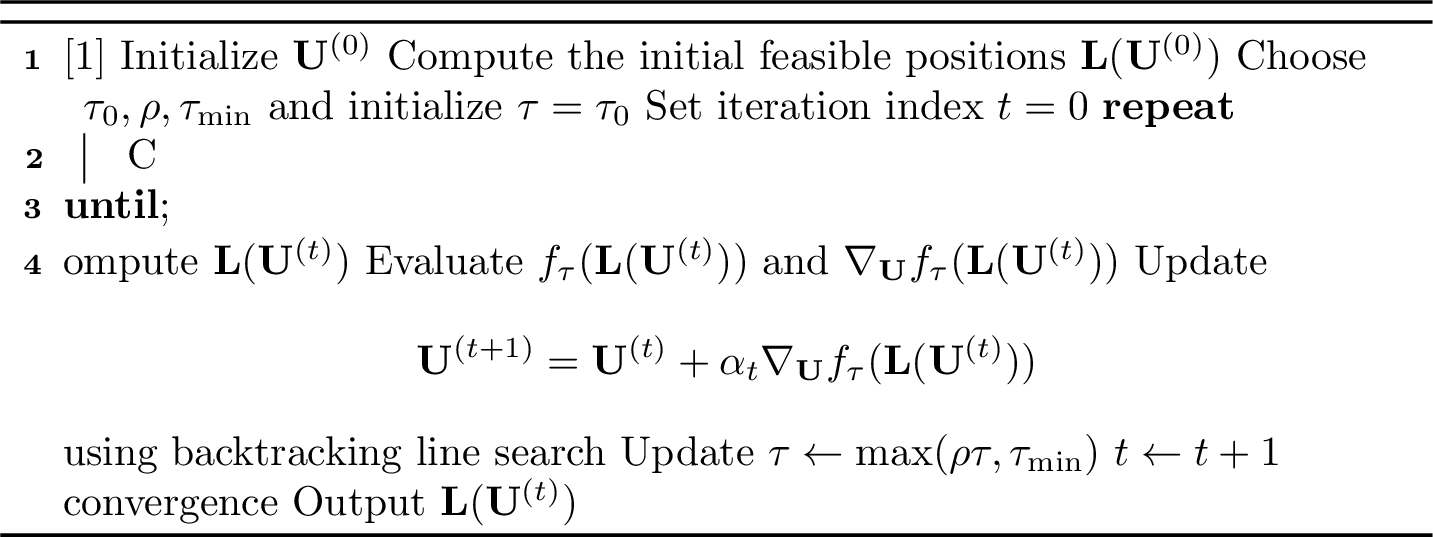
Because the optimization is carried out in the unconstrained variables \(\mathbf{U}\), no explicit projection or post-update repair is required. This is advantageous both algorithmically and analytically, since feasibility of the antenna configuration is guaranteed at every iteration by construction.
Due to the nonconvexity of the configuration design problem, Algorithm 3 converges to a stationary point of the smoothed objective under standard line-search conditions.
5.9 Complexity Analysis↩︎
Let \(|\mathcal{S}|\) denote the number of selected devices. The dominant computational cost of the proposed PASS configuration algorithm comes from evaluating the effective channels and their gradients.
For each selected device \(k\), computing \(\mathbf{g}_k(\mathbf{L})\) requires summing the contributions of all \(MN\) pinching antennas. Likewise, evaluating the derivatives of the smoothed objective requires computing the corresponding partial derivatives with respect to these antenna positions. Therefore, one gradient-evaluation step has complexity \[\mathcal{O}(|\mathcal{S}|MN).\]
The reparameterization from \(\mathbf{U}\) to \(\mathbf{L}(\mathbf{U})\) involves only softplus operations, normalization, and cumulative sums across the \(N\) antennas on each waveguide, and hence has complexity \(\mathcal{O}(MN)\). This term is dominated by the gradient evaluation term above.
Consequently, if the configuration optimization requires \(I_3\) iterations, the total complexity of the PASS-configuration block is \[\mathcal{O} \big( I_3 |\mathcal{S}|MN \big).\]
Thus the antenna-configuration update scales linearly with the number of selected devices, waveguides, and pinching antennas.
5.10 Discussion↩︎
A fundamental characteristic of the PASS configuration problem is that the effective channels arise from coherent superposition along each waveguide, which induces strong coupling among all antenna locations in both amplitude and phase. As a result, the configuration is not naturally separable across individual antenna locations: local adjustments of individual antennas may not lead to predictable local improvements, since each update perturbs the global interference pattern observed by all devices. Existing PASS geometry designs often rely on sequential element-wise updates or grid-based placement searches [24], [26]–[28]. While effective in their respective settings, such strategies can become inefficient when the configuration block must be updated repeatedly within an alternating optimization framework.
The formulation also differs from existing PASS placement problems, which typically optimize communication-centric metrics such as rate or SINR. In contrast, the objective here is governed by a worst-device aggregation constraint induced by AirComp, leading to a bottleneck-driven configuration design rather than a conventional communication-centric placement problem.
The proposed HAGO framework addresses these challenges through coupled first-order geometry optimization with a smooth bottleneck objective and a feasible reparameterization. Thus, all pinching locations are updated jointly while feasibility is maintained by construction.
5.11 AirPASS Alternating Optimization Framework↩︎
The proposed AirPASS method alternates between the two blocks developed above: (i) device selection and receive beamforming for fixed PASS configuration, and (ii) PASS configuration optimization for fixed selected devices and beamformer. The two blocks are tightly coupled: HRMC determines which devices can be aggregated under the current geometry, and HAGO uses that decision to reshape the geometry so that the next device-selection step becomes more favorable. In this way, device selection guides geometry adaptation, and geometry adaptation in turn expands the next selection opportunity.
This alternating procedure is summarized in Algorithm 4.

5.12 Overall Complexity↩︎
Let \(I_{\mathrm{AO}}\) denote the number of outer alternating iterations. Combining the complexity of the two alternating blocks and the final HRMC pass, the overall worst-case complexity is \[\mathcal{O}\!\left( I_{\mathrm{AO}} \left( (I_1+I_2)KM^2+I_3|\mathcal{S}|MN \right) + (I_1+I_2)KM^2 \right),\] where \(I_1\), \(I_2\), and \(I_3\) denote the numbers of iterations in the homotopy-reweighted beamforming optimization, feasibility-margin consolidation, and PASS configuration optimization, respectively, and \(|\mathcal{S}|\) denotes the selected-set size during the geometry-update block, upper bounded by \(K\). Equivalently, this can be written as \(\mathcal{O}\!\left((I_{\mathrm{AO}}+1)(I_1+I_2)KM^2+ I_{\mathrm{AO}}I_3|\mathcal{S}|MN\right)\).
6 Experiments↩︎
In this section, we evaluate the proposed AirPASS framework and compare it against both conventional co-located MIMO baselines and alternative strategies for device selection and receive beamforming.
6.1 Experimental Setup↩︎
We report results on two standard image-classification datasets, namely MNIST and CIFAR-10. For MNIST, we use a lightweight convolutional neural network with two convolutional layers (with 16 and 32 filters, respectively), each followed by max-pooling, and then two fully connected layers with 64 hidden units and a 10-way softmax output. For CIFAR-10, we use a deeper convolutional neural network with three convolutional blocks, each containing two convolutional layers (with 32, 64, and 128 filters, respectively), followed by batch normalization, ReLU activation, max-pooling, and dropout. The network ends with global average pooling, a dense layer with 128 hidden units, and a 10-way softmax output.
The local learning rate is set to \(0.01\) for MNIST and \(0.02\) for CIFAR-10. The batch size is \(32\) for MNIST and \(64\) for CIFAR-10, and \(J = 3\). Each experiment is averaged over \(3\) independent Monte Carlo realizations. The training datasets are partitioned across devices in a non-i.i.d. manner, where each device is randomly assigned samples from three out of the ten classes.
Device locations are independently generated according to the uniform distributions \(x_k\sim\mathcal{U}[4,40]\) m and \(y_k\sim\mathcal{U}[2,10]\) m, while the large-scale fading coefficients are drawn as \(\gamma_k\sim\mathcal{U}[0.8,1.2]\). For the PASS geometry, each waveguide has length \(L_m=40\) m, the spacing between adjacent waveguides is \(d=2\) m, the AP height is \(a=4\) m, and the minimum allowable spacing between adjacent pinching antennas is \(\Delta \ell = 0.95\) m.
For the wireless setup, the transmit power is \(P_0=1\), and the aggregation-MSE threshold is \(\varepsilon=0.03\). The propagation parameters are set to \(\xi=1\), carrier wavelength \(\lambda=0.125\) m, and refractive index \(i_{\mathrm{ref}}=1.45\). The noise variance is determined by the prescribed signal-to-noise ratio (SNR), defined as \(\mathrm{SNR} = \frac{P_0}{\sigma^2}\).
For the optimization blocks, the HRMC subproblem is solved via the proposed homotopy-reweighted Riemannian conjugate-gradient procedure followed by the feasibility-margin consolidation step, both with backtracking line search. The HAGO subproblem is solved via gradient ascent in the reparameterized geometry variables, also with backtracking line search. The initial step sizes are set to \(3\times 10^{-2}\) for HRMC and \(4\times 10^{-2}\) for HAGO.
In the HRMC stage, the homotopy parameters are initialized as \(\beta=10\) and \(\mu=0.08\), and are progressively updated according to the rules in Section IV, with \(\beta\) increasing and \(\mu\) decreasing until reaching \(\beta_{\max}=100\) and \(\mu_{\min}=0.01\). The margin-consolidation stage uses the soft-min parameter \(\tau_{\mathrm m}=0.01\) and active-set threshold \(\delta\).
In the HAGO stage, the smoothing parameter \(\tau\) in the log-sum-exp objective is initialized as \(\tau_0=0.1\) and gradually reduced using the homotopy schedule with \(\rho=0.8\) and \(\tau_{\min}=0.01\).
6.2 Benchmark Schemes↩︎
We consider the following benchmark schemes.
FedAvg: Ideal error-free aggregation, used as an upper bound.
AirPASS: The proposed PASS-enabled AirFL framework with HRMC for device selection and receive beamforming, and HAGO for pinching-antenna geometry optimization.
Co-located MIMO–HRMC (\(M\) and \(M\times N\)): Conventional centralized fixed-array MIMO baselines with either \(M\) receive antennas or \(M\times N\) receive antennas, using the same HRMC block as in AirPASS. The \(M\)-antenna case matches the number of waveguides, whereas the \(M\times N\)-antenna case matches the total number of antenna elements in the PASS receiver. The receive antennas form a uniform linear array with inter-element spacing \(\lambda/2\), centered at the midpoint of the PASS structure, and the PASS channel model in Section II-B is replaced by the corresponding conventional co-located MIMO uplink channel.
AirPASS–SDR-DC: A variant of AirPASS in which the HRMC block is replaced by the SDR-DC method in [6], while the HAGO geometry-optimization block is kept unchanged.
AirPASS–MP: A variant of AirPASS in which the HRMC block is replaced by the matching-pursuit method in [8], while the HAGO geometry-optimization block is kept unchanged.



6.3 AirPASS versus Conventional MIMO Baselines↩︎
Figs. 5 and 6 compare AirPASS with ideal FedAvg and the two conventional fixed-array baselines on MNIST and CIFAR-10, respectively. Several important observations can be made.
First, AirPASS consistently outperforms both conventional MIMO baselines on the two datasets. This confirms that the spatial reconfigurability of PASS creates more favorable effective channels for AirComp-based aggregation than fixed receive arrays. In particular, by jointly optimizing device participation, receive beamforming, and pinching locations, AirPASS is able to admit more devices with reliable aggregation and therefore provide a better learning signal to the global model.
Second, the gain over the baseline with only \(M\) fixed antennas is particularly pronounced, which highlights the importance of the additional spatial degrees of freedom introduced by the multiple pinching antennas on each waveguide. Even when compared with the stronger \(M\times N\) fixed-array baseline, AirPASS still achieves a clear advantage, showing that the gain is not merely due to a larger number of radiating points but also due to their jointly optimized spatial configuration.
Third, the AirPASS curves remain close to the ideal FedAvg benchmark, especially on MNIST. This indicates that the proposed design effectively controls AirComp distortion and preserves most of the statistical benefit of ideal aggregation. The same trend is also visible on CIFAR-10, although the gap to FedAvg becomes slightly larger due to the higher task difficulty and the increased sensitivity of deeper models to aggregation distortion.
6.4 Comparison with Alternative Fixed-Configuration Strategies↩︎
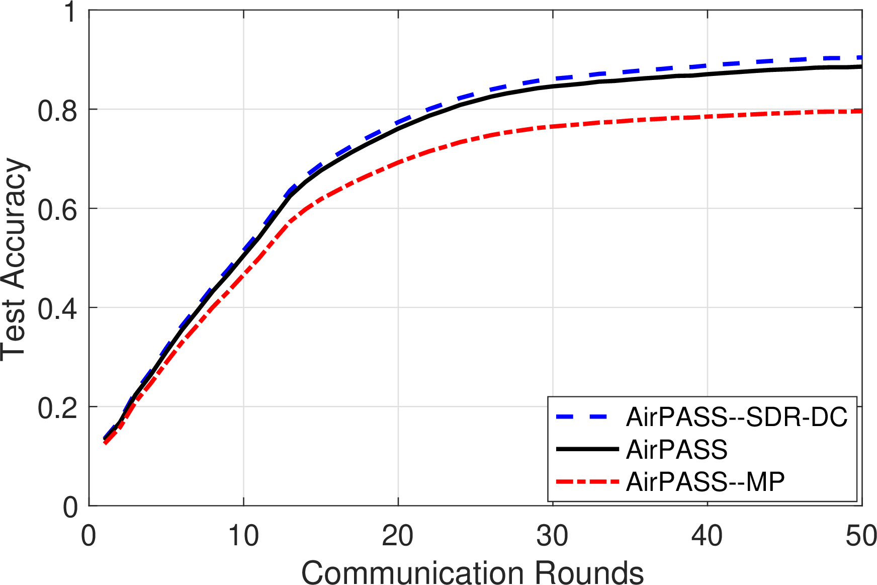
Figs. 7 and 8 compare the proposed AirPASS implementation against two alternative AirPASS-based variants, AirPASS–SDR-DC and AirPASS–MP, in order to isolate the contribution of the HRMC block.
The first observation is that the proposed AirPASS significantly outperforms AirPASS–MP on both datasets. This shows that the smooth manifold-based optimization is much more effective than a purely greedy scheduling strategy for the present maximum-cardinality quadratic-feasibility problem. The improvement is especially relevant in the early and intermediate rounds, where a stronger selected set leads to faster model improvement.
The second observation is that AirPASS remains highly competitive with AirPASS–SDR-DC. From the plots, the SDR-DC variant attains a slightly higher final accuracy in the tested settings, but the gap is small on both MNIST and CIFAR-10. This is an important result because the SDR-DC method operates in a lifted semidefinite domain and is therefore substantially heavier computationally. In contrast, the proposed HRMC block performs both the cardinality-oriented search and the margin-consolidation step directly in the original beamforming space, without lifted matrix variables. Therefore, the results support the claimed complexity–performance tradeoff of HRMC.
6.5 Impact of the Number of Waveguides↩︎
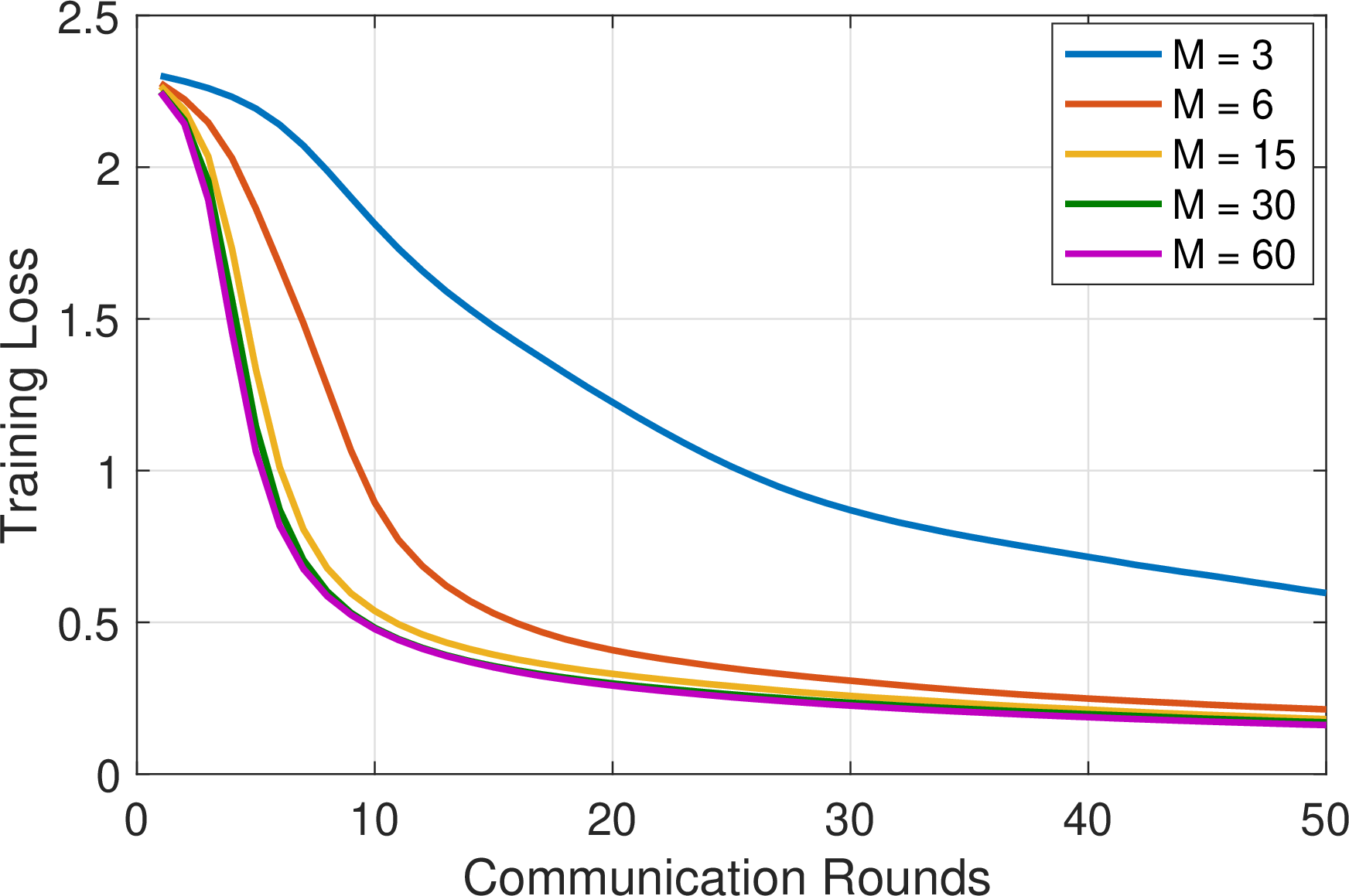
Fig. 9 shows the training loss of AirPASS on MNIST for different numbers of waveguides \(M\). Increasing \(M\) clearly accelerates convergence and reduces the final loss. This behavior is expected because a larger number of waveguides provides more receive dimensions, which improves the flexibility of the beamformer and makes it easier to align the effective user channels for AirComp aggregation.
Another important observation is that the gain exhibits diminishing returns. The improvement from very small \(M\) to moderate \(M\) is substantial, whereas the gap between larger values becomes progressively smaller. This indicates that once the receive beamformer has enough spatial degrees of freedom to serve most users reliably, further increasing \(M\) mainly yields incremental rather than transformative gains.
6.6 Impact of the Number of Pinching Antennas↩︎
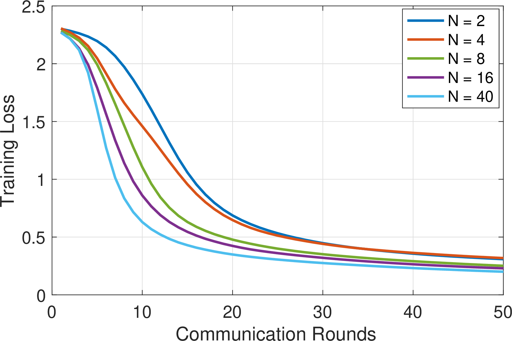
Fig. 10 illustrates the impact of the number of pinching antennas per waveguide, \(N\), on the MNIST training loss. A larger \(N\) consistently improves convergence speed and reduces the loss floor. This confirms that more pinching antennas provide finer spatial shaping capability along each waveguide, which in turn enables the PASS geometry optimizer to create stronger and better-balanced effective channels.
As in the previous experiment, the improvement is most visible when moving from small to moderate values of \(N\), whereas the gain becomes less dramatic for very large values. This suggests that a moderate number of pinching antennas can already capture most of the geometry benefit, while very large \(N\) mainly refines the effective array configuration further.
6.7 Impact of SNR↩︎
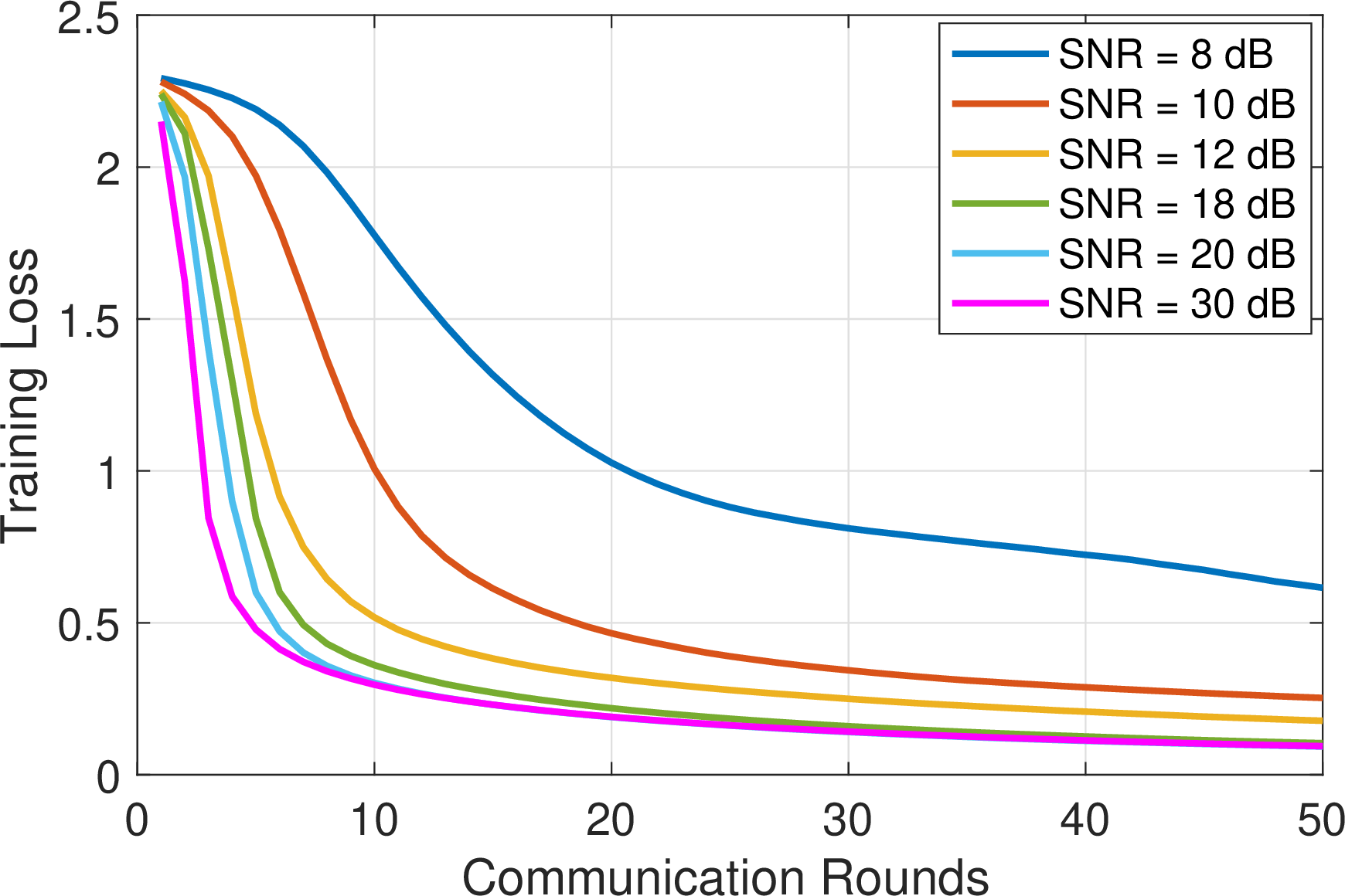
Fig. 11 shows the MNIST training loss for different SNR values. As expected, increasing the SNR improves learning performance substantially. Higher SNR reduces AirComp aggregation distortion, which makes the received global update closer to its ideal value and therefore stabilizes FL convergence.
The figure also shows that the most dramatic improvement occurs in the low-to-moderate SNR regime. Once the SNR becomes sufficiently large, the curves become much closer to each other, indicating that the aggregation quality is no longer dominated by noise alone and that the system has entered a regime where the remaining performance gap is mainly governed by other factors such as finite scheduling feasibility and residual model-side optimization effects.
6.8 Device Selection Performance versus SNR↩︎
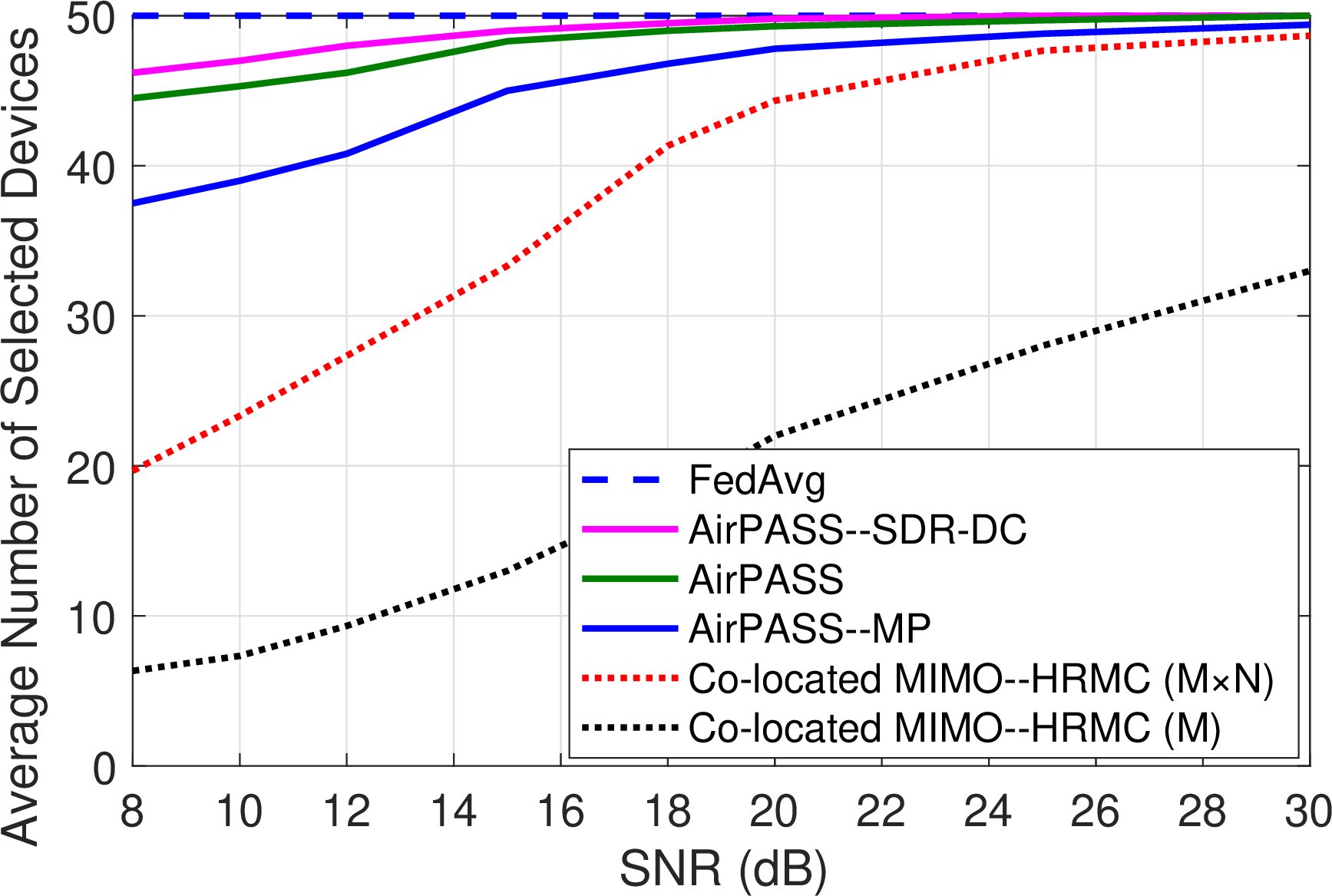
Fig. 12 shows the average number of selected devices versus SNR for AirPASS and different benchmark schemes. AirPASS consistently admits more devices than the conventional co-located MIMO baselines, with a particularly large gain at low SNR. As the SNR increases, AirPASS approaches full participation, closely matching the ideal FedAvg case.
Compared to AirPASS-based variants, AirPASS–SDR-DC provides only marginal improvement, indicating that the proposed method already operates near the optimal feasibility boundary. In contrast, AirPASS–MP selects noticeably fewer devices at low SNR, confirming the limitations of greedy scheduling under stringent constraints. At high SNR, all schemes gradually converge as the feasibility constraints become less restrictive.
7 Conclusion↩︎
This paper studied over-the-air federated learning with pinching antenna systems and proposed AirPASS, a PASS-enabled framework that jointly optimizes device selection, receive beamforming, and pinching-antenna locations under the learning-oriented objective of maximizing the number of participating devices subject to an aggregation-distortion constraint. For the joint device-selection and receive-beamforming block, we developed a homotopy-Riemannian margin-consolidation algorithm that combines smooth cardinality approximation, homotopy-reweighted Riemannian optimization, and active-set feasibility-margin consolidation. For the geometry-design block, we proposed a homotopy-assisted gradient-based PASS optimization method with a feasible reparameterization that enforces antenna ordering and minimum spacing by construction. Simulation results showed that AirPASS increases the number of admissible devices under the aggregation constraint, particularly at low SNR, and translates this gain into improved learning performance over conventional co-located MIMO baselines. At the same time, it remains close to ideal FedAvg and approaches the performance of SDR-DC benchmarks while maintaining a substantially more attractive complexity profile and clearly outperforming matching-pursuit scheduling.
References↩︎
S. M. Azimi-Abarghouyi is with the Department of Electrical Engineering, Chalmers University of Technology, Gothenburg, Sweden (Email: azimimo@chalmers.se). C. G. Brinton is with the School of Electrical and Computer Engineering, Purdue University, West Lafayette, IN USA (Email: cgb@purdue.edu).↩︎
Here, \(s_k\) denotes a scalar entry of the normalized local model update vector. As standard in AirComp-based FL, the same scalar formulation applies element-wise across model coordinates, and the resulting MSE expression characterizes the distortion of each aggregated entry.↩︎
We use the unnormalized weight \(\phi_k=|\mathcal{D}_k|\) in the AirComp design to keep the intermediate feasibility formulation tractable. The standard FedAvg normalization is applied after aggregation by scaling the recovered sum with \(1/\sum_{j\in\mathcal{S}}|\mathcal{D}_j|\).↩︎
It should be emphasized that these prior methods operate under fixed receiver architectures and do not incorporate PASS-related design variables. In contrast, the present work embeds this subproblem within a broader joint optimization that includes PASS configuration.↩︎