A Good Initialization is All You Need for Faithful Visual Attribution
July 07, 2026
Abstract
Faithful visual attribution identifies which image regions support a model prediction. Search-based perturbation methods lead the insertion–deletion faithfulness frontier by masking regions and measuring score changes, but they usually output a complete ordering of all regions. Many applications, especially MLLM attribution and repair, only need a compact top-\(k\) evidence mask. We study this mask-first attribution problem. An exactly \(k\)-region mask is combinatorial: useful evidence can depend on interactions among fine regions. Coarse grouping can stabilize early search but aggregates redundant content, whereas one-step scoring can miss high-value combinations. We introduce two forward-only methods. CoPAIR uses a PhaseWin–Greedy gap diagnosis to construct coarse singleton/pair candidates that warm-start full-ordering search. TRACE directly searches fixed-cardinality fine-region masks with cross-entropy sampling, elite retention, and distribution updates, with a finite-budget recovery analysis. The resulting evidence set can be returned as a compact attribution mask or used to initialize Greedy or PhaseWin when a complete ranking is required. Across ImageNet classification with CLIP ViT-L/14, CLIP RN101, and ResNet-101, our initialized search methods establish a new state-of-the-art frontier for faithful full-ordering attribution under inclusive forward-call accounting. On POPE and RePOPE with Qwen2.5-VL-3B-Instruct and LLaVA-v1.5-7B, TRACE+Greedy gives the strongest search-based MLLM attribution results. Direct TRACE masks further achieve single-point RePOPE repair rates of \(94.44\%\) and \(96.00\%\), showing that compact evidence masks can be actionable attribution outputs, not merely prefixes of full rankings.
1 Introduction↩︎
Faithful visual attribution asks which image regions actually support a model prediction. Because explanations are used as evidence of model reliance, a plausible heatmap is insufficient: faithfulness should be tested by intervening on the image and measuring how the model response changes. Insertion and deletion curves provide this operational test by asking whether selected regions recover the prediction and whether removing them destroys it [1]–[3].
Most strong attribution benchmarks assume a full-ordering contract: a method ranks all image regions so that every prefix can be evaluated by insertion or deletion. This is useful for full-curve evaluation, but many downstream uses only need a compact evidence set. In MLLM hallucination attribution and repair, the practical question is often not how to rank every region, but which small set of visual evidence supports a generated answer or intervention. We therefore treat the fixed-size top-\(k\) evidence mask as a primary attribution object, while retaining compatibility with full-ordering evaluation.
This mask-first contract changes the optimization problem. The best \(k\)-region mask need not be a prefix of a greedy ranking, since its value can depend on interactions among fine regions. One-step scores can miss evidence that is only useful in combination, while coarse grouping can stabilize search but may aggregate redundant content. The challenge is to find a sparse, high-value fine-region evidence set under a black-box, forward-only evaluation budget.
Search-based perturbation is the right foundation for this goal because it evaluates masked inputs and directly optimizes quantities aligned with faithfulness, unlike gradient-based explanations such as Grad-CAM [4] and Integrated Gradients [5]. LIMA [2] showed that Greedy region search gives strong insertion faithfulness, and later work extended this view to object-level foundation models [3] and autoregressive MLLM token generation [6]. However, Greedy costs \(O(n^2)\) forward passes. PhaseWin [7] reduces this cost, but its extended analysis shows that the residual gap to Greedy concentrates on partition-sensitive samples [8]. This suggests that early evidence quality is also a granularity problem: fine regions can fragment evidence that would be more stable at a coarser scale. This diagnosis motivates CoPAIR (Coarse Pairwise Attribution Initializer with Release). CoPAIR clusters fine regions into coarse spatial groups, evaluates strong coarse singletons and pairs, and releases the selected candidate back into fine-region continuation search. It is therefore a principled initializer for Greedy or PhaseWin derived from the PhaseWin–Greedy gap. Its limitation is the same aggregation that makes it useful: a coarse group can merge object parts, background fragments, and redundant fine regions, so it is not a minimal compact explanation. Thus CoPAIR improves full-ordering initialization, but does not solve the mask-first problem.
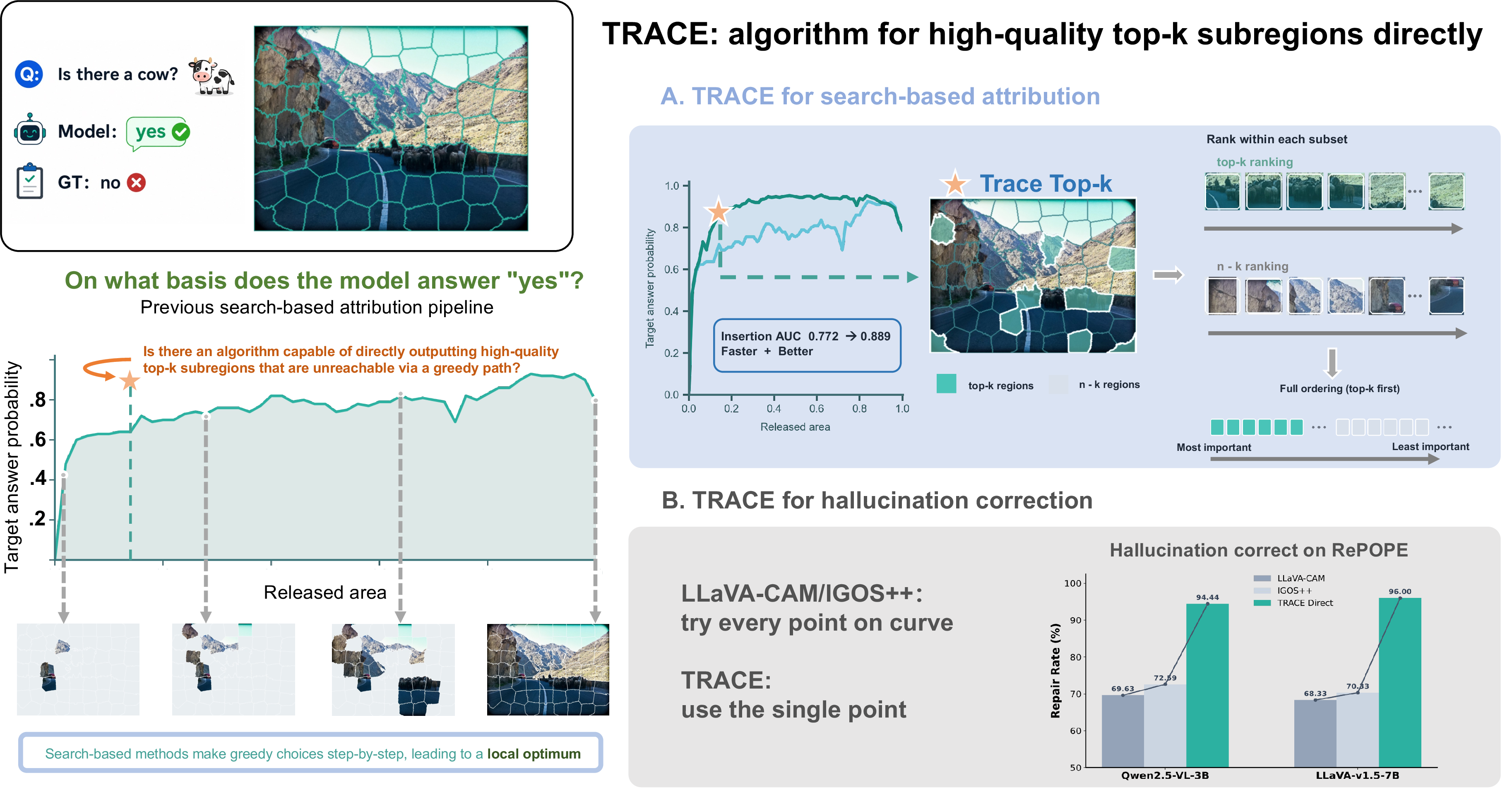
We therefore introduce TRACE (Top-\(k\) Region Attribution via Cross-Entropy), a forward-only method that directly optimizes fixed-cardinality fine-region masks. TRACE samples \(k\)-hot candidate masks, evaluates them by the model response, keeps elite samples, and updates the sampling distribution toward high-scoring evidence combinations. The returned mask can be used directly as the attribution object, or used to initialize Greedy or PhaseWin when a complete ordering is required. We also provide a finite-budget recovery analysis showing how the cross-entropy updates increase probability mass on near-optimal evidence basins. Figure 1 illustrates this shift from stepwise full-curve attribution to an actionable top-\(k\) evidence anchor.
Empirically, CoPAIR and TRACE establish a new state-of-the-art frontier for faithful visual attribution under a black-box, forward-only interface. On ImageNet-derived classification splits with SLICO-64 regions [9], CLIP ViT-L/14, CLIP RN101 [10], and ResNet-101 [11], our initialized search methods improve task-relevant full-ordering faithfulness over raw search under inclusive forward-call accounting. On POPE [12] and RePOPE [13] with Qwen2.5-VL-3B-Instruct [14] and LLaVA-v1.5-7B [15], TRACE+Greedy gives the strongest search-based MLLM attribution results. Direct TRACE masks further repair \(94.44\%\) and \(96.00\%\) of RePOPE cases, respectively, using a single mask intervention rather than a full repair curve.
Our contributions are:
We formulate compact top-\(k\) evidence masks as a primary output contract for faithful visual attribution, while preserving full-ordering evaluation.
We derive CoPAIR from the PhaseWin–Greedy gap diagnosis as a coarse-pair initializer, and address its aggregation limitation with TRACE, a cross-entropy search method for fixed-size fine-region masks.
We establish a new state-of-the-art frontier for forward-only faithful visual attribution across ImageNet classification, POPE, and RePOPE, and show that direct TRACE masks enable effective single-point MLLM repair.
2 Related Work↩︎
2.0.0.1 Visual attribution methods.
Gradient and activation saliency methods [4], [5], [16]–[28] are computationally efficient but require white-box access and do not directly measure the causal relationship between input regions and model outputs, a concern also reflected in saliency sanity checks [29]. Perturbation-based methods [1], [30]–[34] and Shapley-style attribution [35]–[39] evaluate the model on masked inputs and are therefore applicable to any black-box model, but achieve only moderate faithfulness due to their unstructured or approximate nature. Search-based attribution [2], [3] achieves the highest faithfulness by casting region ranking as combinatorial optimization: a greedy algorithm iteratively selects the region with the greatest marginal score gain, producing a provably high-quality ordering at \(O(n^2)\) cost. PhaseWin [7], [8] reduces this to \(O(n)\) via partition-dominant structure, but the remaining gap to Greedy concentrates on partition-sensitive tail cases. Our work targets a complementary object: a compact evidence mask that can be returned directly when no full ranking is needed, or used as the initial state for Greedy and PhaseWin when a complete ordering is required.
2.0.0.2 Attribution tasks.
The dominant benchmark for visual attribution is image classification on ImageNet [40] with CNN, ViT, and CLIP backbones [10], [11], [41], where attribution identifies which image regions drive the classifier’s top-class prediction. Faithful attribution for multimodal large language models (MLLMs) and adjacent vision-language systems such as LLaVA-v1.5-7B [15], [42], BLIP-2 [43], Grounding DINO [44], Florence-2 [45], and Qwen2.5-VL-3B-Instruct [14] is far less explored, despite recent MLLM explanation work [28], [46]–[49]. Because answer generation depends on the interplay of visual tokens and language context, gradient signals through the visual encoder are unreliable proxies for causal influence. Defining the attribution score as the first-token probability of the generated answer makes perturbation-based search directly applicable, but the \(O(n^2)\) cost of Greedy has historically made this impractical at scale. EAGLE [6] adapts greedy search to autoregressive MLLM attribution and introduces hallucination attribution and repair evaluation on POPE and RePOPE [12], [13]. TRACE keeps the same black-box scoring interface while directly searching for a fixed-size visual evidence mask; this mask can either support repair directly or warm start the full search protocol.
3 Method↩︎
3.1 Search-Based Attribution Setup↩︎
We build on the search-based visual attribution framework of Greedy [2], VPS [3], and PhaseWin [7]. The input image is partitioned into fine regions \[U=\{u_1,\ldots,u_n\}.\] For a target \(y\), let \(f_y(x)\in[0,1]\) denote the normalized model response on image \(x\), such as a class probability or an MLLM answer-token probability under a fixed prompt. For any subset \(S\subseteq U\), its retained image is \[x_S = m(S)\odot x + \bigl(1-m(S)\bigr)\odot x_0 , \label{eq:masked-image}\tag{1}\] where \(m(S)\) is the binary mask induced by \(S\) and \(x_0\) is a baseline image. We use the same proxy family as prior faithful attribution search: \[F(S)=\operatorname{Suff}(S) \quad \text{or} \quad F(S)=\alpha \operatorname{Suff}(S) +(1-\alpha)\operatorname{Necc}(S), \label{eq:proxy}\tag{2}\] where \[\operatorname{Suff}(S)=f_y(x_S), \qquad \operatorname{Necc}(S)=1-f_y(x_{U\setminus S}).\]
A full-ordering attribution method returns a permutation \(\Pi=(\pi_1,\ldots,\pi_n)\) of regions, so any prefix \(\{\pi_1,\ldots,\pi_t\}\) can be evaluated by insertion or deletion curves. However, many downstream uses of attribution do not require the whole ordering. They need a compact top-\(k\) evidence mask \(S\) with \(|S|=k\), for example to highlight the visual evidence behind an MLLM token or to perform a single repair intervention. We therefore separate two output contracts: initialization for full-ordering search, and direct fixed-size fine-region mask attribution. Furthermore, the greedy nature of seeking a local optimum at each step—while yielding excellent ranking performance—often results in a loss of the ability to explore the global optimum. If we can directly output a high-value top-k prefix, the attribution performance of search-based algorithms will also be correspondingly enhanced.
Search with initialization framework. Given an initialized fine-region prefix \[\Pi_0=(\pi_1,\ldots,\pi_r), \qquad S_{\mathrm{init}}=\{\pi_1,\ldots,\pi_r\},\] a continuation algorithm \(\mathcal{A}\) completes the remaining ordering as \[\Pi_{\mathrm{tail}} = \mathcal{A}\bigl(F; S_{\mathrm{init}}, U\setminus S_{\mathrm{init}}\bigr), \qquad \Pi=\Pi_0\oplus \Pi_{\mathrm{tail}} . \label{eq:initialized-search}\tag{3}\] Regions not included in \(S_{\mathrm{init}}\) are released back to the live pool and can be selected later by the continuation search.
3.1.0.1 Internal ordering and release.
For any candidate set \(C\subseteq U\), we order its fine regions by greedy marginal rescoring inside \(C\): \[\pi_t = \arg\max_{u\in C\setminus P_{t-1}} F(P_{t-1}\cup\{u\}), \qquad P_{t-1}=\{\pi_1,\ldots,\pi_{t-1}\}. \label{eq:internal-greedy}\tag{4}\] Given a partial-release ratio \(\gamma\in(0,1]\), we keep the shortest prefix satisfying \[r = \min\left\{ t: F(P_t)\ge \gamma F(C) \right\}, \qquad S_{\mathrm{init}}=P_r. \label{eq:release-rule}\tag{5}\] The remaining regions \(C\setminus S_{\mathrm{init}}\) are released to \(U\setminus S_{\mathrm{init}}\) before downstream search.
3.2 CoPAIR: Coarse Pairwise Attribution Initializer with Release↩︎
We derive our initial design strategy by contrasting the PhaseWin algorithm with the greedy approach. As detailed in [8], the greedy method’s apparent advantage in handling the long tail can be reinterpreted as repeated early-prefix recovery: when an unfavorable fine partition fragments visual evidence, global rescoring lets the model recover decisive fragments as the context evolves. Coarser partitions aggregate these fragments into more stable attribution units, mitigating this tail behavior directly. This observation motivates CoPAIR (Algorithm 2), a deterministic coarse-spatial initializer that evaluates coarse singleton and pair candidates first, then integrates the selected evidence into the fine-region continuation search.
Let \(\mathcal{G}=\{G_1,\ldots,G_c\}\) denote a deterministic centroid-based coarse partition of the fine regions, \[G_i\subseteq U,\quad G_i\cap G_j=\emptyset\;(i\ne j), \qquad \bigcup_{i=1}^c G_i=U, \label{eq:coarse-partition}\tag{6}\] with coarse count \[c = \operatorname{clip} \bigl(\operatorname{round}(\beta\sqrt{|U|}),c_{\min},c_{\max}\bigr). \label{eq:copair-count}\tag{7}\]
CoPAIR’s working assumption is that, once local evidence has been absorbed within coarse groups, the early cross-group value is dominated by singleton and pairwise terms. Formally, for \(I\subseteq[c]\), \[F\Bigl(\bigcup_{i\in I}G_i\Bigr) = \phi_\emptyset +\sum_{i\in I}\phi_i +\sum_{\substack{i<j\\i,j\in I}}\phi_{ij} +\sum_{\substack{J\subseteq I\\ |J|\ge 3}}\phi_J, \label{eq:coarse-interactions}\tag{8}\] where the higher-order remainder \(\sum_{|J|\ge 3}\phi_J\) is assumed small for the early coarse candidates the initializer considers. Pair enumeration is therefore not an independent scoring heuristic but an explicit search over coarse-level interactions.
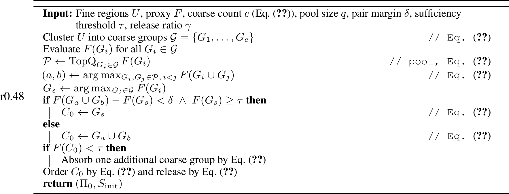
CoPAIR evaluates every coarse singleton and retains the top-\(q\) candidates as a high-sufficiency pool, \[\mathcal{P} = \operatorname{TopQ}_{G_i\in\mathcal{G}} F(G_i), \label{eq:copair-pool}\tag{9}\] then exhaustively searches pairs within that pool, \[(a,b) = \arg\max_{G_i,G_j\in\mathcal{P},\, i<j} F(G_i\cup G_j). \label{eq:copair-pair}\tag{10}\] Writing \(G_s=\arg\max_{G_i\in\mathcal{G}}F(G_i)\), \(C_{\mathrm{pair}}=G_a\cup G_b\), and \(\Delta=F(C_{\mathrm{pair}})-F(G_s)\), the pair-gain margin \(\delta\) and sufficiency threshold \(\tau\) select the initial coarse candidate \[C_0 = \begin{cases} G_s, & \Delta < \delta \;\land\;F(G_s)\ge\tau,\\ C_{\mathrm{pair}}, & \text{otherwise}. \end{cases} \label{eq:copair-fallback}\tag{11}\]
If \(F(C_0)<\tau\), CoPAIR absorbs one additional coarse group by greedy sufficiency improvement, \[\begin{align} G_h = \arg\max_{G\in\mathcal{P}:\,G\cap C_0=\emptyset} F(C_0\cup G), \\ C_0 \leftarrow C_0\cup G_h . \end{align} \label{eq:copair-third-block}\tag{12}\] applied at most once regardless of whether \(C_0\) initially holds one group (\(G_s\)) or two (\(C_{\mathrm{pair}}\)), so the candidate never exceeds three coarse groups.
Finally, CoPAIR applies the internal greedy ordering and release rules defined in Eqs. 4 –5 to \(C_0\), yielding \((\Pi_0, S_{\mathrm{init}})\) as a starting point for continuation search — the return step of Algorithm 2. CoPAIR thus serves as a structured initializer for both Greedy and PhaseWin. Notably, it is not intended to solve the fixed-\(k\) fine-region mask problem directly; that objective requires stepping outside this specific search framework, a task the core TRACE algorithm described below addresses directly.
3.3 TRACE: Top-k Region Attribution via Cross-Entropy↩︎
TRACE (Algorithm 3) directly targets the fixed-cardinality fine-region mask problem. A candidate mask is represented by \[\begin{align} z\in\{0,1\}^{|U|}, \; \|z\|_0=k, \; S(z)=\{u_i:z_i=1\}. \label{eq:trace-mask} \end{align}\tag{13}\]
Unlike CoPAIR, which constructs a coarse candidate for continuation search, TRACE searches the exactly-\(k\) fine-region mask space directly. The returned mask is the best candidate observed under the finite forward budget, not a certified global optimum; Appendix 6 gives the finite-budget recovery analysis and the notation used for this probabilistic view.
TRACE adapts the cross-entropy method [50] to the discrete \(k\)-hot space: it maintains logits \(\theta\in\mathbb{R}^{|U|}\), samples candidate masks, retains elite candidates, and updates the distribution toward regions that repeatedly appear in high-scoring masks.
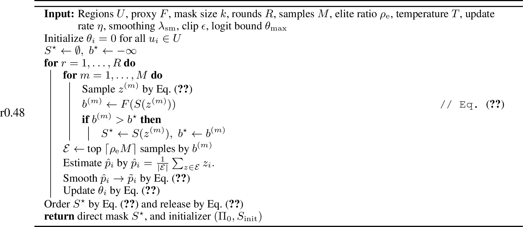
At round \(r\), each candidate is sampled by Gumbel-top-\(k\) perturbation [51]: for sample \(m\), draw \(g_i^{(m)}\sim\operatorname{Gumbel}(0,1)\) i.i.d.and select \[{!}{ \begin{align} z_i^{(m)} = \mathbf{1}\left[ i\in \operatorname{TopK} \left\{ \theta_j/T+g_j^{(m)} \right\}_{j=1}^{|U|} \right], \label{eq:trace-sampling} \end{align} }\tag{14}\] where \(T\) is the temperature. The candidate score is \[b^{(m)} = F(S(z^{(m)})). \label{eq:trace-score}\tag{15}\] Let \(\mathcal{E}\) be the top \(\lceil\rho_{\mathrm e}M\rceil\) samples by \(b^{(m)}\), where \(\rho_{\mathrm e}\) is the elite ratio. The empirical elite inclusion frequency is \(\hat{p}_i = \frac{1}{|\mathcal{E}|} \sum_{z\in\mathcal{E}} z_i .\)
Exact maximum-likelihood fitting of a Gumbel-top-\(k\) distribution to elite sets has no closed-form componentwise update, so TRACE instead uses an inclusion-moment surrogate: the smoothed marginal target \[\tilde{p}_i = (1-\lambda_{\mathrm{sm}})\hat{p}_i +\lambda_{\mathrm{sm}}\frac{k}{|U|}, \label{eq:trace-smooth}\tag{16}\] drives the logit update \[\theta_i \leftarrow \operatorname{clip} \left( (1-\eta)\theta_i + \eta\operatorname{logit} \bigl(\operatorname{clip}(\tilde{p}_i,\epsilon,1-\epsilon)\bigr), -\theta_{\max},\theta_{\max} \right), \label{eq:trace-update}\tag{17}\] where \(\eta\) is the update rate, \(\epsilon\) prevents saturated logits, and \(\theta_{\max}\) bounds the logits.
As shown in Algorithm 3, TRACE tracks the best observed mask incrementally as each candidate is scored, equivalently \(S^\star = \arg\max_{S(z)\;\text{evaluated}} F(S(z)).\) When the task only needs a compact evidence set, \(S^\star\) is returned directly as the final attribution mask. When a complete ordering is required, TRACE applies the same internal greedy ordering and release rule from Eqs. 4 –5 to \(S^\star\), obtaining \((\Pi_0,S_{\mathrm{init}})\), and then uses the continuation interface in Eq. 3 .
The nominal TRACE search evaluates \(RM\) candidate masks before duplicate caching. Under the sufficiency-only proxy used in the main experiments, each uncached candidate requires one model forward, and masks from the same round can be evaluated as a batch. If the combined sufficiency–necessity proxy in Eq. 2 is used instead, each uncached candidate requires both the retained and complement evaluations. The default TRACE budget is thus independent of the number of fine regions once \(R\), \(M\), and \(k\) are fixed, while the continuation cost depends on the remaining live pool.
4 Experiments↩︎
We evaluate two attribution contracts. When a complete ordering is required, TRACE and CoPAIR initialize Greedy (G) or PhaseWin (PW) and are evaluated by insertion–deletion replay. When only a compact evidence set is required, the selected mask is applied directly as a single repair intervention. All tables report task-matched metrics and, for forward-only methods, inclusive selection cost. All initializer hyperparameters, including CoPAIR coarse-pair settings, TRACE sampling settings, duplicate caching, internal greedy ordering, and the \(0.8\) partial-release rule, are reported in Appendix 8.1. Additional protocol details and table conventions are given in Appendix 8.
4.1 Setup and Baselines↩︎
For image classification, we follow the faithful visual attribution protocol used by LIMA, VPS, and PhaseWin [2], [3], [7]. We evaluate CLIP ViT-L/14 and CLIP RN101 [10], and supervised ResNet-101 [11], on ImageNet-derived Correct, Cause, and Repair splits [40] with SLICO-64 regions [9]. The non-search classification baselines include RISE [1], HSIC [34], vanilla gradient saliency [16], Grad-ECLIP [25], IG2 [5], and IGOS++ [49]. For MLLMs, we evaluate the POPE decision-faithfulness and RePOPE repair settings [12], [13] with Qwen2.5-VL-3B-Instruct [14] and LLaVA-v1.5-7B [15]. The MLLM attribution and repair protocol follows EAGLE [6]; its non-search references include LLaVA-CAM [48] and IGOS++ [49].
4.2 Metrics and Accounting↩︎
All scores use normalized target responses \(f_y(x)\in[0,1]\). For ordered attribution, we report insertion AUC (Ins; higher is better), deletion AUC (Del; lower is better), the insertion score at 50% released area (50?), and the maximum insertion score (High). Correct, Cause, and POPE emphasize Ins; classification Repair and RePOPE emphasize High. For single-point RePOPE repair, direct masks are evaluated by Repair Rate, with Correct/Total and Failed reporting the corresponding counts. Full ordered repair metrics such as AMCR, CSR@10, and CorrectionRate are deferred to Appendix 8. MEC(k) reports thousands of selection-time model forwards and excludes insertion/deletion replay. For initialized rows, MEC is inclusive: it includes uncached initializer calls and downstream continuation calls. Under the default sufficiency-only TRACE scoring, each uncached sampled mask uses one forward; using the combined sufficiency–necessity proxy would require both retained and complement evaluations. MEC is compared only within the forward-only family and is left blank for gradient, CAM, and forward-backward optimization methods.
4.3 Image Classification Attribution↩︎
| Method | Correct | Cause | Repair | ||||||||||||||||||||||||||||||||||||||||||
|---|---|---|---|---|---|---|---|---|---|---|---|---|---|---|---|---|---|---|---|---|---|---|---|---|---|---|---|---|---|---|---|---|---|---|---|---|---|---|---|---|---|---|---|---|---|
| 2-6(lr)7-11(l)12-16 | Del | @50 | High | MEC(k) | Del | @50 | High | MEC(k) | Ins | Del | @50 | MEC(k) | |||||||||||||||||||||||||||||||||
| RISE | 0.6173 | 0.3103 | 0.8110 | 0.9325 | 2.00 | 0.4019 | 0.1484 | 0.5769 | 0.7551 | 2.00 | 0.1986 | 0.0458 | 0.3786 | 0.4555 | 2.00 | ||||||||||||||||||||||||||||||
| HSIC | 0.6624 | 0.2617 | 0.8398 | 0.9223 | 0.50 | 0.3806 | 0.1481 | 0.5752 | 0.7078 | 0.50 | 0.1369 | 0.0593 | 0.3286 | 0.3614 | 0.50 | ||||||||||||||||||||||||||||||
| Gradient | 0.4353 | 0.4750 | 0.5148 | 0.9118 | – | 0.2555 | 0.2740 | 0.3253 | 0.6889 | – | 0.0964 | 0.0924 | 0.1874 | 0.3172 | – | ||||||||||||||||||||||||||||||
| Grad-ECLIP | 0.6420 | 0.2802 | 0.8067 | 0.9309 | – | 0.3811 | 0.1603 | 0.5560 | 0.7264 | – | 0.1818 | 0.0492 | 0.4117 | 0.4609 | – | ||||||||||||||||||||||||||||||
| IG2 | 0.4083 | 0.4971 | 0.4610 | 0.9119 | – | 0.2415 | 0.2836 | 0.2956 | 0.6892 | – | 0.0915 | 0.1007 | 0.1739 | 0.3157 | – | ||||||||||||||||||||||||||||||
| IGOS++ | 0.5018 | 0.3992 | 0.6265 | 0.9136 | – | 0.2740 | 0.2247 | 0.3678 | 0.6878 | – | 0.1114 | 0.0836 | 0.2229 | 0.3291 | – | ||||||||||||||||||||||||||||||
| Greedy (G) | 0.8431 | 0.1173 | 0.9597 | 0.9787 | 4.08 | 0.7237 | 0.0500 | 0.8853 | 0.9131 | 4.09 | 0.5448 | 0.0197 | 0.7749 | 0.8009 | 4.09 | ||||||||||||||||||||||||||||||
| PhaseWin (PW) | 0.8037 | 0.1510 | 0.9308 | 0.9707 | 1.73 | 0.6604 | 0.0563 | 0.8325 | 0.8953 | 2.00 | 0.4482 | 0.0206 | 0.6696 | 0.7298 | 2.00 | ||||||||||||||||||||||||||||||
| CoPAIR+PW | \(0.8419^{+.0382}\) | 0.1617 | 0.9588 | 0.9736 | \(1.47_{-.26}\) | \(0.7034^{+.0430}\) | 0.0745 | 0.8717 | 0.9013 | \(1.79_{-.21}\) | 0.5152 | 0.0248 | 0.7688 | \(0.7867^{+.0569}\) | \(2.04_{+.03}\) | ||||||||||||||||||||||||||||||
| TRACE+PW | \(0.8451^{+.0414}\) | 0.1631 | 0.9551 | 0.9736 | \(1.52_{-.20}\) | \(0.7193^{+.0589}\) | 0.0747 | 0.8821 | 0.9076 | \(1.83_{-.17}\) | 0.5241 | 0.0265 | 0.7757 | \(0.7961^{+.0663}\) | \(2.06_{+.06}\) | ||||||||||||||||||||||||||||||
| CoPAIR+G | \(0.8625^{+.0194}\) | 0.1344 | 0.9692 | 0.9796 | \(3.60_{-.48}\) | \(0.7370^{+.0133}\) | 0.0680 | 0.8925 | 0.9132 | \(3.52_{-.57}\) | 0.5545 | 0.0226 | 0.7947 | \(0.8105^{+.0096}\) | \(3.60_{-.49}\) | ||||||||||||||||||||||||||||||
| TRACE+G | 0.1342 | 0.9677 | 0.9799 | \(3.69_{-.39}\) | 0.0676 | 0.9003 | 0.9226 | \(3.63_{-.46}\) | 0.5632 | 0.0236 | 0.8007 | \(3.65_{-.44}\) | |||||||||||||||||||||||||||||||||
2.1pt

Table 1 gives the full CLIP ViT-L/14 landscape, including perturbation, gradient, optimization-based, and search-based methods. Superscripts on initialized rows report the absolute gain over the corresponding raw search in the emphasized metric; MEC subscripts report the cost change against the same raw search. The search family is already much stronger than non-search baselines, but initialization still moves the frontier. TRACE+G gives the best task-relevant score in all three splits: Correct Ins improves from 0.8431 to 0.8679, Cause Ins from 0.7237 to 0.7527, and Repair High from 0.8009 to 0.8190. These gains are not obtained by spending more search: the inclusive MEC for TRACE+G is lower than raw Greedy in each split. PW-based continuation also benefits from initialization, although its inclusive MEC can increase slightly on Repair when the seed cost is not fully offset by the smaller continuation problem. Figure 4 shows representative Correct-split cases behind Table 1: the initialized curve recovers the class score earlier, and the displayed masks concentrate the early evidence on the object regions that support the prediction.
Table 2 checks whether the pattern depends on the CLIP ViT-L/14 backbone. We only show the search family here, and defer the full baseline landscape for CLIP RN101 and ResNet-101 to Appendix 9.3. The result is useful precisely because it is not a single-method sweep. On CLIP RN101, CoPAIR+G is the strongest variant for the emphasized metrics, suggesting that coarse spatial pairing can be valuable when the backbone favors coarser evidence units. On ResNet-101, TRACE+G is strongest on Correct Ins, Cause Ins, and Repair High. Across both backbones, at least one initialized search variant improves the emphasized metric over its raw continuation baseline, showing that initialization changes the attribution search frontier rather than merely reformatting the same ranking.
Furthermore, we conducted ablation studies on \(k\) and various hyperparameters of TRACE using classification scenarios. We also performed comparative experiments to demonstrate the necessity of the probabilistic mask. These experimental results validate the robustness of TRACE. Detailed experimental results are provided in Appendix 9.
| Method | Correct | Cause | Repair | ||||||||||||||||||||||||||||||||||||||||||
|---|---|---|---|---|---|---|---|---|---|---|---|---|---|---|---|---|---|---|---|---|---|---|---|---|---|---|---|---|---|---|---|---|---|---|---|---|---|---|---|---|---|---|---|---|---|
| 2-6(lr)7-11(l)12-16 | Del | @50 | High | MEC(k) | Del | @50 | High | MEC(k) | Ins | Del | @50 | MEC(k) | |||||||||||||||||||||||||||||||||
| Greedy (G) | 0.6677 | 0.0462 | 0.8243 | 0.9134 | 4.08 | 0.5163 | 0.0223 | 0.6655 | 0.7780 | 4.08 | 0.3195 | 0.0092 | 0.4739 | 0.5478 | 4.08 | ||||||||||||||||||||||||||||||
| PhaseWin (PW) | 0.5691 | 0.0500 | 0.6725 | 0.8886 | 1.79 | 0.4087 | 0.0230 | 0.4947 | 0.7366 | 1.83 | 0.2265 | 0.0090 | 0.3012 | 0.4657 | 1.52 | ||||||||||||||||||||||||||||||
| CoPAIR+PW | \(0.6688^{+.0997}\) | 0.0783 | 0.8128 | 0.8975 | \(1.67_{-.12}\) | \(0.5019^{+.0932}\) | 0.0378 | 0.6483 | 0.7505 | \(1.90_{+.08}\) | 0.2983 | 0.0122 | 0.4633 | \(0.5170^{+.0513}\) | \(1.87_{+.35}\) | ||||||||||||||||||||||||||||||
| TRACE+PW | \(0.6376^{+.0685}\) | 0.0750 | 0.7618 | 0.8928 | \(1.76_{-.03}\) | \(0.4753^{+.0666}\) | 0.0377 | 0.6000 | 0.7437 | \(1.92_{+.09}\) | 0.2908 | 0.0117 | 0.4246 | \(0.5073^{+.0416}\) | \(1.82_{+.30}\) | ||||||||||||||||||||||||||||||
| CoPAIR+G | 0.0746 | 0.8535 | 0.9134 | \(3.39_{-.68}\) | 0.0360 | 0.7031 | 0.7824 | \(3.39_{-.70}\) | 0.3348 | 0.0119 | 0.5084 | \(3.43_{-.65}\) | |||||||||||||||||||||||||||||||||
| TRACE+G | \(0.6852^{+.0175}\) | 0.0718 | 0.8262 | 0.9102 | \(3.58_{-.50}\) | \(0.5260^{+.0097}\) | 0.0373 | 0.6725 | 0.7708 | \(3.56_{-.52}\) | 0.3344 | 0.0116 | 0.4913 | \(0.5563^{+.0085}\) | \(3.64_{-.44}\) | ||||||||||||||||||||||||||||||
| Greedy (G) | 0.8407 | 0.1301 | 0.9554 | 0.9605 | 4.08 | 0.7390 | 0.0479 | 0.8958 | 0.9155 | 4.09 | 0.5482 | 0.0173 | 0.7604 | 0.7758 | 4.09 | ||||||||||||||||||||||||||||||
| PhaseWin (PW) | 0.8043 | 0.1483 | 0.9344 | 0.9462 | 1.75 | 0.6802 | 0.0536 | 0.8450 | 0.8883 | 1.87 | 0.4670 | 0.0185 | 0.6705 | 0.7067 | 1.80 | ||||||||||||||||||||||||||||||
| CoPAIR+PW | \(0.8145^{+.0102}\) | 0.1630 | 0.9402 | 0.9469 | \(1.49_{-.26}\) | \(0.6971^{+.0169}\) | 0.0659 | 0.8665 | 0.8901 | \(1.67_{-.20}\) | 0.5017 | 0.0214 | 0.7341 | \(0.7479^{+.0412}\) | \(1.87_{+.07}\) | ||||||||||||||||||||||||||||||
| TRACE+PW | \(0.8214^{+.0171}\) | 0.1581 | 0.9414 | 0.9487 | \(1.52_{-.22}\) | \(0.7035^{+.0233}\) | 0.0648 | 0.8603 | 0.8916 | \(1.69_{-.18}\) | 0.5120 | 0.0214 | 0.7358 | \(0.7511^{+.0444}\) | \(1.86_{+.06}\) | ||||||||||||||||||||||||||||||
| CoPAIR+G | \(0.8394^{-.0013}\) | 0.1451 | 0.9551 | 0.9602 | \(3.65_{-.43}\) | \(0.7346^{-.0044}\) | 0.0606 | 0.8971 | 0.9142 | \(3.57_{-.51}\) | 0.5377 | 0.0206 | 0.7662 | \(0.7778^{+.0020}\) | \(3.63_{-.45}\) | ||||||||||||||||||||||||||||||
| TRACE+G | 0.1420 | 0.9559 | 0.9616 | \(3.73_{-.35}\) | 0.0597 | 0.8892 | 0.9139 | \(3.64_{-.44}\) | 0.5490 | 0.0201 | 0.7671 | \(3.65_{-.44}\) | |||||||||||||||||||||||||||||||||
1.8pt
4.4 MLLM Hallucination Attribution↩︎
Table 3 keeps the full MLLM attribution landscape in the main text, because hallucination attribution is the setting where compact evidence masks are most directly actionable. The table groups results by model and dataset. LLaVA-CAM and IGOS++ provide useful non-search references, but they are far below search-based methods on insertion faithfulness. On POPE, TRACE+G gives the best Ins for both Qwen2.5-VL-3B and LLaVA-v1.5-7B. On RePOPE, raw Greedy remains competitive in Ins for Qwen, but the repair-relevant High metric is highest for TRACE+G on both models. This distinction matters: RePOPE asks whether the selected evidence can recover the corrected answer, so the peak confidence along the insertion trajectory is the more direct signal for repair.
| Dataset | Method | Qwen2.5-VL-3B | LLaVA-v1.5-7B | ||||||
|---|---|---|---|---|---|---|---|---|---|
| 3-6(l)7-10 | Del | MEC(k) | Del | MEC(k) | |||||
| POPE | LLaVA-CAM | 0.7652 | 0.7736 | 0.9506 | – | 0.7563 | 0.7735 | 0.9270 | – |
| IGOS++ | 0.7754 | 0.7542 | 0.9504 | – | 0.7879 | 0.7594 | 0.9277 | – | |
| Greedy (G) | 0.9305 | 0.3707 | 0.9750 | 4.15 | 0.9152 | 0.4841 | 0.9484 | 4.25 | |
| PhaseWin (PW) | 0.9253 | 0.4159 | 0.9735 | 2.24 | 0.9090 | 0.5254 | 0.9466 | 1.54 | |
| RePOPE | LLaVA-CAM | 0.3745 | 0.3919 | 0.6873 | – | 0.3697 | 0.3628 | 0.6737 | – |
| IGOS++ | 0.3721 | 0.3874 | 0.6916 | – | 0.3592 | 0.3784 | 0.6815 | – | |
| Greedy (G) | 0.8055 | 0.1284 | 0.9245 | 4.09 | 0.7683 | 0.1603 | 0.8982 | 4.24 | |
| PhaseWin (PW) | 0.7783 | 0.1424 | 0.9122 | 2.06 | 0.7487 | 0.1719 | 0.8893 | 1.71 | |
3.2pt
4.5 Direct Evidence Masks for RePOPE Repair↩︎
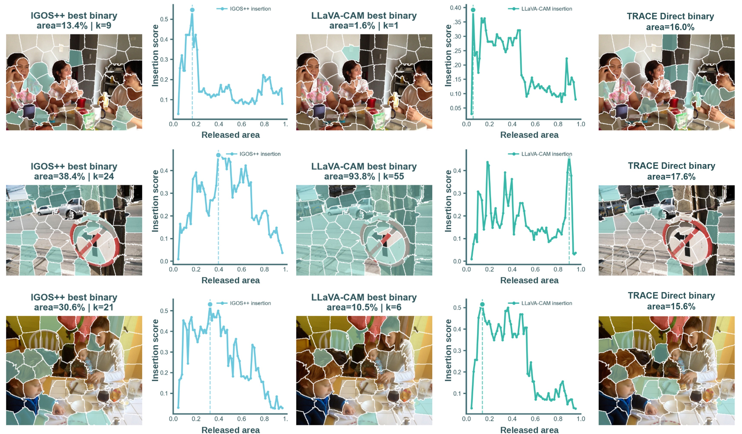
The previous tables evaluate ordered insertion curves. Table 4 tests the mask-first use case directly: a single selected evidence mask is applied as one repair intervention on RePOPE. This setting does not require ranking every region. Direct TRACE masks repair 94.44% of Qwen cases and 96.00% of LLaVA cases, substantially above the LLaVA-CAM and IGOS++ full-curve repair rates. CoPAIR Direct is also stronger than these non-search baselines, but the gap between CoPAIR and TRACE is large, matching our method design: coarse pairing is a useful initializer, whereas direct fine-region mask search is the more appropriate tool when the output itself is a compact evidence mask. The full ordered repair protocol, including CSR@10, is reported in Appendix 9.6; the memory-saving deployment used for the parenthesized engineered memory numbers in Table 4 is detailed in Appendix 8.4. Figure 5 visualizes representative cases where full-curve LLaVA-CAM and IGOS++ do not find a repairing prefix, while TRACE Direct returns a compact mask that repairs the model answer.
| Model | Method | Protocol | Mem. (GB) | Time (s) | |||
|---|---|---|---|---|---|---|---|
| Qwen2.5-VL-3B | LLaVA-CAM | full curve | 69.63 | 188/270 | 82 | 27.1 (16.0) | 11.3 |
| IGOS++ | full curve | 72.59 | 196/270 | 74 | 35.2 (18.4) | 22.0 | |
| LLaVA-v1.5-7B | LLaVA-CAM | full curve | 68.33 | 205/300 | 95 | 37.1 (16.3) | 15.4 |
| IGOS++ | full curve | 70.33 | 211/300 | 89 | 93.9 (18.9) | 22.5 | |
3.4pt
5 Conclusion↩︎
We presented TRACE, a forward-only method for faithful top-\(k\) visual attribution. It directly searches fixed-size fine-region evidence masks and delivers two operating modes: a standalone binary-mask mode for tasks that require only a compact evidence set, and an initialization mode that improves full-ordering Greedy or PhaseWin search. CoPAIR provides a complementary deterministic initializer based on coarse spatial grouping and pairwise evidence enumeration, but the central contribution is the TRACE mask: it handles non-geometric fine-region combinations, can support repair directly, and reduces redundant early search when a complete ranking is required. Both are model-agnostic and validated on image classification (ImageNet-1K, SLICO-64; CLIP ViT-L/14, CLIP RN101, ResNet-101), MLLM decision-faithfulness attribution on POPE, and repair-oriented evidence recovery on RePOPE (Qwen2.5-VL-3B-Instruct and LLaVA-v1.5-7B).
5.0.0.1 Limitations.
The initialization overhead (\(c^2\) for CoPAIR or \(RM\) for TRACE) is negligible for large \(n\) but may dominate when \(n\) is small. TRACE’s stochastic sampling introduces run-to-run variance, which is small in practice but non-zero. The fixed-\(k\) constraint in TRACE requires choosing mask size \(k\) in advance.
6 Additional TRACE Notes↩︎
Section 3.3 gives the TRACE objective, Gumbel-top-\(k\) sampling rule, elite update, and continuation interface. This appendix avoids restating those equations and records only the implementation-level conventions and scope limitations that are useful when interpreting the experiments.
6.1 Candidate Masks and Returned Objects↩︎
TRACE samples only fixed-cardinality fine-region masks. Every evaluated candidate therefore contains exactly \(k\) distinct regions, and no rejection step or post-hoc cardinality repair is needed. In the implementation, a candidate mask is identified by the sorted set of selected region indices. This representation is used for duplicate detection and for storing the best observed candidate during the cross-entropy rounds.
The returned mask is empirical rather than certified: it is the highest-scoring candidate observed under the allocated model-evaluation budget. This distinction matters because the proxy \(F(S)\) is a black-box, nonconvex set objective induced by masked model responses. We therefore do not claim that TRACE solves the global optimum over all \(\binom{n}{k}\) masks; the method is a budgeted search procedure that concentrates samples around regions repeatedly appearing in elite fixed-size masks.
When the downstream task is mask-oriented, this best observed set is returned directly as the attribution or repair mask. When the downstream task requires a full ordering, the same set is used as the initialized prefix described in Eq. 3 . Thus the direct-mask and full-ordering uses share one searched object, rather than using separate attribution procedures.
6.2 Why Not Independent Region Scores?↩︎
A one-step score for each region is cheaper, but it does not model the interaction among selected regions. In visual attribution, this interaction is common: two object parts may be redundant, a background fragment may only matter together with an object region, and an MLLM answer token may depend on a specific combination of local visual cues. Independent scores also do not enforce the output contract that many downstream uses require: a compact mask of exactly \(k\) regions.
Independent Bernoulli sampling has the opposite issue. It can model uncertainty over regions, but the sampled cardinality varies unless an extra constraint or projection is introduced. TRACE uses Gumbel-top-\(k\) sampling because the sampled object is already feasible for the target mask family. This keeps the optimization distribution, the evaluated candidates, and the final output in the same fixed-cardinality space.
6.3 Budget and Caching Scope↩︎
The nominal TRACE budget is \(RM\) candidate masks for \(R\) rounds and \(M\) samples per round. Duplicate masks can occur, especially after the sampling distribution becomes concentrated. In that case, the implementation reuses the stored score instead of issuing another model call. The MEC values reported for initialized rows are inclusive: they include the initializer calls that survive caching and the subsequent continuation calls made by Greedy or PhaseWin.
This accounting is deliberately narrower than wall-clock runtime. MEC is a forward-call count for comparable forward-only selection procedures; it does not attempt to price backward passes, optimizer steps, KV-cache memory, or hardware placement. Those runtime and memory details are reported separately where they matter, especially for the MLLM repair comparison in Table 4.
6.4 Probabilistic Recovery Under a Phase-Structured Attribution Model↩︎
We next record a finite-budget recovery bound for TRACE. The structural assumptions used in this subsection are not new modeling claims of this paper. They are inherited from the extended PhaseWin analysis [8], which interprets the hard tail of search-based visual attribution through partition-sensitive semantic evidence blocks. This inheritance includes the block-level monotonicity assumption used below: adding activated semantic evidence blocks should not decrease the dominant attribution value. We use the same phase-structured view only to make explicit when the cross-entropy updates in TRACE can improve over non-adaptive random search.
Let \(U=\{u_1,\ldots,u_n\}\) be the fine-region set and let \[\mathcal{C}_k(U)=\{S\subseteq U: |S|=k\}\] be the feasible family of exactly-\(k\) masks. For a nonnegative attribution proxy \(F:2^U\to\mathbb{R}_+\), define the fixed-\(k\) optimum and the best TRACE value observed under a budget of \(R\) rounds and \(M_{\mathrm{samp}}\) masks per round as \[\mathrm{opt} = \max_{S\in\mathcal{C}_k(U)}F(S), \qquad \mathrm{opt}_{\mathrm{trace}} = \max_{\substack{0\le r\le R-1\\1\le j\le M_{\mathrm{samp}}}} F(S_{r,j}), \label{eq:app-trace-opt-values}\tag{18}\] where \(\mathrm{opt}>0\). We write \(M_{\mathrm{samp}}\) in this subsection to avoid confusing the per-round sample count with the optimum value; it is the same quantity denoted by \(M\) in Algorithm 3. For an approximation ratio \(\mu\in(0,1)\), define the near-optimal mask set \[\mathcal{G}_\mu = \{S\in\mathcal{C}_k(U): F(S)\ge \mu\,\mathrm{opt}\}. \label{eq:app-trace-near-optimal-set}\tag{19}\] Then \(\mathrm{opt}_{\mathrm{trace}}/\mathrm{opt}\ge \mu\) holds exactly when at least one evaluated mask lies in \(\mathcal{G}_\mu\).
Let \(Q_{\theta_r}\) be the Gumbel-top-\(k\) sampling distribution used by TRACE in round \(r\), and define \[p_r^\mu = Q_{\theta_r}(\mathcal{G}_\mu). \label{eq:app-trace-round-hit-prob}\tag{20}\] Conditioned on the round-\(r\) sampling distribution, the probability that all \(M_{\mathrm{samp}}\) masks miss \(\mathcal{G}_\mu\) is \((1-p_r^\mu)^{M_{\mathrm{samp}}}\). Therefore, \[\Pr\left[ \frac{\mathrm{opt}_{\mathrm{trace}}}{\mathrm{opt}} \ge \mu \right] \ge 1- \prod_{r=0}^{R-1}(1-p_r^\mu)^{M_{\mathrm{samp}}}. \label{eq:app-trace-generic-hit-bound}\tag{21}\] This identity is correct but hides the attribution geometry inside \(p_r^\mu\). The PhaseWin-structured model makes this term more interpretable.
Assume, following the extended PhaseWin abstraction, that the fine regions admit a semantic block partition \[\mathcal{H}=\{H_1,\ldots,H_q\}, \qquad H_a\cap H_b=\emptyset\;(a\ne b), \qquad \bigcup_{j=1}^q H_j=U .\] For a mask \(S\), let \[\mathsf{B}(S) = \{j\in[q]: S\cap H_j\ne\emptyset\}\] be its activated block set. Following the PhaseWin extended model, the proxy has a dominant monotone block-level component plus a bounded nonnegative residual: \[F(S)=\Phi(\mathsf{B}(S))+\Delta(S), \qquad 0\le \Delta(S)\le |S|\epsilon_\Delta, \label{eq:app-phase-decomposition}\tag{22}\] where the monotonicity of \(\Phi\), namely \(J\subseteq J'\Rightarrow \Phi(J)\le\Phi(J')\), is the PhaseWin block-evidence monotonicity assumption rather than an additional assumption introduced by TRACE. Define the best block-level value attainable by at most \(k\) blocks: \[\Phi_k^\star = \max_{J\subseteq[q],\, |J|\le k}\Phi(J).\] Because an exactly-\(k\) mask activates at most \(k\) blocks, \[\mathrm{opt} \le \Phi_k^\star+k\epsilon_\Delta . \label{eq:app-opt-upper-phase}\tag{23}\]
Define the block-certificate family \[\mathcal{A}_\mu = \left\{ J\subseteq[q]: |J|\le k,\; \Phi(J)\ge \mu(\Phi_k^\star+k\epsilon_\Delta) \right\}. \label{eq:app-block-certificate-family}\tag{24}\] Every \(J\in\mathcal{A}_\mu\) certifies a \(\mu\)-near-optimal basin: if \(\mathsf{B}(S)\supseteq J\), then by monotonicity and Eq. 23 , \[F(S) \ge \Phi(\mathsf{B}(S)) \ge \Phi(J) \ge \mu(\Phi_k^\star+k\epsilon_\Delta) \ge \mu\,\mathrm{opt}.\] Hence \[\{S: \mathsf{B}(S)\supseteq J\} \subseteq \mathcal{G}_\mu . \label{eq:app-certificate-implies-good}\tag{25}\] This converts exact-mask recovery into semantic basin recovery.
Under the equivalent Plackett–Luce view of Gumbel-top-\(k\) sampling, let \[w_{r,i}=\exp(\theta_{r,i}/T), \qquad W_r=\sum_{i\in U}w_{r,i}, \qquad \eta_{r,j} = \frac{\sum_{i\in H_j}w_{r,i}}{W_r} \label{eq:app-block-mass}\tag{26}\] be the normalized mass assigned to semantic block \(H_j\) in round \(r\). For a certificate \(J\in\mathcal{A}_\mu\) with \(h=|J|\), a sufficient event for activating all blocks in \(J\) is that the first \(h\) sampled positions hit the \(h\) blocks in \(J\) in some order. Thus, \[Q_{\theta_r}\bigl(\mathsf{B}(S)\supseteq J\bigr) \ge h!\prod_{j\in J}\eta_{r,j}. \label{eq:app-prefix-block-bound}\tag{27}\] The events in Eq. 27 are disjoint across certificates of the same cardinality. A complementary all-\(k\) lower bound follows from a union bound over missing blocks: \[Q_{\theta_r}\bigl(\mathsf{B}(S)\supseteq J\bigr) \ge \left[ 1-\sum_{j\in J}(1-\eta_{r,j})^k \right]_+, \qquad [x]_+=\max\{x,0\}. \label{eq:app-union-block-bound}\tag{28}\] Let \(\mathcal{A}_{\mu,h}=\{J\in\mathcal{A}_\mu: |J|=h\}\). Combining Eqs. 25 –28 , define \[\underline p_r^\mu = \max \left\{ \max_{1\le h\le k} \sum_{J\in\mathcal{A}_{\mu,h}} h!\prod_{j\in J}\eta_{r,j}, \; \max_{J\in\mathcal{A}_\mu} \left[ 1-\sum_{j\in J}(1-\eta_{r,j})^k \right]_+ \right\}. \label{eq:app-structured-pr-lower}\tag{29}\] Then \[Q_{\theta_r}(\mathcal{G}_\mu) \ge \underline p_r^\mu.\] Substitution into Eq. 21 gives the phase-structured recovery guarantee: \[\Pr\left[ \frac{\mathrm{opt}_{\mathrm{trace}}}{\mathrm{opt}} \ge \mu \right] \ge 1- \prod_{r=0}^{R-1}(1-\underline p_r^\mu)^{M_{\mathrm{samp}}}. \label{eq:app-phase-structured-guarantee}\tag{30}\] This bound is more informative than a uniform exact-mask bound because it depends on semantic block-basin mass rather than only on the fraction of good masks inside the full \(\binom{n}{k}\) combinatorial space.
The cross-entropy update enters by increasing the block-basin mass across rounds. For a certificate \(J\in\mathcal{A}_\mu\), define \[\eta_{r,J}=\sum_{j\in J}\eta_{r,j}.\] Assume the update amplifies the odds of this basin: \[\frac{\eta_{r+1,J}}{1-\eta_{r+1,J}} \ge \lambda_{r,J} \frac{\eta_{r,J}}{1-\eta_{r,J}}, \qquad \lambda_{r,J}\ge 1. \label{eq:app-odds-amplification}\tag{31}\] With \[\Lambda_{r,J}=\prod_{\ell=0}^{r-1}\lambda_{\ell,J}, \qquad \Lambda_{0,J}=1,\] we obtain \[\eta_{r,J} \ge z_{r,J} := \frac{\Lambda_{r,J}\eta_{0,J}}{1-\eta_{0,J}+\Lambda_{r,J}\eta_{0,J}}. \label{eq:app-z-basin-mass}\tag{32}\] If the mass inside a certificate is not collapsed onto a single block, namely \[\eta_{r,j}\ge b_J\eta_{r,J}, \qquad \forall j\in J, \qquad 0<b_J\le |J|^{-1}, \label{eq:app-internal-balance}\tag{33}\] then, for \(h_J=|J|\), \[Q_{\theta_r}(\mathcal{G}_\mu) \ge \max \left\{ h_J! b_J^{h_J} z_{r,J}^{h_J}, \left[ 1-h_J(1-b_J z_{r,J})^k \right]_+ \right\}. \label{eq:app-balanced-certificate-bound}\tag{34}\] Consequently, \[\begin{align} \Pr\left[ \frac{\mathrm{opt}_{\mathrm{trace}}}{\mathrm{opt}} \ge \mu \right] \ge 1- \prod_{r=0}^{R-1} \Bigg( 1 - \max_{J\in\mathcal{A}_\mu} \max \Big\{ h_J! b_J^{h_J} z_{r,J}^{h_J}, \left[ 1-h_J(1-b_J z_{r,J})^k \right]_+ \Big\} \Bigg)^{M_{\mathrm{samp}}}. \end{align} \label{eq:app-ce-aware-guarantee}\tag{35}\] In the homogeneous case \(\lambda_{r,J}=\lambda>1\), \[z_{r,J} = \frac{\lambda^r\eta_{0,J}}{1-\eta_{0,J}+\lambda^r\eta_{0,J}}. \label{eq:app-homogeneous-z}\tag{36}\] Thus, under the PhaseWin-style block-basin model, the cross-entropy update improves the recovery probability by increasing the probability mass assigned to near-optimal semantic basins over successive rounds.
6.4.0.1 Numerical estimate.
For the setting used in the estimate, take \(R=5\), \(M_{\mathrm{samp}}=32\), total budget \(B_{\mathrm{eval}}=160\), and \(\mu=0.8\). If no cross-entropy improvement is assumed and \(p_r^{0.8}=p_0\) is fixed, then \[P_{\mathrm{hit}} = 1-(1-p_0)^{160}.\] Representative values are
| \(p_0\) | \(P_{\mathrm{hit}}\) |
|---|---|
| \(0.2\%\) | \(27.4\%\) |
| \(0.5\%\) | \(55.2\%\) |
| \(1.0\%\) | \(80.0\%\) |
| \(2.0\%\) | \(96.1\%\) |
With homogeneous cross-entropy odds amplification, \[p_r = \frac{\lambda^r p_0}{1-p_0+\lambda^r p_0}, \qquad P_{\mathrm{hit}} = 1-\prod_{r=0}^{4}(1-p_r)^{32}.\] For \(\lambda=1.5\), the same initial probabilities yield
| \(p_0\) | \(P_{\mathrm{hit}}\) |
|---|---|
| \(0.2\%\) | \(56.9\%\) |
| \(0.5\%\) | \(87.8\%\) |
| \(1.0\%\) | \(98.5\%\) |
| \(2.0\%\) | \(99.98\%\) |
For a block-basin interpretation, suppose the \(\mu=0.8\) certificate consists of \(h\) semantic blocks, its initial basin mass is \(\eta_0\), the amplification is \(\lambda=1.5\), and the certificate mass is approximately balanced across its blocks, \(b\approx 1/h\). Using the simplified lower bound \[h_r \approx h!b^h z_r^h, \qquad z_r= \frac{\lambda^r\eta_0}{1-\eta_0+\lambda^r\eta_0}, \qquad P_{\mathrm{hit}} \approx 1-\prod_{r=0}^{4}(1-h_r)^{32},\] we obtain
| \(h\) | \(\eta_0\) | \(P_{\mathrm{hit}}\) |
|---|---|---|
| \(1\) | \(5\%\) | \(\approx 100\%\) |
| \(2\) | \(5\%\) | \(75.0\%\) |
| \(2\) | \(10\%\) | \(98.9\%\) |
| \(3\) | \(5\%\) | \(9.8\%\) |
| \(3\) | \(10\%\) | \(43.0\%\) |
| \(3\) | \(20\%\) | \(91.7\%\) |
These estimates suggest that, under moderate cross-entropy amplification, five rounds with 32 samples per round are sufficient to obtain high recovery probability when the \(0.8\)-near-optimal basin is controlled by one or two dominant semantic blocks. A conservative operating estimate, \(p_0^{0.8}=0.5\%\) and \(\lambda=1.5\), gives \(P_{\mathrm{hit}}\approx 87.8\%\). A more favorable estimate, \(p_0^{0.8}=1.0\%\) and \(\lambda=1.5\), gives \(P_{\mathrm{hit}}\approx 98.5\%\). Without adaptive amplification, the same budget gives \(P_{\mathrm{hit}}\approx 55\%\)–\(80\%\) for \(p_0^{0.8}\in[0.5\%,1.0\%]\).
6.5 Notation for the Recovery Bound↩︎
| Symbol | Type | Meaning |
|---|---|---|
| \(U=\{u_i\}_{i=1}^n\) | fine regions | Image regions used by the attribution search. |
| \(\mathcal{C}_k(U)\) | feasible mask family | All exactly-\(k\) subsets of \(U\). |
| \(F(S)\) | proxy score | Nonnegative attribution objective evaluated on mask \(S\). |
| \(\mathrm{opt}\) | scalar | Exhaustive fixed-\(k\) optimum over \(\mathcal{C}_k(U)\). |
| \(\mathrm{opt}_{\mathrm{trace}}\) | scalar | Best value observed by TRACE under the finite budget. |
| \(\mu\) | ratio | Target approximation threshold in \((0,1)\). |
| \(\mathcal{G}_\mu\) | mask set | Masks with \(F(S)\ge \mu\,\mathrm{opt}\). |
| \(R\) | integer | Number of TRACE cross-entropy rounds. |
| \(M_{\mathrm{samp}}\) | integer | Masks sampled per round; this corresponds to \(M\) in Algorithm [alg:trace]. |
| \(Q_{\theta_r}\) | distribution | Round-\(r\) Gumbel-top-\(k\) sampling distribution. |
| \(p_r^\mu\) | probability | \(Q_{\theta_r}(\mathcal{G}_\mu)\), the round-\(r\) near-optimal hit probability. |
| \(\mathcal{H}=\{H_j\}_{j=1}^q\) | semantic partition | PhaseWin-style partition of fine regions into semantic evidence blocks. |
| \(\mathsf{B}(S)\) | block set | Indices of semantic blocks activated by mask \(S\). |
| \(\Phi\) | set function | Monotone block-level dominant attribution component. |
| \(\Delta(S)\) | residual | Bounded nonnegative fine-region residual in the block model. |
| \(\epsilon_\Delta\) | scalar | Per-region upper bound for the residual contribution. |
| \(\Phi_k^\star\) | scalar | Best block-level value over at most \(k\) semantic blocks. |
| \(\mathcal{A}_\mu\) | certificate family | Block sets certifying \(\mu\)-near-optimality. |
| \(w_{r,i}\) | positive weight | \(\exp(\theta_{r,i}/T)\), the round-\(r\) sampling weight of region \(u_i\). |
| \(\eta_{r,j}\) | probability mass | Normalized round-\(r\) mass assigned to block \(H_j\). |
| \(\underline p_r^\mu\) | probability lower bound | Phase-structured lower bound on \(p_r^\mu\). |
| \(\eta_{r,J}\) | probability mass | Total round-\(r\) sampling mass of certificate \(J\). |
| \(\lambda_{r,J}\) | amplification factor | Cross-entropy odds amplification for certificate \(J\) from round \(r\) to \(r+1\). |
| \(\Lambda_{r,J}\) | cumulative factor | Product of amplification factors through round \(r\). |
| \(z_{r,J}\) | probability mass lower bound | Lower bound on \(\eta_{r,J}\) after cumulative amplification. |
| \(b_J\) | balance factor | Lower bound on each block’s share inside certificate \(J\). |
7 Extended Attribution Background↩︎
This appendix expands the compact Related Work in Section 2. The goal is not to provide another short list of baselines, but to make explicit the historical shift behind our problem formulation: visual attribution has moved from producing visually plausible heatmaps, to testing evidence by perturbation, to modeling region-level coalitions and ordered subsets under the cost constraints of modern vision-language models. Following the terminology used throughout this paper, we refer to the LIMA/VPS/PhaseWin line as ordered subset search: these methods construct an ordering of image regions so that its prefixes can be replayed by insertion or deletion.
7.1 From Heatmaps to Evidence Search↩︎
The earliest visual-attribution interface is a saliency map: each pixel or region is assigned an importance score. This interface is intuitive, but a heatmap alone does not answer whether the highlighted evidence is sufficient for the model output. Faithful attribution therefore adds a behavioral test. If the most important regions are inserted first, the target response should recover quickly; if they are deleted first, the target response should drop quickly. RISE [1] made this insertion–deletion evaluation protocol central to black-box visual explanation, and the same operational view underlies later search-based methods.
The combinatorial nature of the problem is immediate. A pixel-level mask over \(N\) pixels has \(2^N\) possible retained subsets. Practical methods reduce this to a region set \(U=\{u_1,\ldots,u_n\}\) defined by superpixels, patches, proposals, or semantic masks, but the retained-subset family still has size \(2^n\). This reduction creates the main design axis in modern faithful attribution: should we infer independent region scores, estimate average coalition contribution, optimize a continuous mask, or search directly for high-value region subsets and prefixes?
7.2 Gradient and Activation Saliency↩︎
Gradient saliency starts from local sensitivity. Simonyan et al. [16] computed the target class score gradient with respect to the input image and used it as an image-specific saliency map. Zeiler and Fergus [17] developed DeconvNet visualizations and occlusion sensitivity to inspect CNN feature hierarchies from the complementary perspective of internal activation and localized input removal. Layer-wise Relevance Propagation [18] then framed explanation as redistributing the prediction score backward through the network to obtain pixel-level relevance. Guided Backpropagation, introduced through the all convolutional network analysis of Springenberg et al. [19], modified the backward ReLU signal to produce sharper edge-like maps. SmoothGrad [20] reduced visual noise by averaging saliency maps over noisy input copies, while Integrated Gradients [5] introduced an axiomatic path-integral attribution from a baseline input to the observed input.
Activation-map methods moved the saliency interface from input gradients to spatial feature maps. CAM [21] showed that CNNs with global average pooling can localize class-discriminative image regions from image-level supervision. Grad-CAM [4] generalized this idea by weighting convolutional feature maps with target gradients, making class-discriminative localization applicable to a broader range of architectures and tasks. Grad-CAM++ [22] improved multi-instance localization through a weighted combination of positive gradients, and Score-CAM [23] replaced gradient weights with forward-score weights over activation-map masks, partly bridging activation maps and perturbation testing.
The same gradient/activation logic was later adapted to new architectures and outputs. ViT-CX [24] argued that attention weights over ViT patches are not enough and instead modeled the causal effect of patch embeddings. Grad-ECLIP [25] adapted gradient explanation to transformer-based CLIP [10]. For object detectors, Spatial Sensitive Grad-CAM++ [26] extended Grad-CAM++ style weighting to detector-specific heatmaps, while ODAM [27] produced instance-specific detector activation maps from gradients of detection targets. For MLLMs, TAM [28] further changed the explanation unit from a single class score to generated tokens, explicitly addressing context interference among autoregressive tokens.
This line solves the speed problem. With white-box access, a small number of backward passes can produce a heatmap, making gradient and activation saliency useful for rapid inspection and model debugging. Its limitation is that local sensitivity and internal activation are not the same as evidence sufficiency. The sanity checks of Adebayo et al. [29] showed that visually appealing saliency maps can fail to reflect model parameters or data dependence. This is precisely why faithful attribution requires perturbation replay or subset search when the goal is to test what the model actually relies on.
7.3 Perturbation Testing and Black-Box Attribution↩︎
Perturbation methods treat attribution as an input-output experiment. LIME [30] samples local perturbations around an input, fits an interpretable surrogate model, and uses the surrogate coefficients as an explanation; in images, the interpretable units are usually superpixels. Meaningful Perturbation [31] optimized a mask that removes or blurs a small image region while reducing the target response, making explanation explicitly testable by editing the input. Extremal Perturbations [32] refined this idea with fixed-area constraints and smooth masks, turning perturbation analysis into a more controlled optimization problem.
RISE [1] took a simpler black-box route: sample many random binary masks, evaluate the target score under each masked image, and aggregate the masks weighted by their scores. D-RISE [33] extended the same idea to object detectors by defining a detection-similarity score that combines classification and localization behavior. HSIC Attribution [34] then used a dependence measure to estimate input-output relationships more efficiently than plain random-mask averaging.
These methods are closer to faithful attribution than pure gradients because they measure model behavior under retained or removed evidence. They also make black-box explanation possible. Their remaining weakness is the output contract: random masks, optimized continuous masks, or local surrogate coefficients usually collapse into a per-region saliency score. That score can be replayed by insertion or deletion, but it was not necessarily learned to optimize the insertion prefix itself.
7.4 Shapley-Style Region Contribution↩︎
Shapley value [35] provides a principled way to assign average coalition contribution to players. In visual attribution, the players can be superpixels, patches, object proposals, or semantic masks, and the coalition value is a model score \(G(S)\) under a retained region set \(S\). SHAP [36] made Shapley-style additive feature attribution a standard model-explanation framework. Compared with one-region occlusion or local gradients, this view explicitly recognizes that an image region may matter differently depending on which other regions are present.
The cost and semantics of Shapley-style explanation are also important. Exact Shapley values require averaging over exponentially many coalitions, so image applications rely on sampling or approximations. Kumar et al. [37] further argued that Shapley-based feature importance has nontrivial mathematical and semantic limits, especially when feature dependence and causal interpretation matter. Nevertheless, Shapley-style ideas have shaped region-level visual diagnosis: Explain to Fix [38] used approximate Shapley feature importance to interpret and correct object detector failures, and Explain Any Concept [39] combined SAM-style concept regions with concept-based explanation, reflecting a broader shift from raw pixels to semantically meaningful attribution units.
For insertion and deletion, however, average coalition contribution is not identical to the best early prefix. A region may have strong average contribution but be redundant with another early region; conversely, a region may only become decisive in a specific combination. This gap motivates ordered subset search.
7.5 Ordered Subset Search↩︎
Ordered subset search directly optimizes the object that insertion and deletion replay. For an ordering \(\pi\), define \(P_t^\pi=\{\pi_1,\ldots,\pi_t\}\). Instead of first estimating a static saliency score for each region, a search method chooses regions so that the prefix response \(G(P_t^\pi)\) recovers quickly for small \(t\). LIMA/Greedy [2] follows this principle by repeatedly selecting the remaining region with the largest marginal gain. Its strength is that each decision is made in the context of the prefix already chosen; its weakness is the quadratic scan cost \(n+(n-1)+\cdots+1=O(n^2)\).
VPS [3] extended search-based attribution to object-level foundation models, where the explained target may be a detection or grounding output rather than a classification logit. PhaseWin [7] made ordered subset search more scalable by reusing phase-wise structure instead of rescoring every remaining region after every accepted step. Its extended analysis [8] is especially relevant to this paper: the residual gap to Greedy concentrates on partition-sensitive tail cases, suggesting that early prefix quality and region granularity remain central even when the search algorithm is efficient.
This is the immediate predecessor line of our work. It establishes that perturbation replay and ordered search can outperform map-based attribution when the evaluation metric is insertion/deletion faithfulness. Our departure is the output object. Many applications do not need a complete ordering of all \(n\) regions; they need the top \(k\) decisive regions as a compact evidence mask. TRACE therefore treats the fixed-cardinality mask itself as the primary object, and uses it as an initialized prefix only when a downstream benchmark demands a full ordering.
7.6 Attribution in Multimodal Foundation Models↩︎
The cost and target definition of attribution change sharply in modern multimodal models. Vision backbones moved from CNNs such as ResNet [11] to ViTs [41] and CLIP-style language-supervised encoders [10]. Multimodal systems such as LLaVA [15], [42], BLIP-2 [43], Grounding DINO [44], Florence-2 [45], and Qwen2.5-VL [14] further change the scoring problem: a candidate mask may have to be evaluated through a visual encoder, multimodal fusion, region localization, prompt-conditioned decoding, and autoregressive language generation.
This shift affects both access and semantics. Many high-performing MLLMs expose only a forward interface, making black-box perturbation more realistic than gradient methods. Even when gradients are available, the target response is not a single class logit: captioning, VQA, grounding, and hallucination repair involve token probabilities, generated strings, object boxes, or corrected answers. Recent MLLM explanation work reflects this change. MLLMs Know Where to Look [46] studied small visual-detail perception and attention/gradient-based visual intervention. Where do Large Vision-Language Models Look [47] extended heatmap analysis to open-ended LVLM question answering. TAM [28] treated token-level MLLM activation as the attribution target, while LLaVA-CAM [48] and IGOS++ [49] provide strong non-search references in our MLLM experiments.
EAGLE [6] is the closest MLLM-side search protocol to our setting: it adapts greedy region search to autoregressive generation and evaluates both attribution and repair. POPE [12] and RePOPE [13] provide the object-hallucination and corrected adversarial settings in which visual evidence can be tested by decision faithfulness or repair. In this regime, the central question is no longer whether we can draw a heatmap. The question is whether we can find a compact visual evidence set that survives behavioral testing under an acceptable number of expensive multimodal model evaluations.
7.7 Summary↩︎
The development history can be summarized as a sequence of increasingly behavioral and combinatorial formulations: \[\begin{align} &\text{gradient saliency} \rightarrow \text{activation maps} \rightarrow \text{perturbation testing} \rightarrow \text{coalition contribution} \\ &\rightarrow \text{ordered subset search} \rightarrow \text{compact evidence search for MLLMs}. \end{align}\] Gradient and activation methods solve the efficiency problem but rely on internal signals. Perturbation and Shapley-style methods test model behavior but often return independent scores or average contributions. Ordered subset search aligns directly with insertion/deletion replay but can be expensive when \(n\) is large. TRACE is positioned at the next step: it keeps the black-box behavioral test, but makes the compact top-\(k\) evidence mask the primary output, which is the object many classification, hallucination attribution, and repair applications actually need.
8 Runtime and Implementation Details↩︎
The main text contains the experimental setup, task definitions, metrics, and MEC accounting convention. Full numerical tables are reported in Appendix 9, and supplementary qualitative examples are included in Section 9.4. This appendix records the additional implementation details needed to reproduce the ablation suite and the MLLM runtime profiling.
8.1 Initializer Hyperparameters and Release Convention↩︎
All main experiments use SLICO-64 fine regions. The target response \(f_y(x)\) is normalized to \([0,1]\), and the initializer optimization score is the sufficiency proxy \(F(S)=\operatorname{Suff}(S)=f_y(x_S)\) unless explicitly stated otherwise. Both CoPAIR and TRACE use the same internal fine-region ordering and release convention: the selected seed candidate is internally ordered by greedy marginal rescoring, and only the shortest prefix reaching \(0.8\) of the candidate score is kept as the initialized prefix. The remaining candidate regions are released to the continuation pool.
For CoPAIR, let \(m=|U|\) be the number of fine regions and \(c\) be the number of coarse centroid clusters. When no explicit pair-pool size is given, the candidate pair pool is derived from the pool fraction, minimum size, and reserve: \[q = \min\left\{ c,\, \max\left(q_{\min},\left\lceil \rho_{\mathrm{pool}}c\right\rceil\right) +q_{\mathrm{res}} \right\}.\] The main CoPAIR settings are listed in Table 6.
| Parameter | Value |
|---|---|
| coarse partition | centroid |
| fine superpixels | SLICO-64 |
| adaptive coarse count | \(\operatorname{round}(2.0\sqrt{m})\) |
| coarse count range | \([8,32]\) |
| centroid seed | \(0\) |
| \(k\)-means max iter | \(50\) |
| pair seed pool size | None |
| pair seed pool frac \(\rho_{\mathrm{pool}}\) | \(0.15\) |
| pair seed pool min \(q_{\min}\) | \(10\) |
| pair seed pool reserve \(q_{\mathrm{res}}\) | \(4\) |
| initial score | suff |
| pair min gain \(\delta\) | \(0.05\) |
| min initial sufficiency \(\tau\) | \(0.1\) |
| min initial area frac | \(0.0\) |
| max initial area frac | \(0.2\) |
| max selected coarse regions | \(3\) |
| partial ratio \(\gamma\) | \(0.8\) |
| internal ordering threshold | \(20\) |
The area cap and the SLICO-64 setting keep the selected fine-region seed below the internal ordering threshold in the main experiments, so the internal ordering is exact greedy within the selected seed candidate. If the selected coarse singleton or pair does not reach the minimum sufficiency threshold, CoPAIR may absorb a third coarse region by greedy sufficiency improvement, subject to the maximum selected coarse-region and area-fraction limits.
The main TRACE settings are listed in Table 7. TRACE uses Gumbel-top-\(k\) sampling over exactly-\(k\) fine-region masks. The direct-mask output is the best observed exactly-\(k\) mask. When TRACE is used as an initializer for full-ordering search, this mask is internally ordered and partially released using the same \(0.8\) rule as CoPAIR.
| Parameter | Value |
|---|---|
| fine superpixels | SLICO-64 |
| seed size \(k\) | classification main: \(8\); POPE/RePOPE: \(10\) |
| rounds \(R\) | \(5\) |
| samples per round \(M\) | \(32\) |
| elite ratio \(\rho_{\mathrm e}\) | \(0.2\) |
| elite count | \(\lceil 0.2\times 32\rceil=7\) |
| update rate \(\eta\) | \(0.7\) |
| optimization score | suff |
| temperature \(T\) | \(1.0\) |
| smoothing \(\lambda_{\mathrm{sm}}\) | \(0.05\) |
| epsilon \(\epsilon\) | \(10^{-4}\) |
| logit clip | \([-8,8]\) |
| random seed | \(0\) |
| suff-only fast scoring | True |
| replay mode for external init | seed only |
| external init key | area_suf_nec_selected_regions |
| partial ratio \(\gamma\) | \(0.8\) |
| internal ordering threshold | \(20\) |
Duplicate sampled masks are cached by their sorted region-index tuple. Cached duplicates reuse the stored score and do not issue additional model forwards. The MEC values for initialized rows include the uncached initializer calls and the downstream continuation calls.
8.2 Ablation Suite Setup↩︎
The ablations in Appendix 9.1 are run on 100 samples drawn from the first 2,000 correctly classified CLIP ViT-L/14 samples. All images use SLICO-64 regions [9]. We report insertion AUC, deletion AUC, insertion scores at 30% and 50% region budgets, the best insertion score along the curve, and MEC. In this ablation suite, MEC is reported as the raw forward-call count from the logs, not divided by \(1000\). It includes selection, filtering, and initialization cost, but excludes the later insertion/deletion replay used only for evaluation. The ablation jobs were run with 8 shards, and scores are rounded to four decimals while MEC is rounded to two decimals.
8.3 Ablated Initializers↩︎
The standard TRACE ablation setting is \(\mathrm{\small TRACE}(k=8,M=32,R=5)+\)Greedy. The TRACE initializer uses sufficiency scoring, Gumbel-top-\(k\) sampling with temperature \(1.0\), elite ratio \(0.2\), EMA update rate \(\eta=0.7\), smoothing \(0.05\), logit clipping \(8.0\), and random seed \(0\). After the final round, the best sampled set is used as the seed set for the downstream Greedy ordering; selected regions are placed first and the remaining regions are ranked by the learned logits before continuation.
CoPAIR uses centroid coarsening. When the target coarse-region count is set to \(0\), it is resolved adaptively from the fine-region count with minimum 8, maximum 32, and scale \(2.0\). Coarse seed candidates are selected by sufficiency. The seed pool uses a 0.15 top-group fraction with minimum size 10. The default thresholds are minimum initial sufficiency \(0.1\), pair minimum gain \(0.05\), maximum initial fraction \(0.2\), and partial-release ratio \(0.8\). After the initial coarse seed is chosen, the selected fine regions are partially ordered and released according to the same initialization interface used in Section 3.2.
8.4 Memory-Saving Settings for Runtime Profiling↩︎
For the timing and memory results in Table 4, LLaVA-CAM and IGOS++ were deployed on an RTX 5090 using memory-saving settings to make the comparison easy to reproduce on widely available hardware. The original, uncompressed peak-memory measurements reported outside the parentheses were run on an RTX PRO 6000. The parenthesized engineered measurements were obtained on the 5090 with the following settings.
Profiling isolation. We used
score_batch_size=1, one profiling process per method/sample stream, andPYTORCH_CUDA_ALLOC_CONF=``expandable_segments:True. Before each measured method call, the profiler ran Python garbage collection,torch.cuda.empty_cache(), CUDA synchronization, and peak-memory reset, so the reported peak corresponds to the current method execution under the already loaded model.Common forward settings. All scoring, generation, and gradient-attribution forward passes used
use_cache=False, so KV-cache memory was not retained during attribution. The segmentation and search configuration was fixed to SLICO-64 withtarget_length=64.Qwen2.5-VL-3B. We used
bfloat16, FlashAttention-2 when available, and image-size caps of max image side 448, min pixels 3136, and max pixels 401408.LLaVA-v1.5-7B. We used
float16, FlashAttention-2 when available, frozen model parameters viarequires_grad_(False), gradient checkpointing,model.config.use_cache=False, and image-size caps of max image side 336, min pixels 3136, and max pixels 200704. These LLaVA-specific settings are the memory-saving changes that allowed LLaVA-CAM and IGOS++ to run on the 5090.
9 Additional Results and Ablations↩︎
This appendix provides the detailed tables that support the compact presentation in Section 4. We first report a focused ablation suite on CLIP ViT-L/14 Correct samples with SLICO-64 regions. This subset is intended for method-design questions, not for claiming the final leaderboard. We then report additional metrics for the remaining classification backbones, full MLLM attribution metrics, and the full repair protocol results. Implementation and cost-accounting details are reported in Appendix 8; qualitative examples are included in Section 9.4.
9.1 CLIP ViT-L/14 Correct-100 Ablation Suite↩︎
All ablations in this subsection use the same 100-sample subset drawn from correctly classified CLIP ViT-L/14 samples. The purpose is to isolate method-design choices under a small, reproducible evaluation budget before running full-scale tables. Unless otherwise stated, metrics follow the ordered-attribution setup in Section 4.2: InsAUC is the primary faithfulness metric for Correct, DelAUC and High are secondary, and MEC is the raw selection/filter/initializer call count excluding curve replay.
9.1.1 Initializer Comparison↩︎
Table 8 compares raw Greedy, random fixed-size seeds, relaxed ASN seeds, CoPAIR, and the standard \(\mathrm{\small TRACE}(k=8,M=32,R=5)+\)Greedy configuration. TRACE gives the best InsAUC, @30, @50, and High values. CoPAIR is the strongest non-TRACE initializer and substantially improves over Greedy. Random and ASN seeds reduce MEC but do not improve insertion faithfulness, indicating that the gain is not explained by simply shortening the continuation problem.
The ASN rows are included as a targeted negative control for traditional relaxed-mask initialization. ASN optimizes continuous region variables under a combined sufficiency and necessity objective, \[\operatorname{SN} =
\alpha\,\operatorname{Suff} + (1-\alpha)\,\operatorname{Necc},\] then hardens the relaxed mask into a seed for Greedy. We test a fixed top-10 rule, an SN-knee rule over sizes 5–16, and an SN-plateau rule over the same range. All three use
dark_defocus perturbations, topk_suff objective, \(\gamma_s=\gamma_n=0.8\), score margin, 25 optimization steps, area budget \(0.6\), \(\mu=0.01\), \(\nu=0.05\), and \(\lambda_{\mathrm{area}}=0.0\). Their weaker InsAUC shows that a conventional relaxed mask, even when converted into a Greedy
seed, does not substitute for discrete fixed-\(k\) TRACE search.
| Method | InsAUC | DelAUC | @30 | @50 | High | MEC |
|---|---|---|---|---|---|---|
| Greedy | 0.8386 | 0.1081 | 0.9010 | 0.9532 | 0.9743 | 4111.64 |
| Random-\(k\) seed 0 + Greedy | 0.8248 | 0.1285 | 0.8885 | 0.9578 | 0.9771 | 3733.98 |
| Random-\(k\) seed 1 + Greedy | 0.8268 | 0.1432 | 0.9042 | 0.9583 | 0.9757 | 3690.76 |
| Random-\(k\) seed 2 + Greedy | 0.8261 | 0.1321 | 0.8974 | 0.9588 | 0.9801 | 3741.90 |
| ASN fixed-\(k10\) + Greedy | 0.8210 | 0.1311 | 0.8435 | 0.9581 | 0.9771 | 3530.52 |
| ASN SN-knee 5–16 + Greedy | 0.8124 | 0.1182 | 0.8073 | 0.9531 | 0.9771 | 3450.74 |
| ASN SN-plateau 5–16 + Greedy | 0.8134 | 0.1194 | 0.8069 | 0.9511 | 0.9765 | 3452.28 |
| CoPAIR + Greedy | 0.8652 | 0.1245 | 0.9368 | 0.9688 | 0.9772 | 3653.48 |
| TRACE + Greedy | 0.1197 | 3733.16 |
3.5pt
9.1.2 TRACE Sampling Budget↩︎
Table 9 varies the number of sampled masks per round and the number of cross-entropy rounds. Increasing samples from 8 to 32 gives a clear InsAUC gain. Increasing to 64 gives only a small additional gain while increasing MEC. For rounds, moving from 1 to 5 improves InsAUC, while 8 rounds yields nearly the same quality as larger sampling budgets at additional cost. The \(M=32,R=5\) configuration is therefore used as the balanced default.
| Method | InsAUC | DelAUC | @30 | @50 | High | MEC |
|---|---|---|---|---|---|---|
| TRACE \(M=8,R=5\) + Greedy | 0.8408 | 0.1380 | 0.9283 | 0.9621 | 0.9748 | 3549.95 |
| TRACE \(M=16,R=5\) + Greedy | 0.8539 | 0.1302 | 0.9246 | 0.9638 | 0.9782 | 3624.57 |
| TRACE \(M=32,R=5\) + Greedy | 0.8718 | 0.1197 | 0.9466 | 0.9698 | 0.9802 | 3733.16 |
| TRACE \(M=64,R=5\) + Greedy | 0.8734 | 0.1220 | 0.9429 | 0.9612 | 0.9765 | 3921.17 |
| TRACE \(M=32,R=1\) + Greedy | 0.8456 | 0.1304 | 0.9342 | 0.9680 | 0.9776 | 3589.16 |
| TRACE \(M=32,R=3\) + Greedy | 0.8632 | 0.1261 | 0.9362 | 0.9663 | 0.9771 | 3662.00 |
| TRACE \(M=32,R=8\) + Greedy | 0.8733 | 0.1167 | 0.9424 | 0.9665 | 0.9780 | 3773.28 |
4pt
9.1.3 TRACE Mask Size↩︎
Table 10 varies the fixed mask size \(k\). The default \(k=8\) gives the best InsAUC, @50, and High values. Smaller masks are close but slightly weaker; larger masks reduce MEC because more regions are initialized before continuation, but they also reduce InsAUC. This supports treating \(k\) as an output contract rather than a free cost-reduction knob.
| Method | InsAUC | DelAUC | @30 | @50 | High | MEC |
|---|---|---|---|---|---|---|
| TRACE \(k=4\) + Greedy | 0.8683 | 0.1243 | 0.9245 | 0.9651 | 0.9774 | 3844.96 |
| TRACE \(k=6\) + Greedy | 0.8700 | 0.1236 | 0.9321 | 0.9609 | 0.9750 | 3789.99 |
| TRACE \(k=8\) + Greedy | 0.1197 | 3733.16 | ||||
| TRACE \(k=10\) + Greedy | 0.8655 | 0.1160 | 0.9352 | 0.9630 | 0.9767 | 3709.14 |
| TRACE \(k=12\) + Greedy | 0.8599 | 0.1139 | 0.9282 | 0.9607 | 0.9766 | 3682.94 |
| TRACE \(k=16\) + Greedy | 0.8612 | 0.1113 | 0.9421 | 0.9682 | 0.9769 | 3641.58 |
4pt
9.1.4 Mask-Size Overlap↩︎
Table 11 compares the selected regions across different \(k\) values. For example, top4_of_k6_vs_k4 measures the overlap between the top four regions from a
\(k=6\) run and the selected \(k=4\) mask. The overlaps are moderate rather than near-identical, so changing \(k\) does not merely append extra regions to a
stable core set; it can change the seed composition.
| Comparison | Overlap | Jaccard |
|---|---|---|
| top4_of_k6_vs_k4 | 0.4325 | 0.2991 |
| top4_of_k8_vs_k4 | 0.4275 | 0.2987 |
| top4_of_k10_vs_k4 | 0.3600 | 0.2439 |
| top4_of_k12_vs_k4 | 0.3125 | 0.2078 |
| top4_of_k16_vs_k4 | 0.2800 | 0.1921 |
| top6_of_k8_vs_k6 | 0.4650 | 0.3241 |
| top6_of_k10_vs_k6 | 0.4183 | 0.2773 |
| top6_of_k12_vs_k6 | 0.3933 | 0.2565 |
| top6_of_k16_vs_k6 | 0.3400 | 0.2165 |
| top8_of_k10_vs_k8 | 0.4613 | 0.3119 |
| top8_of_k12_vs_k8 | 0.4425 | 0.2984 |
| top8_of_k16_vs_k8 | 0.3650 | 0.2317 |
| top10_of_k12_vs_k10 | 0.4800 | 0.3255 |
| top10_of_k16_vs_k10 | 0.4230 | 0.2805 |
| top12_of_k16_vs_k12 | 0.4708 | 0.3198 |
8pt
9.2 CLIP RN101 Fixed-\(k\) Extension↩︎
The CLIP RN101 block in Table 2 is the main case where CoPAIR+Greedy is slightly stronger than the default \(\mathrm{\small TRACE}(k=8)+\)Greedy configuration. We attribute this to the convolutional ResNet visual encoder: compared with ViT patch tokens, RN101 features more readily align broad spatial regions with the CLIP semantic space. This makes insertion curves partly redundant and weakens the insertion/deletion agreement of a small fixed-size seed. To test whether this is a failure of TRACE or a mismatch in the output cardinality, we reran the CLIP RN101 comparison with larger TRACE masks. All TRACE rows use the same inner partial-greedy completion before the backend Greedy continuation, and we abbreviate this pipeline as \(\mathrm{\small TRACE}(k)+\)Greedy.
Table 12 shows that increasing \(k\) consistently improves deletion behavior and reduces MEC relative to \(k=8\). On Cause and Repair, \(k=16\) already exceeds CoPAIR+Greedy on the primary metric for the split (InsAUC for Cause and High for Repair). Correct remains harder because its positive evidence often covers larger semantic regions: CoPAIR still has the best InsAUC, while larger TRACE masks improve DelAUC, High, and cost. The Correct-only \(k=12,16,20\) sweep also matches the trend in Table 10: larger fixed masks shorten the remaining Greedy continuation and lower MEC, without making TRACE collapse as the number of selected regions grows.
| Split | Method | \(n\) | InsAUC | DelAUC | @30 | @50 | High | MEC |
|---|---|---|---|---|---|---|---|---|
| Correct | CoPAIR+Greedy | 500 | 0.0751 | 0.9105 | 3406.28 | |||
| Correct | \(\textsc{TRACE}(k=8)\)+Greedy | 500 | 0.6797 | 0.0720 | 0.6805 | 0.8231 | 0.9051 | 3564.67 |
| Correct | \(\textsc{TRACE}(k=12)\)+Greedy | 500 | 0.6841 | 0.0691 | 0.7016 | 0.8357 | 0.9084 | 3402.13 |
| Correct | \(\textsc{TRACE}(k=16)\)+Greedy | 500 | 0.6825 | 0.0640 | 0.6960 | 0.8449 | 0.9093 | 3281.83 |
| Correct | \(\textsc{TRACE}(k=20)\)+Greedy | 500 | 0.6813 | 0.6860 | 0.8499 | 3220.54 | ||
| Cause | CoPAIR+Greedy | 100 | 0.5722 | 0.0405 | 0.6030 | 0.7283 | 0.8037 | 3411.68 |
| Cause | \(\textsc{TRACE}(k=8)\)+Greedy | 100 | 0.5597 | 0.0408 | 0.6016 | 0.7006 | 0.8027 | 3594.89 |
| Cause | \(\textsc{TRACE}(k=16)\)+Greedy | 100 | 3374.04 | |||||
| Repair | CoPAIR+Greedy | 100 | 0.3435 | 0.0129 | 0.4097 | 0.5053 | 0.5653 | 3428.30 |
| Repair | \(\textsc{TRACE}(k=8)\)+Greedy | 100 | 0.3494 | 0.0116 | 0.4141 | 0.5679 | 3653.70 | |
| Repair | \(\textsc{TRACE}(k=16)\)+Greedy | 100 | 0.5067 | 3393.96 |
2.5pt
9.3 Full Classification Tables for Additional Backbones↩︎
Tables 13 and 14 report the full classification metrics for CLIP ResNet-101 and supervised ResNet-101. Correct and Cause are interpreted primarily through InsAUC, while Repair is interpreted primarily through Highest.
| Method | Correct | Cause | Repair | ||||||
|---|---|---|---|---|---|---|---|---|---|
| 2-4(lr)5-7(lr)8-10 | InsAUC | DelAUC | Highest | InsAUC | DelAUC | Highest | InsAUC | DelAUC | Highest |
| RISE | 0.4502 | 0.1107 | 0.7963 | 0.2492 | 0.0514 | 0.5487 | 0.0967 | 0.0148 | 0.2470 |
| HSIC | 0.4335 | 0.1158 | 0.7796 | 0.2296 | 0.0590 | 0.5232 | 0.0789 | 0.0182 | 0.2114 |
| Gradient | 0.3392 | 0.2097 | 0.7727 | 0.1812 | 0.1069 | 0.5147 | 0.0575 | 0.0331 | 0.1894 |
| IG2 | 0.3431 | 0.2190 | 0.7748 | 0.1862 | 0.1099 | 0.5157 | 0.0583 | 0.0361 | 0.1902 |
| IGOS++ | 0.2592 | 0.1932 | 0.7664 | 0.1347 | 0.0970 | 0.5119 | 0.0477 | 0.0309 | 0.1868 |
| Greedy | 0.6677 | 0.0462 | 0.9134 | 0.5163 | 0.0223 | 0.7780 | 0.3195 | 0.0092 | 0.5478 |
| PhaseWin | 0.5691 | 0.0500 | 0.8886 | 0.4087 | 0.0230 | 0.7366 | 0.2265 | 0.0090 | 0.4657 |
| CoPAIR+PhaseWin | 0.6688 | 0.0783 | 0.8975 | 0.5019 | 0.0378 | 0.7505 | 0.2983 | 0.0122 | 0.5170 |
| TRACE+PhaseWin | 0.6376 | 0.0750 | 0.8928 | 0.4753 | 0.0377 | 0.7437 | 0.2908 | 0.0117 | 0.5073 |
| CoPAIR+Greedy | 0.0746 | 0.9134 | 0.0360 | 0.0119 | |||||
| TRACE+Greedy | 0.6852 | 0.0718 | 0.9102 | 0.5260 | 0.0373 | 0.7708 | 0.3344 | 0.0116 | 0.5563 |
2pt
| Method | Correct | Cause | Repair | ||||||
|---|---|---|---|---|---|---|---|---|---|
| 2-4(lr)5-7(lr)8-10 | InsAUC | DelAUC | Highest | InsAUC | DelAUC | Highest | InsAUC | DelAUC | Highest |
| RISE | 0.6218 | 0.2477 | 0.8359 | 0.3789 | 0.1139 | 0.6430 | 0.1615 | 0.0339 | 0.3641 |
| HSIC | 0.6248 | 0.2271 | 0.8324 | 0.3645 | 0.1152 | 0.6202 | 0.1094 | 0.0444 | 0.2908 |
| Gradient | 0.4658 | 0.3746 | 0.8069 | 0.2774 | 0.1857 | 0.5830 | 0.0937 | 0.0526 | 0.2638 |
| IGOS++ | 0.4841 | 0.3564 | 0.8189 | 0.2761 | 0.1754 | 0.6115 | 0.1036 | 0.0513 | 0.2832 |
| Greedy | 0.8407 | 0.1301 | 0.9605 | 0.7390 | 0.0479 | 0.5482 | 0.0173 | 0.7758 | |
| PhaseWin | 0.8043 | 0.1483 | 0.9462 | 0.6802 | 0.0536 | 0.8883 | 0.4670 | 0.0185 | 0.7067 |
| CoPAIR+PhaseWin | 0.8145 | 0.1630 | 0.9469 | 0.6971 | 0.0659 | 0.8901 | 0.5017 | 0.0214 | 0.7479 |
| TRACE+PhaseWin | 0.8214 | 0.1581 | 0.9487 | 0.7035 | 0.0648 | 0.8916 | 0.5120 | 0.0214 | 0.7511 |
| CoPAIR+Greedy | 0.8394 | 0.1451 | 0.9602 | 0.7346 | 0.0606 | 0.9142 | 0.5377 | 0.0206 | 0.7778 |
| TRACE+Greedy | 0.1420 | 0.0597 | 0.9139 | 0.0201 | |||||
2pt
9.4 Additional CLIP RN101 Visualizations↩︎
Figure 6 provides representative CLIP RN101 Correct-split cases corresponding to the CLIP RN101 block in Table 2, the full metrics in Table 13, and the larger-mask check in Table 12. These examples mirror the CLIP ViT-L/14 qualitative analysis in Figure 4.

9.5 Full MLLM Attribution Metrics↩︎
Tables 15 and 16 report the full POPE and RePOPE attribution metrics for the two MLLMs. Forward calls are reported only for forward-only methods; backward and optimization-based methods are marked with “–” in the cost column.
| Split | Method | AUC | @30 | @50 | Highest | DelAUC | Forward calls |
|---|---|---|---|---|---|---|---|
| POPE | LLaVA-CAM | 0.7652 | 0.7215 | 0.7869 | 0.9506 | 0.7736 | – |
| POPE | IGOS++ | 0.7754 | 0.7267 | 0.8163 | 0.9504 | 0.7542 | – |
| POPE | Greedy | 0.9305 | 0.9346 | 0.9462 | 0.9750 | 0.3707 | 4148 |
| POPE | PhaseWin | 0.9253 | 0.9283 | 0.9374 | 0.9735 | 0.4159 | 2239 |
| POPE | CoPAIR+PhaseWin | 0.9308 | 0.9371 | 0.9434 | 0.9742 | 0.4188 | 2206 |
| POPE | CoPAIR+Greedy | 0.9347 | 0.9431 | 0.9485 | 0.9763 | 0.3693 | 4094 |
| POPE | TRACE+PhaseWin | 0.9299 | 0.9348 | 0.9393 | 0.9748 | 0.4213 | 2098 |
| POPE | TRACE+Greedy | 0.9353 | 0.9423 | 0.9476 | 0.9758 | 0.3674 | 3984 |
| POPE | TRACE Seed/Direct | 0.8908 | 0.9226 | 0.8828 | 0.9701 | 0.6849 | 164 |
| RePOPE | LLaVA-CAM | 0.3745 | 0.3917 | 0.3683 | 0.6873 | 0.3919 | – |
| RePOPE | IGOS++ | 0.3721 | 0.4052 | 0.3791 | 0.6916 | 0.3874 | – |
| RePOPE | Greedy | 0.8055 | 0.8751 | 0.8593 | 0.9245 | 0.1284 | 4092 |
| RePOPE | PhaseWin | 0.7783 | 0.8342 | 0.8184 | 0.9122 | 0.1424 | 2061 |
| RePOPE | CoPAIR+PhaseWin | 0.7820 | 0.8459 | 0.8268 | 0.9148 | 0.1458 | 2054 |
| RePOPE | CoPAIR+Greedy | 0.8028 | 0.8768 | 0.8560 | 0.9229 | 0.1302 | 4009 |
| RePOPE | TRACE+PhaseWin | 0.7810 | 0.8385 | 0.8216 | 0.9179 | 0.1497 | 1931 |
| RePOPE | TRACE+Greedy | 0.8045 | 0.8830 | 0.8561 | 0.9273 | 0.1322 | 3878 |
| RePOPE | TRACE Seed/Direct | 0.5882 | 0.7590 | 0.5763 | 0.8822 | 0.3018 | 164 |
| RePOPE | CoPAIR Direct | 0.6421 | 0.6421 | 0.6421 | 0.6421 | 0.2307 | 142 |
| RePOPE | TRACE Direct | 0.7633 | 0.8639 | 0.8639 | 0.8718 | 0.2875 | 165 |
3pt
| Split | Method | AUC | @30 | @50 | Highest | DelAUC | Forward calls |
|---|---|---|---|---|---|---|---|
| POPE | LLaVA-CAM | 0.7563 | 0.7043 | 0.7861 | 0.9270 | 0.7735 | – |
| POPE | IGOS++ | 0.7879 | 0.7559 | 0.8133 | 0.9277 | 0.7594 | – |
| POPE | Greedy | 0.9152 | 0.9208 | 0.9216 | 0.9484 | 0.4841 | 4255 |
| POPE | PhaseWin | 0.9090 | 0.9119 | 0.9161 | 0.9466 | 0.5254 | 1543 |
| POPE | CoPAIR+PhaseWin | 0.9104 | 0.9182 | 0.9174 | 0.9466 | 0.5226 | 1542 |
| POPE | CoPAIR+Greedy | 0.9161 | 0.9274 | 0.9243 | 0.9495 | 0.4738 | 4218 |
| POPE | TRACE+PhaseWin | 0.9102 | 0.9192 | 0.9134 | 0.9481 | 0.5216 | 1434 |
| POPE | TRACE+Greedy | 0.9165 | 0.9272 | 0.9233 | 0.9499 | 0.4693 | 4102 |
| POPE | TRACE Seed/Direct | 0.8859 | 0.9119 | 0.8852 | 0.9450 | 0.7045 | 164 |
| RePOPE | LLaVA-CAM | 0.3697 | 0.3951 | 0.3726 | 0.6737 | 0.3628 | – |
| RePOPE | IGOS++ | 0.3592 | 0.3886 | 0.3524 | 0.6815 | 0.3784 | – |
| RePOPE | Greedy | 0.7683 | 0.8410 | 0.8132 | 0.8982 | 0.1603 | 4241 |
| RePOPE | PhaseWin | 0.7487 | 0.8095 | 0.7760 | 0.8893 | 0.1719 | 1708 |
| RePOPE | CoPAIR+PhaseWin | 0.7553 | 0.8337 | 0.7846 | 0.8925 | 0.1719 | 1642 |
| RePOPE | CoPAIR+Greedy | 0.7779 | 0.8570 | 0.8227 | 0.9042 | 0.1606 | 4162 |
| RePOPE | TRACE+PhaseWin | 0.7620 | 0.8417 | 0.7982 | 0.8959 | 0.1721 | 1458 |
| RePOPE | TRACE+Greedy | 0.7859 | 0.8742 | 0.8391 | 0.9082 | 0.1589 | 3994 |
| RePOPE | TRACE Seed/Direct | 0.5703 | 0.7170 | 0.5737 | 0.8580 | 0.2844 | 164 |
3pt
9.6 Full EAGLE Repair Protocol Results↩︎
Table 17 reports the full keep-prefix repair results under the protocol from Where MLLMs Attend and What They Rely On: Explaining Autoregressive Token Generation. AMCR and CSR@10 are defined only for ordered trajectories. Direct CoPAIR/TRACE masks are therefore reported only by repair rate, failed sample count, and MEC where available.
| Model | Method | Protocol | AMCR | CSR@10 | Repair Rate | Failed | MEC |
|---|---|---|---|---|---|---|---|
| Qwen2.5-VL-3B | LLaVA-CAM | full curve | 0.4638 | 0.3778 | 0.6963 | 82 | – |
| Qwen2.5-VL-3B | IGOS++ | full curve | 0.4754 | 0.3556 | 0.7259 | 74 | – |
| Qwen2.5-VL-3B | Greedy | full curve | 0.1092 | 0.7111 | 0.9926 | 2 | 4092 |
| Qwen2.5-VL-3B | PhaseWin | full curve | 0.7074 | 2061 | |||
| Qwen2.5-VL-3B | CoPAIR+PhaseWin | full curve | 0.1100 | 0.7111 | 0.9926 | 2 | 2054 |
| Qwen2.5-VL-3B | CoPAIR+Greedy | full curve | 0.1051 | 0.9926 | 2 | 4009 | |
| Qwen2.5-VL-3B | TRACE+PhaseWin | full curve | 0.1100 | 0.7148 | 0.9926 | 2 | 1931 |
| Qwen2.5-VL-3B | TRACE+Greedy | full curve | 0.1073 | 0.7148 | 0.9889 | 3 | 3878 |
| Qwen2.5-VL-3B | CoPAIR Direct | single point | – | – | 0.8444 | 42 | 142 |
| Qwen2.5-VL-3B | TRACE Direct | single point | – | – | 0.9444 | 15 | 165 |
| LLaVA-v1.5-7B | LLaVA-CAM | full curve | 0.6032 | 0.1033 | 0.6833 | 95 | – |
| LLaVA-v1.5-7B | IGOS++ | full curve | 0.6365 | 0.0900 | 0.7033 | 89 | – |
| LLaVA-v1.5-7B | Greedy | full curve | 0.1240 | 0.6700 | 0.9933 | 2 | 4241 |
| LLaVA-v1.5-7B | PhaseWin | full curve | 0.1168 | 0.6967 | 0.9900 | 3 | 1708 |
| LLaVA-v1.5-7B | CoPAIR+PhaseWin | full curve | 0.1292 | 0.6900 | 0.9933 | 2 | 1642 |
| LLaVA-v1.5-7B | CoPAIR+Greedy | full curve | 0.1131 | 0.7000 | 4162 | ||
| LLaVA-v1.5-7B | TRACE+PhaseWin | full curve | 0.1123 | 0.6833 | 1458 | ||
| LLaVA-v1.5-7B | TRACE+Greedy | full curve | 3994 | ||||
| LLaVA-v1.5-7B | CoPAIR Direct | single point | – | – | 0.8267 | 52 | – |
| LLaVA-v1.5-7B | TRACE Direct | single point | – | – | 0.9600 | 12 | 164 |
3pt