: One-Shot Real-to-Sim Scene Generation for Generalizable Robot Learning and Evaluation
July 07, 2026
Abstract
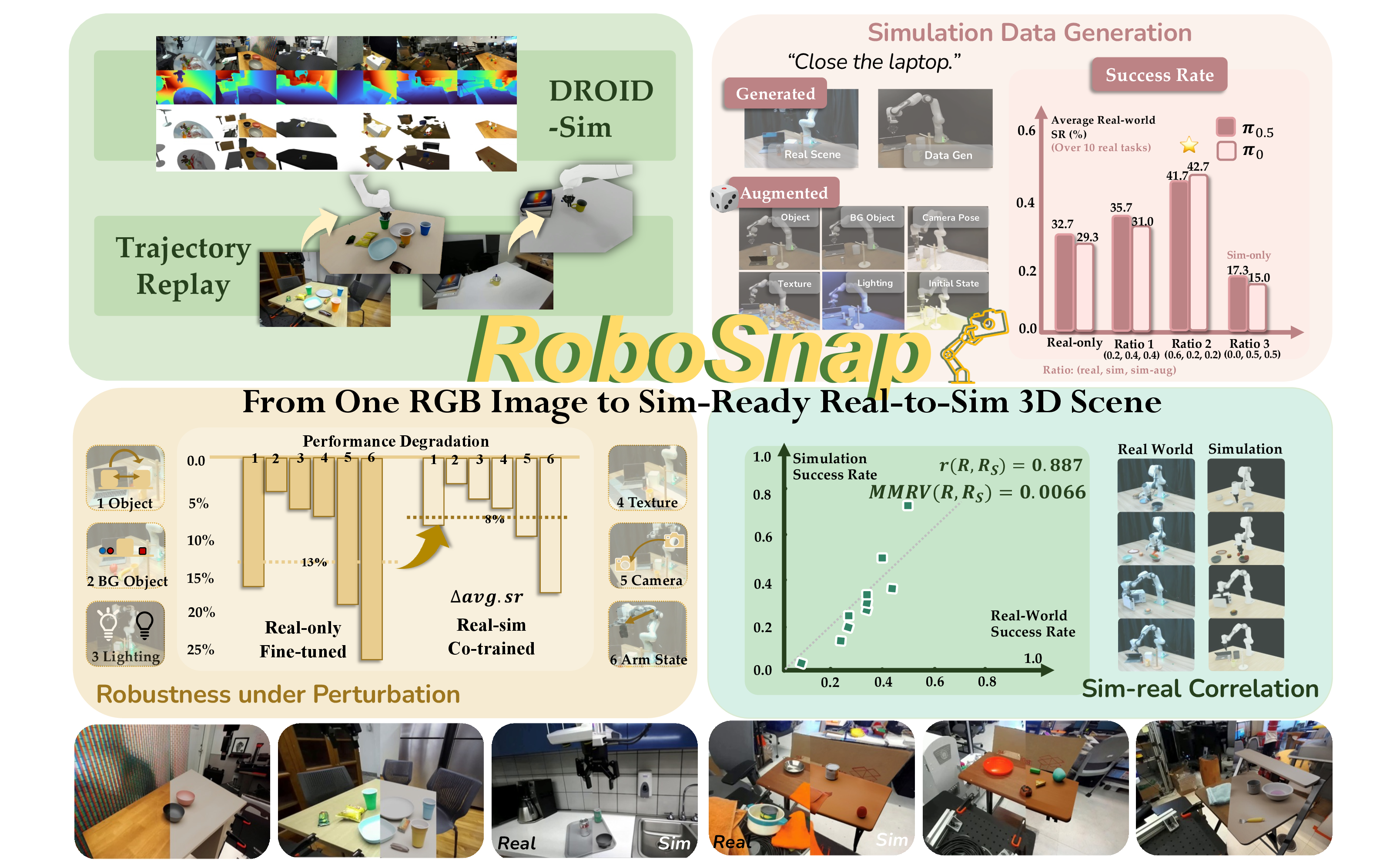
Recovering real-world scenes as interactive simulation environments can enable generalizable robot learning and reproducible policy evaluation. However, constructing scenes that are both physically stable and visually faithful remains slow and expensive. In this work, we present RoboSnap, a real-to-sim framework that turns a single RGB image into a simulation-ready scene. The key idea is a layered design that separates the physics-critical interaction area from the surrounding visual context: collision-aware foreground assets are refined for stable robot interaction, while a 3D Gaussian splatting visual layer preserves faithful background appearance under novel views. Experiments on DROID scenes and real-robot tasks show that RoboSnap achieves reliable trajectory replay in the recovered scenes, supports task-specific synthetic data generation for policy training, and yields meaningful sim-real correlation for policy evaluation. To further support real-to-sim research, we introduce DROID-Sim, a real-to-sim companion dataset constructed from 564 real-world scenes in DROID. Extensive experiments suggest that the value of real-to-sim methods lies not only in high-fidelity visual reconstruction, but in turning real environments into reusable infrastructure for robot learning and evaluation.
1 Introduction↩︎
Recent robot foundation models formulate manipulation as a conditional action generation task from visual, linguistic, and proprioceptive inputs [1]–[5]. As these models scale, large-scale training data and reproducible evaluation have become critical bottlenecks. Although real-world datasets and benchmarks provide substantial physical demonstrations and standardized protocols [6]–[9], scalable data acquisition and flexible policy evaluation remain costly, labor-intensive, and hardware-bound. Simulation offers a complementary path for scalable data synthesis, scene augmentation, and repeatable policy assessment, thereby motivating the construction of interactive simulation scenes that are both physically plausible and visually faithful to real-world deployment environments.
Existing approaches only partially satisfy these requirements. Procedural and generative scene synthesis methods have scaled simulatable environments for robot learning [10]–[14], but they primarily focus on creating diverse simulation scenes rather than recovering reusable interactive replicas of specific in-the-wild real-world scenes. Reconstruction-based real-to-sim methods improve scene alignment but often require multi-view capture or manual refinement [15]–[19]. Recent single-image systems reduce the capture burden [20]–[22], but their outputs typically target narrower endpoints: retrieval-based digital cousins, task or demonstration synthesis, or partially recovered scenes with static background. As a result, they do not generally recover persistent simulation worlds that can be re-rendered, edited, and reused from new viewpoints, and their effectiveness in downstream robot learning and evaluation workflows remains underexplored. Motivated by recent advances in monocular 3D geometry and image-conditioned 3D asset generation [23]–[26], we ask: Can we reconstruct a physically plausible, visually faithful, and simulation-ready environment from a single RGB image?
To this end, we present RoboSnap, a single-image real-to-sim method for manipulation scene generation. RoboSnap reconstructs the interaction area as collision-aware objects and support surfaces, aligns the area to a gravity-consistent frame, and refines object poses to resolve floating artifacts, interpenetrations, and unstable contacts. The surrounding context is modeled as a separate visual layer using background completion, Gaussian splatting, and scene lighting. The resulting scene is editable, reusable, and simulation-ready for robot data generation and evaluation.
We make the following contributions. (i) We propose RoboSnap, a layered real-to-sim method that converts a single RGB image into a simulation-ready scene. (ii) We systematically validate that the resulting scenes support downstream robot-learning workflows, including trajectory replay, data generation, and policy evaluation with meaningful correlation to real-world performance. (iii) We introduce DROID-Sim, a real-to-sim companion dataset of 564 DROID scenes [6], extending an existing robot dataset from recorded trajectories and images to reusable simulation environments.
2 Related Work↩︎
2.0.0.1 3D Generation and Scene Synthesis.
Procedural and generative scene-construction systems have scaled simulatable environments for robot learning, from everyday manipulation scenes to physically interactable tabletop and indoor layouts [11], [12], [27]–[30]. However, they typically synthesize new environments rather than reconstructing site-specific real-world robot scenes. Meanwhile, advances in monocular geometry and image-conditioned 3D asset generation enable 3D structure inference from limited visual inputs [23], [25], [26], [31], [32]; RoboSnap leverages these advances for real-to-sim, converting a single image into a physically plausible and visually faithful simulation environment.
2.0.0.2 Real-to-Sim-to-Real.
Real-to-sim methods reconstruct digital twins or task-specific simulation assets from real observations for policy learning and evaluation [15]–[19], [33]–[35]. Their alignment gains, however, typically come from additional information or intervention beyond a single RGB image, making such methods less lightweight and harder to reuse across different scenes. Recent single-observation methods reduce the capture burden [20]–[22], [36], but they often target narrower endpoints such as asset retrieval, static reconstruction, or demonstration synthesis, rather than producing reusable simulation worlds and validating the recovered scenes in downstream robot-learning workflows. RoboSnap instead reconstructs a single RGB image as a layered, physically refined manipulation scene that can be re-rendered, edited, and reused from new viewpoints.
2.0.0.3 Robot Data Generation and Policy Evaluation.
Large robot datasets provide foundational data for scalable training and reproducible evaluation [6]–[9], while generalist policies further motivate standardized benchmarks across diverse tasks [1]–[5]. Recent work has expanded robot datasets using generative visual methods [37]–[42] or simulation- and task-construction approaches [16], [43]–[46]. Several simulation benchmarks provide standardized tasks and environments for robot evaluation [9], [19], [27], [28], [47]–[50], and well-constructed simulated scenes can yield meaningful correlations with real-world policy performance. RoboSnap complements these efforts by converting real in-the-wild scene images, whether from robot datasets or casual captures, into reusable, simulation-ready environments for trajectory-based data generation and flexible policy evaluation.
3 Method↩︎
3.1 Layered Scene Reconstruction from a Single Image↩︎
3.1.0.1 Problem formulation.
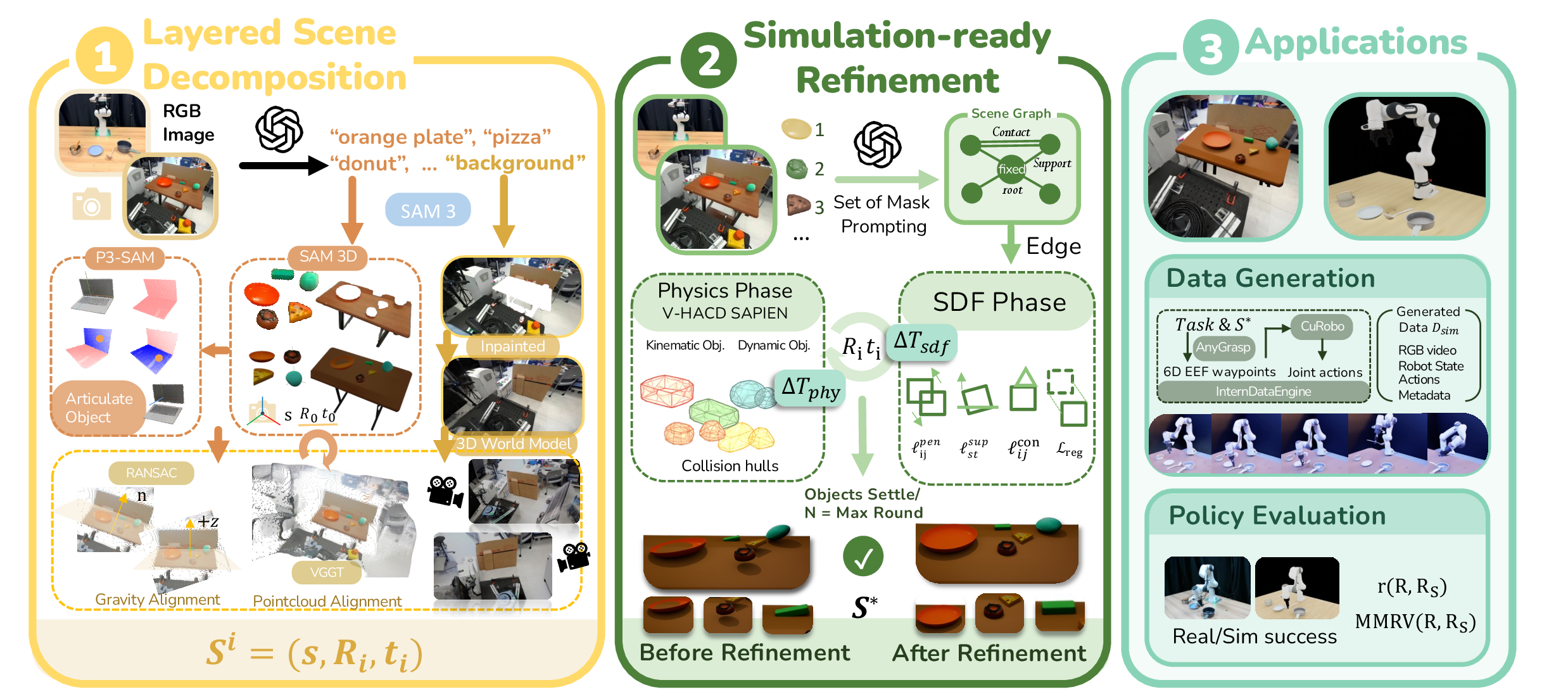
Given a single RGB image \(I\in\mathbb{R}^{H_0\times W_0\times 3}\), RoboSnap first reconstructs an initial layered scene \(\mathcal{S}^{(0)}\) and then refines it into a simulation-ready scene \(\mathcal{S}^{\star}\). The scene contains a physical layer of interactable objects and support surfaces, and a visual layer for the surrounding context. Both layers are registered to a canonical world frame \(W\), whose origin is the support-platform centroid with \(-\hat{\mathbf{e}}_z\) as the gravity direction.
3.1.0.2 Interactive Physical Layer.
We use a VLM [51] to parse the interaction area and identify object names \(\{\ell_i\}_{i=1}^{N}\), including the support platform. SAM 3 [52] extracts instance masks \(\{M_i\}_{i=1}^{N}\), and SAM 3D [25] reconstructs each object as a textured mesh \(\mathcal{M}_i\) with an initial pose and scale. To further register these object assets to the scene geometry, we use VGGT [23] to predict camera geometry, confidence, and a dense point map \(\mathcal{X}_V\) in the camera frame \(V\). For each object mask, we extract high-confidence foreground points from the VGGT point map and refine the initial SAM 3D pose using mask-guided registration. In practice, we perform coarse-to-fine fixed-scale ICP between sampled mesh surface points and the corresponding foreground point cloud, and reject updates with excessive rotation or translation. The resulting aligned pose is denoted as \(T_{i\to V}^{\mathrm{init}}\).
3.1.0.3 Canonical Alignment and Robot Base.
We estimate \(W\) from the dominant support platform by selecting support points from \(\mathcal{X}_V\) and fitting a plane with RANSAC followed by least-squares refinement. \(T_{V\to W}\) aligns the plane normal to \(\hat{\mathbf{e}}_z\) and places the support-platform centroid at the origin. Object poses are lifted to \(W\) by \[T_{i\to W}^{\mathrm{init}} = T_{V\to W}T_{i\to V}^{\mathrm{init}} . \label{eq:obj-to-W}\tag{1}\] For calibrated datasets such as DROID [6], the robot base is placed using the camera-frame base pose: \(T_{B\to W}=T_{V\to W}T_{B\to V}.\) For uncalibrated captures, the robot base can be initialized from the support-platform geometry and a specified robot-facing direction.
3.1.0.4 Visual Context Layer.
We reconstruct the non-interactable context separately. After foreground masking, we inpaint missing regions using a VLM-guided prompt (Appendix 8.1.1) and pass the completed image to a generative world model [53], producing a Gaussian-splat scene \(\mathcal{G}_M\) in frame \(F_M\). We align \(\mathcal{G}_M\) to \(V\) using sparse correspondences and ICP, then lift it to \(W\) with \(T_{F_M\to W}=T_{V\to W}T_{F_M\to V}.\)
3.1.0.5 Articulated Objects.
For articulated objects, we decompose the reconstructed mesh into semantic parts using a point-based part segmentation model [54], split the mesh by estimated part boxes, and attach the recovered part meshes to category-level kinematic parameters retrieved from an articulated-object dataset [55].
Collecting these components, we denote the initial layered scene as \(\mathcal{S}^{(0)}=(\{(M_i,\ell_i,\mathcal{M}_i,T_{i\to W}^{\mathrm{init}})\}_{i=1}^{N},(\mathcal{G}_M,T_{F_M\to W}),W,T_{B\to W})\).
3.2 Simulation-ready Refinement↩︎
Independent per-object pose estimates often produce floating objects, interpenetrations, and unstable contacts. We therefore extract a physical scene graph and refine object poses with an alternating SDF–physics procedure: the SDF phase enforces support/contact constraints and resolves geometric conflicts, while the physics phase settles objects under gravity.
3.2.0.1 Scene Graph Extraction.
Inspired by CAST [21], we infer pairwise physical relations with Set-of-Mark prompting [56] and a VLM [51]. From the instance masks and captions in §3.1, GPT-4V predicts relations over \(K=5\) randomized SoM overlays. Majority-voted predictions define directed Support edges and bidirectional Contact edges, yielding \(\mathcal{G}_{\mathrm{phys}}=(\mathcal{V},\mathcal{E}_{\mathrm{sup}}\cup\mathcal{E}_{\mathrm{con}})\). Objects that only support others are fixed as roots \(\mathcal{R}\).
3.2.0.2 Alternating SDF–physics Optimization.
Given \(\mathcal{G}_{\mathrm{phys}}\) and initial poses \(\{T_{i\to W}^{\mathrm{init}}\}\) from Eq. 1 , we refine non-root object poses by optimizing residual SE(3) updates: \[T_{i \to W} = \Delta T_i T_{i\to W}^{\mathrm{init}}, \qquad \Delta T_i = \begin{bmatrix} \exp([\Delta\mathbf{r}_i]_\times) & \Delta\mathbf{t}_i\\ \mathbf{0}^{\top} & 1 \end{bmatrix}, \quad i\notin\mathcal{R}. \label{eq:delta-pose}\tag{2}\] The refinement alternates between an SDF optimization phase and a physics settling phase. The SDF phase uses precomputed SDF grids and surface samples to minimize penetration, support, contact, and regularization losses, with full formulae in Appendix 8. The physics phase decomposes meshes into V-HACD collision hulls [57] and simulates them in SAPIEN [55], keeping root objects kinematic and other objects dynamic. The settled poses initialize the next SDF phase, and the final poses define \(\mathcal{S}^{\star}\).
3.3 Robot Data Generation and Evaluation↩︎
The refined scene \(\mathcal{S}^{\star}\) supports trajectory replay, task-specific data generation, and closed-loop policy evaluation.
3.3.0.1 Layered Rendering.
For a query camera \(Q\), Isaac Sim [58] renders the physical layer as \((I_{\mathrm{fg}},D_{\mathrm{fg}},\alpha_{\mathrm{fg}})\), while the visual layer is rendered from the same camera transformed to the Gaussian splatting frame, \(T_{Q\to F_M}=T_{F_M\to W}^{-1}T_{Q\to W}\), yielding \((I_{\mathrm{bg}},D_{\mathrm{bg}})\). We depth-composite the two layers as \[I_{\mathrm{out}}(\mathbf{u}) = m(\mathbf{u})I_{\mathrm{fg}}(\mathbf{u}) + (1-m(\mathbf{u}))I_{\mathrm{bg}}(\mathbf{u}), \quad m(\mathbf{u})= \mathbf{1}\!\left[ \alpha_{\mathrm{fg}}(\mathbf{u})>0 \wedge D_{\mathrm{fg}}(\mathbf{u})\le D_{\mathrm{bg}}(\mathbf{u}) \right]. \label{eq:compositing}\tag{3}\]
3.3.0.2 Trajectory-based Data Generation.
We instantiate \(\mathcal{S}^{\star}\) in an Isaac Sim-based data engine [46] with a task specification, robot embodiment, query cameras, and the layered renderer. Grasp-centric skills use AnyGrasp-initialized candidates [59]; skill modules output target end-effector 6D waypoints, which cuRobo converts into collision-aware dense joint-space actions [60].
3.3.0.3 Policy Evaluation.
For closed-loop evaluation, actions are executed in \(\mathcal{S}^{\star}\). For sim-real evaluation, let \(\mathbf{R}\) and \(\mathbf{R}_{S}\) denote real and simulated success-rate vectors over \(N\) tasks or checkpoints. We report Pearson correlation:
\[r(\mathbf{R},\mathbf{R}_{S})=\frac{\sum_i (R_i-\bar{R})(R_{S,i}-\bar{R}_S)}{\sqrt{\sum_i (R_i-\bar{R})^2}\sqrt{\sum_i (R_{S,i}-\bar{R}_S)^2}}\] to measure success-rate agreement, and mean maximum rank violation \[\mathrm{MMRV}(\mathbf{R},\mathbf{R}_S)=\frac{1}{N}\sum_i\max_j |R_i-R_j|\mathbf{1}[(R_{S,i}<R_{S,j})\neq(R_i<R_j)]\] to measure rank-order inconsistency. Higher \(r\) and lower MMRV [50] indicate better sim-real alignment.
4 Experiments↩︎
We organize our experiments around five questions that probe what single-image real-to-sim scene recovery can support in robot learning and evaluation:
Are the reconstructed scenes visually faithful to the input image and physically stable in simulation?
Do the recovered scenes preserve the geometry and contact structure needed to replay real robot trajectories?
Can RoboSnap-generated scenes improve real-world policy performance through task-specific data generation?
Are policies trained with RoboSnap-generated data robust to real-world perturbations?
Can RoboSnap scenes serve as a generative evaluation harness whose simulated rollouts correlate with real-world policy performance?
4.1 Visual Realism and Simulation Stability↩︎
4.1.0.1 Scene Sampling.
We construct DROID-Sim by running RoboSnap on 564 DROID scenes. For detailed quantitative evaluation and baseline comparison, we use a fixed subset of 10 scenes that covers diverse tabletop layouts and object categories. Additional details on DROID-Sim are provided in Appendix 9.
4.1.0.2 Visual Alignment.
We compare alignment to the input image with RoLA [22] under the same single-frame setting, using each method’s respective segmentation and reconstruction pipeline. Since RoboSnap reconstructs the full interaction region rather than preserving large background areas, PSNR and LPIPS [61] show only modest differences, while other metrics in Figure 3 indicate better preservation of scene structure, color, and texture distribution. Metric definitions are in Appendix 7.1.1.

4.1.0.3 Simulation Readiness.
We define a scene as simulation-ready if it remains physically stable without severe floating or interpenetration after being loaded into a simulator. We import each reconstruction into Isaac Sim [58] and run the physics simulation for 300 frames. RoboSnap substantially improves stability metrics (Table 1), supporting downstream robot interaction and policy evaluation (Q1). Metric definitions are in Appendix 7.1.2.
| Method | Falling \(\downarrow\) | Collision \(\downarrow\) | Trans MSE \(\downarrow\) | Mean disp. (m) \(\downarrow\) | Quat MSE \(\downarrow\) |
|---|---|---|---|---|---|
| SAM 3D [25] | 0.5640 | 0.3590 | 0.1079 | 0.3284 | 0.1560 |
| SAM 3D + FoundationPose [62] | 0.5900 | 0.1538 | 0.1921 | 0.4383 | 0.1703 |
| RoLA [22] | 0.3810 | 0.3226 | 0.0736 | 0.2713 | 0.1093 |
| w/o refinement | 0.4320 | 0.2982 | 0.0977 | 0.3126 | 0.1255 |
| (ours) | 0.1026 | 0.0256 | 0.0022 | 0.0474 | 0.0178 |
4.2 Trajectory Replay↩︎
We evaluate replay on 5 randomly sampled scenes from the 10 in §4.1 using the original DROID trajectories.
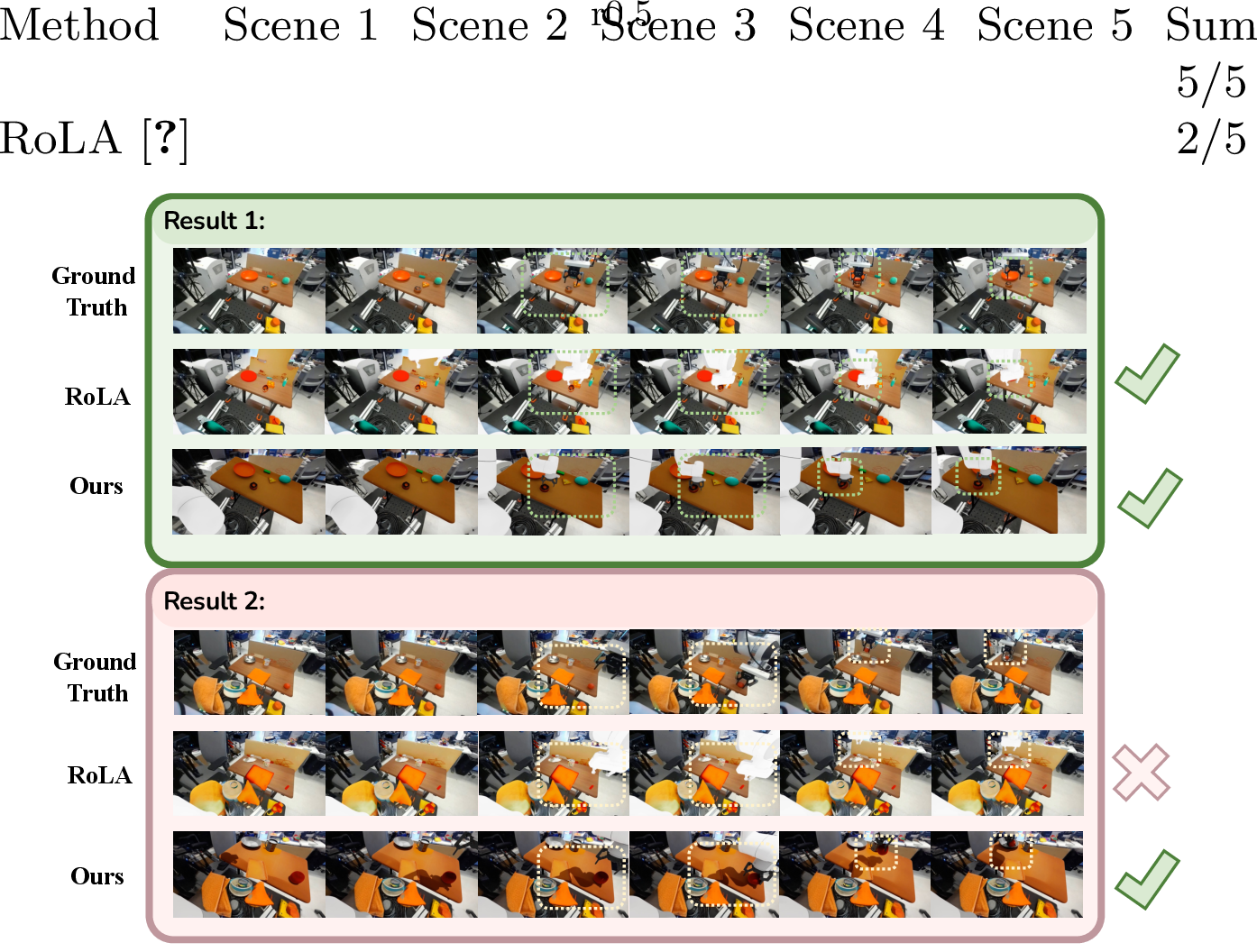
This evaluation differs from demonstration-driven real-to-sim pipelines such as ReBot [37] and RialTo [15]. These methods use demonstration signals, such as gripper trajectories or real-policy rollouts, to place objects or collect privileged trajectories in simulation. In contrast, our replay experiment evaluates the recovered scene itself (Q2): objects are instantiated from the layout generated by RoboSnap.
A replay trial succeeds if the gripper grasps the intended object and moves it to the target without interpenetration or collisions. We compare with RoLA [22], a similar single-image scene recovery method that can support replay when action trajectories are given. Successful rollouts indicate that the recovered layout and robot base are accurate enough to reproduce key contact events in the original demonstration.
4.3 Robot Data Generation↩︎
We next explore whether demonstrations generated from RoboSnap scenes improve performance on user-defined tasks (Q3).
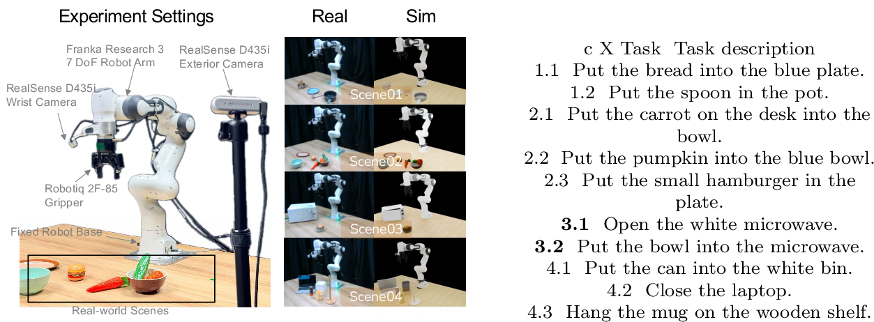
Across four real setups, we fine-tune \(\pi_{0.5}\) [5] and \(\pi_0\) [4] under a real-only baseline and three streamed data-mixture settings over (real demonstrations, RoboSnap-generated demonstrations, simulation-augmented demonstrations): R1=\((0.2,0.4,0.4)\), R2=\((0.6,0.2,0.2)\), and R3=\((0,0.5,0.5)\). For each task, we collect 30 real demonstrations and evaluate each policy over 30 real-world trials. Detailed data synthesis and experiment settings are provided in Appendix 7.3.
Ratio 2 yields the best average performance, improving success from 32.7% to 41.7% for \(\pi_{0.5}\) and from 29.3% to 42.7% for \(\pi_0\) as shown in Table 2. Ratio 3 still achieves nonzero real-world success without real demonstrations. These results show that RoboSnap scenes can generate useful task-specific data for real-world policy fine-tuning (Q3).
| Task | \(\pi_{0.5}\) | \(\pi_0\) | ||||||
|---|---|---|---|---|---|---|---|---|
| 2-5(lr)6-9 | Real | R1 | R2 | R3 | Real | R1 | R2 | R3 |
| 1.1 | ||||||||
| 1.2 | ||||||||
| 2.1 | ||||||||
| 2.2 | ||||||||
| 2.3 | ||||||||
| 3.1 | ||||||||
| 3.2 | ||||||||
| 4.1 | ||||||||
| 4.2 | ||||||||
| 4.3 | ||||||||
| Average | 32.7 | 35.7 | 41.7 | 17.3 | 29.3 | 31.0 | 42.7 | 15.0 |
1.2pt
4.4 Randomization↩︎
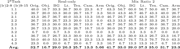
Simulation enables controlled data augmentations that are costly to reproduce physically. We evaluate whether policies fine-tuned with RoboSnap-generated data retain performance under six real-world perturbations: object pose (Obj., \(\pm\)10 cm), background objects (BG), lighting (Lt.), table texture (Tex.), camera pose (Cam.), and robot initial state (Arm). We use \(\pi_{0.5}\) performance under Ratio 2 from §4.3. Detailed settings are provided in Appendix 7.4.
Table ¿tbl:fig:robust? reports the relative success-rate degradation from the original setting. Real-sim co-training reduces the average degradation from 13% to 8% across perturbation types, with clear gains under camera-pose and robot-initial-state shifts. These results show that data generated in RoboSnap scenes improves robustness retention under real-world perturbations (Q4).
4.5 Generative Evaluation Harness↩︎
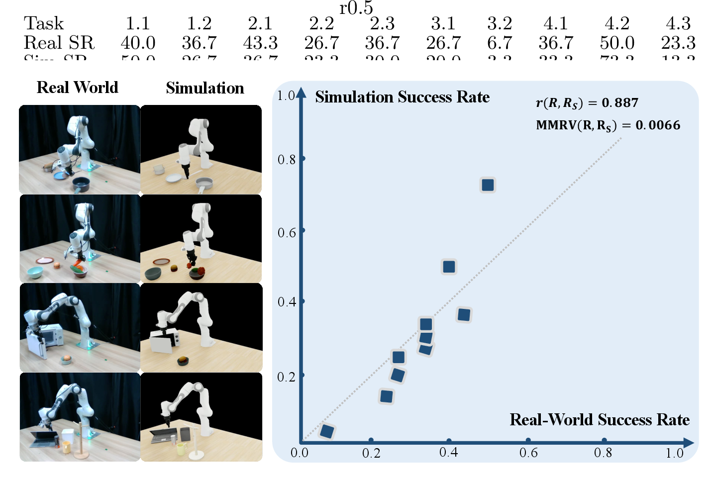
Generative evaluation (Q5) refers to flexible policy evaluation through synthetic environments. This is challenging for manipulation since embodied evaluation depends on both visual realism and contact dynamics. To assess whether RoboSnap scenes can serve as a generative evaluation harness, we run the real-only fine-tuned \(\pi_{0.5}\) policies from §4.3 in the corresponding generated scenes and compare real-world and simulation success rates.
The resulting Pearson correlation (\(r=0.887\)) and MMRV (\(\text{0.0066}\)) indicate that RoboSnap captures sufficient sim-real correlation and task-relevant dynamics, which can provide a simulation proxy for real-world manipulation evaluation.
5 Conclusion↩︎
We presented RoboSnap, a single-image real-to-sim method that reconstructs scenes that can be re-rendered, edited, and reused from new viewpoints. By separating interactive physical objects from visual context and refining object poses for simulation stability, RoboSnap produces scenes that are both visually faithful and physically stable. Our experiment results show that the recovered RoboSnap scenes can support faithful replay, generate useful robot data, and serve as a reliable evaluation harness for real-world manipulation. We view this as a beneficial trial toward treating real-world scene reconstruction not merely as building visual digital-twin, but as reusable infrastructure for embodied training and evaluation.
6 Limitations↩︎
(1) Input Quality. RoboSnap reconstructs reusable scenes from single-RGB captures. Therefore, inputs of extreme low quality like severe occlusion, extreme lighting, and visually ambiguous materials can reduce reconstruction quality or reliability of generated demonstrations.
(2) Object and Physics Regime. The current system focuses on rigid and articulated objects with well-defined support/contact structure. In this work, we do not target deformable, granular, or fluid materials, whose behavior is not well captured by rigid-body simulation models and is beyond the scope of this work.
(3) Parameter Estimation Pipeline. The system does not include a dedicated pipeline for automatic physical parameter estimation. Parameters such as friction and mass are inferred from VLM prior knowledge, while joint parameters for articulated objects are retrieved from objects of the similar type in the standard dataset.
(4) Further Validation. Since RoboSnap outputs a simulator-level scene rather than policy-specific data or labels, the same scene interface can in principle support different manipulation policies including video/world-model-based structures. Given our training and evaluation budget, we validate this interface on the settings and models in this paper and plan to leave broader framework validation to future work.
7 Experiment↩︎
7.1 Metrics↩︎
7.1.1 Visual-alignment metrics↩︎
We evaluate visual alignment by comparing each method’s rendered RGB image \(\hat{I}\) to the original DROID frame \(I\), resizing rendered images to match the ground-truth resolution with bicubic interpolation. We report six complementary metrics: pixel fidelity, structure, perceptual similarity, local geometry, color distribution, and texture statistics.
7.1.1.1 Pixel, structure, and perceptual metrics.
PSNR is computed from RGB MSE after normalizing to \([0,1]\): \[\mathrm{MSE} = \frac{1}{3|\Omega|} \sum_{\mathbf{u}\in\Omega}\sum_{c\in\{r,g,b\}} (I_c(\mathbf{u})-\hat{I}_c(\mathbf{u}))^2,\quad
\mathrm{PSNR} = 20\log_{10}\frac{1}{\sqrt{\mathrm{MSE}}}.\] SSIM uses skimage.metrics.structural_similarity on uint8 RGB images; LPIPS-Alex uses the official AlexNet implementation on \([-1,1]\) scaled
RGB. Higher PSNR/SSIM and lower LPIPS-Alex indicate better agreement.
7.1.1.2 Local-feature, color, and texture metrics.
SIFT match ratio is computed on grayscale \(640\times360\) images with up to 800 keypoints per image, using brute-force \(\ell_2\) KNN matching and Lowe’s 0.75 ratio test: \[\mathrm{SIFT\text{-}MR} = \frac{N_{\mathrm{good}}}{\min(N_I,N_{\hat{I}})+\epsilon}.\] RGB-Wasserstein compares 64-bin histograms per channel via \(W_1\): \[\mathrm{RGB\text{-}W} = \frac{1}{3}\sum_c W_1(p_c,\hat{p}_c),\quad\text{lower is better.}\] Gabor-\(\ell_1\) uses \(K=24\) filters (8 orientations × 3 wavelengths) on \(256\times144\) grayscale images; filter response energies are \(\ell_2\)-normalized and compared by \[\mathrm{Gabor\text{-}\ell_1} = \frac{1}{K}\Big\|\frac{\mathbf{e}(I)}{\|\mathbf{e}(I)\|_2+\epsilon}-\frac{\mathbf{e}(\hat{I})}{\|\mathbf{e}(\hat{I})\|_2+\epsilon}\Big\|_1.\] Lower Gabor-\(\ell_1\) indicates closer texture-frequency agreement.
7.1.2 Simulation-Ready Metrics↩︎
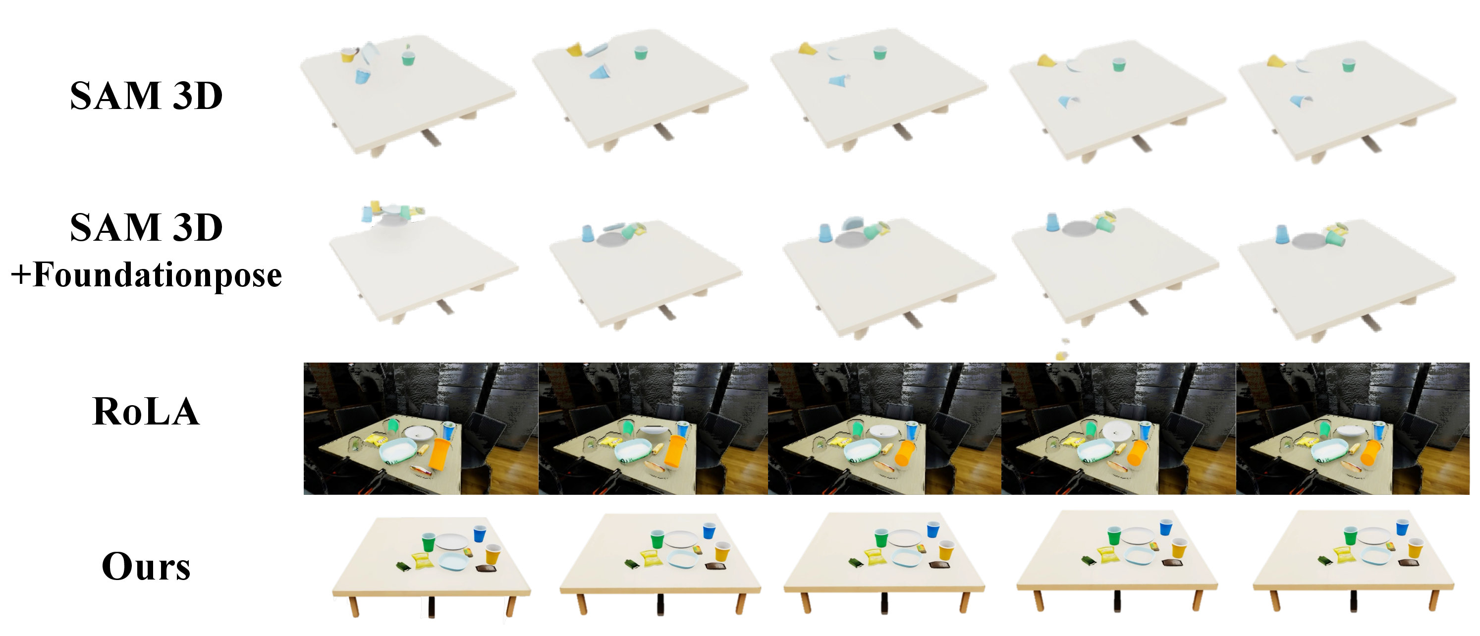
We measure whether a reconstructed scene is simulation-ready by first aligning it to a gravity-consistent coordinate frame. Specifically, we fit the dominant support plane with RANSAC and rotate the scene so that the fitted plane normal aligns with the simulator’s \(+z\) up axis, i.e., gravity acts along \(-z\). We then load all object USD assets into IsaacLab with the transformed recovered poses and collision geometry, and step \(T=300\) physics steps with gravity. Object root poses are sampled every 10 steps.
Let object \(i\) have poses \(\mathbf{x}_{i,t}=(\mathbf{p}_{i,t},\mathbf{q}_{i,t})\), with world-space center \[\mathbf{c}_{i,t} = \mathbf{p}_{i,t} + R(\mathbf{q}_{i,t})\,\mathbf{c}^{\mathrm{local}}_i, \quad \mathbf{c}^{\mathrm{local}}_i = R(\mathbf{q}_{i,0})^\top (\mathbf{c}_{i,0}^{\mathrm{world}} - \mathbf{p}_{i,0}).\] Translation drift and per-object metrics are \[\Delta \mathbf{c}_i = \mathbf{c}_{i,T}-\mathbf{c}_{i,0},\quad \mathrm{TransMSE}_i = \frac{1}{3}\|\Delta \mathbf{c}_i\|_2^2,\quad \mathrm{Disp}_i = \|\Delta \mathbf{c}_i\|_2.\] Rotation drift is computed after sign-correcting quaternions: \[\tilde{\mathbf{q}}_{i,T} = \begin{cases} \mathbf{q}_{i,T}, & \mathbf{q}_{i,0}^{\top}\mathbf{q}_{i,T} \ge 0,\\ -\mathbf{q}_{i,T}, & \mathbf{q}_{i,0}^{\top}\mathbf{q}_{i,T} < 0 \end{cases},\quad \mathrm{QuatMSE}_i = \frac{1}{4}\|\tilde{\mathbf{q}}_{i,T}-\mathbf{q}_{i,0}\|_2^2.\]
Falling is flagged if the tilt angle of the object’s local up exceeds \(45^\circ\): \[\phi_i = \cos^{-1}\frac{\mathbf{u}_{i,0}^{\top}\mathbf{u}_{i,T}}{\|\mathbf{u}_{i,0}\|_2\|\mathbf{u}_{i,T}\|_2},\quad \mathbf{u}_{i,t}=R(\mathbf{q}_{i,t})(0,0,1)^\top.\] Collision/pop-out failures are detected if consecutive center displacements exceed 0.05 m or upward jumps exceed 0.03 m. Scene-level metrics report fractions of falling/collision objects, mean Trans MSE, mean center displacement, and mean quaternion MSE. These jointly measure physical stability and simulation readiness.
7.2 Trajectory Replay↩︎
We evaluate whether a recovered static scene can support open-loop replay of the original DROID trajectory. For each sampled scene, we instantiate the recovered objects, collision assets, gravity-aligned scene frame, and robot base in IsaacLab, then replay the recorded gripper trajectory in the recovered robot/world frame.
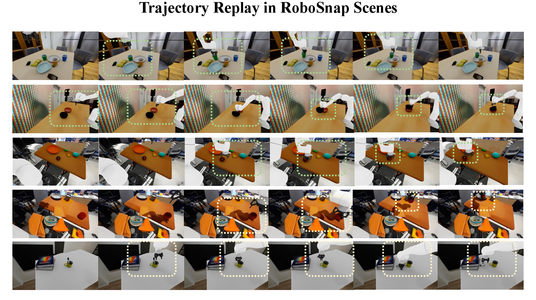
The trajectory is used only for evaluation: we do not optimize object poses from replay outcomes or use privileged simulation rollouts to repair failures. A trial succeeds if the gripper grasps the intended object and moves it to the target region without severe collision, interpenetration, or contact failure.
This test differs from simulation data generation with real-world replay and demonstration-driven real-to-sim pipelines. Rather than generating trajectories in simulation and transferring them to the real world, or using demonstrations to fit object placements, we ask whether an existing real trajectory becomes executable once the static scene, object layout, and robot base are accurately recovered. Thus, replay success measures active interaction fidelity of the reconstructed scene and suggests a low-cost path for augmenting real robot logs through simulation replay, perturbation, and re-rendering.
The replay experiment evaluates whether a reconstructed static scene can support the original contact sequence from a real demonstration. For each scene, we instantiate reconstructed objects with their recovered poses and collision geometry, place the robot using the robot-base transform in the dataset. Therefore, replay success primarily reflects the accuracy of scene recovery.
7.3 Real Scene Tasks↩︎
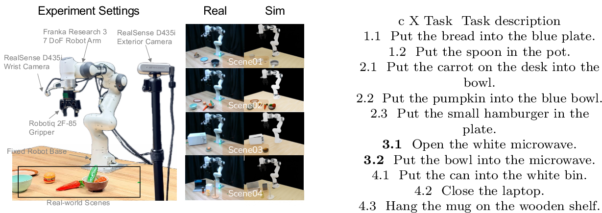
7.3.1 Training Details↩︎
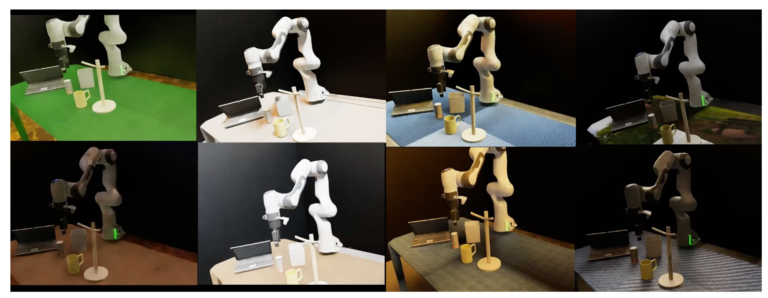
For each task, we convert both real and generated trajectories into the RLDS format used by the OpenPI framework. The real-only baseline is initialized from the corresponding pretrained checkpoint and fine-tuned using 30 real demonstrations. For mixed-data settings, we additionally stream from two task-specific synthetic pools generated in the corresponding RoboSnap scene: simulation-generated demonstrations and simulation-augmented demonstrations. Each synthetic source contains 2,000 demonstrations per task. The simulation-augmented pool is evenly balanced across six perturbation types: manipulated-object displacement, background objects, lighting, camera pose, robot-arm initial state, and table texture.
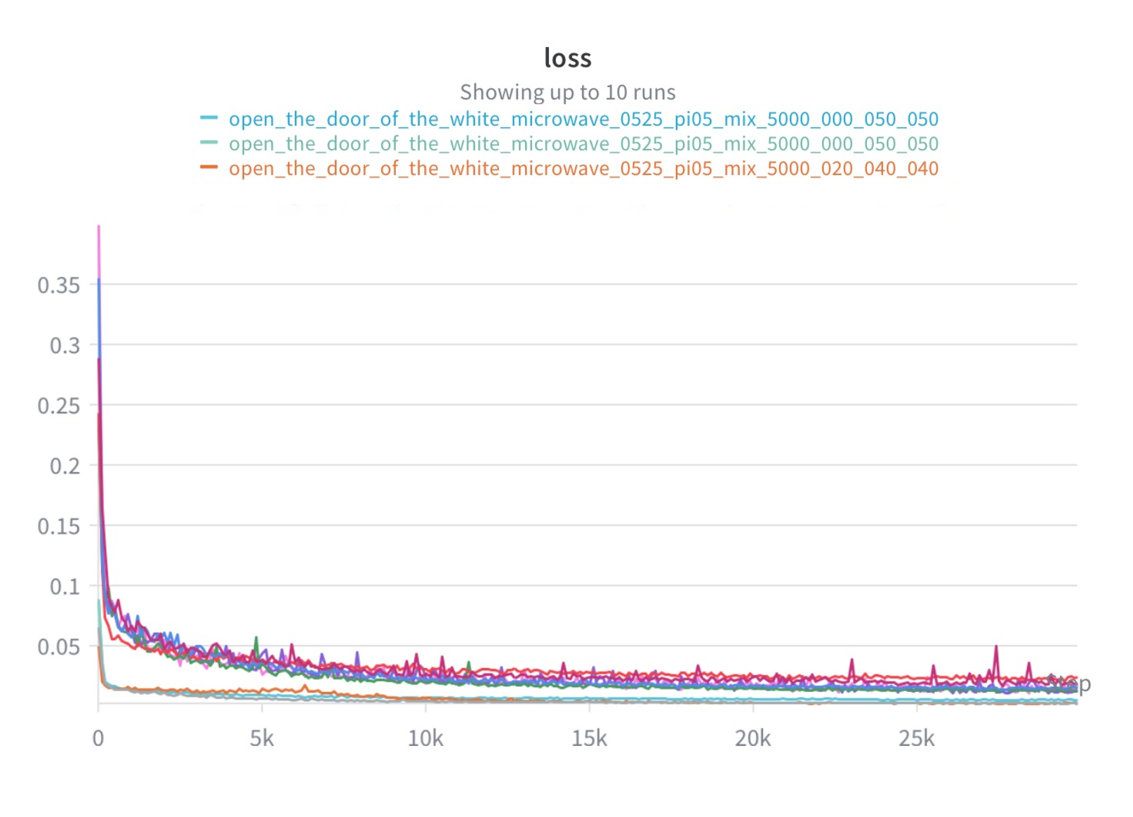
All settings use the same optimization budget: batch size 16, a cosine learning-rate schedule with 100 warmup steps and peak learning rate \(2\times10^{-5}\). We evaluate all methods at the fixed 15k-step checkpoint according to Figure 10.
Data mixtures are implemented by streaming from the real, simulation-generated, and simulation-augmented RLDS sources with the specified weights. Thus, R1–R3 only change the expected source composition of consumed mini-batches, while keeping the number of gradient updates, batch size, model initialization, action space, and evaluation protocol fixed. We use joint-position actions with action horizon 16 for \(\pi_{0.5}\), and use the corresponding OpenPI fine-tuning configuration for \(\pi_0\).
For both \(\pi_0\) and \(\pi_{0.5}\), the logged training loss is the OpenPI action-generation objective rather than a task-success metric. Given an observation \(o\) and a ground-truth action chunk \(a\), the model samples Gaussian noise \(\epsilon\) and a time \(t\), constructs \[x_t = t\epsilon + (1-t)a, \qquad u_t = \epsilon - a,\] and predicts the velocity target \(u_t\) from \((o,x_t,t)\). The reported scalar loss is \[\mathcal{L} = \mathbb{E} \left[ \left\| v_\theta(o,x_t,t)-u_t \right\|_2^2 \right],\] averaged over action dimensions, action horizon, and mini-batch samples. Therefore, the loss curves are used as optimization diagnostics.
7.3.2 Synthetic Data Generation↩︎
We modify the InternDataEngine [46] to improve the sim-to-real performance. Specifically, we filter out irrational IK-based pick poses that are unlikely to succeed on real hardware. We also generate more regularized place poses by keeping them aligned with the preceding poses, which improves task success rate, accelerates trajectory generation, and further enhances transferability from simulation to the real world. These optimizations enable large-scale data generation, reaching approximately 10,000 task-specific trajectories per day on 8 RTX 4090 GPUs.
For each real setup, we export the recovered RoboSnap scene into a task-generation configuration. The configuration bridges the recovered scene and the data-generation engine: it specifies the scene assets, robot and camera setup, task instruction, target objects, skill template, and output format, which makes the task definition and trajectory synthesis flexible enough. A simplified example is shown below.
task: name: <scene-task-id> scene: asset_root: <robosnap-scene-root> arena_file: <arena-config>
robot: name: franka config: <robot-config> base_pose: <recovered-base-pose>
cameras: wrist: <wrist-camera-config> exterior: <exterior-camera-config>
objects: target: asset: <recovered-object-usd> pose: <recovered-world-pose> receptacle: asset: <recovered-object-usd> pose: <recovered-world-pose>
generation: instruction: <task-language-instruction> target_object: target support_region: <task-specific-region> skill_sequence: - <pick/place/close/open-skill-template>
output: task_dir: <output-directory> save: - rgb - robot_state - actions - camera_params - metadata
InternDataEngine loads this configuration to instantiate the recovered scene in Isaac Sim [58], attach the specified robot and cameras, and execute the skill sequence under the language instruction. The generation pipeline samples task-relevant object poses or grasp candidates, produces 6-DoF end-effector waypoints, converts them into collision-aware robot actions, and saves successful rollouts as task-specific simulated demonstrations.
7.3.3 Real World Evaluation↩︎
We evaluate all policies on the physical Franka Research 3 setup with a Robotiq 2F-85 gripper. The robot model used in simulation is the standard Franka–Robotiq asset rather than a reconstructed or Gaussian-splat asset. A trial is counted as successful only if the task reaches the completion state specified by the language instruction and remains stable at the end of execution. For non-long-horizon tasks, partial completion is counted as failure; for the long-horizon microwave task, the two stages are evaluated separately as Tasks 3.1 and 3.2.
Before each trial, objects are reset to the prescribed initial positions and poses. Non-long-horizon trials are executed for at most 2,000 inference steps, while long-horizon trials are executed for at most 5,000 steps. If the task is not completed within the step budget, or if execution is aborted due to unsafe motion, severe collision, or invalid robot state, the trial is marked as failure. Each setting is evaluated with three batches of 10 trials, and we compute summary statistics over the three 10-trial runs.
7.4 Real-World Robustness Perturbations↩︎
Starting from the original evaluation setup (Orig.), we introduce six controlled real-world perturbations to test policy robustness while keeping the task instruction and target object identity fixed.
In the object-pose condition (Obj.), the manipulated object is translated by approximately 10 cm along a fixed direction before rollout.

In the background condition (BG), additional distractor objects, including cubes and fruit, are placed on the table. In the lighting condition (Light), the room light is turned off to change image illumination. In the texture condition (Tex.), the table appearance is changed by covering it with the same tablecloth across trials. In the camera condition (Cam.), the camera is moved to another fixed viewpoint. In the robot initial-state condition (Arm.), the end-effector is first driven to a fixed alternative starting pose before executing the policy. Each perturbation is applied independently, so performance changes can be attributed to a specific source of distribution shift.
7.5 Generative Evaluation Harness↩︎
7.5.0.1 Behavior-Space Diagnostics for Generative Evaluation.
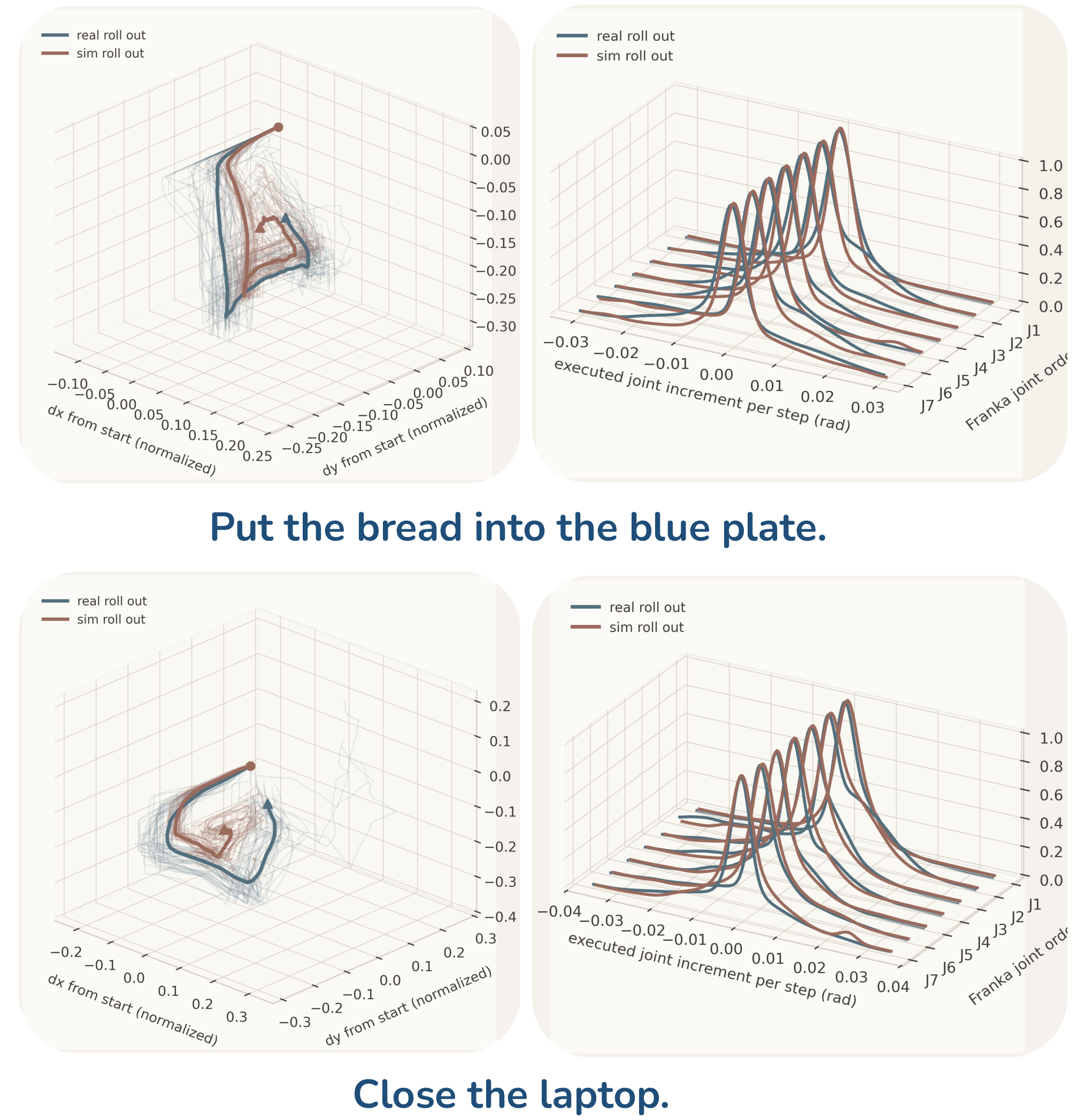
Beyond success-rate correlation, we analyze whether the generated scenes induce similar policy behavior in task space and action space. For each task, we execute the same real-only fine-tuned \(\pi_{0.5}\) policy in the real environment and in the corresponding RoboSnap-generated simulation scene, without additional adaptation. We record the end-effector trajectory and the executed Franka joint states during each rollout.
For task-space behavior, we express the end-effector trajectory as displacement from its initial position, \[\Delta \mathbf{p}_t = \mathbf{p}_t - \mathbf{p}_0,\] and normalize the displacement for visualization. This removes global offsets and highlights whether the simulated rollout follows the same interaction-relevant motion pattern as the real rollout. For action-space behavior, we compute the per-step executed joint increments \[\Delta q_t^j = q_{t+1}^j - q_t^j,\] for each Franka joint \(j\), and compare the normalized marginal distributions of \(\Delta q_t^j\) between real and simulated rollouts.
This diagnostic complements the aggregate sim-real correlation reported in Sec. 4.5. A generated scene may match visual appearance but still induce different behavior if the object layout, robot base, or contact geometry is inaccurate. Similar end-effector trajectories and joint-increment distributions indicate that RoboSnap scenes elicit comparable low-level control behavior from real-only trained policy, supporting their use as a generative evaluation proxy for real deployment of manipulation policies.
8 Method↩︎
8.1 Layered Scene Reconstruction from a Single Image↩︎
8.1.1 Background Inpainting↩︎
We use Gemini-2.5-flash-image [63] for background inpainting. Given a masked scene image where the interaction region is removed and only the background is retained, we use the following prompt to recover an empty background while preserving the scene geometry, camera perspective, and lighting.
You are an excellent image inpainter. Your task is to inpaint the masked image, where only the background is reserved and the interactive area has been removed.
Please remove all black regions from the scene, since they are not part of the background. Keep the room structure unchanged. Preserve walls, floor, ceiling, windows, and lighting to recover a full background image. Do not change the camera perspective. Return an empty background with consistent geometry and textures.
I stress again that I am asking you to inpaint the background, not refill the mask area. Make additional careful checks to avoid deleting any remaining background objects. If there are pixels from the interactive area that were not completely removed, remove them as well, leaving only the background.
Special reminder: remove the desktop area as well, since I generate the interaction area separately. I want the background to be empty so that it can hold the generated desk.
8.2 Simulation-ready Refinement↩︎

8.2.0.1 Simulation-ready Refinement Details.
Algorithm 15 summarizes the full procedure of the Simulation-ready Refinement. Typical hyperparameters are \(N_{\text{round}} = 20\), \(N_{\text{sdf}} = 15\), \(N_{\text{sim}} = 200\), \(N_{\text{damp}} = 100\), with convergence threshold \(\varepsilon = 10^{-4}\) on maximum object displacement. In the final round, simulation steps are increased \(5\times\) to ensure all objects have settled.
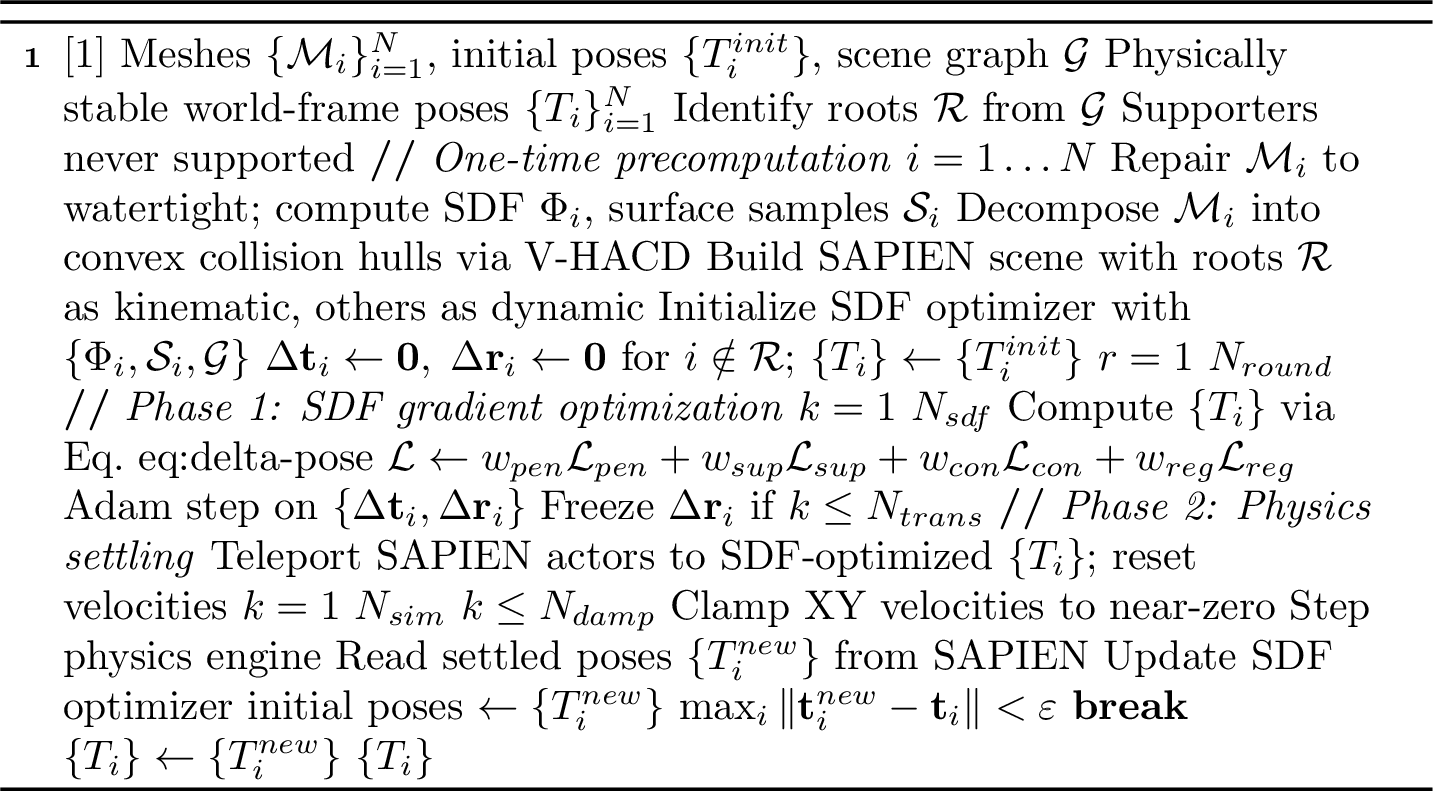
We provide the full formulations of the four loss terms used in the SDF phase of Algorithm 15. For each object \(i\), let \(\Phi_i(\mathbf{x})\) denote its precomputed signed distance field (negative inside, positive outside) and \(\mathcal{S}_i\) its set of \(M\) surface sample points, both in the local coordinate frame.
8.2.0.2 Penetration loss.
For every unordered pair \(\{i, j\}\), \(i \neq j\), we transform surface samples of \(j\) into \(i\)’s local frame and penalize negative SDF values: \[\ell_{ij}^{\text{pen}} \;=\; \frac{1}{M} \sum_{\mathbf{s} \in \mathcal{S}_j} \max\!\Bigl(0,\; -\Phi_i\bigl(T_{i \to W}^{-1}\, T_{j \to W}\; \mathbf{s}\bigr)\Bigr), \qquad \mathcal{L}_{\text{pen}} = \sum_{i \neq j} \bigl(\ell_{ij}^{\text{pen}} + \ell_{ji}^{\text{pen}}\bigr). \label{eq:pen-loss-detail}\tag{4}\]
8.2.0.3 Support loss.
For each Support edge \((s \to t)\), the supported object \(s\) is attracted to the zero-level set of its supporter \(t\), with \(t\)’s pose detached so gradients flow only through \(s\): \[\ell_{st}^{\text{sup}} \;=\; \bigl|\min_{\mathbf{p} \in \mathcal{S}_s} \Phi_t\bigl(T_{t \to W}^{-1}\, T_{s \to W}\, \mathbf{p}\bigr)\bigr| \;+\; \frac{1}{M} \sum_{\mathbf{p} \in \mathcal{S}_s} \max\!\bigl(0,\, -\Phi_t(T_{t \to W}^{-1}\, T_{s \to W}\, \mathbf{p})\bigr). \label{eq:sup-loss-detail}\tag{5}\] The first term pulls the closest surface point toward contact; the second penalizes penetration. The total is \(\mathcal{L}_{\text{sup}} = \sum_{(s \to t) \in \mathcal{E}_{\text{sup}}} \ell_{st}^{\text{sup}}\).
8.2.0.4 Contact loss.
For each Contact edge \((i, j)\), we apply a symmetric bidirectional penalty: \[\ell_{ij}^{\text{con}} \;=\; \max\!\bigl(0,\, -\min_{\mathbf{p} \in \mathcal{S}_j} \Phi_i(T_{i \to W}^{-1} T_{j \to W}\, \mathbf{p})\bigr) \;+\; \frac{1}{M} \sum_{\mathbf{p} \in \mathcal{S}_j} \max\!\bigl(0,\, -\Phi_i(T_{i \to W}^{-1} T_{j \to W}\, \mathbf{p})\bigr), \label{eq:con-loss-detail}\tag{6}\] with \(\mathcal{L}_{\text{con}} = \sum_{(i,j) \in \mathcal{E}_{\text{con}}} (\ell_{ij}^{\text{con}} + \ell_{ji}^{\text{con}})\). The first term in each direction prevents separation, the second prevents penetration.
8.2.0.5 Regularization.
An \(\ell_2\) penalty on the residuals prevents drift from the initial estimates: \[\mathcal{L}_{\text{reg}} \;=\; \sum_{i \notin \mathcal{R}} \Bigl( \|\Delta \mathbf{t}_i\|_2^2 \;+\; \lambda_r \|\Delta \mathbf{r}_i\|_2^2 \Bigr), \quad \lambda_r = 5. \label{eq:reg-loss-detail}\tag{7}\]
8.2.0.6 SDF precomputation details.
SDF grids are computed at a resolution of \(128^3\) using Open3D’s ray-casting signed distance implementation [64] within the axis-aligned bounding box of \(\mathcal{M}_i\), expanded by 10% along each dimension. For non-watertight meshes, we first apply a voxel-based morphological repair procedure: the mesh is voxelized, followed by binary dilation, flood filling from the padded exterior boundary, and a final erosion step to approximately recover the original surface geometry. Surface samples are constructed from \(M = 1024\) uniformly sampled surface points together with all mesh vertices, which helps preserve potential contact regions around sharp geometric features.
8.2.0.7 Physics simulation details.
The SAPIEN simulation uses a timestep of \(1/100\) s, a uniform density of \(3000\) kg/m\(^3\), friction coefficients of \(0.5\) (object–object) and \(5.0\) (object–ground), and zero restitution. In each round, all actors are teleported to their SDF-optimized poses, velocities are reset, and the engine is simulated for \(N_{\text{sim}}\) steps. During the first \(N_{\text{damp}}\) steps, XY velocity magnitudes are clamped to \(10^{-7}\) while the \(z\) velocity is limited to \(0.01\) m/s, enabling gradual gravity-driven settling without lateral drift and preventing collision impulses from launching objects.
9 DROID-Sim Dataset↩︎
9.0.0.1 DROID-scale scene construction.
RoboSnap is not restricted to the small subset used for detailed quantitative evaluation. We apply the scene-construction pipeline to DROID at the scene-ID level. DROID [6] is a large-scale in-the-wild manipulation dataset with 76k demonstrations, 350 hours of interaction, and 564 scenes across diverse tasks and collection sites [6]. Starting from these DROID scene groups, we construct DROID-Sim as a real-to-sim companion dataset. Each recovered scene is linked back to its original DROID raw-data identifier, including the collection-site identifier, success/failure split, collection date, trajectory folder, metadata file, and trajectory files, making the generated simulation assets traceable to the corresponding real demonstration.
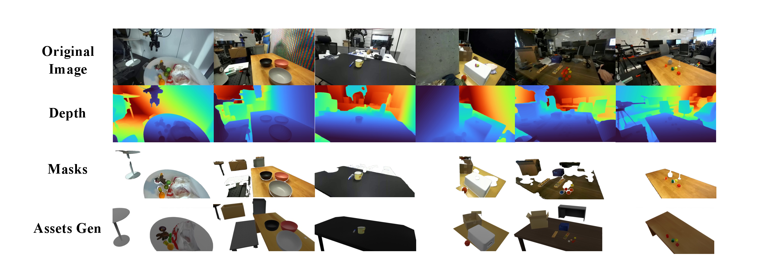
Our processing is automated after metadata parsing. For each retained scene folder, we extract one RGB frames (usually the first frame of one of the exterior camera) and query a VLM to produce object and support-surface captions, which are saved as
mask_prompt.txt. We then use Grounding DINO for text-conditioned localization, Florence-2 for referring-expression disambiguation when multiple detections match the same category, and SAM 3 for mask extraction [52], [65], [66].
This design avoids relying on a closed prompt list such as can/cup/mug/bowl/box/... because DROID includes long-tail household objects, tools, appliances, containers, and scene-specific distractors. The generated prompts, annotated views,
and merged masks are stored with each recovered scene as an auditable record of the automatic parsing stage.
After foreground mask extraction, we lift each retained object mask into a coarse 3D asset using SAM3D [25] and estimate an initial object pose from the selected RGB frame. We further predict a monocular depth map and reconstruct a masked object point cloud, which is aligned to the SAM3D asset using the initial pose. We then refine the object pose by performing point-to-plane ICP between mesh-sampled surface points and the observed depth point cloud, optimizing only rotation and translation while keeping the scale fixed. For the background, we segment the support surface and static scene region, complete the occluded background, and reconstruct a Gaussian-splatting representation of the scene background.
Based on runtime estimates over several hundred DROID-Sim scenes, the full automated pipeline from a single RGB frame to a foreground-background composited, simulation-ready scene takes approximately 12 to 25 minutes per scene, depending on the number of objects. On average, scenes with moderate complexity (around 5–10 objects) require approximately 17 minutes. The dominant costs come from background completion, Gaussian-splatting reconstruction, and the final simulation-readiness refinement.
10 Interactive Scene Construction GUI Tool↩︎
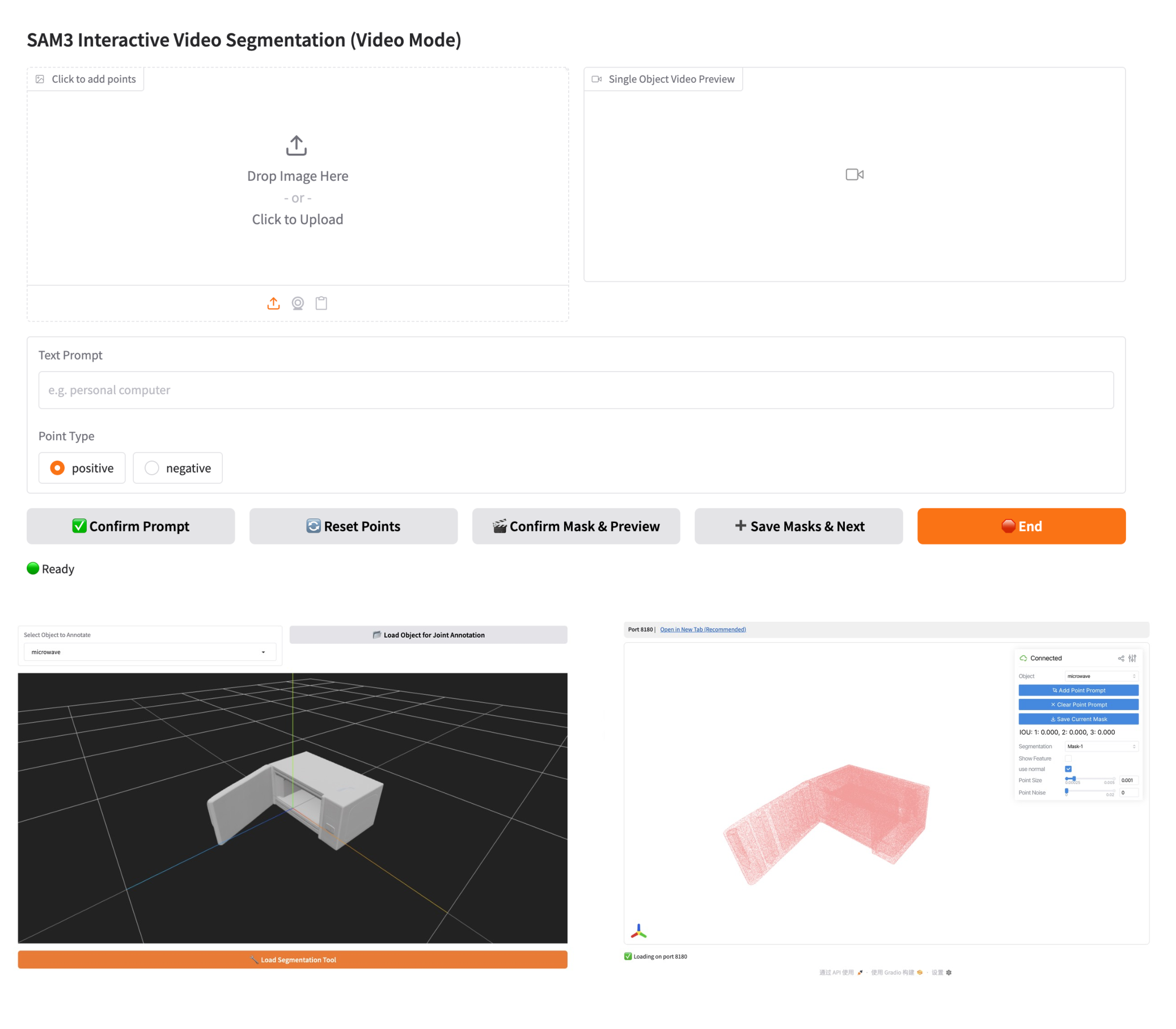
We implement an interactive GUI to simplify the construction of articulated 3D scenes from monocular images or videos. The interface is built with Gradio and integrates the complete workflow, including prompt-based mask initialization, click-based mask refinement, video mask propagation, 3D asset generation, scene-level GLB composition, and articulated-object annotation. Users first upload an image or video and specify the target object using a text prompt. The mask can then be refined through positive and negative clicks, allowing users to correct under-segmentation or over-segmentation before saving the object mask.
For video inputs, the system propagates the confirmed mask through the sequence and automatically selects a set of high-quality frames for 3D reconstruction. This multi-view mask selection improves the quality and completeness of the generated assets compared with relying on a single view. After all objects are segmented, the GUI invokes the SAM3D-based [25], [67] reconstruction pipeline to generate object-level GLB meshes and compose them into a scene-level asset. The user can then inspect the generated GLB files, select the object of interest, and enter the articulated-object interface, where the selected asset can be further segmented into parts and annotated with articulation information. This design avoids switching between separate scripts and visualization tools, making the overall scene construction process more reproducible and easier to operate.