Heat-Kernel Entropy Profiles and Geometric Effective Sample Size for Weighted Measures on Manifolds
July 07, 2026
Abstract
Weighted empirical measures on compact manifolds arise in importance sampling, particle approximations, posterior summaries, quadrature, and representation learning. Standard weight-only summaries, such as ordinary effective sample size, ignore the geometry of the support. We introduce heat-kernel entropy profiles, a multiscale summary that diffuses weighted atoms by intrinsic heat flow and tracks nonuniformity across scales. For order-two Rényi entropy, the profile is computable from pairwise heat-kernel overlaps and yields a geometric effective sample size that discounts nearby or duplicate particles while matching ordinary effective sample size for well-separated particles. We prove monotonicity, small- and large-scale asymptotics, deterministic-weight consistency, and a bounded-ratio self-normalized importance-sampling extension for compact manifolds without boundary. On spheres, the unlogged profile decomposes into spherical-harmonic energies that recover mean-direction, von Mises–Fisher-type, and Bingham-type summaries. Sphere-based experiments show that the profile reveals antipodal, girdle, multimodal, and duplicate-particle structure missed by weight-only and first-moment spherical summaries.
1 INTRODUCTION↩︎
Let \(\mathcal{M}\) be a compact Riemannian manifold and suppose a probability measure of interest is represented by weighted atoms, \[\widehat P_w=\sum_{i=1}^n w_i\delta_{x_i}, \quad x_i\in\mathcal{M},\; w_i\ge0,\; \sum_iw_i=1. \label{eq:weighted95measure}\tag{1}\] Such measures arise in quadrature, importance sampling, particle methods, posterior summaries, ensembles, and normalized representations. The natural question is how to summarize the uncertainty, diffuseness, or variability of 1 using both its weights and its geometry.
This problem matters because many standard diagnostics are label-based. The ordinary effective sample size (ESS), used in importance sampling and sequential Monte Carlo to monitor weight degeneracy [@kong_1994_SequentialImputationsBayesian; @liu_1998_SequentialMonteCarlo; @delmoral_2006_SequentialMonteCarlo], is \[\mathrm{ESS}(w)=\frac{1}{\sum_iw_i^2}.\] This is also the inverse-Simpson, or order-two Hill, effective number of the weights [@hill_1973_DiversityEvennessUnifying]. It diagnoses label-level weight concentration, but it is not a geometric property of the represented measure: splitting one atom into identical labels should not increase diffuseness, and equally weighted particles should count differently when close or far apart.
Geometric uncertainty is also scale-dependent. A weighted measure may look like many particles at fine resolution, a few clusters at medium resolution, and nearly uniform after enough smoothing. On spheres, first-moment summaries such as mean resultant length or fitted von Mises–Fisher (vMF) concentration [@fisher_1953_DispersionSphere; @mardia_2000_DirectionalStatistics; @banerjee_2005_ClusteringUnitHypersphere] can miss antipodal, girdle-like, or symmetric multimodal structure. This motivates our examples, while the method itself is manifold-level.
In response, we diffuse the weighted atoms by intrinsic heat flow and measure nonuniformity over diffusion time. For order-two Rényi entropy, the profile has an exact pairwise heat-kernel formula, so it is computed from Gram matrices rather than manifold integration. Normalizing the same overlaps gives a geometric effective sample size (gESS), an effective number of distinguishable atoms at each scale. Equivalently, the unlogged profile is a heat-kernel maximum mean discrepancy (MMD) to uniformity. Our contribution is its multiscale effective-volume and effective-number calibration, with small- and large-time interpretations.
The scope is intentionally specific. The theory is stated for compact, connected, boundaryless manifolds with normalized volume. Exact implementation requires either heat-kernel evaluations or controlled approximations. In experiments we use \(S^2\), where the heat kernel is explicit. The vMF and Bingham terminology used later is sphere-specific interpretation, not part of the general manifold definition.
1.0.0.1 Contributions.
We make five contributions. First, we introduce heat-kernel Rényi-2 entropy profiles for weighted empirical measures on compact manifolds and show that the order-two profile is computable from pairwise heat-kernel overlaps. Second, we derive a geometric effective sample size, or gESS, that discounts nearby and duplicate atoms while agreeing with ordinary effective sample size when atoms are well separated at the relevant scale. Third, we analyze the small-time regime, showing how local heat-kernel volume, curvature, duplicate coalescence, and two-atom merging determine the profile. Fourth, we prove a large-time spectral expansion and specialize it to spheres, where the first two nontrivial harmonic energies recover mean-direction and Bingham-type anisotropy summaries. Fifth, we establish stability and weighted-consistency results, including a bounded-ratio self-normalized importance-sampling case. Proofs and additional experiments are deferred to the appendix. Code to replicate examples is available at https://github.com/kisungyou/HeatKernelEntropyProfiles.
2 RELATED WORK↩︎
2.0.0.1 Weight-only and similarity-aware effective numbers.
Classical ESS diagnostics monitor weight degeneracy in importance sampling and sequential Monte Carlo, and discrepancy-based alternatives refine this goal [@martino_2017_EffectiveSampleSize]. Hill numbers and inverse-Simpson diversity give the same order-two effective-number interpretation [@hill_1973_DiversityEvennessUnifying], and Leinster–Cobbold diversity incorporates a user-chosen similarity matrix [@leinster_2012_MeasuringDiversityImportance]. Our gESS is an order-two similarity diversity, but the similarity is not arbitrary. It is the normalized heat-kernel overlap on the manifold. This choice is what gives the merge-invariance, scale limits, and heat-asymptotic interpretation proved below.
2.0.0.2 Heat smoothing, entropy, and kernel discrepancies.
Kernel density estimation on spheres and compact manifolds is well developed [@hall_1987_KernelDensityEstimation; @pelletier_2005_KernelDensityEstimation; @lebrigant_2019_ApproximationDensitiesRiemannian], and nearest-neighbor entropy estimators exist for hyperspherical data [@li_2011_KNearestNeighborBased]. These methods typically choose one smoothing scale to estimate one density or entropy. We instead treat the diffusion scale itself as the uncertainty resolution. For \(A_P(t)=\iint k_{2t}(x,y)\,\mathrm{d}P(x)\,\mathrm{d}P(y)\), the unlogged profile satisfies \(A_P(t)-1=\mathrm{MMD}_{k_{2t}}^2(P,\nu)\), connecting it to kernel mean embeddings [@sriperumbudur_2010_HilbertSpaceEmbeddings; @gretton_2012_KernelTwoSampleTest; @muandet_2017_KernelMeanEmbedding] and to Sobolev tests of uniformity on compact manifolds [@gine_1975_InvariantTestsUniformity; @garcia-portugues_2018_OverviewUniformityTests]. Unlike a raw MMD value, our outputs are calibrated as an effective occupied volume fraction and an effective number of geometrically distinguishable atoms across scales.
2.0.0.3 Spherical directional summaries.
On spheres, vMF and Bingham/Fisher–Bingham models provide classical first- and second-order summaries of directional structure [@kent_1982_FisherBinghamDistributionSphere; @mardia_2000_DirectionalStatistics]. We do not replace these parametric models in their intended unimodal or axial settings. Rather, it is shown that their basic moment energies appear as the first two nontrivial spectral components of the heat profile, while higher harmonic degrees capture structure that first- or second-order summaries do not separate.
3 HEAT ENTROPY PROFILES↩︎
Throughout, \(\mathcal{M}\) is a compact, connected, \(m\)-dimensional Riemannian manifold without boundary. Let \(\nu=\mathop{\mathrm{vol}}/\mathop{\mathrm{vol}}(\mathcal{M})\) be normalized Riemannian volume, so \(\nu(\mathcal{M})=1\) and the uniform density with respect to \(\nu\) is identically one. The notation \(\|\cdot\|\) is Euclidean for vectors, \(\|\cdot\|_F\) is Frobenius norm for matrices, and \(\|\cdot\|_q\) denotes the \(L^q(\nu)\) norm for functions. Let \(\Delta\) denote the Laplacian operator, so \(\partial_t u=\Delta u\) and the eigenvalues of \(-\Delta\) are nonnegative. Let \(k_t(x,y)\) be the heat kernel with respect to \(\nu\) [@rosenberg_1997_LaplacianRiemannianManifold; @grigoryan_2009_HeatKernelAnalysis]: \[\begin{align} \int_\mathcal{M}k_t(x,y)\,\mathrm{d}\nu(y)&=1,\\ k_{t+s}(x,y)&=\int_\mathcal{M}k_t(x,z)k_s(z,y)\,\mathrm{d}\nu(z). \end{align}\]
For a probability measure \(P\) on \(\mathcal{M}\), write \(H_tP\) for the heat-smoothed law. For every \(t>0\), \(H_tP\) has a smooth density \(p_t\) with respect to \(\nu\). Define \[\begin{align} D_{2,P}(t)&=\log\int_\mathcal{M}p_t(x)^2\,\mathrm{d}\nu(x),\\ U_{2,P}(t)&=\exp\{-D_{2,P}(t)\}. \end{align}\] Here \(D_{2,P}(t)\) is the order-two Rényi divergence of \(H_tP\) from the uniform reference measure \(\nu\), and \(U_{2,P}(t)\) is the corresponding effective occupied volume fraction.
For the weighted empirical measure 1 , the heat-smoothed density is \[\widehat p_t(y)=(H_t\widehat P_w)(y) =\sum_{i=1}^n w_i k_t(y,x_i). \label{eq:pt95def}\tag{2}\] The empirical heat entropy profile is obtained by evaluating the same functional at \(\widehat P_w\): \[\widehat D_2(t)=\log\int_\mathcal{M}\widehat p_t(y)^2\,\mathrm{d}\nu(y), \quad \widehat U_2(t)=\exp\{-\widehat D_2(t)\}.\] It is useful to write \[\widehat A_w(t)=\int_\mathcal{M}\widehat p_t(y)^2\,\mathrm{d}\nu(y),\] so that \(\widehat D_2(t)=\log \widehat A_w(t)\) and \(\widehat U_2(t)=\widehat A_w(t)^{-1}\).
The quantity \(U_{2,P}(t)\) is an effective occupied volume fraction. For an atomic input, \(U_{2,\widehat P_w}(t)\to0\) as \(t\downarrow0\) because the smoothed density becomes singular. The gESS introduced below divides out the local self-overlap of one heat kernel and therefore counts geometrically distinguishable atoms rather than volume.
Theorem 1 (Pairwise identity and monotonicity). For every \(t>0\), \[\widehat A_w(t) = \int_\mathcal{M}\widehat p_t(y)^2\,\mathrm{d}\nu(y) = \sum_{i,j=1}^n w_iw_jk_{2t}(x_i,x_j). \label{eq:pairwise95identity}\tag{3}\] Consequently, \[\widehat U_2(t) = \left[\sum_{i,j}w_iw_jk_{2t}(x_i,x_j)\right]^{-1}.\] Moreover, \(t\mapsto \widehat D_2(t)\) is nonincreasing and \(t\mapsto \widehat U_2(t)\) is nondecreasing. Finally, \[\lim_{t\to\infty}\widehat D_2(t)=0, \qquad \lim_{t\to\infty}\widehat U_2(t)=1.\]
The theorem says that intrinsic diffusion monotonically erases nonuniformity. The rate at which \(\widehat U_2(t)\) approaches one is the proposed uncertainty profile.
4 GEOMETRIC EFFECTIVE SAMPLE SIZE↩︎
The entropy profile measures effective volume. To obtain an effective number of distinguishable atoms, we normalize pairwise heat overlaps by the local self-overlap of each heat kernel.
Definition 1 (Geometric ESS). For \(t>0\), define \[s_t(x,y)=\frac{k_{2t}(x,y)}{\sqrt{k_{2t}(x,x)k_{2t}(y,y)}}\] and \[\mathrm{gESS}_w(t)=\left[\sum_{i,j}w_iw_js_t(x_i,x_j)\right]^{-1}.\]
On homogeneous manifolds such as spheres and compact Lie groups, \(k_{2t}(x,x)\) is constant. Then \[\mathrm{gESS}_w(t)=k_{2t}(x,x)\widehat U_2(t),\] so gESS is effective volume measured in units of the self-volume of one heat kernel. It is the order-two Hill/Leinster–Cobbold diversity for the heat-similarity matrix \(S_t=(s_t(x_i,x_j))_{ij}\) [@hill_1973_DiversityEvennessUnifying; @leinster_2012_MeasuringDiversityImportance].
Theorem 2 (Properties and limits of gESS). For every \(t>0\), \[0<s_t(x,y)\le1, \qquad s_t(x,x)=1.\] Consequently, \[1\le \mathrm{gESS}_w(t)\le \frac{1}{\sum_iw_i^2}=\mathrm{ESS}(w).\] If exact duplicate atoms are merged by summing their weights, \(\mathrm{gESS}_w(t)\) is unchanged. More generally, if the distinct support locations are \(z_1,\ldots,z_r\) with total masses \[\alpha_a=\sum_{i:x_i=z_a}w_i,\] then \[\lim_{t\downarrow0}\mathrm{gESS}_w(t)=\frac{1}{\sum_{a=1}^r\alpha_a^2}.\] In particular, if all \(x_i\) are distinct, the limit equals \(\mathrm{ESS}(w)\). Finally, \[\lim_{t\to\infty}\mathrm{gESS}_w(t)=1.\]
Theorem 2 formalizes the sense in which \(\mathrm{gESS}_w(t)\) upgrades ordinary ESS from a label-based quantity to a geometry-aware quantity. At fine scales, separated particles count separately, while at coarse scales all atoms become indistinguishable. The definition is also computationally modest as it requires only pairwise heat-kernel Gram matrices for a fixed grid of heat times. This makes the method comparable in cost to kernel discrepancy or MMD diagnostics, while returning an effective-number curve rather than only a discrepancy value. Algorithm 1 summarizes the computation, which is simply the pairwise identity in Theorem 1 followed by the normalization in Definition 1.
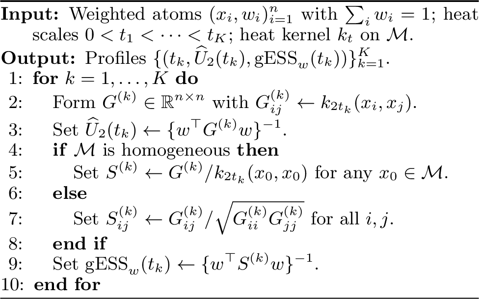
The two outputs have complementary interpretations. The \(\widehat U_2\) profile is a normalized volume, asking what fraction of the manifold is effectively occupied after diffusion. The \(\mathrm{gESS}_w\) profile is a normalized count that quantifies how many heat-kernel footprints are needed to represent the mass at that scale. The same pairwise overlaps therefore support both a density-level uncertainty summary and a particle-level degeneracy diagnostic. Figure 2 previews these two interpretations on the spherical examples studied later.
None
Figure 2: Preview of the proposed profiles on representative weighted measures on \(S^2\). The horizontal axis is angular resolution \(\alpha=\sqrt{8t}\) in degrees. Panel (a) shows the geometry-aware effective sample size, and panel (b) shows the effective occupied volume fraction..
5 ASYMPTOTIC INTERPRETATION↩︎
The next results explain what the proposed profiles measure at small and large diffusion scales. The small-time result describes the local regime in which each atom behaves like a small heat ball and nearby atoms begin to overlap. The large-time result describes the global regime in which heat flow has damped all but the lowest-frequency geometry. Together these results are the main reason the profile is interpretable rather than being just another kernel bandwidth curve.
5.1 Small-time behavior↩︎
Let \(V=\mathop{\mathrm{vol}}(\mathcal{M})\). For simplicity, collapse exact duplicates in \(\widehat P_w\) and write \[\widehat P_w=\sum_{a=1}^r\alpha_a\delta_{z_a}, \quad z_a\ne z_b\;(a\ne b),\; \sum_a\alpha_a=1,\] and define the local mass quantities \[S_\alpha=\sum_a\alpha_a^2, \quad C_\alpha=\sum_a\alpha_a^2 \mathop{\mathrm{Scal}}(z_a).\] The heat kernel with respect to normalized volume is \(V\) times the heat kernel with respect to Riemannian volume. The following fixed-configuration law is stated without displaying off-diagonal parametrix terms: for fixed distinct support points, those terms are exponentially smaller than every power of \(t\) and are therefore dominated by the diagonal heat expansion.
Theorem 3 (Fixed-configuration small-time law). As \(t\downarrow0\), \[\begin{align} \widehat A_w(t) &:=\sum_{a,b}\alpha_a\alpha_b k_{2t}(z_a,z_b) \notag\\ &=V(8\pi t)^{-m/2} \left[S_\alpha+\frac{t}{3}C_\alpha+O(t^2)+O(e^{-c/t})\right]. \label{eq:small95time95expansion} \end{align}\tag{4}\] for some \(c>0\) depending on the finite support. Consequently, \[\begin{align} \widehat D_2(t) &=\frac{m}{2}\log\frac{1}{8\pi t}+\log V+\log S_\alpha +\frac{t}{3}\frac{C_\alpha}{S_\alpha} \notag\\ &\quad+O(t^2)+O(e^{-c/t}),\\ \widehat U_2(t) &=\frac{(8\pi t)^{m/2}}{V}\frac{1}{S_\alpha} \left[1-\frac{t}{3}\frac{C_\alpha}{S_\alpha}+O(t^2)+O(e^{-c/t})\right]. \end{align}\] If all labels are distinct, then \(\alpha_a=w_a\).
Theorem 3 gives the asymptotic effective volume. To make the merging mechanism quantitative, the next proposition treats the local regime where pairwise distances are comparable to the diffusion radius.
Proposition 4 (Local two-atom merging law). Let \(P=a\delta_x+(1-a)\delta_y\) with \(0<a<1\) and \(r=d_g(x,y)\). Uniformly for \(r\) below a fixed injectivity radius and \(r^2=O(t)\) as \(t\downarrow0\), \[s_t(x,y)=\exp\left\{-\frac{r^2}{8t}\right\}\{1+O(t+r^2)\}. \label{eq:local95overlap}\qquad{(1)}\] Hence \[\begin{align} \mathrm{gESS}_P(t)^{-1} &=a^2+(1-a)^2 \notag\\ &\quad+2a(1-a)\exp\{-r^2/(8t)\}\notag\\ &\qquad\times\{1+O(t+r^2)\}. \label{eq:two95atom95gess} \end{align}\qquad{(2)}\]
Thus atoms at distance \(r\) merge when \(r^2\) is on the order of \(8t\). This motivates the angular-resolution convention used in the experiments. Specifically on spheres, we report the scale \(\alpha=\sqrt{8t}\) in radians. At distance \(r=\alpha\), the leading overlap is \(e^{-1}\).
5.2 Large-time spectral behavior↩︎
Let \(0=\lambda_0<\lambda_1\le\lambda_2\le\cdots\) be the Laplace–Beltrami eigenvalues and let \(\{\varphi_r\}_{r\ge0}\) be an orthonormal eigenbasis in \(L^2(\nu)\), with \(\varphi_0\equiv1\). Define weighted spectral coefficients \[\widehat a_r=\sum_iw_i\varphi_r(x_i),\qquad r\ge1.\] The heat-kernel spectral representation [@rosenberg_1997_LaplacianRiemannianManifold; @grigoryan_2009_HeatKernelAnalysis] gives the following results.
Theorem 5 (Spectral expansion). For every \(t>0\), \[\widehat p_t-1=\sum_{r\ge1}e^{-\lambda_rt}\widehat a_r\varphi_r, \label{eq:pt95spectral}\tag{5}\] and \[\widehat D_2(t)=\log\left(1+\sum_{r\ge1}e^{-2\lambda_rt}\widehat a_r^2\right). \label{eq:D295spectral}\tag{6}\] Equivalently, \[\begin{align} \widehat A_w(t)-1 &=\frac{1}{\widehat U_2(t)}-1 \notag\\ &=\sum_{r\ge1}e^{-2\lambda_rt}\widehat a_r^2. \label{eq:Aminus95spectral} \end{align}\tag{7}\] Consequently, as \(t\to\infty\), if \(\lambda_+\) is the next distinct eigenvalue after \(\lambda_1\), then \[\begin{align} \widehat D_2(t) &=e^{-2\lambda_1t}\sum_{\lambda_r=\lambda_1}\widehat a_r^2 \notag\\ &\quad+O\left(e^{-2\lambda_+t}+e^{-4\lambda_1t}\right), \end{align}\]
The exact expansion 7 is often more interpretable than the logged entropy because it has no logarithmic cross terms. Large-scale uncertainty is controlled by the lowest nonzero eigenmodes, i.e., by the structures that survive longest under diffusion.
6 SPHERICAL SPECIALIZATION: vMF AND BINGHAM STRUCTURE↩︎
We now leave the general compact-manifold setting and specialize to the sphere \(S^{p-1}\) of dimension \(m=p-1\). This section is interpretive: on spheres, the first few Laplace–Beltrami eigenspaces have familiar meanings in directional statistics. Degree one corresponds to a preferred direction, degree two to axial or elliptical departures from uniformity, and higher degrees to multimodality and finer angular structure. Let \(\nu\) be normalized surface measure. The Laplace–Beltrami eigenvalues are \[\lambda_\ell=\ell(\ell+p-2),\qquad \ell=0,1,2,\ldots,\] with eigenspaces given by degree-\(\ell\) spherical harmonics. We write \(\widehat a_{\ell j}=\sum_iw_iY_{\ell j}(x_i)\) for coefficients in an orthonormal basis of the degree-\(\ell\) eigenspace. This is the double-index version of Theorem 5: sums over all single indices \(r\) with \(\lambda_r=\lambda_\ell\) become \(\sum_j\widehat a_{\ell j}^2\).
Let \[\bar x_w=\sum_iw_ix_i, \quad Q_w=\sum_iw_ix_ix_i^\top.\] The degree-1 spectral energy is \[B_1:=\sum_j\widehat a_{1j}^2=p\|\bar x_w\|^2, \label{eq:B1}\tag{8}\] and the degree-2 spectral energy is \[B_2:=\sum_j\widehat a_{2j}^2=\frac{p(p+2)}{2}\left\|Q_w-\frac{I_p}{p}\right\|_F^2. \label{eq:B2}\tag{9}\]
Corollary 1 (Spherical power expansion). On \(S^{p-1}\), \[\begin{align} \widehat A_w(t)-1 &=\frac{1}{\widehat U_2(t)}-1 \notag\\ &=\sum_{\ell\ge1}e^{-2\ell(\ell+p-2)t}\sum_j\widehat a_{\ell j}^2 \notag\\ &=e^{-2(p-1)t}B_1+e^{-4pt}B_2+ \sum_{\ell\ge3}e^{-2\ell(\ell+p-2)t}B_\ell, \end{align}\] where \(B_\ell=\sum_j\widehat a_{\ell j}^2\). Moreover, \[\widehat D_2(t)=\log\{1+\widehat A_w(t)-1\}.\] Thus, when \(B_1\ne0\), the logged entropy contains the cross term \[-\frac{1}{2}e^{-4(p-1)t}B_1^2\] before the displayed degree-2 term. If \(B_1=0\), the \(B_2\) term is the leading logged contribution whenever degree two is nonzero.
The term \(B_1\) is exactly the squared weighted mean resultant length up to the factor \(p\), i.e., the first-moment spherical structure captured by the Rayleigh statistic and vMF fitting. The term \(B_2\) captures spherical axial, antipodal, and elliptical structure, analogous to Bingham or Fisher–Bingham modeling [@kent_1982_FisherBinghamDistributionSphere]. Higher degrees capture multimodality and finer angular structure on the sphere. Corollary 1 makes the safest interpretation precise. The vMF and Bingham energies are sphere-specific interpretations of the first two coefficients of the unlogged heat-power profile \(\widehat A_w(t)-1\), while the logarithm introduces lower-degree self-interaction terms.
7 WEIGHTED CONSISTENCY↩︎
The previous sections treat the profile as a deterministic functional of the weighted measure. In applications, the weighted atoms may themselves approximate a target distribution. The next result gives a basic stability guarantee: the closer the weighted empirical measure is to the target, the closer the whole heat-power curve should be on any scale interval bounded away from zero. Existence of the lower cutoff is unavoidable, because heat kernels become increasingly singular as \(t\) approaches zero. Let \[\begin{align} A_P(t)&=\iint k_{2t}(x,y)\,\mathrm{d}P(x)\,\mathrm{d}P(y), \\ \widehat A_w(t)&=\sum_{i,j}w_iw_jk_{2t}(x_i,x_j), \end{align}\] and \[D_{2,P}(t)=\log A_P(t).\]
Assumption 1 (Regular heat-kernel class). Fix \(0<t_0<T<\infty\) and set \(g_t(x,y)=k_{2t}(x,y)\). The class \(\mathcal{G}=\{g_t:t\in[t_0,T]\}\) is uniformly bounded and uniformly Lipschitz in \(x,y,t\), and for some constants \(C_0,C_1\), \[N(\varepsilon,\mathcal{G},\|\cdot\|_\infty)\le C_0\varepsilon^{-1}, \qquad 0<\varepsilon<C_1.\]
This assumption is used only for the stochastic uniform-in-\(t\) rate. On a compact boundaryless manifold, it follows from smoothness of \(k_t\) for \(t\ge t_0\) and the constants deteriorate as \(t_0\downarrow0\). Hence, we state the theorem on scale intervals bounded away from zero.
Theorem 6 (Stability and weighted convergence). Fix \(0<t_0<T<\infty\). There is a constant \(C=C(t_0,T,\mathcal{M})\) such that for any two probability measures \(P,Q\) on \(\mathcal{M}\), \[\sup_{t\in[t_0,T]} |A_P(t)-A_Q(t)| \le C W_1(P,Q), \label{eq:W195stability}\tag{10}\] where \(W_1\) is the geodesic Wasserstein-1 distance. Consequently, if \(\widehat P_w\to P\) in \(W_1\), then \[\sup_{t\in[t_0,T]} |\widehat D_2(t)-D_{2,P}(t)|\to0.\] Assume in addition Assumption 1. If \(X_1,\ldots,X_n\overset{iid}{\sim}P\) and deterministic weights satisfy \(S_n:=\sum_iw_i^2\to0\), then \[\sup_{t\in[t_0,T]} |\widehat A_w(t)-A_P(t)| =O_p\left(\sqrt{S_n\log(1/S_n)}\right), \label{eq:weighted95rate}\tag{11}\] and the same rate holds for \(\widehat D_2(t)\).
Finally, let \(X_i\overset{iid}{\sim}Q\), let \(P\) have bounded density ratio \(\rho=\,\mathrm{d}P/\,\mathrm{d}Q\) with \(0\le\rho\le M\) and \(\mathbb{E}_Q\rho=1\), and set self-normalized importance weights \(w_i=\rho(X_i)/\sum_j\rho(X_j)\). Then \[\sup_{t\in[t_0,T]} |\widehat A_w(t)-A_P(t)|=O_p\left(\sqrt{\frac{\log n}{n}}\right),\] with the same rate for \(\widehat D_2(t)\).
The deterministic-weight rate is worst-case. If \(P=\nu\), the linear term in the Hoeffding decomposition vanishes, and the leading stochastic term improves to the degenerate order \(S_n\) up to logarithmic factors. The constants necessarily deteriorate as \(t_0\downarrow0\), and heat-kernel suprema and derivatives scale like powers of \(t_0^{-1}\). This reflects a fine-scale interpretability versus fine-scale estimability trade-off.
8 EXPERIMENTS↩︎
The theoretical construction and consistency results above are manifold-level statements. The experiments below focus on \(S^2\) because its heat kernel is explicit and because the failure modes of first-moment directional summaries are easy to visualize. The synthetic examples are stress tests that include configurations where weight-only ESS and first-moment spherical summaries are expected to fail, as visualized in Figure 3.
None
Figure 3: Mollweide projections of the five synthetic \(S^2\) configurations. These visualizations make the failure modes of ordinary ESS and first-moment summaries explicit: antipodal, girdle, and four-mode structures can have small resultant length but remain highly nonuniform at relevant scales..
The reported synthetic values correspond to the constructions described in Appendix 11. All quantities are computed by the routine in Section 4. The only sphere-specific step is evaluating the heat Gram matrix. The heat kernel is \[k_t(x,y)=\sum_{\ell=0}^{\infty}(2\ell+1)e^{-\ell(\ell+1)t}P_\ell(x^\top y), \label{eq:s295heat}\tag{12}\] where \(P_\ell\) is the Legendre polynomial. For a fixed weighted cloud, we compute the harmonic energies \[B_\ell=(2\ell+1)\sum_{i,j}w_iw_jP_\ell(x_i^\top x_j)\] once and evaluate \[\widehat A_w(t)=\sum_{\ell\ge0}e^{-2\ell(\ell+1)t}B_\ell.\] As a similarity-sensitive baseline, we use a Leinster–Cobbold-style diversity with geodesic Gaussian similarity, \[D_{\rm LC}^{(\alpha)}=\left[\sum_{i,j}w_iw_j\exp\{-(d_g(x_i,x_j)/\alpha)^2\}\right]^{-1}.\] It matches the \(e^{-1}\) overlap convention at \(d_g=\alpha\) but is not derived from the manifold heat semigroup. We also report the ordinary \(\ell_2\) ESS and, in the real-data table, the entropy/perplexity ESS \(\mathrm{ESS}_H=\exp\{-\sum_iw_i\log w_i\}\), a weight-only discrepancy/entropy baseline discussed in ESS surveys [@martino_2017_EffectiveSampleSize]. The heat-kernel MMD curve is exactly \(\widehat A_w(t)-1\), as noted in Section 2. Figure 4 uses this unlogged curve to validate the small- and large-scale asymptotics.
None
Figure 4: Two-regime validation for a unimodal vMF cloud on \(S^2\). Panel (a) compares \(\widehat A_w(t)\) to the leading small-time pairwise heat-overlap approximation. Panel (b) compares \(\widehat A_w(t)-1\) to the low-frequency approximation. The unlogged power is used because it is the cross-term-free object in the spherical expansion..
8.0.0.1 Synthetic configurations.
The synthetic examples are designed to isolate distinct failure modes. The unimodal cloud is the case where all summaries should agree. The antipodal and girdle examples have nearly vanishing first moment but strong nonuniform structure. The four-mode example tests whether the profile behaves like a scale-dependent mode count. The duplicate example tests the atom-splitting invariance that ordinary ESS lacks. We compare five equal-weight configurations with \(n=300\): a concentrated vMF cloud, an antipodal mixture, an equatorial girdle, four separated modes, and exact duplicates at 30 quasi-uniform locations. Table 1 reports scalar summaries at selected scales. Ordinary ESS is 300 in every row. The resultant length \(R\) fails on symmetric nonuniform examples, \(B_2\) captures axial structure for antipodal and girdle examples, and gESS gives the scale-dependent count of distinguishable atoms. The duplicate example has 300 labels but only 30 locations, and gESS at \(15^\circ\) is approximately 30, as required by merge-invariance.
| Example | \(R\) | \(B_2\) | ESS | \(\gess(15^\circ)\) | \(D_{\rm LC}^{(15)}\) | \(\gess(45^\circ)\) |
|---|---|---|---|---|---|---|
| Unimodal vMF | 0.993 | 4.79 | 300 | 1.4 | 1.4 | 1.0 |
| Antipodal | 0.006 | 4.78 | 300 | 2.9 | 2.9 | 2.1 |
| Girdle | 0.029 | 1.24 | 300 | 13.3 | 13.4 | 4.4 |
| Four modes | 0.007 | 0.00 | 300 | 5.5 | 5.5 | 4.1 |
| Duplicates | 0.005 | 0.00 | 300 | 29.7 | 29.7 | 6.8 |
8.0.0.2 Real-data embedding illustration.
As a lightweight real-data example, we use the handwritten digits dataset1 available via the scikit-learn package [@pedregosa_2011_ScikitlearnMachineLearning]. We standardize the \(8\times8\) images, project to three principal components, and normalize onto \(S^2\). The substantive question is whether a geometry-aware summary changes the interpretation of a normalized embedding when the same points are reweighted or restricted to a subset. Table 2 shows that nonuniform reliability-style weights reduce both ordinary ESS and geometric occupancy, while the 0-vs-1 subset has a different directional structure from the full ten-class cloud.
| Data | \(n\) | \(R\) | \(B_2\) | ESS | \(\ess_H\) | \(\gess(15^\circ)\) | \(D_{\rm LC}^{(15)}\) |
|---|---|---|---|---|---|---|---|
| Digits all | 300 | 0.152 | 0.07 | 300 | 300 | 36.7 | 36.8 |
| Digits weighted | 300 | 0.649 | 0.53 | 123 | 156 | 15.4 | 15.5 |
| Digits 0/1 | 60 | 0.540 | 0.81 | 60 | 60 | 9.8 | 9.9 |
9 DISCUSSION↩︎
Heat-kernel entropy profiles provide an intrinsic way to quantify uncertainty of weighted empirical measures on compact manifolds. The order-two Rényi case is especially useful because it is computable through pairwise heat overlaps, yields a geometry-aware ESS, and has clear small- and large-time interpretations without relying on spherical parametrization. The small-time expansion shows when ordinary ESS is recovered: only at resolutions where particles are geometrically separated. The large-time expansion shows which low-frequency structures survive diffusion.
The scope of the paper is deliberate. The theory assumes compact, connected, boundaryless manifolds and normalized Riemannian volume. The profile \(\widehat U_2(t)\) is monotone by Theorem 1, but \(\mathrm{gESS}_w(t)\) need not be monotone on a nonhomogeneous manifold because the diagonal heat-kernel normalization varies with location. Exact computation also requires heat-kernel evaluations. On spheres and compact Lie groups, harmonic expansions are natural. On general manifolds, one may use spectral truncation, graph Laplacians [@chung_1997_SpectralGraphTheory], diffusion maps [@coifman_2006_DiffusionMaps], or numerical heat solvers.
The statistical results also have a scale boundary. Small scales are the most informative about fine structure but the least stable statistically, because heat-kernel suprema and derivatives grow as \(t\downarrow0\). The consistency result is therefore stated on intervals \([t_0,T]\) with \(t_0>0\). The experiments are descriptive profile demonstrations rather than calibrated inferential comparisons, since they do not provide confidence bands. Future work includes inference for whole profiles, heavy-tailed self-normalized importance weights beyond the bounded-ratio theorem, extensions to noncompact manifolds through reference measures, and joint use with maximum-entropy hierarchies for model-based uncertainty decomposition.
10 PROOFS↩︎
10.1 Proof of Theorem 1↩︎
By bilinearity and the definition of \(\widehat p_t\), \[\int \widehat p_t(y)^2\,\mathrm{d}\nu(y) =\sum_{i,j}w_iw_j\int k_t(y,x_i)k_t(y,x_j)\,\mathrm{d}\nu(y).\] The heat kernel is symmetric and satisfies the semigroup identity, hence the integral equals \(k_{2t}(x_i,x_j)\). This proves 3 .
For monotonicity, \(\widehat p_t\) solves \(\partial_t\widehat p_t=\Delta\widehat p_t\), with the convention that the spectrum of \(-\Delta\) is nonnegative. Since \(\mathcal{M}\) is compact without boundary, \[\begin{align} \frac{d}{dt}\int \widehat p_t^2\,\mathrm{d}\nu &=2\int \widehat p_t\Delta\widehat p_t\,\mathrm{d}\nu =-2\int\|\nabla\widehat p_t\|^2\,\mathrm{d}\nu\le0. \end{align}\] Therefore \(\widehat D_2(t)=\log\|\widehat p_t\|_2^2\) is nonincreasing and \(\widehat U_2(t)\) is nondecreasing. Since \(\mathcal{M}\) is compact and connected, heat flow converges to the constant density \(1\) in \(L^2(\nu)\), so \(\|\widehat p_t\|_2^2\to1\).
10.2 Proof of Theorem 2↩︎
The semigroup identity gives \[\begin{align} k_{2t}(x,y)&=\int k_t(x,z)k_t(y,z)\,\mathrm{d}\nu(z)\\ &=\left\langle k_t(x,\cdot),k_t(y,\cdot)\right\rangle_{L^2(\nu)}. \end{align}\] The heat kernel is strictly positive on a connected compact manifold for \(t>0\), so \(s_t(x,y)>0\). By Cauchy–Schwarz inequality, \[k_{2t}(x,y)^2\le k_{2t}(x,x)k_{2t}(y,y),\] which proves \(s_t(x,y)\le1\) and \(s_t(x,x)=1\).
Since \(s_t(x_i,x_j)\le1\) and \(\sum_{i,j}w_iw_j=1\), \[\sum_{i,j}w_iw_js_t(x_i,x_j)\le1,\] so \(\mathrm{gESS}_w(t)\ge1\). Since \(s_t(x_i,x_i)=1\) and off-diagonal terms are nonnegative, \[\sum_{i,j}w_iw_js_t(x_i,x_j)\ge\sum_iw_i^2,\] so \(\mathrm{gESS}_w(t)\le1/\sum_iw_i^2\).
If duplicate atoms are merged, the double sum is unchanged because all terms involving the duplicate location have the same similarity value. If distinct support points are \(z_a\) with masses \(\alpha_a\), then the denominator can be written as \[\sum_{a,b}\alpha_a\alpha_bs_t(z_a,z_b).\] As \(t\downarrow0\), \(s_t(z_a,z_a)=1\) and \(s_t(z_a,z_b)\to0\) for \(a\ne b\): Gaussian upper bounds for \(k_t(z_a,z_b)\) combined with diagonal lower bounds imply this uniformly away from the diagonal [@grigoryan_2009_HeatKernelAnalysis]. Thus the denominator converges to \(\sum_a\alpha_a^2\). As \(t\to\infty\), the spectral expansion and the spectral gap imply \(k_{2t}(x,y)\to1\) uniformly, so \(s_t(x,y)\to1\) and the denominator converges to \(1\).
10.3 Proof of Theorem 3 and Proposition 4↩︎
Let \(K_t\) denote the heat kernel with respect to Riemannian volume. Since \(\nu=\mathop{\mathrm{vol}}/V\), the heat kernel with respect to \(\nu\) is \(k_t=VK_t\). The diagonal Minakshisundaram–Pleijel expansion [@rosenberg_1997_LaplacianRiemannianManifold; @grigoryan_2009_HeatKernelAnalysis] gives \[K_s(x,x)=(4\pi s)^{-m/2}\left[1+\frac{s}{6}\mathop{\mathrm{Scal}}(x)+O(s^2)\right].\] With \(s=2t\), \[k_{2t}(z_a,z_a)=V(8\pi t)^{-m/2}\left[1+\frac{t}{3}\mathop{\mathrm{Scal}}(z_a)+O(t^2)\right].\] Since the coalesced support points \(z_a\) are finite and distinct, their minimum nonzero distance is positive. Heat-kernel Gaussian upper bounds [@grigoryan_2009_HeatKernelAnalysis] imply that the total off-diagonal contribution is \(V(8\pi t)^{-m/2}O(e^{-c/t})\) for some \(c>0\). Summing the diagonal terms gives 4 . The expansions for \(\widehat D_2\) and \(\widehat U_2\) follow by applying \(\log(S_\alpha+\epsilon)\) and \((S_\alpha+\epsilon)^{-1}\) Taylor expansions with \(\epsilon=(t/3)C_\alpha+O(t^2)+O(e^{-c/t})\).
For Proposition 4, use the near-diagonal heat-kernel parametrix uniformly in a normal neighborhood: \[K_s(x,y)=(4\pi s)^{-m/2}\exp\left\{-\frac{d_g(x,y)^2}{4s}\right\} \{u_0(x,y)+O(s)\},\] where \(u_0(x,y)\) is the square root of the inverse Jacobian determinant of the exponential map and \(u_0(x,y)=1+O(d_g(x,y)^2)\). Combining this with the diagonal expansion in the denominator of \(s_t(x,y)\) and taking \(s=2t\) yields ?? . Substituting into the exact denominator \(a^2+(1-a)^2+2a(1-a)s_t(x,y)\) proves ?? .
10.4 Proof of Theorem 5↩︎
The heat kernel has the spectral representation \[k_t(x,y)=\sum_{r\ge0}e^{-\lambda_rt}\varphi_r(x)\varphi_r(y),\] where \(\varphi_0\equiv1\). Substituting this into 2 gives \[\widehat p_t(y)=1+\sum_{r\ge1}e^{-\lambda_rt}\left(\sum_iw_i\varphi_r(x_i)\right)\varphi_r(y),\] which is 5 . Orthogonality implies \[\int\widehat p_t^2\,\mathrm{d}\nu=1+\sum_{r\ge1}e^{-2\lambda_rt}\widehat a_r^2,\] which proves 6 and 7 . The large-time expansion follows from \(\log(1+z)=z+O(z^2)\), separating the lowest nonzero eigenspace from the rest.
10.5 Proof of Corollary 1↩︎
For \(S^{p-1}\) with normalized surface measure, the coordinate functions satisfy \[\int x_ax_b\,\mathrm{d}\nu(x)=\frac{\delta_{ab}}{p}.\] Thus \(\sqrt p\,x_a\), \(a=1,\ldots,p\), form an orthonormal basis of the degree-1 eigenspace. The degree-1 energy is therefore \[\sum_{a=1}^p\left(\sum_iw_i\sqrt p\,x_{ia}\right)^2=p\left\|\sum_iw_ix_i\right\|^2.\]
For degree 2, let \(A\) and \(B\) be symmetric traceless matrices. The fourth-moment identity on the sphere gives \[\int (x^\top A x)(x^\top Bx)\,\mathrm{d}\nu(x) =\frac{2\mathop{\mathrm{tr}}(AB)}{p(p+2)}.\] Hence \(A\mapsto \sqrt{p(p+2)/2}\,x^\top A x\) is an isometry from the space of symmetric traceless matrices with Frobenius inner product into the degree-2 harmonic subspace. It is onto because both spaces have dimension \(p(p+1)/2-1\). Since \(Q_w-I_p/p\) is the traceless part of \(Q_w\), the degree-2 energy is \[\frac{p(p+2)}{2}\left\|Q_w-\frac{I_p}{p}\right\|_F^2.\] This proves 8 and 9 .
10.6 Proof of Theorem 6↩︎
We first prove deterministic stability. For fixed \(t\in[t_0,T]\), define \[f_{P,t}(x)=\int k_{2t}(x,y)\,\mathrm{d}P(y).\] The compactness of \(\mathcal{M}\) and \(t\ge t_0>0\) imply that \(k_{2t}\) and its first spatial derivatives are uniformly bounded over \((x,y,t)\in\mathcal{M}^2\times[t_0,T]\). Thus \(f_{P,t}\) is uniformly Lipschitz with constant at most \(L=L(t_0,T,\mathcal{M})\). For two probability measures \(P,Q\), \[\begin{align} A_P(t)-A_Q(t) &=\iint k_{2t}(x,y)\,\mathrm{d}(P-Q)(x)\,\mathrm{d}P(y) \\ &\quad+\iint k_{2t}(x,y)\,\mathrm{d}Q(x)\,\mathrm{d}(P-Q)(y). \end{align}\] By Kantorovich–Rubinstein duality, each term is bounded by \(L W_1(P,Q)\). This proves 10 with \(C=2L\), uniformly in \(t\in[t_0,T]\). Since \(A_P(t)=\|p_t\|_2^2\ge1\), the logarithm is one-Lipschitz on the relevant range.
For the random weighted rate, set \(g_t(x,y)=k_{2t}(x,y)\) and write \(S_n=\sum_iw_i^2\). Under Assumption 1, \(\mathcal{G}\) is bounded by \(B\) and Lipschitz in \(t\) by \(L_t\). Use the weighted Hoeffding decomposition \[\begin{align} \widehat A_w(t)-A_P(t) &=2\sum_iw_i h_{1,t}(X_i) +\sum_{i\ne j}w_iw_j h_{2,t}(X_i,X_j)\notag\\ &\quad+\sum_iw_i^2\{g_t(X_i,X_i)-A_P(t)-2h_{1,t}(X_i)\}, \end{align}\] where \(h_{1,t}(x)=\mathbb{E}g_t(x,X)-A_P(t)\) and \(h_{2,t}(x,y)=g_t(x,y)-A_P(t)-h_{1,t}(x)-h_{1,t}(y)\) is canonical: \(\mathbb{E}[h_{2,t}(x,X)]=0\).
The diagonal term is bounded by \(C S_n\) uniformly. For the linear term, choose an \(\varepsilon\)-net of \([t_0,T]\) of size at most \(C/\varepsilon\). At a fixed net point, Bernstein’s inequality for the weighted sum of bounded centered variables gives \[\begin{align} &\Pr\left(\left|\sum_iw_i h_{1,t}(X_i)\right|>u\right) \notag\\ &\quad\le 2\exp\left[-c\min\left\{\frac{u^2}{B^2S_n},\frac{u}{B\max_iw_i}\right\}\right]. \end{align}\] Since \(\max_iw_i\le S_n^{1/2}\), taking \(u=C\sqrt{S_n\log(1/S_n)}\) and \(\varepsilon\asymp u/L_t\) makes the union bound over the net summable; Lipschitz interpolation gives \[\sup_{t\in[t_0,T]}\left|\sum_iw_i h_{1,t}(X_i)\right| =O_p\{\sqrt{S_n\log(1/S_n)}\}.\]
For the degenerate term, the same net is used, but the process is quadratic. Decoupling for canonical \(U\)-processes [@arcones_1993_LimitTheorems-dollar-U-dollar-Processes; @delapena_1999_Decoupling] reduces the supremum to a decoupled Rademacher chaos. For each fixed net point, the variance proxy is bounded by \(C\sum_{i\ne j}w_i^2w_j^2\le C S_n^2\) and the envelope by \(C\max_{i\ne j}w_iw_j\le C S_n\). A degenerate-U-statistic Bernstein inequality therefore yields \[\begin{align} &\Pr\left(\left|\sum_{i\ne j}w_iw_j h_{2,t}(X_i,X_j)\right|>u\right) \notag\\ &\quad\le 2\exp\left[-c\min\left\{\frac{u^2}{S_n^2},\frac{u}{S_n}\right\}\right]. \end{align}\] With \(u=C S_n\log(1/S_n)\), the net union bound and Lipschitz interpolation give \[\sup_t\left|\sum_{i\ne j}w_iw_j h_{2,t}(X_i,X_j)\right| =O_p\{S_n\log(1/S_n)\}.\] This is lower order than the displayed worst-case linear rate. Combining the three terms proves 11 .
For self-normalized importance sampling, write \(Z_n=n^{-1}\sum_i\rho(X_i)\) and \[\widehat A_w(t)=\frac{n^{-2}\sum_{i,j}\rho(X_i)\rho(X_j)g_t(X_i,X_j)}{Z_n^2}.\]
The numerator is an ordinary V-statistic for the bounded kernel \(\rho(x)\rho(y)g_t(x,y)\) under \(Q\). Its off-diagonal expectation is \(A_P(t)\), while the diagonal contributes only \(O(n^{-1})\) uniformly over \(t\in[t_0,T]\) because \(\rho\) and \(g_t\) are bounded. The equal-weight version of the preceding argument gives a uniform \(O_p(\sqrt{\log n/n})\) rate. Also \(Z_n=1+O_p(n^{-1/2})\) by boundedness of \(\rho\), so the denominator perturbation is of the same or smaller order. This proves the self-normalized statement.
11 ADDITIONAL EXPERIMENTS AND REPRODUCIBILITY↩︎
This appendix gives the experimental details needed to reproduce the main figures and tables, and it reports additional experiments that stress the proposed profiles beyond the point summaries in the main text. The additional experiments address four questions: whether the profiles are stable across replications, how sensitive the spherical heat-kernel computation is to spectral truncation, how ordinary effective sample size and gESS behave in a self-normalized importance-sampling problem, and what the complete real-data profiles look like beyond the scalar summaries in Table 2.
11.0.0.1 Synthetic configurations on \(S^2\).
All five synthetic examples in Table 1 use equal weights and \(n=300\) labeled atoms. The unimodal example is sampled from a vMF distribution on \(S^2\) with mean direction \(e_3=(0,0,1)^\top\) and concentration \(\kappa=140\). The antipodal example contains 150 samples from the same vMF distribution and 150 samples from the antipodal component with mean direction \(-e_3\) and the same concentration \(\kappa=140\). The girdle example is generated by drawing an equatorial angle \(\theta\sim\mathrm{Unif}(0,2\pi)\) and a vertical perturbation \(z\sim N(0,0.035^2)\), then normalizing \[(\cos\theta,\sin\theta,z)^\top\] to unit length. The four-mode example uses the four tetrahedral directions \[\frac{(1,1,1)}{\sqrt3},\quad \frac{(1,-1,-1)}{\sqrt3},\quad \frac{(-1,1,-1)}{\sqrt3},\quad \frac{(-1,-1,1)}{\sqrt3},\] with 75 vMF samples from each center and concentration \(\kappa=140\). The duplicate example first constructs 30 quasi-uniform Fibonacci-sphere locations and then repeats each location ten times. Thus it has 300 labeled atoms but only 30 distinct support points. This example is included to test exact atom-splitting invariance.
11.0.0.2 Angular scale, heat-kernel computation, and truncation.
On \(S^2\), we report diffusion time through the angular resolution \[\alpha=\sqrt{8t},\] given in degrees after multiplying radians by \(180/\pi\). This convention is motivated by the small-time overlap law \(\exp\{-d_g(x,y)^2/(8t)\}\): two atoms at distance \(d_g(x,y)=\alpha\) have leading heat overlap \(e^{-1}\). The heat kernel is evaluated by the spectral series \[k_t(x,y)=\sum_{\ell=0}^{\infty}(2\ell+1)e^{-\ell(\ell+1)t} P_\ell(x^\top y).\] For the main figures and tables we truncate the series at \(L=140\) over the reported scale range. When evaluating \(k_{2t}\), the diagonal truncation tail is bounded by \[\sum_{\ell>L}(2\ell+1)e^{-2t\ell(\ell+1)}.\] Practitioners should increase \(L\) on the order of \(t^{-1/2}\) when probing finer diffusion scales. Once heat-kernel values are available, the Gram-matrix cost for evaluating \(K\) heat scales is \(O(n^2K)\).
11.0.0.3 Replicated synthetic profiles.
Figure 5 repeats variants of the synthetic constructions over 30 independent replications, using \(n=180\) points per replication. To make between-replication variation visible, these replicated runs use concentration \(\kappa=100\) for vMF components, an equatorial perturbation standard deviation of \(0.045\) for the girdle, and 20 distinct Fibonacci-sphere locations repeated nine times for the duplicate example. Curves show medians and shaded interquartile ranges.
None
Figure 5: Replicated synthetic profiles on \(S^2\). Each curve is the median over 30 replications, and the shaded region is the interquartile range. Left: geometry-aware effective sample size, which counts distinguishable atoms or clusters. Right: effective occupied volume fraction, which increases as heat flow removes nonuniformity. The plot checks that the qualitative profile shapes are stable across replications..
11.0.0.4 Spectral truncation sensitivity.
Figure 6 varies the truncation level \(L_{\max}\) in the \(S^2\) heat-kernel expansion. The reference value uses \(L_{\max}=360\), and the figure reports relative error in \(\widehat A_w(t)\) for a four-mode cloud. Fine angular scales require more terms, consistent with the rule of thumb \(L_{\max}\) on the order of \(t^{-1/2}\). The main-paper truncation level is adequate for the scales reported there, but the figure also shows that very fine scales are both statistically and numerically more fragile.
None
Figure 6: Sensitivity of the \(S^2\) heat-profile computation to harmonic truncation. The plot shows relative error in \(\widehat A_w(t)\) against a longer-series reference as a function of angular resolution. Smaller angular scales require more spherical-harmonic terms because high frequencies have not yet been damped by heat flow. Errors below \(10^{-16}\) are clipped for log-scale visualization..
11.0.0.5 Self-normalized importance-sampling diagnostic.
Figure 7 simulates self-normalized importance sampling with a uniform proposal on \(S^2\) and an antipodal two-component vMF target. The target has equal mixture weights, component means \(e_3\) and \(-e_3\), and concentration \(\kappa=18\). This moderate concentration keeps the importance weights nontrivial while still producing a clearly bimodal target. The density ratio is bounded because the proposal is uniform and the state space is compact, matching the bounded-ratio setting in Theorem 6. Ordinary ESS is a horizontal weight summary: it does not say whether the high-weight particles occupy one region, two regions, or a diffuse set. The gESS curve adds this geometric information. At fine-to-medium scales it behaves like a distinguishable-region count, while at large scales it decreases toward one as the antipodal regions blur together.
None
Figure 7: Self-normalized importance-sampling stress test. Particles are drawn from the uniform proposal on \(S^2\) and weighted toward an antipodal two-mode target. The solid curve is the median gESS profile over 40 trials with shaded interquartile range, and the dashed line is the median ordinary ESS. The gESS profile shows the number of geometrically distinguishable high-weight regions as a function of angular scale, a question ordinary effective sample size cannot answer..
11.0.0.6 Real-data normalized embedding example.
For Table 2, we use the scikit-learn handwritten digits dataset. The \(8\times8\) images are standardized featurewise, projected to three principal components, and normalized to unit length in \(\mathbb{R}^3\), producing points on \(S^2\). The row labeled “Digits all” uses 300 normalized embeddings with equal weights. The row labeled “Digits weighted” uses the same 300 points but assigns deterministic reliability-style weights proportional to \(\exp(2.5x_1)\), where \(x_1\) is the first coordinate of the normalized point. The row labeled “Digits 0/1” uses 60 normalized embeddings from digits 0 and 1 with equal weights. This example is intended to show how the proposed profile changes when a normalized representation is reweighted; it is not intended to claim that the original digit images are intrinsically spherical data.
Figure 8 expands the normalized-embedding example from Table 2. The scalar table reports selected summaries at \(15^\circ\); the full curves show how conclusions vary with angular scale. The reliability-weighted embedding has lower gESS across a broad range of scales, not merely at the tabled scale. The two-class subset also has a distinct profile shape from the full ten-class cloud, which is the geometric information that the profile adds beyond a single weight-only effective sample size.
None
Figure 8: Full profiles for the normalized-embedding example from Table 2. Left: geometry-aware effective sample size. Right: effective occupied volume fraction. The weighted embedding has a lower effective number and occupied volume across a range of angular scales, showing that the reported scalar values are not artifacts of a single selected resolution..