1 Introduction↩︎

1.1 Motivation↩︎

1.1.1 Minibatches and quadratures↩︎

1.1.1.1 Minibatches in machine learning.

Let \(\mathcal{X}=\{x_1,\ldots,x_N\}\) be a finite data set, and let \(\mathcal{F}\) be a family of real-valued functions \(f:\mathcal{X}\to \mathbb{R}\), which we call queries on \(\mathcal{X}\). In many tasks in machine learning, one is interested in statistics of the form \[L(f):=\frac{1}{N}\sum_{i=1}^N f(x_i), \qquad f\in \mathcal{F} .\] For instance, \(f(x_i)\) may represent the loss, a gradient coordinate, or a feature-dependent quantity associated with the data point \(x_i\).

When \(N\) is large, evaluating \(L(f)\) exactly can be computationally expensive. A standard approach is therefore to sample a much smaller collection \(\mathcal{S}\subset \mathcal{X}\), called a minibatch, with cardinality \(n\ll N\), and to approximate \(L(f)\) by a weighted empirical average \[L_{\mathcal{S},w}(f):=\frac{1}{n}\sum_{x\in \mathcal{S}} w(x) f(x), \qquad f\in \mathcal{F},\] where \(w:\mathcal{X}\to \mathbb{R}\) is a suitable weight function.

Given an accuracy parameter \(\varepsilon>0\), one would like to design a sampling scheme for \(\mathcal{S}\), together with weights \(w\), such that with high probability \[\sup_{f\in\mathcal{F}} |L_{\mathcal{S},w}(f)-L(f)|\le \varepsilon .\] A fundamental problem in minibatch sampling is to achieve such a guarantee while keeping the minibatch size \(n\) as small as possible.

1.1.1.2 Quadrature rules for Monte Carlo integration.

A closely related problem is the construction of quadrature rules for Monte Carlo integration. Let \(\mu\) be a probability measure on \(\mathbb{R}^d\), for instance of the form \(\mu(\mathrm d x)=\rho(x)\mathrm d x\). Given a class \(\mathcal{F}\) of test functions on \(\mathbb{R}^d\), for example Lipschitz or smooth functions, one is interested in approximating \[L(f):=\int_{\mathbb{R}^d} f(x)\mu(\mathrm d x), \qquad f\in\mathcal{F} .\]

A quadrature rule produces nodes \(X_1,\ldots,X_n\in\mathbb{R}^d\), together with weights, and approximates \(L(f)\) by \[L_{\mathcal{S},w}(f):=\frac{1}{n}\sum_{i=1}^n w(X_i) f(X_i), \qquad \mathcal{S}=\{X_1,\ldots,X_n\}.\] The performance of such a rule may be measured, for a fixed test function \(f\), by the mean-square error \(\mathbb{E}[|L_{\mathcal{S},w}(f)-L(f)|^2]\) . In the Monte Carlo setting, the central question is how fast this error decays as the number of nodes \(n\) tends to infinity.

1.1.1.3 A unified viewpoint.

The minibatch and quadrature problems can be viewed through the same lens. In both cases, there is a probability measure \(\mu\) on a space \(\mathcal{X}\), together with a class \(\mathcal{F}\) of test functions on \(\mathcal{X}\), and the goal is to approximate the linear functional \[L(f)=\int_{\mathcal{X}} f(x)\mu(\mathrm d x), \qquad f\in \mathcal{F},\] by evaluating the functions only at a small number of selected points. Thus, the common objective is to construct a small weighted point configuration \(\mathcal{S}\subset \mathcal{X}\) such that \[L_{\mathcal{S},w}(f):= \frac{1}{n}\sum_{x\in \mathcal{S}} w(x)f(x) \approx L(f) \quad \text{simultaneously for many } f\in\mathcal{F},\] where \(n\) is the sample size and \(w\) is a suitable weight function. From this perspective, minibatch sampling and quadrature construction are both instances of the same approximation problem: replacing a reference probability measure by a small weighted discrete measure while controlling integration errors over a prescribed function class.

1.1.2 Importance sampling as a benchmark.↩︎

A common independent-sampling benchmark for both minibatch sampling and quadrature is importance sampling. In the unified formulation, let \(\mu\) be the target probability measure on \(\mathcal{X}\), and let \(\nu\) be a proposal probability measure, which is often chosen such that \(\mu\) is absolutely continuous with respect to \(\nu\). In importance sampling, we sample the nodes \(X_1,\ldots,X_n\) independently and identically from the proposal distribution \(\nu\). For a suitable weight function \(w: \mathcal{X}\to \mathbb{R}\), the importance sampling estimator is given by \[L_{\mathrm{imp}}(f) := \frac{1}{n}\sum_{i=1}^n f(X_i)w(X_i)\]

A common choice for the weight is choosing \(w\) such that \(L_{\mathrm{imp}}(f)\) is an unbiased estimator for \(L(f)\). The standard unbiased choice is \(w=\mathrm{d}\mu/\mathrm{d}\nu\), the Radon–Nikodym derivative of \(\mu\) with respect to \(\nu\), since \[\mathbb{E}_{X\sim \nu} \left[ f(X)\frac{\mathrm d\mu}{\mathrm d\nu}(X) \right] = \int_{\mathcal{X}} f(x)\mu(\mathrm d x) = L(f).\] Consequently, \[\mathbb{E}\bigl[|L_{\mathrm{imp}}(f)-L(f)|^2\bigr] = \operatorname{Var}\bigl[L_{\mathrm{imp}}(f)\bigr] = \frac{1}{n} \operatorname{Var}_{X\sim \nu} \left[ f(X)\frac{\mathrm d\mu}{\mathrm d\nu}(X) \right].\] Thus, under the usual finite-variance assumption, the mean-square error (MSE) is of order \(O(n^{-1})\). Hence, the accuracy parameter \(\varepsilon\) is of order \(O(n^{-1/2})\).

The \(n^{-1}\)–MSE rate is the canonical benchmark for generic independent Monte Carlo estimators. Importance sampling can reduce the variance constant by choosing the proposal distribution carefully, but it does not, by itself, change the fundamental independent-sampling rate \(n^{-1/2}\). This motivates the search for correlated sampling schemes - where the samples are allowed to be dependent - that exploit additional structure in the target measure or the geometry of data.

1.1.3 Negatively dependent sampling with DPPs.↩︎

Improvements may be possible once one moves beyond independent sampling. A useful heuristic is to imagine that the sample points live in a geometric domain, for instance a subset of \(\mathbb{R}^d\), and that the function class \(\mathcal{F}\) consists of regular functions, such as Lipschitz functions. If two sample points \(x_i\) and \(x_j\) are close, then \(f(x_i)\) and \(f(x_j)\) are nearly equal for every Lipschitz function \(f\). Sampling both points is therefore redundant to some extent: the second point contributes little new information about the values of functions in \(\mathcal{F}\). This suggests that a good sampling scheme should favor diverse, repulsive configurations and avoid selecting points that are too similar.

Determinantal point processes (see Section 2.1) provide a principled probabilistic mechanism for such repulsive sampling. Their negative dependence induces repulsion among selected points, encouraging spatial diversity and reducing redundancy in the resulting minibatch or quadrature rule. Since the seminal work [1], DPPs have been used as diversity-promoting models for machine learning tasks. They have also been shown to improve on independent sampling when designing numerical quadratures [2]–[4], minibatches in stochastic gradient descent [5] or building coresets [6]–[8]. Roughly speaking, DPP-based methods can yield MSE bounds of order \(n^{-1-\eta}\) for some \(\eta>0\) (typically, \(\eta=1/d\) where \(d\) is the dimension of data). This is a strict improvement over the MSE rate of importance sampling, which is of order \(n^{-1}\). A key mechanism behind this improvement is the variance reduction property of linear statistics of DPPs, which will be discussed in detail in the next section.

1.2 Variance reduction phenomenon↩︎

1.2.1 Linear statistics and variance reduction phenomenon↩︎

A point process \(\mathcal{S}\) on a space \(\mathcal{X}\) is a random configuration of discrete points in \(\mathcal{X}\). In general, the cardinality of \(\mathcal{S}\) may be random, or even infinite. In this paper, however, we restrict our attention to point processes with fixed cardinality, say \(|\mathcal{S}|=n\) almost surely. For a measurable function \(f:\mathcal{X}\to\mathbb{R}\), the linear statistic of \(\mathcal{S}\) associated with \(f\) is defined by \[\mathcal{S}(f):=\sum_{x\in\mathcal{S}} f(x).\]

Linear statistics play a central role in our sampling setting because of the simple identity \[L_{\mathcal{S},w}(f) = \frac{1}{n}\sum_{x\in\mathcal{S}}w(x)f(x) = \frac{1}{n}\mathcal{S}(wf).\] Thus the weighted estimator \(L_{\mathcal{S},w}(f)\) is, up to the normalization factor \(1/n\), a linear statistic of the point process \(\mathcal{S}\) with test function \(wf\). Consequently, understanding the mean-square error of \(L_{\mathcal{S},w}(f)\) naturally leads to the study of variances of linear statistics.

If \(\mathcal{S}=\{X_1,\ldots,X_n\}\), then \(\mathcal{S}(f)=\sum_{i=1}^n f(X_i)\). For independent samples \(X_1,\ldots,X_n\), the variance \(\mathrm{Var}[\mathcal{S}(f)]\) is typically of order \(n\). The variance reduction phenomenon refers to the situation where a sequence of point processes \((\mathcal{S}_n)_{n\ge 1}\), with \(|\mathcal{S}_n|=n\), satisfies a better-than-independent variance bound, namely \[\mathrm{Var}[\mathcal{S}_n(f)]=o(n), \qquad f\in\mathcal{F},\] for a suitable class of test functions \(\mathcal{F}\).

This property is crucial for constructing sampling schemes that outperform independent sampling. Indeed, if a point process \(\mathcal{S}\) of cardinality \(n\) enjoys variance reduction for the test function \(wf\), then \[\mathrm{Var}[L_{\mathcal{S},w}(f)] = \frac{1}{n^2}\mathrm{Var}[\mathcal{S}(wf)] = o(n^{-1}).\] Hence, such a bound improves over the canonical MSE rate of independent importance sampling, which is of order \(n^{-1}\).

1.2.2 Variance reduction for DPPs↩︎

For DPPs, this phenomenon has long been visible in random matrix theory. In many random matrix ensembles, the eigenvalues form a determinantal point process, and for sufficiently regular test functions, their linear statistics satisfy central limit theorems without any normalization. In particular, the variance of such linear statistics is typically of order one, rather than of order \(n\). However, these examples are limited from the viewpoint of applications to machine learning, since eigenvalues usually live in \(\mathbb{R}\) or \(\mathbb{C}\), whereas modern data sets are often high-dimensional.

In higher dimensions, Bardenet and Hardy [2] developed DPP-based Monte Carlo methods using tools inspired by random matrix theory and orthogonal polynomial ensembles. More precisely, let \(\mu\) be a compactly supported probability measure on \(\mathbb{R}^d\). Consider the collection of multivariate polynomials on \(\mathbb{R}^d\), ordered for instance by graded lexicographic order, and orthonormalized in \(L^2(\mu)\) via the Gram–Schmidt procedure. Let \(\phi_1,\ldots,\phi_n\) be the first \(n\) orthonormal polynomials, and define the Christoffel–Darboux kernel \[\mathrm{K}_n(x,y):=\sum_{i=1}^n \phi_i(x)\phi_i(y).\]

The associated multivariate orthogonal polynomial ensemble, or m-OPE, is the projection DPP \(\mathcal{S}_n\) on \(\mathbb{R}^d\) with reference measure \(\mu\) and kernel \(\mathrm{K}_n\). Under suitable regularity assumptions on \(\mu\), Bardenet and Hardy proved that \(\mathrm{Var}[\mathcal{S}_n(f)] = O(n^{1-1/d})\) for \(f\in C^1\). This variance reduction leads to a DPP-based quadrature rule whose mean-square error decays as \(O(n^{-1-1/d})\), improving over the classical \(O(n^{-1})\) mean-square error rate of independent Monte Carlo sampling; see [2]. Later, in [7], the authors developed a discretized version of the multivariate OPE kernel supported on a finite data set, leading to DPP-based minibatches with accuracy rate \(\varepsilon = O(n^{-1/2-1/(2d)}),\) which improves over the independent-sampling benchmark \(\varepsilon=O(n^{-1/2})\).

More recently, in [9], the authors introduced a new class of DPPs based on wavelets on \(\mathbb{R}^d\). This construction is conceptually different from the orthogonal-polynomial approach. Moreover, the wavelet-based DPPs enjoy variance reduction for substantially rougher test functions, with rates adapted to the regularity of the function class. In particular, for \(\alpha\in(0,1]\), if \(f\) belongs either to the Hölder class \(C^{0,\alpha}\) or to the fractional Sobolev space \(H^\alpha\), then the variance satisfies a bound of the form \(\mathrm{Var}[\mathcal{S}_n(f)] = O(n^{1-2\alpha/d}).\) For \(\alpha=1\), this gives the rate \(O(n^{1-2/d})\), improving the exponent obtained for m-OPEs in the corresponding Lipschitz or first-order regularity regime.

1.2.3 Between continuous and discrete DPPs↩︎

For DPPs on discrete data sets, often referred to as discrete DPPs, variance reduction is much less understood. A careful inspection of the known examples on \(\mathbb{R}^d\) reveals that the analytic and geometric structures of the background space play an essential role. By contrast, for discrete DPPs, the underlying space is only a finite cloud of points and may not carry enough intrinsic analytic structure to support direct arguments. On the other hand, discrete DPPs are of fundamental importance because of their applications to minibatch and coreset sampling. Understanding variance reduction for such processes is therefore a natural and important problem.

In [9], the authors provide a general discretization framework that transfers DPPs from a continuous space to a finite data set. Roughly speaking, given a continuous DPP on an underlying space, such as \(\mathbb{R}^d\), the framework constructs a discrete DPP supported on the data set whose variance decay matches that of the original continuous process, up to an explicit error depending on the minibatch size \(n\), the ambient data set size \(N\), and the failure probability \(\delta\). Consequently, when \(N\) is sufficiently large, the discretized DPP inherits essentially the same variance-reduction rate as its continuous counterpart.

On a related note, Jaquard and Keriven [8] also study the relationship between discrete and continuous DPPs. In particular, they introduce the notion of statistical consistency of discrete-to-continuous DPPs, which, roughly speaking, provides conditions under which discrete DPPs asymptotically behave like their continuous counterparts on the underlying space. As applications, they demonstrate their framework in several settings, including the convergence of discrete OPEs to continuous OPEs, and the convergence of discrete harmonic ensembles on Gaussian geometric random graphs to harmonic ensembles on manifolds. These results suggest that such discrete DPP models may asymptotically inherit the sampling properties of the corresponding continuous models on the underlying space.

However, explicit sampling rates for these models, for instance for harmonic ensembles and their discrete counterparts on geometric random graphs, are not addressed in [8], and call for further investigation. Such rates are crucial for the theoretical guarantees on repulsive sampling methods, such as DPPs, in practical applications. In particular, it is of fundamental importance to understand how these rates depend on intrinsic geometric features of the underlying space, how they compare with existing guarantees on Euclidean domains, and how they compare with independent sampling schemes such as importance sampling.

1.3 Open problems and our contributions↩︎

1.3.0.1 Questions and challenges.

The preceding discussion motivates the search for new classes of DPPs that enjoy variance reduction. A common feature of both the multivariate OPE construction and the wavelet-DPP construction is that they rely strongly on the Euclidean structure of the background space \(\mathbb{R}^d\). In particular, the reference measure \(\mu\) is typically assumed to be full-dimensional: it has a density with respect to Lebesgue measure on \(\mathbb{R}^d\), and this density is positive on a nonempty open subset. Moreover, the resulting variance decay rates are governed by the ambient Euclidean dimension \(d\); for example, a mean-square error rate of the form \(n^{-1-\eta}\) typically has \(\eta\) of order \(1/d\).

This dependence on the ambient dimension is a significant limitation in modern high-dimensional applications, where data often live in a very high-dimensional Euclidean space, but their effective or intrinsic dimension may be much smaller. This is the viewpoint behind the manifold hypothesis, which posits that high-dimensional data are concentrated near, or on, a low-dimensional manifold \(\mathcal{M}\subset\mathbb{R}^d\). In such settings, constructions based directly on full-dimensional Lebesgue geometry are no longer well adapted: the reference measure may be singular with respect to Lebesgue measure on \(\mathbb{R}^d\), and the relevant dimension should be the intrinsic dimension of \(\mathcal{M}\), rather than the ambient dimension \(d\).

This leads to a natural question: can one construct DPP samplers with provable variance reduction whose rates are governed by the intrinsic geometry of the data rather than by an ambient Euclidean structure? More broadly, can one develop DPP-based sampling schemes on curved spaces, graphs, or other non-Euclidean domains, where the appropriate notion of dimension is encoded by the spectral geometry of the underlying space?

1.3.0.2 Our contributions.

In this article, we address this question by introducing a new class of DPPs constructed from the eigenfunctions of a Laplacian-type operator \(\mathrm{L}\). This framework includes, for instance, the Laplace–Beltrami operator on a Riemannian manifold and graph Laplacians on weighted graphs. The resulting DPPs are therefore intrinsically defined: their construction depends on the geometry of the underlying space through the operator \(\mathrm{L}\), rather than on an ambient Euclidean coordinate system.

Our main technical result is a master theorem that bounds the variance of linear statistics of these spectral DPPs in terms of the eigenvalue distribution of \(\mathrm{L}\). This connects the variance reduction problem for DPPs to spectral asymptotics, and in particular to Weyl-type laws. As a consequence, whenever the eigenvalues of \(\mathrm{L}\) obey an appropriate Weyl law, the associated DPP exhibits variance reduction at a rate determined by the corresponding spectral dimension.

This yields concrete applications in several settings. In Section 4, we present our first application: Monte Carlo integration on compact Riemannian manifolds. In this setting, we construct DPP-based quadrature rules for Lipschitz test functions, with MSE rates roughly of order \(n^{-1-1/m}\), governed by the manifold dimension \(m\). In Section 5, we turn to minibatch sampling from data sets whose points arise from low-dimensional geometric structures, for instance when the data are supported on a submanifold. Our sampling scheme first builds a geometric random graph on the data points, and then samples a minibatch from a DPP whose kernel is constructed from eigenvectors of the graph Laplacian. We demonstrate the robustness of this approach by focusing on important classes of weighted random geometric graphs, including \(k\)-nearest neighbor graphs (\(k\)-NN). For these models, we provide rigorous theoretical guarantees showing that the accuracy rate \(\varepsilon\) is roughly of order \(n^{-1/2-1/(2m)}\), where \(m\) is the intrinsic dimension of the data, rather than the ambient Euclidean dimension \(d\). Together, these results provide a spectral and intrinsic approach to DPP-based variance reduction beyond the Euclidean full-dimensional setting.

2 Background↩︎

2.1 Determinantal point processes↩︎

Let \(\mathcal{X}\) be a Polish space equipped with a reference measure \(\mu\), where typical examples include Euclidean spaces, Riemannian manifolds, and discrete spaces such as graphs. A point process \(\mathcal{S}\) on \(\mathcal{X}\) is a random locally finite subset of \(\mathcal{X}\). We say that \(\mathcal{S}\) is a determinantal point process (DPP) with respect to \(\mu\) if there exists a measurable function \(K:\mathcal{X}\times \mathcal{X}\to \mathbb{C}\) such that, for every \(k\in \mathbb{N}\) and every bounded measurable function \(f:\mathcal{X}^k\to \mathbb{R}\), \[\mathbb{E}\left[ \sum_{\neq} f(x_{i_1},\ldots,x_{i_k}) \right] = \int_{\mathcal{X}^k} f(x_1,\ldots,x_k) \det\!\bigl[K(x_i,x_j)\bigr]_{1\le i,j\le k} \,\mathrm d\mu^{\otimes k}(x_1,\ldots,x_k).\] Here the sum on the left-hand side is over all ordered \(k\)-tuples of pairwise distinct points of \(\mathcal{S}\). The function \(K\) is called a kernel of the process, and \(\mu\) is called the reference measure; see, for instance, [10]–[12].

A particularly important class is given by projection DPPs. Let \(n\ge 1\), and let \(\phi_1,\ldots,\phi_n\) be orthonormal functions in \(L^2(\mu)\). Define \[K(x,y) := \sum_{k=1}^n \phi_k(x)\phi_k(y) .\] As an integral kernel, \(K\) represents the orthogonal projection from \(L^2(\mu)\) onto the subspace \(\mathrm{span}\{\phi_1,\ldots,\phi_n\}\). The DPP associated with \((K,\mu)\) is called a projection DPP of rank \(n\).

Projection DPPs have a useful finite-dimensional probabilistic representation. If \(\mathcal{S}\sim \mathrm{DPP}(K,\mu)\), where \(K\) is a projection kernel of rank \(n\), then \(\mathcal{S}\) contains exactly \(n\) points almost surely. Moreover, writing \(\mathcal{S}=\{X_1,\ldots,X_n\}\), the points may be sampled by first drawing an exchangeable ordered \(n\)-tuple \((X_1,\ldots,X_n)\) with density \[p(x_1,\ldots,x_n) = \frac{1}{n!} \det\!\bigl(K(x_i,x_j)\bigr)_{1\le i,j\le n}\] with respect to \(\mu^{\otimes n}\), and then forgetting the order. This formula makes explicit the repulsive nature of determinantal processes: configurations for which the feature vectors \[\bigl(\phi_1(x_i),\ldots,\phi_n(x_i)\bigr), \qquad 1\le i\le n,\] are nearly linearly dependent receive small probability.

For further background on DPPs, we refer to [1], [11], [12].

2.2 Dirichlet spaces and Markov semigroup theory↩︎

2.2.1 Basic notions↩︎

In this section, we briefly recall basic notions in Dirichlet form theory and Markov semigroup theory. For a detailed discussion, we refer to the books [13], [14].

Let \((\mathcal{X},\mathcal{B},\mu)\) be a \(\sigma\)-finite measure space. We work with real-valued functions and denote by \(L^2(\mu)=L^2(\mathcal{X},\mu)\) the Hilbert space of square-integrable functions, equipped with the inner product \[\langle f,g\rangle := \int_{\mathcal{X}} f g \, \mathrm{d}\mu .\] We denote by \(\|\cdot\|_2\) the corresponding norm.

Let \(\mathrm{L}\) be a densely defined, non-negative self-adjoint operator on \(L^2(\mu)\) such that the semigroup \(\mathrm{P}_t := e^{-t\mathrm{L}}, t\ge 0\) is sub-Markovian; that is, for every \(f\in L^2(\mu)\) satisfying \(0\le f(x)\le 1\) for \(\mu\)-a.e. \(x\in \mathcal{X}\), one has \[0\le \mathrm{P}_t f(x)\le 1, \qquad \mu\text{-a.e. } x\in \mathcal{X}, \text{ for every }t\ge 0.\]

Let \(\mathcal{D}(\mathrm{L})\) and \(\mathcal{D}(\mathrm{L}^{1/2})\) denote the domains of \(\mathrm{L}\) and \(\mathrm{L}^{1/2}\), respectively. Since \(\mathrm{L}\) is non-negative and self-adjoint, one has \(\mathcal{D}(\mathrm{L})\subset \mathcal{D}(\mathrm{L}^{1/2})\). The Dirichlet form associated with \(\mathrm{L}\) is \[\mathcal{E}(f,g) := \langle \mathrm{L}^{1/2}f,\mathrm{L}^{1/2}g\rangle, \qquad \mathcal{D}(\mathcal{E}):=\mathcal{D}(\mathrm{L}^{1/2}).\] In particular, for \(f,g\in \mathcal{D}(\mathrm{L})\), \[\mathcal{E}(f,g) = \langle f,\mathrm{L}g\rangle = \langle \mathrm{L}f,g\rangle .\]

Recall that \(\mathcal{A}\subset \mathcal{D}(\mathrm{L})\cap L^\infty(\mu)\) is called an algebraic operator core for \(\mathrm{L}\) if:

1. \(\mathcal{A}\) is a subspace and an algebra under pointwise multiplication: if \(f,g\in \mathcal{A}\), then \(fg\in \mathcal{A}\);

2. \(\mathcal{A}\) is dense in \(\mathcal{D}(\mathrm{L})\) with respect to the graph norm \(\|f\|_{\mathcal{D}(\mathrm{L})}:=\|f\|_2+\|\mathrm{L}f\|_2\). Equivalently, for every \(f\in\mathcal{D}(\mathrm{L})\), there exists a sequence \((f_n)\subset\mathcal{A}\) such that \[f_n\to f \quad\text{in }L^2(\mu), \qquad \mathrm{L}f_n\to \mathrm{L}f \quad\text{in }L^2(\mu).\]

On an algebraic operator core, the carré du champ associated with \(\mathrm{L}\) is given by \[\Gamma(f,g) := \frac{1}{2}\bigl(f\mathrm{L}g+g\mathrm{L}f-\mathrm{L}(fg)\bigr), \quad f,g\in \mathcal{A}.\] When \(f=g\), we write \(\Gamma(f):=\Gamma(f,f)\) and \(\mathcal{E}(f):=\mathcal{E}(f,f)\) for simplicity.

2.2.2 Examples of Dirichlet spaces↩︎

We now discuss some examples of Dirichlet spaces considered in this article.

2.3 Spectral DPPs from Markov semigroup generators↩︎

Let \((\mathcal{X},\mathcal{B},\mu)\) be a \(\sigma\)-finite measure space and let \(\mathrm{L}\) be a Markov semigroup generator as in Section 2.2. We impose the following assumptions on the Dirichlet spaces considered in this paper:

• \(\mathrm{L}\) has compact resolvent. Equivalently, \(L^2(\mu)\) admits a finite or countable orthonormal basis of real-valued eigenfunctions \((\phi_k)\) of \(\mathrm{L}\), with \[\mathrm{L}\phi_k=\lambda_k\phi_k,\qquad 0\le \lambda_1\le \lambda_2\le\cdots,\] where the eigenvalues are repeated according to multiplicity. In the infinite-dimensional case, \(\lambda_k\to\infty\).

• There exists an algebraic core \(\mathcal{A}\) for \(\mathrm{L}\) containing all the eigenfunctions \(\phi_k\).

• For every \(f\in\mathcal{A}\) such that \(\|\Gamma(f)\|_\infty<\infty\), we have \[\label{eq:bounded-multiplier} \mathcal{E}(fw) \le 2\|f\|_\infty^2 \mathcal{E}(w) + 2\|\Gamma(f)\|_\infty \|w\|_2^2, \qquad \forall w\in\mathcal{A}.\tag{1}\]

Let \((\phi_k)_{k\ge 1}\) be the orthonormal basis of \(L^2(\mu)\), consisting of eigenfunctions of \(\mathrm{L}\) as in (A1). For \(n\in\mathbb{N}\), we define \[\label{eq:def-kernel} \mathrm{K}_n(x,y):=\sum_{k=1}^n \phi_k(x)\phi_k(y).\tag{2}\] This is the integral kernel of the orthogonal projection onto \(\operatorname{span}\{\phi_1,\ldots,\phi_n\}\subset L^2(\mu)\).

3 A general variance reduction theorem for spectral DPPs↩︎

3.1 Main result↩︎

Let \((\mathcal{X},\mathcal{B},\mu)\) be a \(\sigma\)-finite measure space and \(\mathrm{L}\) be a Markov semigroup generator satisfying (A1)–(A3) as in Section 2.3. Let \(\mathcal{S}_n\) be the spectral DPP of \(\mathrm{L}\) of rank \(n\), defined as in Section 2.3. In this section, we provide a general recipe for variance reduction of linear statistics \(\mathcal{S}_n(f)\) of spectral DPPs of \(\mathrm{L}\).

To state the main theorem, we introduce some notations for our convenience. We denote by \(\gamma(z)\) the gamma function, given by the integral \[\gamma(z):=\int_0^{\infty} u^{z-1}e^{-u} \mathrm{d}u, \quad z\in \mathbb{C}\text{ with } \mathrm{Re}(z)>0.\] Let \(\alpha\in(0,1/2)\). For a function \(f:\mathcal{X}\rightarrow \mathbb{R}\) such that \(\|f\|_{\infty}<\infty\) and \(\|\Gamma(f)\|_{\infty}:=\sup_{x\in\mathcal{X}}|\Gamma(f)(x)| <\infty\), we define \[C_{\alpha}[f]:=\frac{2}{(1-2\alpha)\gamma(1-\alpha)} \|\Gamma(f)\|_{\infty}^{\alpha} \|f\|_{\infty}^{1-2\alpha}.\] We introduce the eigenvalue counting function for \(\mathrm{L}\): \[n_{\mathrm{L}}(\lambda):= \#\{k \ge 1: \lambda_k \le \lambda\}, \quad \lambda\in \mathbb{R}.\]

Then we can state our main theorem:

3.2 Proof of the main theorem↩︎

In this section, we present the proof of Theorem 1. To this end, we introduce some notations. For a bounded function \(f\), we denote by \(\mathrm{M}_f:L^2(\mu) \rightarrow L^2(\mu)\) the linear operator by multiplying the function \(f\), namely \[\mathrm{M}_f(g)(x) = f(x)g(x), \text{ for } g\in L^2(\mu).\] Let \(\alpha\in [0,1]\), we define the commutator \([\mathrm{L}^{\alpha},\mathrm{M}_f]\) acting on \(\mathcal{A}\) by \[[\mathrm{L}^{\alpha},\mathrm{M}_f]u := \mathrm{L}^{\alpha}(\mathrm{M}_f u) - \mathrm{M}_f(\mathrm{L}^{\alpha}u) = \mathrm{L}^{\alpha}(fu) - f\mathrm{L}^{\alpha}u, \quad u \in \mathcal{A}.\] A key ingredient in our proof is the following \(L^2\)-bound for the commutators.

We defer the proof of Lemma 1 to the next section. Given Lemma 1, we are ready to prove Theorem 1

3.3 Proof of the key lemma↩︎

It remains to prove Lemma 1. We first present some useful technical lemmas. In what follows, we consider \(f\in \mathcal{A}\) such that \(\Gamma(f) \in L^{\infty}(\mu)\).

Now we are ready to prove Lemma 1.

4 Application: Monte Carlo on manifolds↩︎

4.1 Variance reduction for spectral DPPs on manifolds↩︎

We work with the setup as in Example 1. Let \((\mathcal{M},g)\) be a compact Riemannian manifold without boundary of dimension \(m\ge 2\). Let \(\mu(\mathrm{d}x) = \rho(x) \mathrm{vol}_g(\mathrm{d}x)\), where \(\mathrm{vol}_g\) is the volume form on \((\mathcal{M},g)\), and \(\rho\) is a probability density on \(\mathcal{M}\). We assume that \(\mathrm{vol}_g(\mathcal{M})=1\), and \[\label{eq:assumption-rho} 0 < \rho_{\min} \le \rho(x) \le \rho_{\max} <\infty \quad,\quad \rho \in C^{1,1}(\mathcal{M}).\tag{3}\] The generator we consider is the following \[\mathrm{L}= - \Delta_g - \langle\nabla (\log \rho) , \nabla \rangle_g.\] As we remarked earlier, \(\mathrm{L}\) satisfies our assumptions (A1)–(A3).

Let \(\mathcal{S}_n\) be the spectral DPP of \(\mathrm{L}\) of rank \(n\), defined in Section 2.3. The DPP kernel of \(\mathcal{S}_n\) with respect to \(\mu\) is \[\mathrm{K}_n(x,y) = \sum_{k=1}^n \phi_k(x)\phi_k(y)\] where \(\{\phi_k\}_{k\ge 1}\) are orthonormal eigenfunctions of \(\mathrm{L}\) as in Section 2.3.

Theorem 2 will follow by applying Theorem 1 to this setting. To this end, we need to study the eigenvalues of \(\mathrm{L}\) and the eigenvalue counting function \(n_{\mathrm{L}}(\lambda)\), which connects to the celebrated Weyl’s law, which has been intensively studied in the literature. We use the following result on the pointwise Weyl law:

Given the pointwise Weyl law, we now prove Theorem 2.

4.2 Spectral DPPs for Monte Carlo↩︎

Let \(\mathcal{F}\) be the class of Lipschitz functions on \(\mathcal{M}\), and let \[L(f) := \int_{\mathcal{M}} f(x)\mu(\mathrm{d}x), \quad f\in \mathcal{F}.\] In this section, we study the performance of the quadrature using the spectral DPP \(\mathcal{S}_n\) as nodes in Monte Carlo integration. For simplicity, we shall assume that \(\rho=1\) in this section, so that \(\mu = \mathrm{vol}_g\).

We choose the weight to be \(w(x)=n/\mathrm{K}_n(x,x)\), which yields the estimator \[L_{\mathcal{S}_n}(f)=\frac{1}{n}\sum_{x\in \mathcal{S}_n}\frac{n}{\mathrm{K}_n(x,x)}f(x), \quad f\in\mathcal{F}.\] Then we have the following result.

5 Application: minibatch sampling with low dimensional data↩︎

The variance reduction results of Sections 4.1–4.2 concern the DPP associated with the spectrum of the generator \(L\) on the manifold \((\mathcal{M},g)\). In the minibatch problem of Section 1.1, the manifold and the density \(\rho\) are not observed. One only has access to the i.i.d. sample \(X=\{x_1,\dots,x_N\}\) from \(\mu\), and a sampling scheme must be computable from \(X\) alone. We therefore consider two neighbourhood graphs on the data: the \(\varepsilon\)-graph, joining points at Euclidean distance at most \(\varepsilon\), and the symmetric \(k\)-nearest-neighbour graph, joining each point to its \(k\) nearest neighbours. We then sample a projection DPP whose kernel projects onto the eigenvectors of the graph laplacian eigenvalue at most \(\lambda\). A finite graph is a Dirichlet space of the form of Example 2, so Theorem 1 already bounds the variance of a linear statistic in terms of the eigenvalue counting function of the graph Laplacian. It therefore remains to understand this counting function.

Here we use the convergence of graph Laplacians to Laplace–Beltrami operators, is a well-studied subject with important implications in manifold learning; see, for example, [19],[[20]][21],[22]. We build on the constructions and results of [22] to state and prove our results. A key ingredient in their argument is an \(L^\infty\) optimal-transport construction: on a high-probability event \(\mathcal{G}\), one constructs an auxiliary measure \(\widetilde{\mu}_N\), with density close to \(\rho\), and an optimal transport map from \(\widetilde{\mu}_N\) to the empirical measure \(\mu_N\). This transport map induces a discretization operator \(\widetilde{P}\colon L^2(\mu)\to L^2(\mu_N)\) and an interpolation operator \(\widetilde{\mathcal{I}}\colon L^2(\mu_N)\to L^2(\mu)\) that are almost isometries and almost preserve the respective Dirichlet energies, uniformly over all functions. We show that for both \(\varepsilon-\)graphs and \(k-NN\) graphs, the eigenvalue counting function of the graph Laplacian can be sandwiched by dilated values of the eigenvalue counting function between dilates of that of the limiting operator, which can be controlled using Weyl’s law. Combined with Theorem 1, this yields the rate \[\mathop{\mathrm{Var}}\big[\mathcal{S}_n(f)\big]=O\big(n^{1-1/m}(\log n)^2\big),\] on a high probability event \(\mathcal{G}.\)This result, resting on the eigenvalue counting-function estimates of Theorems 9 and 15, is stated precisely, and in terms of parameters introduced in [22], in Theorems 10 and 16 for \(\varepsilon-\)graphs and \(k-NN\) graphs, respectively. These results recover the variance reduction of Section 4.1, upto logarithms. Finally, for a canonical choice of parameters, so that the event \(\mathcal{G}\) occurs with a polynomially high probability, we state more precise rates in Theorems 11 and 17.

5.1 \(\varepsilon\)-graphs↩︎

Throughout Sections 5.1–5.2 we assume that \((\mathcal{M},g)\) is a compact, connected, orientable, smooth \(m\)-dimensional manifold. We consider the probability measure \(\mu(dx)=\rho(x)\,\mathrm{vol}_g(dx)\) on \(\mathcal{M}\) with density \(\rho\). We further assume that \(\rho\in C^{\infty}(\mathcal{M})\). Let \(X=\{x_1,\dots,x_N\}\) be a set of i.i.d.samples from \(\mu\), and let \(\mu_N\) denote the associated empirical measure, \[\mu_N := \frac{1}{N}\sum_{i=1}^N \delta_{x_i}.\] We write \(L^2(\mu)\) for the \(L^2\) functions with respect to \(\mu\), and \(L^2(\mu_N)\) for the space of functions \(u\colon X\to\mathbb{R}\), endowed with \[\langle f,\tilde{f}\rangle_{L^2(\mu)}=\int_M f(x)\tilde{f}(x)\,d\mu(x), \qquad \langle u,\widetilde{u}\rangle_{L^2(\mu_N)} :=\frac{1}{N}\sum_{i=1}^N u(x_i)\widetilde{u}(x_i).\]

Let \(\varepsilon>0\). We construct a weighted graph \(G^\varepsilon=(X,w^\varepsilon)\) as follows. We put an edge between \(x_i\) and \(x_j\) (and write \(x_i\sim x_j\)) provided that \(|x_i-x_j|\le\varepsilon\), where \(|x_i-x_j|\) is the Euclidean distance, and we let \(E=\{(i,j)\in\{1,\dots,N\}^2:x_i\sim x_j\}\). Let \(\eta\colon[0,\infty)\to[0,\infty)\) be non-increasing with support in \([0,1]\) and Lipschitz on \([0,1]\); without loss of generality \[\label{eq:normalizedkernel-eps} \int_{\mathbb{R}^m}\eta(|x|)\,dx=1,\tag{4}\] and for convenience \(\eta(1/2)>0\). We introduce the constant \[\label{def:sigma-eps} \sigma_\eta:=\int_{\mathbb{R}^m}|y_1|^2\,\eta(|y|)\,dy,\tag{5}\] where \(y_1\) is the first coordinate of \(y\in\mathbb{R}^m\); a computation in radial coordinates shows that when \(\eta=\mathbb{1}_{[0,1]}\) then \(\sigma_\eta=\tfrac{\alpha_m}{m+2}\), with \(\alpha_m\) the volume of the unit \(m\)-ball. To each edge \((i,j)\in E\) we assign the weight \[\label{eqn:weights-eps} w^\varepsilon_{xy}=\eta\!\left(\frac{|x-y|}{\varepsilon}\right),\tag{6}\] so that \(w^\varepsilon_{x_ix_j}=0\) if \(x_i,x_j\) are not joined by an edge. The associated graph Laplacian \(L^\varepsilon\) acts on \(u\in L^2(\mu_N)\) by \[\label{eq:gL-eps} L^\varepsilon u(x)=\frac{1}{N\varepsilon^{m+2}}\sum_{j=1}^N w^\varepsilon_{x_jx}\big(u(x)-u(x_j)\big).\tag{7}\] We list its eigenvalues as \(0=\lambda_1^\varepsilon\le\lambda_2^\varepsilon\le\cdots\le \lambda_N^\varepsilon\). The graph Dirichlet energy is defined as \[\label{eq:dirichlet-eps} b_\varepsilon(u):=\frac{1}{N\varepsilon^{m+2}}\sum_{i,j}w^\varepsilon_{x_ix_j}\big(u(x_i)-u(x_j)\big)^2 =2\langle L^\varepsilon u,u\rangle_{L^2(\mu_N)},\quad u\in L^2(\mu_N),\tag{8}\] This functional can be used to give a variational characterization of the eigenvalues of \(L^\varepsilon\): \[\label{eq:varchar-eps} \lambda_l^\varepsilon=\frac{1}{2}\min_{S\in\mathfrak{S}_l} \max_{u\in S\setminus\{0\}}\frac{b_\varepsilon(u)}{\lVert u\rVert_{L^2(\mu_N)}^2},\tag{9}\] where \(\mathfrak{S}_l\) denotes the set of \(l\)-dimensional linear subspaces of \(L^2(\mu_N)\).

In [22] it is shown that the eigenvalues of \(L^\varepsilon\) converge to those of the operator \(\Delta_\rho\), defined for smooth functions by \[\label{eq:Deltarho} \Delta_\rho f:=-\frac{1}{2\rho}\text{div}(\rho^2\nabla f).\tag{10}\] The operator \(\Delta_\rho\) is positive semi-definite with point spectrum following the usual properties (see, for example, [22] for a detailed description; its eigenvalues are described variationally through the Dirichlet energy \[D_2(f):=\begin{cases} \displaystyle\int_M|\nabla f(x)|^2\rho^2(x)\,d\mathrm{vol}_M(x), & f\in H^1(\mu),\\[1mm] +\infty,&\text{otherwise,} \end{cases}\] \[\label{eq:varchar} \lambda_l=\frac{1}{2}\min_{S\in\mathfrak{S}_l}\max_{f\in S\setminus\{0\}} \frac{D_2(f)}{\lVert f\rVert_{L^2(\mu)}^2}\tag{11}\] where \(H^1(\mu)\) is the space of functions with weak gradient in \(L^2(\mu)\) and the minimum is attained on the span of the first \(l\) eigenfunctions of \(\Delta_\rho\). When \(f\in H^2(\mu)\), \(D_2(f)=2\langle\Delta_\rho f,f\rangle_{L^2(\mu)}\).

We now state some of the notations, constructions and results provided in [22] that we shall use to prove our results regarding variance reduction in \(\varepsilon-\)graphs. We state our results in terms of parameters \(\widetilde{\delta}\) and \(\theta\), which can be varied freely as long as they satisfy the following assumption. We refer the reader to \(\cite{calder2022improved}\) for a discussion regarding the geometric interpretation of these parameters.

Now, let \(\varepsilon,\widetilde{\delta},\theta\) satisfy Assumption 1 and let \(\widetilde{\rho}_N\) be the density of Proposition 5, with \(\widetilde{T}\) an \(\infty\)-OT map between \(\widetilde{\mu}_N\) and \(\mu_N\). Setting \(\widetilde{U}_i:=\widetilde{T}^{-1}(\{x_i\})\), we define the contractive discretization map \(\widetilde{P}\colon L^2(\mu)\to L^2(\mu_N)\) by \[\label{def:P-eps} (\widetilde{P}f)(x_i):= N\cdot\int_{\widetilde{U}_i}f(x)\,\widetilde{\rho}_N(x)\,dx, \quad f\in L^2(\mu),\tag{12}\] the extension map \(\widetilde{P}^{*}\colon L^2(\mu_N)\to L^2(\widetilde{\mu}_N)\) by \[\label{def:Pstar-eps} (\widetilde{P}^{*}u)(x):=\sum_{i=1}^N u(x_i)\,\mathbb{1}_{\widetilde{U}_i}(x), \quad u\in L^2(\mu_N),\tag{13}\] (equivalently \(\widetilde{P}^{*}u=u\circ\widetilde{T}\)), and the interpolation map \(\widetilde{\mathcal{I}}\colon L^2(\mu_N)\to\mathop{\mathrm{Lip}}(\mathcal{M})\) by \[\label{eqn:InterpolatingOp-eps} \widetilde{\mathcal{I}}u:=\Lambda_{\varepsilon-2\widetilde{\delta}}\widetilde{P}^{*}u,\tag{14}\] where \(\Lambda_{\varepsilon-2\widetilde{\delta}}\) is a convolution operator with kernel \(K_r\) of bandwidth \(\varepsilon-2\widetilde{\delta}\). Here, \[\label{eqn:psi-eps} \psi(t):=\frac{1}{\sigma_\eta}\int_t^\infty\eta(s)s\,ds, \quad K_r(x,y):=\frac{1}{r^m}\psi\!\left(\frac{d_M(x,y)}{r}\right),\tag{15}\] and the operator \(\Lambda_r\) is \[\Lambda_rf(x):=\frac{1}{\tau(x)}\int_M K_r(x,y)f(y)\,d\mu(y),\] with \[\tau(x):=\int_M K_r(x,y)\,d\mu(y).\]

We let \(\mathcal{G}\) be the event that Proposition 5 holds; the maps \(\widetilde{P},\widetilde{\mathcal{I}}\) and Propositions 6 and 7 hold on \(\mathcal{G}\).

We define \[\label{def:Eeps} \mathcal{E}(\lambda):=C_1\Big(\frac{\widetilde{\delta}}{\varepsilon}+\varepsilon+\theta+\varepsilon\sqrt{\lambda}\Big),\tag{16}\] where \(C_1\) is the smallest constant such that whenever the Rayleigh quotients are bounded by \(\lambda\), i.e, \(\tfrac{b_\varepsilon(u)}{2\lVert u\rVert_{L^2(\mu_N)}^2}\le\lambda\) and \(\tfrac{D_2(f)}{2\lVert f\rVert_{L^2(\mu)}^2}\le\lambda\), the quantity \(\mathcal{E}(\lambda)\) bounds the relative error in Propositions 6 and 7:

1. \(b_\varepsilon(\widetilde{P}f)\le(1+\mathcal{E}(\lambda))\sigma_\eta D_2(f)\) for \(f\in L^2(\mu)\);

2. \(\sigma_\eta D_2(\widetilde{\mathcal{I}}u)\le(1+\mathcal{E}(\lambda))b_\varepsilon(u)\) for \(u\in L^2(\mu_N)\);

3. \(\big\lvert\lVert f\rVert_{L^2(\mu)}^2-\lVert\widetilde{P}f\rVert_{L^2(\mu_N)}^2\big\rvert\le\mathcal{E}(\lambda)\lVert f\rVert_{L^2(\mu)}^2\) for \(f\in L^2(\mu)\);

4. \(\big\lvert\lVert u\rVert_{L^2(\mu_N)}^2-\lVert\widetilde{\mathcal{I}}u\rVert_{L^2(\mu)}^2\big\rvert\le\mathcal{E}(\lambda)\lVert u\rVert_{L^2(\mu_N)}^2\) for \(u\in L^2(\mu_N)\).

In view of Theorem 1 we are interested in asymptotics for the eigenvalue counting function \[\label{eq:counting-eps} n^{\varepsilon}(\lambda):=\#\{\lambda_l^\varepsilon:\lambda_l^\varepsilon\le\lambda\}\tag{17}\] of \(L^\varepsilon\), which we shall sandwich between dilations of \[\label{eq:counting-Deltarho} n_{\Delta_\rho}(\lambda)=\#\{\lambda_l:\lambda_l\le\lambda\},\tag{18}\] the eigenvalue counting function of \(\Delta_\rho\), whose asymptotics are governed by Weyl’s law.

By Remark 2.13 in [22], the event \(\mathcal{G}\) occurs with probability \(1-N^{-\beta}\) if we take \(\theta=\sqrt{\tfrac{(\beta+1)\log N}{CN\widetilde{\delta}^m}}\). For this canonical choice of \(\theta\), minimizing \(\tfrac{\widetilde{\delta}}{\varepsilon}+\theta\) over \(\widetilde{\delta}\) yields \[\widetilde{\delta}_*\asymp\Big(\varepsilon^{2}\,\tfrac{\log N}{N}\Big)^{1/(m+2)},\qquad \frac{\widetilde{\delta}_*}{\varepsilon}\asymp\theta\asymp \varepsilon^{-m/(m+2)}\Big(\tfrac{\log N}{N}\Big)^{1/(m+2)}.\] Setting this equal to \(\varepsilon^{1/2}\) (so that both terms in the min are equal) gives \(\varepsilon_*\asymp\big(\tfrac{\log N}{N}\big)^{2/(3m+2)}\).

In particular, if we let \[A_{n,N} := n\big(\tfrac{\log N}{N}\big)^{m/(3m+2)},\] we get the following result

5.2 \(k\)-NN graphs↩︎

A second graph construction on \(X\) specifies, for each point, a set of nearest neighbours rather than a fixed length-scale. For \(k\in\mathbb{N}\) we declare \(x_i\sim_k x_j\) if \(x_j\) is among the \(k\) nearest neighbours (in Euclidean distance) of \(x_i\), and we symmetrize: an edge joins \(x_i\) and \(x_j\) if \(x_i\sim_k x_j\) or \(x_j\sim_k x_i\). Writing \(\varepsilon_k(x)\) for the Euclidean distance from \(x\) to its \(k\)-th nearest neighbour among \(x_1,\dots,x_N\), and \[\label{eqn:rk} r_k(x,y):=\max\{\varepsilon_k(x),\varepsilon_k(y)\},\tag{23}\] the points \(x_i,x_j\) are joined by an edge of the symmetric \(k\)-NN graph iff \(|x_i-x_j|\le r_k(x_i,x_j)\). With \(\eta\) as above, the (unnormalized) \(k\)-NN graph Laplacian acting on \(u\in L^2(\mu_N)\) is \[\label{eq:gLknn} L^k u(x)=\frac{1}{N}\Big(\frac{N\alpha_m}{k}\Big)^{1+2/m} \sum_{j=1}^N w^{r_k(x_j,x)}_{x_jx}\big(u(x)-u(x_j)\big),\tag{24}\] where \(w^{r}_{xy}=\eta(|x-y|/r)\) and \(\alpha_m\) is the volume of the unit \(m\)-ball. As shown in [22], the rescaling factor \((N\alpha_m/k)^{1+2/m}\) equals \(1/r^{m+2}\) for \(r\) the radius of an \(m\)-ball of volume \(k/N\), the natural counterpart of \(\varepsilon\). Thus \(L^k\) is a positive semi-definite self-adjoint operator on \(L^2(\mu_N)\), with eigenvalues \(0=\lambda_1^k\le\lambda_2^k\le\cdots\le\lambda_N^k\), and graph Dirichlet energy \[\label{eq:dirichlet-knn} b_k(u):=\frac{1}{N^2}\Big(\frac{N\alpha_m}{k}\Big)^{1+2/m} \sum_{i,j}w^{r_k(x_i,x_j)}_{x_ix_j}\big(u(x_i)-u(x_j)\big)^2 =2\langle L^k u,u\rangle_{L^2(\mu_N)},\qquad u\in L^2(\mu_N).\tag{25}\] This functional can be used to give a variational characterization of the eigenvalues of \(L^k\): \[\label{eq:varchar-knn} \lambda_l^k=\frac{1}{2}\min_{S\in\mathfrak{S}_l} \max_{u\in S\setminus\{0\}}\frac{b_k(u)}{\lVert u\rVert_{L^2(\mu_N)}^2},\tag{26}\] where \(\mathfrak{S}_l\) denotes the set of \(l\)-dimensional linear subspaces of \(L^2(\mu_N)\).

In [22] it is shown that the eigenvalues of \(L^k\) converge to those of the weighted Laplace–Beltrami operator \(\Delta^{\mathrm{NN}}_\rho\), defined for smooth \(f\colon M\to\mathbb{R}\) by \[\label{eq:DNN} \Delta^{\mathrm{NN}}_\rho f:=-\frac{1}{2\rho}\text{div}\!\big(\rho^{1-2/m}\nabla f\big).\tag{27}\] The operator \(\Delta^{\mathrm{NN}}_\rho\) is positive semi-definite with point spectrum following the usual properties (see, for example, [22] for a detailed description); its eigenvalues are described variationally through the Dirichlet energy \[D_{1-2/m}(f):=\begin{cases} \displaystyle\int_M|\nabla f(x)|^2\rho^{1-2/m}(x)\,d\mathrm{vol}_M(x), & f\in H^1(\mu),\\[1mm] +\infty,&\text{otherwise,} \end{cases}\] \[\label{eq:varchar-DNN} \lambda_l=\frac{1}{2}\min_{S\in\mathfrak{S}_l}\max_{f\in S\setminus\{0\}} \frac{D_{1-2/m}(f)}{\lVert f\rVert_{L^2(\mu)}^2}.\tag{28}\] As before, when \(f\in H^2(\mu)\), \(D_{1-2/m}(f)=2\langle\Delta^{\mathrm{NN}}_\rho f,f\rangle_{L^2(\mu)}\).

We now state the analogues, for the \(k\)-NN graph, of the notations, constructions and results of Section 5.1 that we shall use to prove our results regarding variance reduction in \(k\)-NN graphs.

The auxiliary density \(\widetilde{\rho}_N\) and the high-probability event of Proposition 5 are common to both graph models. For the \(k\)-NN graph we use the discretization map \(\widetilde{P}\) of 12 together with the interpolation map \(\widetilde{\mathcal{I}}:=\Lambda_r\widetilde{P}^{*}\) built from the spatially varying bandwidth \(r(y)=\varepsilon(y)-2\widetilde{\delta}\), where \(\varepsilon(\cdot)\) is determined by \(k=\alpha_m\,\rho(\cdot)\,N\,\varepsilon(\cdot)^m\) (so that \(\varepsilon(x)\) and \((k/N)^{1/m}\) are of the same order); see [22]. With these maps the following two propositions replace Propositions 6 and 7.

Propositions 12 and 13 are exact analogues of Propositions 6 and 7 under the substitutions \(\varepsilon\rightsquigarrow(k/N)^{1/m}\), \(D_2\rightsquigarrow D_{1-2/m}\), and \(b_\varepsilon\rightsquigarrow b_k\). Crucially, like their \(\varepsilon\)-graph counterparts, they hold uniformly over all functions, which is what permits the counting-function argument below.

As before, we let \(\mathcal{G}\) be the (common) event that Proposition 5 holds; the maps \(\widetilde{P},\widetilde{\mathcal{I}}\) and Propositions 12 and 13 hold on \(\mathcal{G}\).

We define the natural length-scale \[\label{def:beta} \beta:=(k/N)^{1/m},\tag{29}\] which plays the role of \(\varepsilon\), and set \[\label{def:Eknn} \mathcal{E}_k(\lambda):=C_1\Big(\frac{\widetilde{\delta}}{\beta}+\beta+\theta+\beta\sqrt{\lambda}\Big),\tag{30}\] where \(C_1\) is the smallest constant such that whenever the Rayleigh quotients are bounded by \(\lambda\), i.e., \(\tfrac{b_k(u)}{2\lVert u\rVert_{L^2(\mu_N)}^2}\le\lambda\) and \(\tfrac{D_{1-2/m}(f)}{2\lVert f\rVert_{L^2(\mu)}^2}\le\lambda\), the quantity \(\mathcal{E}_k(\lambda)\) bounds the relative error in Propositions 12 and 13:

1. \(b_k(\widetilde{P}f)\le(1+\mathcal{E}_k(\lambda))\sigma_\eta D_{1-2/m}(f)\) for \(f\in L^2(\mu)\);

2. \(\sigma_\eta D_{1-2/m}(\widetilde{\mathcal{I}}u)\le(1+\mathcal{E}_k(\lambda))b_k(u)\) for \(u\in L^2(\mu_N)\);

3. \(\big\lvert\lVert f\rVert_{L^2(\mu)}^2-\lVert\widetilde{P}f\rVert_{L^2(\mu_N)}^2\big\rvert\le\mathcal{E}_k(\lambda)\lVert f\rVert_{L^2(\mu)}^2\) for \(f\in L^2(\mu)\);

4. \(\big\lvert\lVert u\rVert_{L^2(\mu_N)}^2-\lVert\widetilde{\mathcal{I}}u\rVert_{L^2(\mu)}^2\big\rvert\le\mathcal{E}_k(\lambda)\lVert u\rVert_{L^2(\mu_N)}^2\) for \(u\in L^2(\mu_N)\).

That such a \(C_1\) exists follows exactly as in the \(\varepsilon\)-graph case: the parameter errors \(\tfrac{\widetilde{\delta}}{\beta}+\beta+\theta\) come from Proposition 12 and the \((\theta+\widetilde{\delta})\) terms of Proposition 13, while the energy terms of Proposition 13 contribute, after dividing by the relevant squared norm, at most \(C\beta\sqrt\lambda\) (the term \(C\widetilde{\delta}\sqrt\lambda\) from part (1) being dominated since \(\widetilde{\delta}\le c_\rho\beta\)).

In view of Theorem 1 we are interested in asymptotics for the eigenvalue counting function \[\label{eq:counting-knn} n^{k}(\lambda):=\#\{\lambda_l^k:\lambda_l^k\le\lambda\}\tag{31}\] of \(L^k\), which we shall sandwich between \[\label{eq:counting-DNN} n_{\Delta^{\mathrm{NN}}_\rho}(\lambda)=\#\{\lambda_l:\lambda_l\le\lambda\},\tag{32}\] the eigenvalue counting function of \(\Delta^{\mathrm{NN}}_\rho\), whose asymptotics are governed by Weyl’s law.

We now state the main Theorem of the subsection.

As in the \(\varepsilon\)-graph case, by Remark 2.13 in [22] the event \(\mathcal{G}\) occurs with probability \(1-N^{-q}\) if we take \(\theta=\sqrt{\tfrac{(q+1)\log N}{CN\widetilde{\delta}^m}}\). For this canonical choice of \(\theta\), minimizing \(\tfrac{\widetilde{\delta}}{\beta}+\theta\) over \(\widetilde{\delta}\) yields \[\widetilde{\delta}_*\asymp\Big(\beta^{2}\,\tfrac{\log N}{N}\Big)^{1/(m+2)},\quad \frac{\widetilde{\delta}_*}{\beta}\asymp\theta\asymp \beta^{-m/(m+2)}\Big(\tfrac{\log N}{N}\Big)^{1/(m+2)}.\] Setting this equal to \(\beta^{1/2}\) (so that both terms in the min are equal) gives \[\beta_*\asymp\Big(\tfrac{\log N}{N}\Big)^{2/(3m+2)}, \atop \text{equivalently,} \; k_*\asymp N\Big(\tfrac{\log N}{N}\Big)^{2m/(3m+2)} =N^{(m+2)/(3m+2)}(\log N)^{2m/(3m+2)}.\] In particular, if we let \[A_{n,N}:=n\Big(\tfrac{\log N}{N}\Big)^{m/(3m+2)},\] we get the following analogue to Theorem 11

5.3 Experiments↩︎

We numerically validate the variance reduction predicted by the graph-spectral DPP construction for both \(\varepsilon\)-graphs and \(k\)-nearest-neighbour graphs. The goal is to test whether minibatches sampled from graph-Laplacian spectral DPPs exhibit variance decay governed by the intrinsic dimension of the data, and to compare their performance with standard uniform subsampling.

Given a point cloud \(X=\{x_1,\ldots,x_N\}\), we construct either an unweighted symmetric \(\varepsilon\)-graph or a symmetrized \(k\)-NN graph, and let \(L=D-W\) be the corresponding unnormalized graph Laplacian. For each minibatch size \(n\), we compute the first \(n\) eigenvectors of \(L\) and use them to define a rank-\(n\) projection DPP on the data set. If \(\Psi_n\) denotes the matrix whose columns are these eigenvectors, then the DPP kernel is \(K_n=\Psi_n\Psi_n^\top\). We use the estimator \(N^{-1}\sum_{i\in S} f(x_i)/\pi_i\), where \(\pi_i=K_n(i,i)\) is the inclusion probability. As a baseline, we use iid sampling, which denoted by the estimator uniform.

We run the experiments on two elementary manifolds. The first is the unit circle \(\mathbb{T}^1\subset\mathbb{R}^2\), sampled either uniformly or from the one parameter family of densities \(\rho_a(t)=1+a\cos(2\pi t), \;\; 0<a < 1\), and tested with the Lipschitz function \(f(t)=|2t-1|\). The second is the unit sphere \(S^2\subset\mathbb{R}^3\), sampled either uniformly or from the one parameter family of densities proportional to \(1+az, \;\;0 < a < 1\), where \(z\) is the height coordinate, and tested with \(f(x)=\|x-e_3\|_2\), the Euclidean distance from the north pole. These test functions are Lipschitz, but not smooth.

For each point cloud, graph type, and minibatch size, we estimate the conditional variance of the estimator by repeated DPP or iid samples, and then average this variance over several independent point clouds. In the reported experiments we use \(N=10^4\) data points, minibatch sizes \(n\in\{5,7,10,12,15,17,20,22,25\}\), four independent point clouds, and 150 sampling repetitions per cloud. For the circle we take \(\varepsilon=0.08\) and \(k=40\), while for the sphere we take \(\varepsilon=0.20\) and \(k=45\). The empirical rates are obtained by fitting a line to the log-log plot of variance against \(n\).

Results: On both the circle and the sphere, the performance of both the graph-based DPPs are approximately in line with predicted rates for both uniform and non-uniform densities.

Next, we examine how the variance constant changes with the density parameter \(a\in\{0,0.3,0.6,0.9\}\) . Fitting the model \(\operatorname{Var}(\mathcal{S}_n(f))\approx C(a)n^{-2}\) on the circle and \(\operatorname{Var}(\mathcal{S}_n(f))\approx C(a)n^{-3/2}\) on the sphere, and plotting \(C(a)/C(0)\) against \(a\), we find that the constant for \(\varepsilon\)-graph increases substantially. In contrast, the constant \(k\)-NN constants remains roughly the same, supporting the conclusion of Remark 5.1.

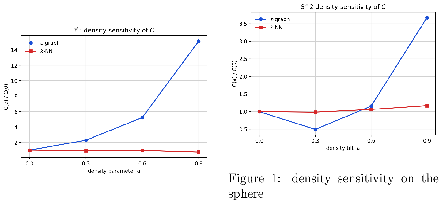
References↩︎

---

1. Corresponding author↩︎