1 Introduction↩︎

A learned world model is typically trained to reconstruct what it observes or to predict the reward it receives, and its quality is then reported as a single number: a reconstruction error, or a return under planning. This treats fidelity as something a model either has or lacks. But a model that reconstructs its inputs perfectly can still be useless for control, and a model that predicts reward well can fail to support the longer-horizon reasoning a task demands. What a world model should capture is not its observations in general but the structure its downstream queries actually depend on—the small set of collective coordinates that carry those queries and evolve together under the dynamics. We call this set the queries’ closure, and we take model quality to be how much of the closure a trained latent comes to represent. Ask where the Moon will be at midnight: the closure is six slowly drifting orbital elements, no matter how many pixels of night sky we record.

The objective a model is trained against is the lever that installs, or fails to install, that structure. The dominant choice in model-based reinforcement learning is value equivalence: rather than model the world faithfully, learn a model that predicts value or reward correctly, on the grounds that nothing else matters for acting well. Value equivalence is attractive precisely because it is low-dimensional—a scalar value signal is cheap to predict and is aligned with the quantity the agent ultimately cares about. This raises a question that, to our knowledge, has not been put directly to a trained deep world model: does an aligned scalar objective install the structure a controllable task needs, or only a shadow of it?

We answer this on a DreamerV3 stack in a controlled environment, where a known low-dimensional process is rendered into high-dimensional observations so that the ground-truth closure is available for comparison. The answer is that a scalar objective installs only a one-dimensional projection. Training the latent against an aligned scalar value and then reading the closure out of it with a linear probe recovers a small fraction (\(0.10\)) of what the same probe recovers from a latent trained against the full, multi-dimensional objective (\(0.76\)). The gap is not an artifact of the probe or the architecture—the network, the probe, and the training budget are identical—but of the objective’s dimensionality. Sweeping that dimensionality from one to four installs exactly one, two, three, and four predictive directions in turn, and a one-dimensional objective whose weight is raised to match the four-dimensional objective’s total training pressure still installs a single direction. The same staircase appears when the objective is the model’s own value head rather than an auxiliary regression, at attenuated magnitude, so the difference in head form does not account for it. The structure a latent represents tracks the dimensionality of what it is asked to predict.

This sharpens, rather than refutes, the value-equivalence principle. Proper value equivalence is defined over a set of value functions and may be high-dimensional; what is insufficient is the ubiquitous single-reward instantiation, the rank-one corner of a law in which a \(d\)-dimensional objective installs \(d\) closure directions. Read constructively, the result gives a quantitative answer to how much value equivalence a task needs: at least the rank of its closure. The law also has a boundary, and we measure it rather than assume it. On a companion closed-loop control stack whose closure is directly observable frame by frame, a single scalar reward matches a full value family in installed rank and in executed return. Reconstruction without any reward installs the same closure: where the observations hand a task’s structure to reconstruction, the objective is moot (Section 9). Objective dimensionality governs the complement—the regime in which reconstruction does not recover the closure—and the environment below is built to sit there. We make no claim about natural images; the environment is a measurement instrument, built so that a failure to represent the closure is a matter of allocation rather than availability (Section 2). Our contributions are:

• a direct demonstration, on a learned deep world model, that the rank a latent installs equals the dimensionality of the objective it is trained against—swept from one to four and reproduced through both an auxiliary head and the model’s own value head;

• the value-equivalence rank-one corner as a within-system dissociation: an aligned scalar and a full objective, matched in stack, probe, and budget, install \(0.10\) and \(0.76\) of the same closure;

• a measured boundary for the law: where the closure is frame-observable, single-reward value equivalence matches a full value family in rank and return, and reconstruction alone installs the closure; and

• a reduced-rank account of the ceiling, sharpened from an optimal-readout bound to a gradient-flow prediction, with a pre-committed falsifier.

We also connect the training-side law to evaluation: the discounted Bellman residual decomposes by construction into a reward term and the \(\gamma\)-scaled value-only operator error, so a Bellman-residual score reads only the value slice of a model’s dynamics. We give supporting evidence on released models (Section 8) and defer the full treatment to a companion paper [1].

2 Closure and the controlled environment↩︎

A family of queries closes under the dynamics when a low-dimensional set of coordinates carries every query in the family and evolves approximately autonomously, so that the queries’ future can be predicted from those coordinates alone. The closure is the minimal such set, and the question of what a model represents is the question of which closure directions are recoverable from its latent state.

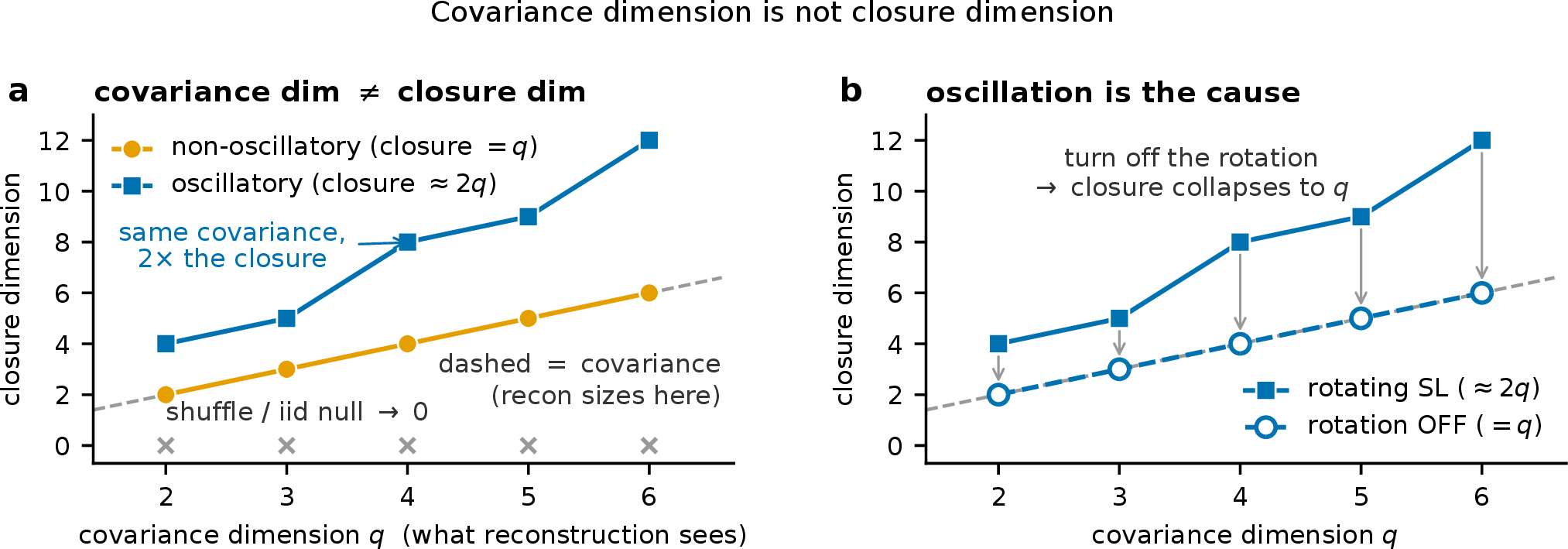
Reconstruction targets the wrong object. The dimension a signal occupies in covariance is not the dimension its prediction requires: a single oscillating mode fills one direction of the observation covariance but spans a two-dimensional predictive subspace, because forecasting it requires both its phase components (its sine and cosine components—equivalently, position and velocity). A reconstruction or covariance objective therefore systematically under-sizes the closure (Figure 2), which is the basic reason fidelity to the observation does not imply fidelity to the query.

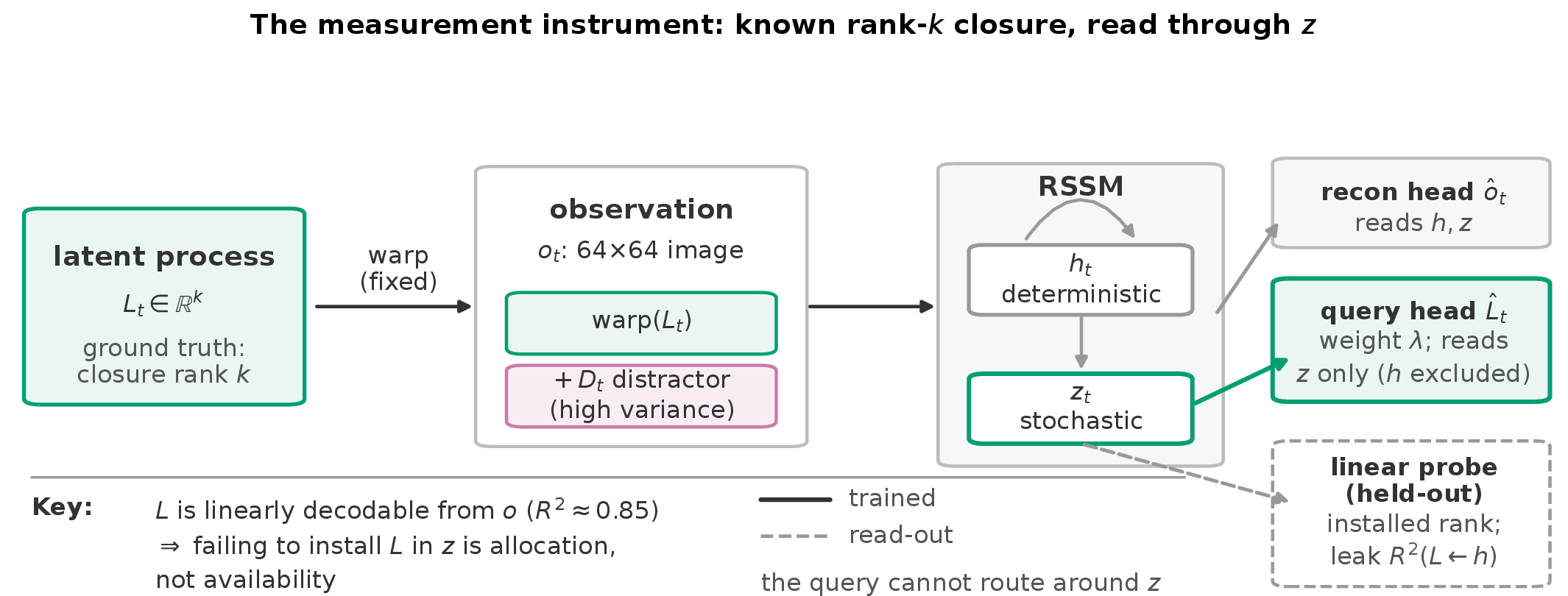
We study this in a controlled environment built on a DreamerV3 categorical-RSSM stack [2]. A known process of \(k\) slowly varying latent coordinates is rendered through a fixed analytic warp into a \(64\times64\) image observation. Because the construction is ours, the closure rank is known and the latent coordinates are linearly decodable from the observation, at \(R^2 \approx 0.85\). We make no natural-image claim: the environment is a measurement device rather than a perception benchmark, and the linear decodability is what lets us attribute any failure to represent the closure to how the model allocates its latent, not to whether the information is there to be represented.

3 Method↩︎

We train the world model with its usual reconstruction objective augmented by an auxiliary head that predicts the query target with weight \(\lambda\), and we read what the latent has learned with a linear probe. Two choices make the readout interpretable. First, the auxiliary head and the probe both act on the stochastic latent alone; the deterministic recurrent state is excluded, so a query cannot be satisfied through a pathway the latent itself does not carry. Second, we summarize what is represented by the installed rank: the number of closure coordinates a linear probe recovers from the latent above a threshold set by a reconstruction-only null (the per-column null mean plus \(2.5\) standard deviations, fixed post hoc; the readouts are unchanged across the \(+2\) to \(+3\sigma\) band). Alongside the installed rank we report the total recoverable structure (\(R^2\) of the full closure from the latent) and a leakage check verifying that the closure is not instead readable from the excluded recurrent state. Figure 3 summarizes the instrument.

4 The objective, not reconstruction, determines the representation↩︎

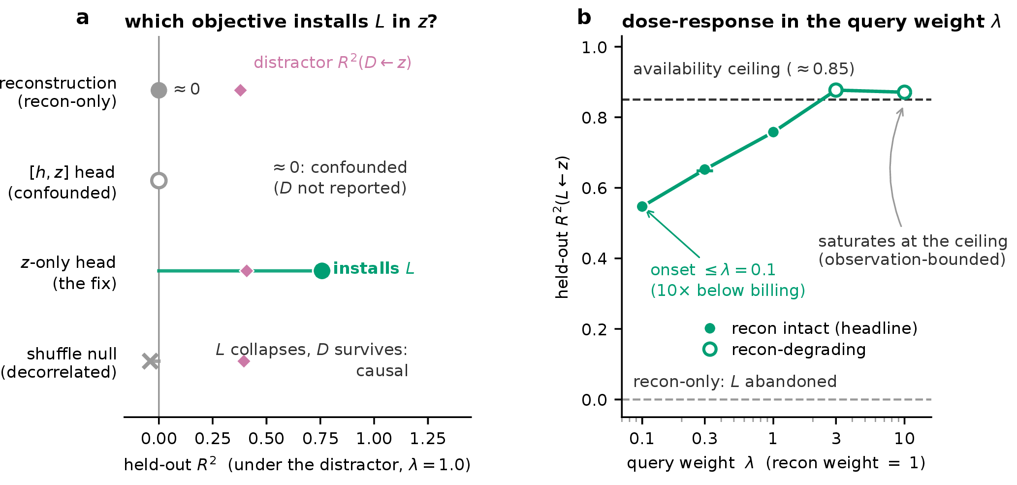
Before asking which objectives install the closure, we establish that an objective installs it at all. We place a high-variance distractor in the observation alongside the low-variance query coordinates, so that a model minimizing reconstruction error is drawn to the distractor and away from the query. An auxiliary head allowed to read both the latent and the recurrent state leaves the query unrecoverable from the latent—but this is an artifact of architecture, not of the objective, because the head routes the query through the recurrent state and drains the latent. Once the head is forced onto the latent alone, the picture reverses (Figure 4). A query-aligned objective installs the closure in the latent even under the distractor, with recovery climbing as the objective weight increases (from \(0.55\) to \(0.88\)) and saturating at the level to which the closure is linearly present in the observation, while reconstruction remains intact. The dependence is causal: shuffling the query labels during training collapses recovery to zero while the distractor stays readable, so it is the objective, not an incidental correlate, that determines what the latent holds. A recovery gate fixed in advance confirmed that the latent could represent the closure before we measured how strongly the objective installs it. This determination is exercised only where the environment forces it: where reconstruction already recovers the closure, the objective has nothing left to decide—the boundary we quantify in Section 9.

5 Value equivalence is the rank-one corner↩︎

5.1 An aligned scalar objective installs a single dimension↩︎

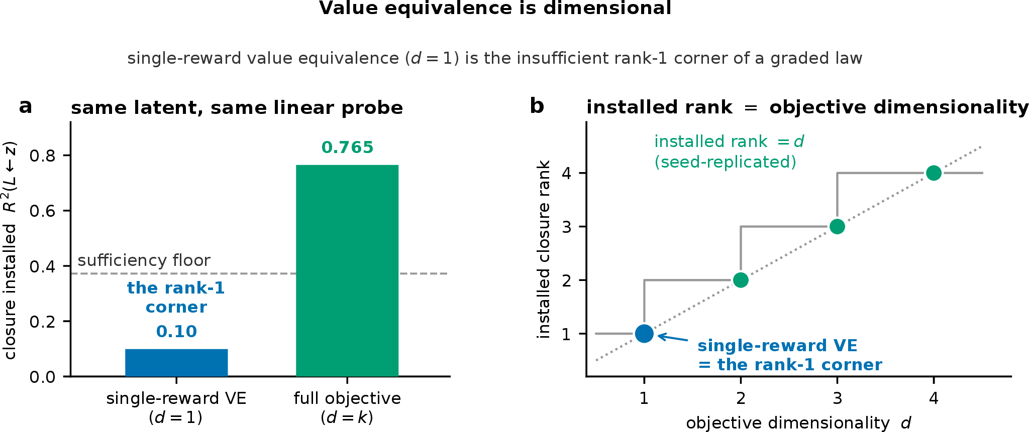
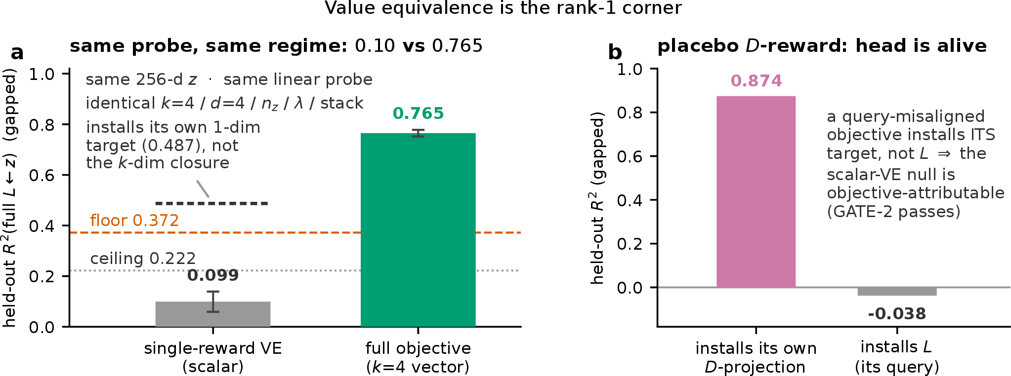
We now replace the multi-dimensional query target with an aligned scalar: a single value/reward signal of exactly the kind value equivalence prescribes, predicted through the model’s value head. Although the scalar is perfectly aligned with the task, the latent it installs contains almost none of the query closure. A linear probe recovers \(R^2 = 0.10\) of the full closure, far below the \(0.37\) install floor and well below the \(0.76\) the same probe recovers from a latent trained on the full objective in the same configuration (\(k=4\), \(n_z=4\), \(\lambda=1\) in both arms; Figure 5).¹ The scalar does install its own one-dimensional projection (\(0.49\)), so the head is working as intended, and a placebo objective built from the distractor installs the distractor (\(0.87\)) but not the query—so the head is capable of installing structure when the structure it is asked for is present. The shortfall is specific to the scalar’s dimensionality, not a failure of the probe or the head. In plain terms: the model asked to predict value learned the value—and almost nothing else the task depends on.

5.2 Installed rank tracks objective dimensionality↩︎

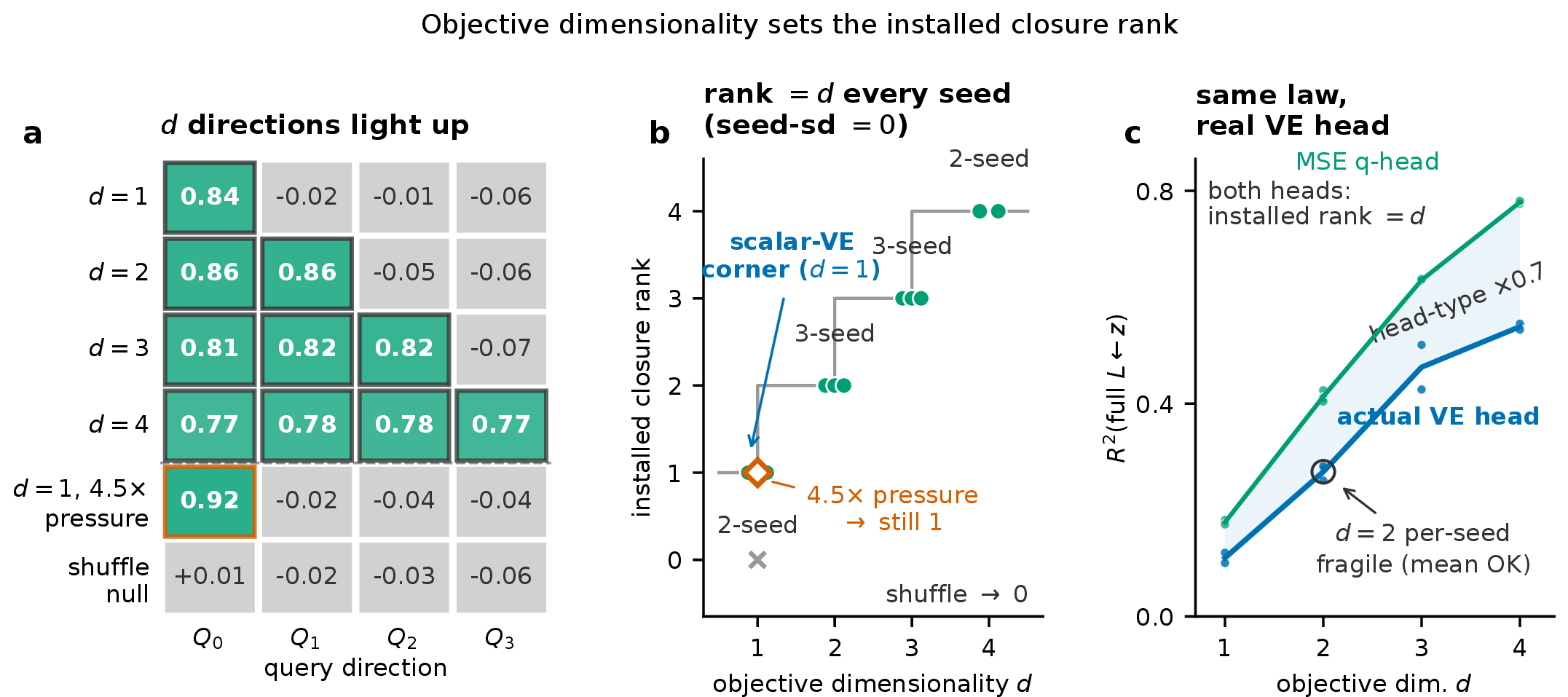
The scalar’s failure is the lower end of a graded law. Holding the architecture and the head fixed, we vary only the dimensionality \(d\) of the objective’s target from one to four. The number of closure directions installed in the latent follows exactly: one, two, three, and four (Figure 6). The effect is dimensionality, not training pressure: raising a one-dimensional objective’s weight 4.5-fold—to the four-dimensional objective’s total target variance—still installs a single direction. The ramp does strengthen that one direction (its recovery rises to \(0.92\)) but recruits no second: the unsupervised directions stay at the reconstruction null, so what tracks dimensionality is the number of installed directions, not their magnitude. The latent holds as many directions as the objective asks for—no more, and asking harder for one does not buy a second. The staircase reproduces across seeds at every step—three seeds at the interior \(d=2,3\), two at the endpoints, and every seed lands on installed rank \(d\). Reduced-rank regression supplies the reason (Section 6): the rank of the structure an objective can install is bounded by the rank of its target, so a \(d\)-dimensional objective installs at most \(d\) directions, and empirically it installs exactly \(d\). Single-reward value equivalence sits at \(d=1\); the closure of a controllable task generally does not.

5.3 The same law through the value head↩︎

The sweep above varies dimensionality through an auxiliary regression head, whose form differs from the value head that value equivalence actually uses. To remove that difference we repeat the sweep through the model’s own value head, supervising a \(d\)-dimensional family of value/reward functions—the set over which proper value equivalence is defined—and reading the installed rank as before. The law survives the change of head. Averaged over seeds (three at \(d=2\), two at each other \(d\)), a \(d\)-dimensional value objective installs \(d\) closure directions for \(d\) from one to four, and the rotation-invariant total recovery climbs monotonically with \(d\) (\(0.11\), \(0.27\), \(0.47\), \(0.55\)), each dimension’s readout band separated from the next. Because every cell of this sweep is installed by the same value head, head type no longer co-varies with dimensionality—the confound the single matched comparison of Section 5.4 could not fully remove.

The recovered magnitudes are about \(0.7\times\) the regression head’s at matched \(d\). The value head also warps its target through \(\tanh\), but on these slowly varying, near-unit-variance coordinates the warp is near-linear (a linear fit recovers \(R^2\approx0.93\) of the target variance), so this attenuation is attributable to head type, not to a distinct nonlinear target encoding—and it leaves the rank intact. The per-seed \(d=2\) count is threshold-fragile, so the law is stated on the three-seed mean and the total-recovery overlay rather than a per-seed count. The remaining caveats—the magnitude attenuation, the borderline \(d=2\) coordinate, and the sweep’s uncontrolled aggregate pressure—are detailed in Appendix 13.

5.4 A matched-dimension control↩︎

The scalar and the full objective compared above differ not only in dimensionality but in the form of their prediction head and target encoding. To isolate dimensionality from these, we compare, at identical task dimension and capacity, a full multi-dimensional target against the scalar: the former installs the closure (\(0.76\), a wide margin above the leakage ceiling²) and the latter does not (\(0.10\)). This is consistent with the dimensionality reading and removes the cross-task confound. Head type and target encoding still co-vary within this single comparison, but the head-type difference is separated directly by the value-head sweep of Section 5.3, which installs rank \(d\) through the same value head at each interior dimension; the matched pair is retained as same-regime support, no longer the load-bearing evidence for that separation.

6 Why dimensionality bounds the representation↩︎

The ceiling is reduced-rank regression in another guise. If the objective’s target spans \(d\) dimensions, the cross-covariance between target and latent has rank at most \(d\), so the population-optimal linear predictor occupies at most \(d\) directions of the latent, and which \(d\) directions—the leading canonical directions of the target–latent cross-covariance—is fixed by the same canonical-correlation truncation that underlies our closure spectrum [3]–[5]. The bound is independent of how much capacity the latent carries: a wider latent does not install more of the objective’s structure, only the same \(d\) directions. This is the objective-side counterpart of value equivalence [6]—the objective’s rank, not the model’s size, caps the closure a latent installs.

The bound constrains the optimal readout; what training installs is a separate question, and in the linear case gradient descent answers it. For a linear encoder and linear head trained by gradient flow on the query loss, the coupled dynamics learn the modes of the target–latent cross-covariance one at a time, in order of their canonical correlation, converging to the rank-\(d\) reduced-rank regressor—the top-\(d\) canonical directions and no more [7], [8]. So attainment is not, in this case, a separate empirical fact but the gradient-flow prediction: training installs exactly \(d\) directions whenever the target covariance has rank \(d\) and all \(d\) canonical correlations are strictly positive—a zero canonical correlation is a target direction the objective cannot reach, and would lower the count. This turns the earlier “\(\le d\) bound, \(=d\) empirical” into “\(=d\) is the gradient-flow prediction,” which the experiments then verify one architecture up.

We borrow this rigor rather than claim it, and two fences keep the borrowing honest. First, the theory is linear—both the \(\le d\) readout bound and the \(=d\) gradient-flow attainment are proved for a linear encoder and head, whereas every model here uses a nonlinear head; the transfer is to the rank a linear probe can read, and the gradient-flow prediction is one we verify in the nonlinear stack rather than inherit, under a no-spillover regularity—unsupervised target coordinates stay at the reconstruction null and a label shuffle collapses the readout—that stands in for the linear theory’s guarantees. Second, the capacity-independence is demonstrated synthetically; on the trained pixel stack the analogous install fails to generalize across distributions for reasons orthogonal to this bound (Section 9).

The same algebra suggests a falsifiable companion. Under a shared capacity budget the model must allocate latent directions between reconstruction and the query, and the reverse-water-filling intuition of rate–distortion theory [9] predicts a greedy, marginal-value ordering: tight capacity makes the query displace reconstruction, abundant capacity makes it add to it. We state this as a prediction with a pre-committed falsifier—the installed rank must plateau at \(d\) with shielded coordinates at the null, and is refuted by a continued rise or a genuinely installed extra direction—and we do not derive the threshold itself (Appendix 14). The same lens links the two sides of the paper: when the objective is value alone, the Bellman residual decomposes by construction into a reward term and the \(\gamma\)-scaled value-only operator error, so value equivalence is the low-dimensional slice on the evaluation side as well (Section 8). The contribution throughout is the law’s behavior in a trained deep model and its falsifiable form, not a new theorem. A stronger, ordinal reading of the same heuristic—installation in proportion to marginal value, not merely up to a count—survives only in part when tested one level below this ceiling: on a trained pixel stack of four graded-predictability targets the converged install magnitude runs counter to the predictability order across three seeds (seed-mean rank correlation \(-0.56\); the second-most-predictable direction installs weakest in every seed), while install timing partially recovers it. This bounds the magnitude refinement of the allocation heuristic only; the rank ceiling, its attainment, and the confirmed rank-ramp falsifier are untouched (Appendix 14.4).

7 Calibration and a prospective test↩︎

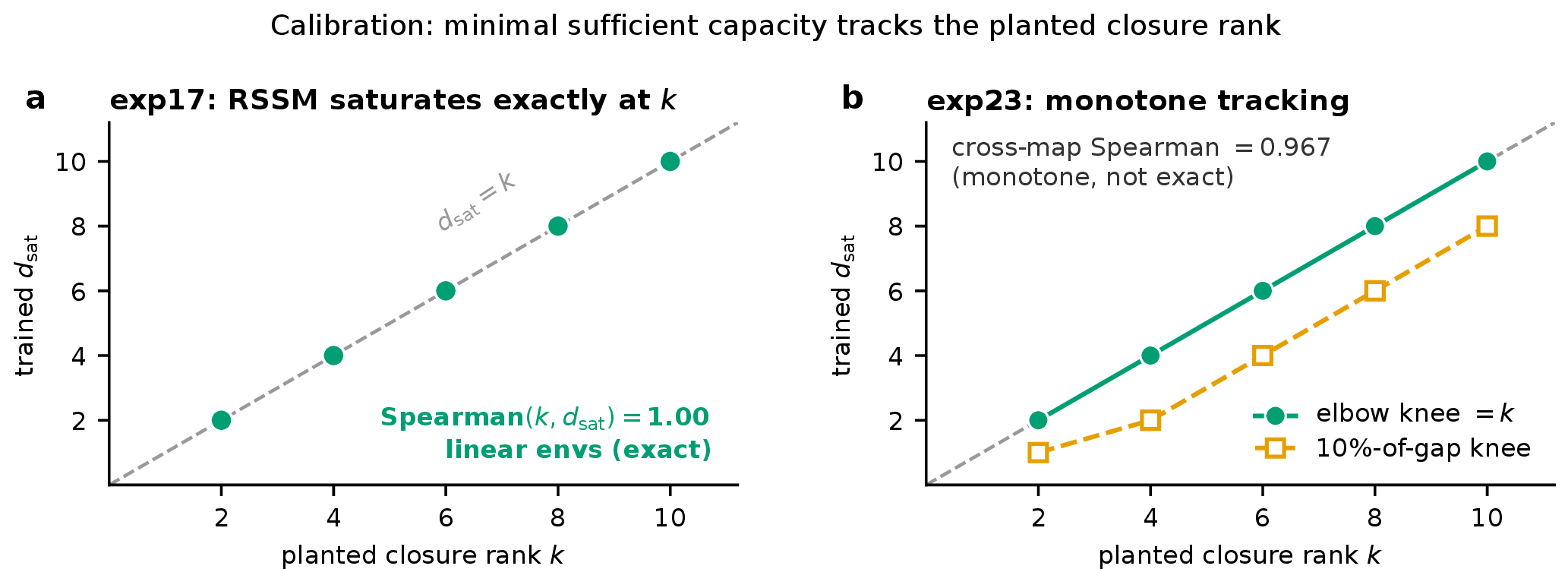
Two checks anchor the readout against ground truth. First, in a continuous-latent version of the environment, the installed rank rises with capacity and then plateaus at the objective dimension \(d\), holding through a latent several times larger than the closure; the plateau level tracks \(d\), not capacity, with the exact knee tolerance-relative. A categorical latent of the kind the main stack uses instead saturates at a fixed level regardless of size, as predicted by the rate–rank distinction: \(n_z\) categorical variables over \(C\) classes carry about \(n_z\log_2 C\) bits and can spread partial information over more than \(n_z\) closure directions, so capacity binds as a rate, whereas a continuous latent of width \(n_z\) binds as a rank of \(n_z\) (Appendix 14.3; Figure 7). This was registered as a prediction of the dimensionality law before it was run, and it is distinct from the trained stack’s continuous-latent variant, whose generalization failure is reported in Section 9. Second, on planted environments whose closure rank is known by construction, a trained model’s minimal sufficient latent tracks that rank—exactly on the simplest family and monotonically once the observation map is varied (Figure 8). Both are synthetic calibrations and are labeled as such; the capacity term in particular is established only synthetically.

8 The evaluation side↩︎

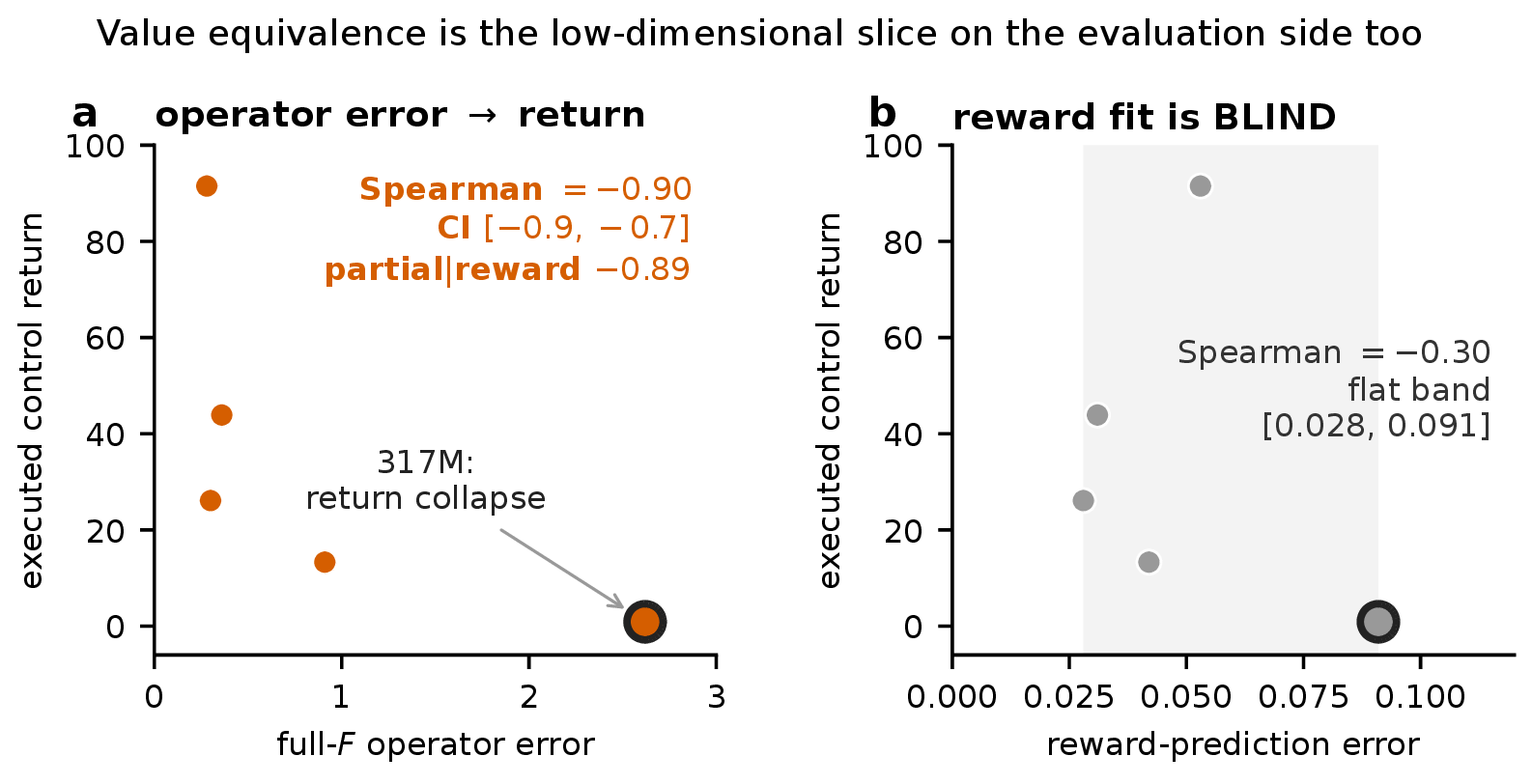
The same low-dimensional character appears on the evaluation side, where a model is judged by how it rolls forward. The discounted Bellman residual decomposes by construction into a reward term and the \(\gamma\)-scaled value-only operator error (Appendix 14.7), so scoring a model by its Bellman residual reads only the value slice of its dynamics—and a full operator that also tracks non-value structure can pull apart from it. On released TD-MPC2 checkpoints [10] the reward error is two orders of magnitude below the value term, and full-operator error tracks executed return (\(\mathrm{Spearman}=-0.90\); \(n=5\) sizes on one task, correlational) while reward-prediction error does not (Figure 9). This is the evaluation-side echo of the training-side rank-one install; we present it as supporting evidence and defer the full cross-architecture treatment—a different axis, operator fidelity rather than representational content—to a companion paper [1].

9 Scope and limitations↩︎

9.0.0.1 Where the objective matters.

The law’s regime is not universal, and we measured its boundary directly rather than assuming it. On a closed-loop control stack whose four-coordinate closure is directly observable frame by frame (a single-frame decode reaches \(R^2\approx0.998\) per coordinate), single-reward value equivalence is indistinguishable from a full value family in installed rank—posterior and open-loop rollout alike—and in executed return, and an action-masked reconstruction arm installs the same closure with no reward signal at all (Figure 10a; Appendix 13). Where the observations hand the closure to reconstruction, the objective is moot. The corollary is a bounded sufficiency result for practice: when a task’s return-relevant closure is frame-observable, single-reward value equivalence suffices in closed loop. The rank-one corner is a risk for passive prediction and for tasks whose closure is not observable, not a universal control deficiency. Where the screen already shows the state, any objective—or none—will do.

9.0.0.2 The cheapest-channel ordering.

The boundary appears to generalize by training channel. A coordinate that is only transiently observable is also installed without objective pressure: the recurrent state carries it to its point of use, and this free carry decays to chance within about forty-five steps while a supervised, objective-installed coordinate stays durably at ceiling over the same lags—a threshold-free contrast that replicates on all three seeds (Figure 10b; Appendix 13). This suggests an ordering with a common currency. Intuitively: if the model can see a coordinate, reconstruction learns it; if it just saw it, recurrence carries it; if it can infer it from how observations respond to actions, filtering completes it; only what none of these reach must be paid for by the objective. Formally, fix the data-collecting policy \(\pi\), and say a coordinate is reached by a channel when it is measurable with respect to that channel’s information set. These sets are nested—the current-frame \(\sigma\)-algebra (what reconstruction sees) \(\subseteq\) the history \(\sigma\)-algebra (what recurrence carries) \(\subseteq\) the history closed under one-step dynamics inversion (what a recurrent filter can complete)—so a coordinate installs through the cheapest channel that reaches it: reconstruction, then recurrence, then filtering, with the objective the channel of last resort. Objective dimensionality then gates representation exactly for coordinates that are return-relevant but measurable with respect to none of the three passive sets (return-relevant, unobservable, and unfilterable) (Figure 11). We state the channel-level observations (reconstruction and recurrence install for free where they reach) as replicated, and the ordering itself as a synthesis those observations support but do not yet establish.

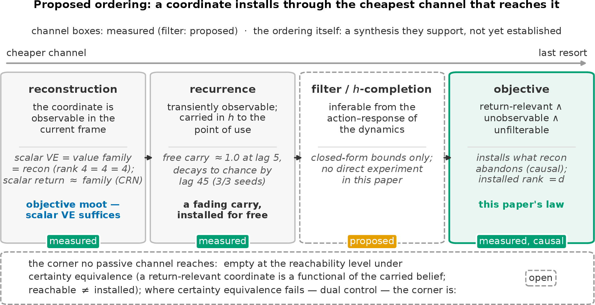
The sharpest question the ordering poses is whether any coordinate exists that only the objective can install. Under the fixed policy \(\pi\), a coordinate is passively reachable exactly when it is measurable with respect to \(\Sigma_{\mathrm{obs}}(\pi)\), the observation \(\sigma\)-algebra generated under \(\pi\) (the union of the three nested passive sets above). The corner is therefore empty precisely when every return-relevant direction lies in that set—the completeness statement \(\Sigma_{\mathrm{val}}\subseteq\Sigma_{\mathrm{obs}}(\pi)\)—and this is a stronger condition than certainty equivalence: a return-relevant coordinate that \(\pi\)’s observations never excite is unreachable by any passive channel regardless of whether the value function factors through the belief. Where completeness fails—dual control, where acting to gather information has value the passive prediction problem never sees—the corner can be non-empty; that edge is open, and we claim nothing about it here.

9.0.0.3 Limitations.

Our evidence comes from a single architecture, a single environment family, and a synthetic observation, chosen so that ground truth is available; we do not claim the law holds unchanged on natural images, and the capacity term is established only synthetically. The continuous-latent variant carries an honest negative: the closure it installs is genuine on the training distribution but does not transfer to fresh rollouts, even though the closure remains linearly present in those rollouts—a generalization failure we have not been able to attribute to a mechanism. On a public world-model benchmark [11], our linear closure estimator reaches only about a third of the relevant structure and the test is underpowered at the sixteen available environments, so we report it as a boundary on the instrument rather than a test the thesis passes or fails.

10 Related work↩︎

Value equivalence and its proper, set-valued refinement frame our question [6], [12]; we sharpen rather than overturn them. Value-aware model learning derives model objectives from the value functions they must serve [13]–[15], and MuZero is the scaled instance of training a model only on reward, value, and policy [16]; our result measures how much of a task’s structure that family of objectives installs, as a function of its dimensionality.

On the representation side, auxiliary prediction tasks have long been used to shape what an agent’s features carry [17], the geometry of a set of value functions is known to determine the representation they induce [18], [19], and task-informed world models discard observation structure a target deems irrelevant [20]–[22]; what we add is the closure as the reference object and the rank law for how much of it an objective of a given dimensionality installs.

The bound we use is reduced-rank regression [3]–[5], and the closure object is the stochastic-realization and canonical-correlation reading of minimal predictive state [23]–[25], with predictive-state representations supplying the rank side [26], [27]. Our contribution is empirical—a demonstrated mechanism in a learned deep world model, and a falsifiable form of it—rather than a new theorem.

11 Conclusion↩︎

In the regime where reconstruction does not recover a task’s closure, what a world model represents is set by the dimensionality of the objective it is trained against—not by its capacity, its observations, or the magnitude of a scalar reward; where reconstruction does recover it, the objective is moot, a boundary we measured rather than assumed. Value equivalence is dimensional, and its familiar single-reward form is the rank-one corner of that law. How much value equivalence a task needs is, to first order, the rank of its closure—and whether it needs any depends on whether that closure is already in view. The Moon we began with was, by this light, the easy case: all six of its coordinates are offered to any patient observer, no objective required. The rank-one corner is reserved for the structure the sky keeps to itself.

12 Method and readout conventions↩︎

We train a DreamerV3 categorical-RSSM world model [2] with its standard reconstruction objective augmented by an auxiliary query head of weight \(\lambda\), and we read what the latent has learned with a linear probe applied after training. Both the auxiliary head and the probe act on the stochastic latent \(z\) alone: the deterministic recurrent state \(h\) is excluded from the head’s forward pass and from the probe, so a query cannot be satisfied through a pathway the latent itself does not carry. This is the single most consequential design choice—a head free to read \([h,z]\) routes the query through \(h\) and leaves \(z\) holding the distractor, an architecture artifact documented in Appendix 13.

We summarize what a latent represents by its installed rank: the number of closure coordinates a linear probe recovers from \(z\) above a per-column threshold. The probe is a ridge regression with held-out regularization; for each closure coordinate \(L_i\) we report the held-out, gap-corrected \(R^2(L_i\!\leftarrow z)\) (recovery in excess of a same-capacity baseline), and count a coordinate as installed when this exceeds \(\tau_{\mathrm{col}}\), the reconstruction-only per-column null mean plus \(2.5\) standard deviations. The anchor is fixed by inspecting the null pool rather than pre-registered, and the installed-rank readouts are unchanged across the \(+2\) to \(+3\sigma\) band (Appendix 13). Alongside the installed rank we always report the total recoverable structure \(R^2(\text{full }L\!\leftarrow z)\), the full convention panel across thresholds, and a leakage check \(R^2(L\!\leftarrow h)\) confirming the closure is not instead readable from the excluded recurrent state.

A linear probe reports only the linearly-readable rank, a lower bound on what the head may have installed nonlinearly; where the distinction matters we cross-check with a one-hidden-layer probe. Before measuring the dose-response of Section 4 we verified, with a pre-registered recovery gate, that the latent can represent the closure at all in the absence of the distractor (recovery \(0.87\)–\(0.89\)); only then did we measure how strongly the objective installs it under the distractor.

13 Additional controls and negative results↩︎

We treat the negative and confounded results as part of the evidence; this appendix collects the controls behind the main claims.

13.0.0.1 The architecture confound and its fix.

Our first auxiliary head read both \(z\) and the recurrent state \(h\). Under the distractor this left the closure unrecoverable from \(z\), but as a control it is confounded: the head routes the query through \(h\) and drains \(z\) even without the distractor. We therefore force the head onto \(z\) alone (Appendix 12), which makes the leak structurally impossible (\(R^2(L\!\leftarrow h)\le 0.04\)). The honest reading is that the permissive head is a well-verified but architecture-confounded null and the \(z\)-only head is the clean test.

13.0.0.2 Causal control.

To confirm that the objective, not an incidental correlate, installs the closure, we shuffle the query labels across the training set with everything else fixed. Recovery collapses to \(-0.040\) (the reconstruction null) while the distractor stays readable (\(R^2(D\!\leftarrow z)=0.395\)): the install is driven by the supervised target.

13.0.0.3 Dimensionality vs.pressure.

The pressure-matched control of Section 5.2 raises a one-dimensional objective’s weight to the four-dimensional objective’s total target variance (\(4.5\times\)). This matches the objective weight, not the achieved gradient magnitude: the realised gradient norm of the one-dimensional control (\(0.069\)) did not reach the four-dimensional objective’s (\(0.316\)). The pressure confound is therefore ruled out not by this control alone but directly, in situ: under the ramp the already-installed direction does strengthen in magnitude—its recovery rises from \(0.84\) to \(0.92\) (Figure 6a)—but no second direction lights up, the unsupervised coordinates staying at the reconstruction null. It is the number of installed directions, not their magnitude, that tracks dimensionality; extra pressure on one direction does not recruit another. Pressure, in short, cannot pull rank. (The magnitude of the installed directions is roughly flat across the \(d\)-sweep as well, but that is a weaker observation and we do not lean on it.)

13.0.0.4 Threshold robustness.

The per-column threshold \(\tau_{\mathrm{col}}\) is anchored post hoc to the reconstruction-only null; the installed-rank staircase is unchanged across the \(+2\) to \(+3\sigma\) band, so the readout does not depend on the particular anchor within that range. The threshold is not load-bearing for a more basic reason (Figure 12): every supervised column is recovered at \(R^2\approx0.8\) and every unsupervised column at \(\approx-0.05\), so \(\tau_{\mathrm{col}}\) and its whole band fall inside a \(\sim\) \(0.8\)-wide empty gap between the two—any anchor in that gap yields the same staircase.

13.0.0.5 Leakage in the matched pair.

In the single matched-dimension comparison of Section 5.4 the closure is marginally readable from the excluded recurrent state (\(R^2(L\!\leftarrow h)\approx 0.04\), just over our \(0.03\) purity bar)—a ridge-decode artifact where the target dimension approaches the probe’s effective degrees of freedom; the sweep cells of Section 5.2 satisfy the bar.

13.0.0.6 The value-head sweep.

Repeating the dimensionality sweep through the model’s own value head over a \(d\)-dimensional value/reward family (\(d=1\)–\(4\)) separates objective dimensionality from head form. The seed-mean staircase (three seeds at \(d=2\), two at each other \(d\)) installs rank \(1,2,3,4\) with total recovery \(0.11,0.27,0.47,0.55\), about \(0.7\times\) the regression head’s magnitudes at matched \(d\). The per-seed count at \(d=2\) is threshold-fragile: one seed’s leading unsupervised coordinate (\(0.026\)) grazes the null threshold (\(\approx 0.025\)) and changes sign across seeds (\(+0.026,-0.018,-0.043\); mean \(-0.012\)), so the law is stated on the three-seed mean and the total-recovery overlay, not a per-seed count. The aggregate training pressure is not held constant across the sweep—the value-head loss rises roughly ninefold from \(d=1\) to \(d=4\)—so dimensionality is separated from pressure by the in-situ proxies and the pressure-matched control of Section 5.2, as in the regression sweep, rather than by a matched design here.

13.0.0.7 The knee recalibration.

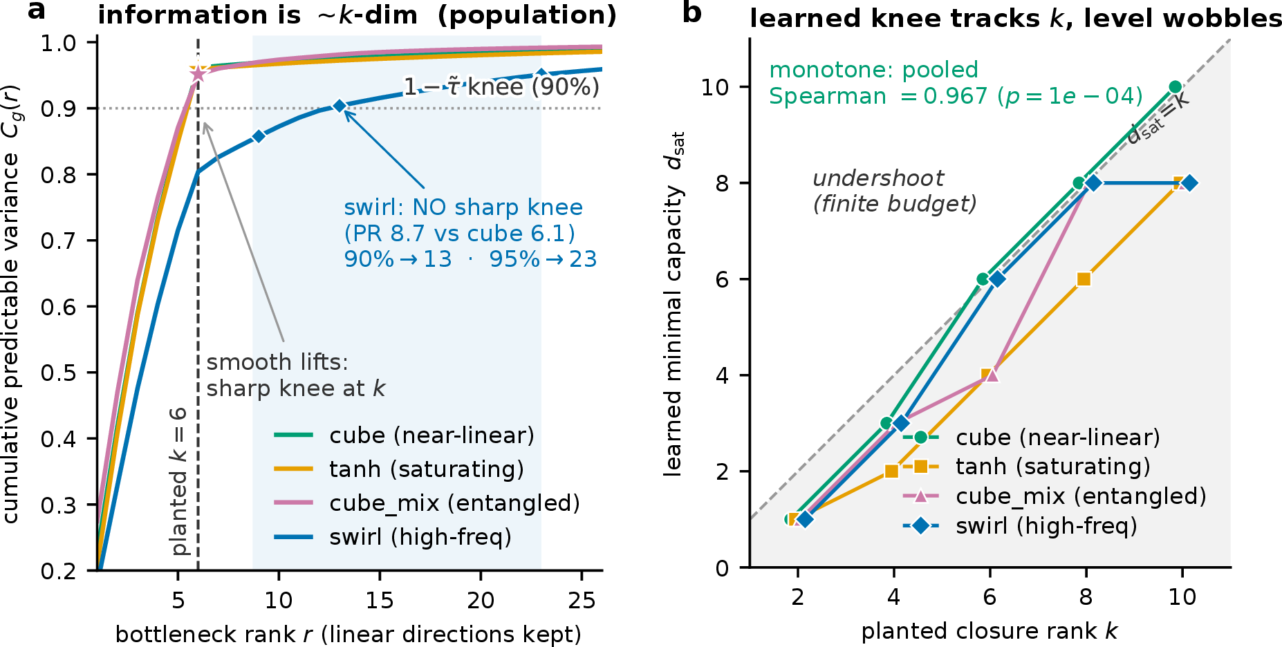
In the planted-rank calibration (Appendix 16) the exact “saturates at \(k\)” claim is convention-relative: under a stricter knee rule the trained capacity under-reads. We retain the diffeomorphism-invariant statement (minimal capacity tracks the closure rank monotonically) and treat the convention-dependence of the exact knee as a disclosed property of the estimator, not a hidden failure (Figure 13).

13.0.0.8 Reconstruction sufficiency (the scope boundary).

The three arms behind Figure 10a—single-reward value equivalence, a full value family, and action-masked reconstruction with no reward—are trained on the frame-observable control task quantified in Section 9 (single-frame decode \(R^2\approx0.998\) per coordinate). All install the same rank-\(4\) closure in posterior and open-loop rollout alike, and the value-equivalence arm’s return matches the family’s under common random numbers on every seed, so none of the main-text dissociations appear where reconstruction already recovers the closure.

13.0.0.9 The recurrence carry and its decay.

In a partially observed variant in which a cue is visible only transiently, arms trained with reconstruction alone still carry the cue to its point of use: the recurrent state holds it with no objective pressure. Read at increasing lags, this free carry decays from near-perfect to chance by lag \(45\) on all three seeds, while an arm that receives the cue through a supervised objective stays at ceiling across the same lags on all three seeds (Figure 10b). The contrast is a decay curve, not a single-lag binary—a pre-registered single-lag threshold read of the same data proved seed-fragile and was retired as a scorer, which we report rather than quote—and it separates supervised from passive channels, not a distinct “value channel” from supervision. It is the evidence behind the ordering suggested in Section 9.

14 Reduced-rank ceiling and the allocation law↩︎

This appendix collects the borrowed rigor behind the bound of Section 6. None of it is a new theorem: the linear-algebraic backbone is classical, cited in each statement, and we use it only to account for the shape of an empirical law in a trained deep model. We first recall the closure-spectrum identities the bound rests on, then state the ceiling and its proof sketch, then the rate–distortion allocation law (separating what is derivable from what is borrowed intuition), and finally the two scope fences, the pre-committed falsifier, and the evaluation-side reduction.

14.1 Closure spectrum: the linear backbone↩︎

Take a linear–Gaussian system \(x_{t+1}=Ax_t+w_t\) with a linear query \(y=Cx\), and stack the horizon-\(H\) future query \(f_t=[y_{t+1};\dots;y_{t+H}]=O_H x_t + N_t\), where \(O_H\) is the observability map and \(N_t\perp x_t\) the irreducible future noise. With reachability Gramian \(W_c=\mathrm{Cov}(x_t)\) and \(M:=W_c^{1/2}O_H^\top\), three facts organize everything downstream.

14.1.0.1 Lemma 1 (spectrum identity).

The population canonical correlations \(\rho_i\in[0,1]\) between past and future query are the singular values of \(M\,\Sigma_{ff}^{-1/2}\), and the deterministic Hankel singular values \(\sigma_i\) are the singular values of \(M\) itself. The two share rank and range exactly—\(\#\{\rho_i>0\}=\#\{\sigma_i>0\}=\dim(\text{closure})\), with the same closure subspace—and share ordering under isotropic predictable-coordinate noise; the magnitudes coincide only up to the noise normalization. That past/future canonical correlations are the stochastic-realization Hankel singular values is classical canonical variate analysis [4]; we use only its rank/range content.

14.1.0.2 Theorem 1 (rank-\(d\) error \(=\) floor \(+\) tail).

In the whitened query metric, the best rank-\(d\) predictor’s relative error decomposes exactly as \[\mathrm{err}(d)^2 \;=\; \underbrace{1-\tfrac{1}{qH}\textstyle\sum_i \rho_i^2}_{\mathrm{floor}^2} \;+\; \tfrac{1}{qH}\textstyle\sum_{i>d}\rho_i^2 ,\] each added dimension removing exactly \(\rho_{d+1}^2/qH\) of error. The tail bookkeeping is reduced-rank regression / canonical-correlation truncation [3], [5], [28]; the named, co-equal floor term and the exact orthogonal split are what the present program treats as a first-class axis.

14.1.0.3 Corollary 1 (minimal sufficiency).

The number of canonical correlations above a tolerance \(\tau\) is the minimal model dimension past which each further direction buys less than \(\tau^2/qH\) of query variance—a property of the dynamics, query, horizon, exploration, and feature class, not of any model. This is the Hankel-rank result shared by balanced truncation [25] and spectral learning of predictive states [29]; we add only its relativity to the full tuple.

14.2 The reduced-rank ceiling↩︎

Write \(L\in\mathbb{R}^k\) for the closure the query depends on and \(z\in\mathbb{R}^{n_z}\) for a learned latent. Suppose an objective supervises the first \(d\le k\) coordinates \(L_d=U^\top L\) (\(U\in\mathbb{R}^{k\times d}\)) of the closure through \(z\), and write \(\mathrm{installed}_L\) for the rank a linear probe can read out of \(z\).

14.2.0.1 Statement (linear head).

For a linear head forming the population-optimal prediction of \(L_d\) from \(z\), the relevant cross-covariance \(\Sigma_{L_d,z}=U^\top\Sigma_{L,z}\) has rank at most \(\mathrm{rank}(U^\top)=d\), so the optimal predictor occupies at most \(d\) directions of \(z\). With the empirical premise that reconstruction installs essentially none of \(L\) in the regime where the distractor is the reconstruction-salient direction (verified: the reconstruction-only readout of \(L\) collapses to the null), this gives \[\boxed{\;\mathrm{installed}_L \;\le\; d, \quad\text{independently of } n_z.\;}\] The rank-\(d\) ceiling is Eckart–Young [3]; the load-bearing content—which \(d\) directions install, namely the leading canonical directions of the \((L,z)\) cross-covariance—is the canonical-correlation truncation of Lemma 1 / Theorem 1 [4], [5]. The “\(\le\)” is the theorem; equality (that the installed rank attains \(d\) rather than falling short) is empirical. The result is the objective-side counterpart of value equivalence [6]: the objective’s rank caps the installed closure.

14.2.0.2 Proof sketch.

Supervising only \(L_d=U^\top L\) makes the target–latent cross-covariance factor through \(U^\top\), of rank \(\le d\); the best rank-constrained linear map from \(z\) to that target is its reduced-rank / canonical-correlation truncation, whose row space has dimension \(\le d\) [3], [4]. Capacity \(n_z\) enters only as the ambient dimension of \(z\) and cannot raise the cross-covariance rank, so the bound is capacity-independent. The reconstruction term, by the empirical premise, contributes no additional \(L\)-direction.

14.2.0.3 From an optimal-readout bound to a gradient-flow prediction.

The statement above bounds an optimal linear readout; the empirical claim is about what training installs. In the linear case the two coincide, and this upgrades “\(=d\) is empirical” to a training-dynamics prediction. For a linear encoder and linear head trained by gradient flow from small initialization, learning proceeds mode by mode in order of the canonical correlations of the target–input cross-covariance, converging to exactly its top-\(d\) canonical directions—the deep-linear learning dynamics of [7], [8], whose fixed point is the reduced-rank / canonical-correlation truncation already invoked. So for a linear stack \(\mathrm{installed}_L=d\) is not only the ceiling but the gradient-flow limit, and our nonlinear-stack measurement (installed rank \(=d\) at every \(d\)) is the verification that the prediction carries over. Equality (rather than \(\mathrm{installed}_L<d\)) requires two conditions, which sharpen the falsifier: the supervised target’s covariance must have full rank \(d\), and all \(d\) of its canonical correlations with the recoverable latent must be strictly positive; a rank-deficient target or a vanishing canonical correlation installs strictly fewer than \(d\) directions.

14.3 The allocation law: derivable ordering vs.borrowed intuition↩︎

The latent has finite capacity, so a model trained on reconstruction-plus-query solves a constrained allocation. We separate two registers.

14.3.0.1 Derivable.

At a constrained optimum the marginal unit of capacity goes to whichever direction yields the largest marginal loss reduction—a greedy marginal-value ordering. This much is the standard convex-allocation argument and is all that is genuinely derivable here.

14.3.0.2 Borrowed intuition (not derived).

The reverse-water-filling solution of rate–distortion theory [9] supplies the picture for that ordering, but it is a single-source, single-distortion, single-budget result and does not instantiate the present two-objective problem (reconstruction distortion versus query distortion sharing one budget); reducing the two to one water-filling problem requires a common marginal-value currency on a jointly-Gaussian basis, which is a modeling assumption, not the theorem. The regime statements are therefore predictions the heuristic makes, labeled as such: under tight capacity the query displaces reconstruction (a one-sided shedding, with the two readouts not summing to a conserved budget); under abundant capacity the query adds, with \(\mathrm{installed}_L=d\) and reconstruction retained. On a continuous latent, capacity binds as a rank (\(n_z\) independent directions); on a categorical latent it binds as a rate (about \(n_z\log_2 C\) bits), so a single categorical direction can carry partial information about more than \(n_z\) closure directions at once and the rank form takes the wrong functional shape—which is why the capacity claims are made on a continuous (or synthetic-continuous) latent and why a categorical latent saturates by finer quantization rather than by adding directions. The threshold at which displacement turns into addition is itself tolerance-relative and ordinal, never a sharp integer; we do not derive it.

14.4 The marginal-value ordering, tested one level below the ceiling↩︎

The rank ceiling fixes how many directions install and the canonical-correlation truncation names which ones; the allocation heuristic adds a stronger, ordinal claim—that under a flat objective the directions install in proportion to their marginal value, i.e.their dynamical predictability. We tested this refinement on a trained pixel stack supervising four modal targets of distinct predictability (\(\rho=0.98,0.90,0.80,0.65\)), reading both each direction’s installed magnitude and its install timing. Unlike the scoped-out generalization negative of Appendix 14.5, the install here is present on fresh episodes—that is the premise of the test—so what is at issue is not whether the directions install but how strongly.

The magnitude half of the prediction does not hold. Across three seeds the converged install magnitude runs counter to the predictability order (per-seed rank correlations \(-0.67,-0.67,-0.33\); mean \(-0.56\)), the stable anomaly being that the second-most-predictable direction (\(\rho=0.90\)) installs weakest in every seed. Install timing, by contrast, partially recovers the predictability order (first-crossing rank correlation \(+0.33\), all three seeds), so it is the converged magnitude, not the arrival order, that departs. The obvious confounds are ruled out in this stack: a same-architecture, dynamics-free convolutional control recovers all four directions at \(R^2\approx0.999\) (so the effect is not encoder readability), the per-direction target variances are isotropic to within \(3.5\%\) (not a scale artifact), and the loss has plateaued (not under-training). We do not identify the mechanism here; a separate line probes it interventionally.

This recalibrates the borrowed intuition, not the theorem, and along an axis the paper has already found fragile. Just as the planted-rank saturation knee is estimator-relative while its monotone ordering survives (Appendix 13), here a magnitude—the relative install strength—is stack-relative; the parallel is that a magnitude recalibrates in both, not that the ordering is equally kept—the install timing order here is only sign-stable (\(\tau=+0.33\) across three seeds), far short of the knee’s near-perfect ordinal survival. The rank bound (\(\mathrm{installed}_L\le d\)) and its attainment (\(=d\)) are untouched: all four directions clear the reconstruction-only per-column null. This magnitude result is moreover distinct from—and does not dent—the confirmed ordinal shape of the rank falsifier (Appendix 14.6, the sub-\(d\) ramp rising into a plateau at \(d\)): that shape concerns how the count fills as capacity grows, not the relative strength of the \(d\) directions at fixed capacity. The invariant the paper rests on is the rank; the relative magnitude with which its directions install is not.

14.5 Two scope fences↩︎

14.5.0.1 Linear head vs.nonlinear head.

The ceiling is proved for a linear head; every experiment here uses a nonlinear head, whose input–output Jacobian is not rank-\(\le d\). The bound therefore transfers only to the linearly-readable rank—what a linear probe extracts—and only under an empirical no-spillover regularity: under ramped query pressure the unsupervised coordinates of \(L\) stay at the reconstruction null, a label shuffle collapses the readout, and reconstruction alone installs none of \(L\). We never present the nonlinear-head experiments as instances the linear theorem proves.

14.5.0.2 Synthetic vs.pixel.

The capacity-independent half—installed rank rising then plateauing at \(d\) as the latent grows past the closure—is demonstrated on a synthetic continuous latent. The trained pixel stack is a separate, scoped-out generalization negative: there the install is real on the training distribution but fails to generalize to fresh rollouts even though the signal is present in the fresh observations, an encoder-generalization failure with no positively identified mechanism. It is orthogonal to the rank-axis bound and is not explained or rescued by this appendix.

14.6 The pre-committed falsifier↩︎

So that a flexible law cannot absorb any outcome, we pre-commit, before the run and on a continuous low-rate latent: the rank form is confirmed iff the installed rank plateaus at \(d\) through a latent at least twice the closure rank, with the unsupervised coordinates at the reconstruction null and non-overlapping supervised/unsupervised readout bands; it is refuted by a continued rise with capacity or by a genuinely installed extra direction in shielded coordinates. The invariant is the ordinal shape—a sub-\(d\) ramp rising into a plateau at \(d\)—rather than an exact integer count, since the count inside the ramp is tolerance-relative. The synthetic calibration shows this criterion is testable rather than vacuous: it resolves a plateau at \(d=3\) from a plateau at \(d=4\) by the objective dimension, not by capacity.

14.7 The evaluation-side reduction↩︎

The same low-dimensional reading appears on the evaluation side. At an anchor \((s_t,a_t,s_{t+1})\) let \(\hat{z}'\) be the model’s one-step latent rollout and \(z'=\mathrm{enc}(s_{t+1})\) the encoded true next state, with reward error \(\Delta r=r_{\text{model}}-r_{\text{true}}\) and value-only operator error \(\Delta v=V(\hat{z}')-V(z')\). The discounted Bellman residual decomposes by construction: \[\big|(r_{\text{model}}+\gamma V(\hat{z}'))-(r_{\text{true}}+\gamma V(z'))\big| \;=\; |\Delta r + \gamma\,\Delta v|, \qquad \big|\,\text{Bellman residual} - \gamma\,|\Delta v|\,\big| \;\le\; |\Delta r| .\] When the reward head is exact (\(\Delta r=0\)) the Bellman residual equals \(\gamma\) times the value-only operator error exactly; when the reward error is small relative to the value term, the two are near-identical and agree in rank. This is elementary—the affine one-step backup telescoped into its reward and value parts—and we present it as a standard observation, not a theorem. The identity is written for a single sampled transition; for stochastic dynamics the Bellman residual carries an expectation over next states (\(r+\gamma\,\mathbb{E}_{s'}V(z')\)) and the same telescoping holds in expectation, while our per-anchor operator error is the sampled form, applied anchor-by-anchor. On released models the reward error is two orders of magnitude below the value term, so the (unnormalized) value-only operator error and the Bellman residual are empirically near-identical; the normalized \(\{r,V\}\) slice, a different aggregate, is not. Value equivalence is thus the low-dimensional slice on the evaluation side as it is on the training side.

15 Evaluation-side protocol↩︎

The evaluation-side result of Section 8 is reported in full in a companion paper [1]; we summarize the protocol here. For a model with encoder \(\mathrm{enc}\) and \(k\)-step latent rollout \(O_k\), and an observable subset \(F\), the operator error at an anchor \((s_t,a_{t:t+k-1},s_{t+k})\) compares the model’s rolled-forward latent \(\hat{z}_{t+k}=O_k(z_t,a_{t:t+k-1})\) to the encoded true next state \(z'_{t+k}=\mathrm{enc}(s_{t+k})\), by reading each functional \(\phi\in F\) off both through a shared ridge probe and aggregating the normalized per-anchor errors. The value slice sets \(F=\{r,V\}\) using the model’s own reward and value heads; the full aggregate adds a per-anchor PCA basis on the encoded next-state geometry, fit on a held-out half of the anchors so it cannot adapt to operator error.

We evaluate released TD-MPC2 checkpoints [10] on the DeepMind Control cheetah-run task [30] at five parameter counts (\(1\)M–\(317\)M), at a matched five-step horizon. Across the sweep, reward-prediction error stays in \([0.028,0.091]\) while the full-operator error spans \(0.28\) to \(2.62\); the full-operator error tracks executed return at Spearman \(-0.90\) (anchor-bootstrap CI \([-0.90,-0.70]\), leave-one-out \(\le -0.80\); \(n=5\) sizes, correlational), whereas the Bellman residual and reward error track return only weakly (\(-0.10\) and \(-0.30\)). The unnormalized value-only operator error is rank-identical to the Bellman residual across the sweep (Spearman \(+1.00\)), consistent with the decomposition of Appendix 14.7; the normalized value slice is not (\(+0.10\)). The full cross-architecture comparison and additional controls are deferred to the companion paper [1].

16 Environment construction and synthetic protocols↩︎

16.0.0.1 The controlled testbed.

The main experiments use a controlled latent-recovery environment: a known low-dimensional process of \(k\) slowly varying latent coordinates is rendered through a fixed analytic (cubic) warp into a \(64\times64\) image observation, with a high-variance distractor added alongside the low-variance query coordinates. The query coordinates modulate \(k\) Gaussian blobs at fixed, well-separated positions and the distractor modulates full-frame low-frequency fields, spatially entangled so that every pixel carries both contributions and a convolutional encoder cannot ignore the distractor by receptive-field masking. The closure rank is therefore known by construction, and the query coordinates are linearly decodable from the observation at \(R^2\approx 0.85\), so any failure to represent them reflects how capacity is allocated rather than a missing signal. The world model is the DreamerV3 categorical-RSSM stack [2], trained to convergence. The dose–response of Section 4 uses \(k=2\) closure coordinates; the corner comparison and both dimensionality sweeps of Section 5 use \(k=4\) with latent capacity \(n_z=4\).

16.0.0.2 Capacity (continuous-latent) calibration.

To separate capacity from objective dimensionality we replace the categorical latent with a continuous one and sweep its width past the closure rank. The installed rank rises with capacity and plateaus at the objective dimension \(d\) (the plateau level tracks \(d\); the exact knee is tolerance-relative), holding through a latent several times the closure rank; a categorical latent of the kind the main stack uses instead saturates at a fixed level regardless of width, consistent with its capacity binding as a rate rather than a rank (Appendix 14.3). This run was pre-registered as a test of the rank-form prediction, with the falsifier of Appendix 14.6 fixed before it was executed.

16.0.0.3 Planted-rank calibration.

As a ground-truth check on reading rank off a trained model, we plant environments whose closure rank \(k\) is known and ask where a trained model’s minimal sufficient latent \(d_{\mathrm{sat}}\) saturates. On the simplest (linear) family \(d_{\mathrm{sat}}=k\) exactly (Spearman \(1.000\)); as the observation map is varied across analytic lifts (cube, tanh, and mixtures) the minimal capacity tracks \(k\) monotonically (pooled Spearman \(0.967\)), with the exact knee level convention-relative (Appendix 13). All synthetic and planted results are labeled as calibration and are never read as natural-image rank results.

16.0.0.4 Covariance vs.closure.

The teaching panel of Section 2 uses a single oscillatory mode, which occupies one direction of the observation covariance but spans a two-dimensional predictive subspace; shuffling or replacing the dynamics with noise collapses the closure on both axes.

17 Capacity reallocation↩︎

At tight capacity the allocation law of Appendix 14.3 predicts that installing the query displaces the distractor rather than adding to it. At a latent width equal to the closure rank, as the query weight \(\lambda\) rises the recovered distractor falls monotonically (Spearman \(\rho_D(\lambda)=-1.0\)) while the recovered query rises (\(\rho_L(\lambda)=+0.94\)); the two do not sum to a conserved budget, consistent with one-sided shedding rather than a fixed-budget rank trade. The displacement is reproduced across seeds at the clean interior weight, where the install is partial and the latent carries both (\(R^2(L\!\leftarrow z)\approx 0.42\) while \(R^2(D\!\leftarrow z)\approx 0.29\)); the full monotone shape at larger \(\lambda\) is single-seed and entangled with degrading reconstruction. We therefore report displacement as a confirmed tight-capacity prediction and the precise high-\(\lambda\) trajectory as suggestive.

18 Benchmark probe↩︎

As a check on whether the closure estimator says anything on a real combinatorial benchmark, we apply it to the publicly runnable subset of AutumnBench [11]. From a fixed uniform-random exploration protocol we estimate, per (environment, query-family) cell, the closure’s effective rank and linear error floor, and ask whether these separate the environments the released models scale on from those they saturate on. They do not: across the sixteen publicly runnable environments the per-family separations are consistent with chance (stratified within-family permutation \(p=0.53/0.75/0.98\) on the floor, effective-rank, and action-corrected excess axes; AUC \(\approx 0.5\)), while shuffle and i.i.d.controls collapse as expected (Figure 14).

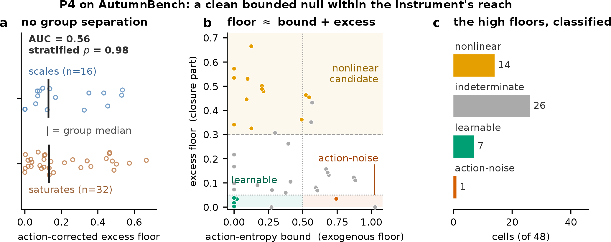
Two bounds make this a statement about the instrument rather than a test the thesis passes or fails. First, it is underpowered: only sixteen of the forty-three scored environments are publicly runnable, so a moderate effect could not be distinguished from noise. Second, the linear estimator reaches only about a third of the relevant closures (roughly seventeen of forty-eight cells have a recoverable linear floor); the rest would need a nonlinear estimator to be tested at all. We therefore report AutumnBench as the boundary at which our linear instrument stops being informative on a discrete combinatorial benchmark, and as motivation for a deeper estimator—not as evidence for or against the dimensionality law.

References↩︎