When Do Geometric Algebra Layers Beat Scalarization?
A Controlled Study on SO(3)-Equivariant Vector Laws
July 07, 2026
Abstract
Compact networks built from Clifford algebra \(\mathrm{Cl}(3,0)\) primitives (grade-wise equivariant linear maps, geometric products, grade gates) are exactly SO(3)-equivariant and learn synthetic 3D vector laws from few samples. We ask whether the geometric algebra structure itself contributes anything beyond exact equivariance. We compare against a minimal scalarization baseline: invariant dot products fed to a small MLP that outputs coefficients on the equivariant basis \(\{v_i,\, v_i \times v_j\}\), which is also exactly equivariant. On single-stage laws (rotation by axis-angle, cross product, central force), scalarization matches or beats the \(\mathrm{Cl}(3,0)\) network at a fraction of the training cost, so the geometric algebra adds nothing there. On compositional targets whose computation graph nests group operations (apply \(R_2 R_1\) to a point; map a local force through an orientation, then take a torque), the \(\mathrm{Cl}(3,0)\) network beats scalarization by an order of magnitude in the low-data regime, reaching with 100 samples the accuracy the baseline achieves with 3000, and the gap survives strengthening the baseline with the triple-product invariant and 17x more parameters, external Vector Neurons and e3nn baselines, and a multiplicative coefficient network. Ablations show the required network depth tracks the rotation chain length, and scalarization falls below the constant predictor on chains of four rotations. The advantage is not composition per se: on a rotation-free nested cross product, which flattens into polynomial invariant coefficients, scalarization wins by 24x. On the torque task the advantage is confined to low data, with a crossover near a thousand samples. No tested model, equivariant or not, extrapolates invariant magnitudes: on radius and separation shifts every model is worse than a constant predictor once errors are normalized. We conclude that geometric algebra layers are not a general shortcut for low-data 3D learning, but become useful precisely when the target composes group elements in depth.
1 Introduction↩︎
Many 3D learning problems require functions that commute with rotations: a predicted force, torque, or displacement should rotate with the input frame. Equivariant architectures encode this constraint in the parameterization, and small-scale demonstrations routinely show large sample-efficiency gains over unconstrained networks. Such demonstrations, however, usually conflate two distinct effects: (a) restricting the hypothesis class to equivariant functions, and (b) the specific parameterization of the proposed architecture. Effect (a) is available from a trivial construction. By classical invariant theory, every SO(3)-equivariant vector-valued function of vectors \(v_1,\dots,v_k\) can be written as \(\sum_j c_j(\text{invariants})\, b_j\), where the \(b_j\) range over the inputs and their pairwise cross products and the \(c_j\) are functions of the SO(3) invariants of the inputs: the pairwise dot products and, for orientation-sensitive (chiral) targets, the scalar triple products \(v_a \cdot (v_b \times v_c)\) [1]. Learning the \(c_j\) with a small MLP gives an exactly equivariant model that we call scalarization. Our base scalarization uses the dot-product invariants; the strengthened variant adds the triple products, and the two tasks with three or more inputs (two-body, nested cross) test whether that matters.
This paper asks a narrow question: does a small geometric algebra network built from \(\mathrm{Cl}(3,0)\) bilinear layers offer anything that scalarization does not? We answer it with a controlled benchmark of six synthetic vector laws, normalized metrics, tuning controls, and strengthened baseline variants. Our contributions are negative and positive results of equal importance:
On single-stage laws, those computable with one equivariant interaction (rotation of a point, cross product, central force), scalarization matches or beats the geometric algebra network, at 13 to 19x lower training cost (Section 5, Finding 2).
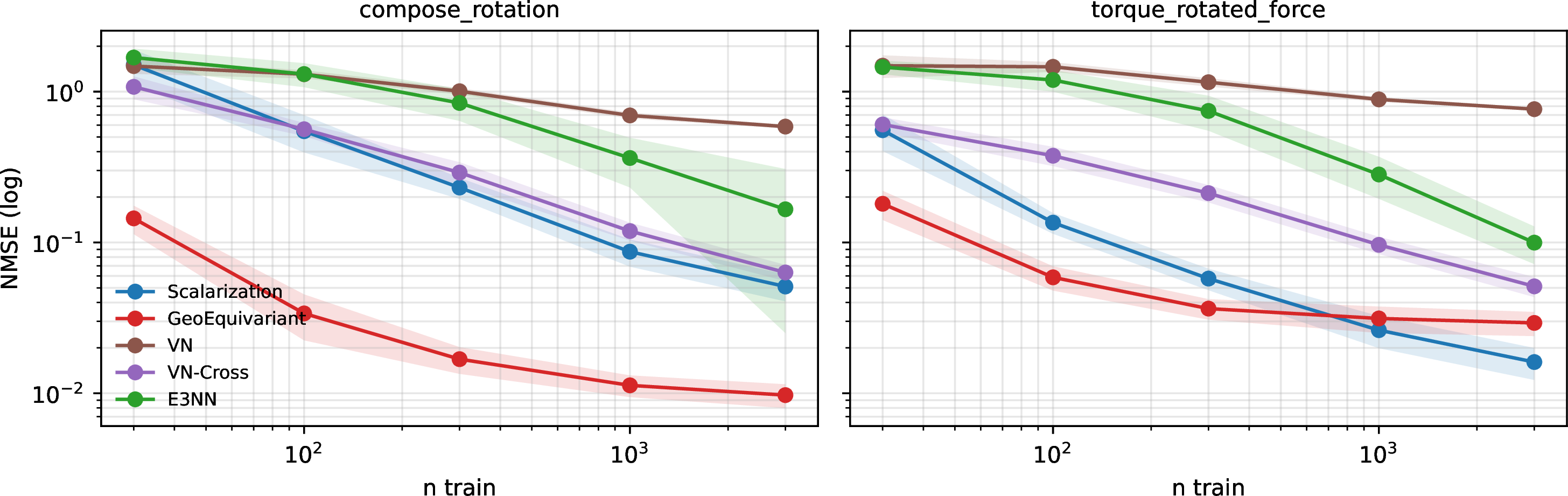
On compositional laws, those whose computation graph nests group operations (composition of two rotations, local-to-world torque), the geometric algebra network wins by 3x to 16x in the low-data regime and under angle shift, and the gap survives capacity and feature strengthening of the baseline; on the torque task scalarization catches up beyond a thousand samples (Finding 3, Figure 1).
No tested model extrapolates invariant magnitudes. On radial out-of-distribution splits, every model, equivariant or not, is worse than a constant predictor once errors are normalized (Finding 4). Unnormalized MSE hides this failure, which we argue is a reporting pitfall for equivariance benchmarks.
2 Related work↩︎
Equivariant deep learning encodes group symmetry in the architecture [2], [3]. For 3D rotations, irreducible-representation approaches include Tensor Field Networks [4], the e3nn framework [5], and steerable networks [6]; lighter-weight constructions include Vector Neurons [7] and E(n)-equivariant graph networks [8]. Equivariance is known to improve data efficiency in the sciences [9]. Geometric (Clifford) algebra architectures embed inputs as multivectors and use the geometric product as the core operation [10]–[12]. On the analysis side, [1] characterize equivariant functions through scalar invariants, which directly motivates our scalarization baseline, and [13] study the universality of rotation-equivariant models. Closest to our baseline, [14] express equivariant targets as scalar functions multiplying a small tensor basis; closest to our geometric model, GLGENN [15] builds parameter-light Clifford equivariant networks. Unlike GATr, which scales a projective geometric algebra transformer to large scenes, we work at the opposite end: a minimal controlled benchmark isolating what the algebra contributes. Our contribution is not a new architecture: it is a controlled delimitation of when the geometric product parameterization pays relative to the scalarization construction that theory already provides.
3 Models↩︎
All models map 6 or 9 input dimensions (two or three 3D vectors) to one 3D vector and are trained identically: Adam, full batch, 200 epochs, learning rate \(5\times 10^{-3}\), mean squared error. A grid over learning rate and epochs (Section 6) confirms that no conclusion is an artifact of this choice.
3.0.0.1 MLP (7.4k parameters).
Three hidden ReLU layers of width 58 on the flattened input. Unconstrained reference.
3.0.0.2 MLP-Aug.
The same MLP trained with 8x random SO(3) data augmentation, rotating all input vectors and the target with the same rotation.
3.0.0.3 Scalarization (1.3k to 1.5k parameters).
All pairwise dot products of the \(k\) input vectors feed a two-layer MLP of width 32 that outputs one coefficient per basis element \(\{v_i\} \cup \{v_i \times v_j\}_{i<j}\); the output is the coefficient-weighted sum. Exactly SO(3)-equivariant. For \(k=3\) a strengthened variant adds the scalar triple product \(v_1 \cdot (v_2 \times v_3)\) to the invariants, making orientation-sensitive information directly available to the coefficient network.
3.0.0.4 Vector Neurons (2.4k to 2.6k parameters).
An external equivariant baseline [7]: channels are 3D vectors, linear layers mix channels with learned scalars, and the VN-ReLU nonlinearity projects each feature on the halfspace defined by a learned direction. Faithful to the original design, the output lies in the linear span of the input channels, so a two-vector input cannot produce a cross product. We therefore also test VN-Cross, the common practical fix that appends pairwise cross products of the inputs as extra channels.
3.0.0.5 E3NN (6.6k to 11k parameters).
A second external baseline built from irreducible-representation tensor products, the standard construction behind irreps equivariant models [4], [5]. Inputs are \(l{=}1\) irreps, each block is a self tensor product gated by scalar channels with an equivariant BatchNorm, and the norm of each input vector is expanded into a small Gaussian radial basis fed as extra scalar channels. This radial embedding is standard in irreps models [9] and was necessary here: without it the network cannot represent functions of an angle magnitude and stays worse than a plain MLP on the rotation task. As this benchmark is SO(3) rather than full O(3), all irreps use a single parity, which sidesteps a channel-pruning failure mode we observed when mixing parities.
3.0.0.6 GeoBilinear (28k parameters).
Inputs are embedded as multivectors of \(\mathrm{Cl}(3,0)\) (8 components per channel: vectors on grade 1, axis-angle inputs on grade 2 via duality). Three stacked blocks compute \(\mathrm{gp}(Ax, Bx) + Cx\) where \(\mathrm{gp}\) is the geometric product and \(A, B, C\) are unconstrained linear maps on multivector channels, followed by a grade-norm gate and channel normalization. Ablation control: geometric products without the equivariant constraint.
3.0.0.7 GeoEquivariant (2k parameters).
The same architecture with grade-wise weight tying (one scalar per grade per channel pair), which makes every layer exactly SO(3)-equivariant. Measured relative equivariance error is \(2\times 10^{-7}\), the float32 limit. The augmented MLP, for comparison, reaches 0.22 to 0.49 depending on the task.
4 Tasks and protocol↩︎
Inputs are standard normal unless stated. Train and test sets use disjoint random generator seeds; out-of-distribution (OOD) splits use disjoint input regions, verified numerically. Five seeds per configuration; we report mean normalized MSE (NMSE): test MSE divided by the MSE of the constant mean predictor on the test targets. NMSE 1.0 equals a trivial predictor. We use NMSE because raw MSE is misleading under distribution shift: on far-radius splits the targets are small, so a failing model still gets a small raw MSE.
rotation: \((u, p) \mapsto R(u)\,p\) with \(u\) an axis-angle vector. OOD: unseen axis hemisphere; unseen angle range \([\pi/2, \pi]\) after training on \([0, \pi/2]\).
cross: \((a, b) \mapsto a \times b\). OOD: unseen hemisphere.
central force: \((r, d) \mapsto -r/(\lVert r\rVert^3 + 0.05)\) with a distractor input \(d\). OOD: radii \([1.25, 3]\) after training on \([0.25, 1]\).
two-body force: \((r_1, r_2) \mapsto -(r_1 - r_2)/(\lVert r_1 - r_2\rVert^3 + 0.05)\). OOD: separations \([2, 4]\) after training on \([0.5, 1.5]\).
composed rotations: \((u_1, u_2, p) \mapsto R(u_2) R(u_1)\, p\). OOD: unseen hemisphere for both axes.
local-to-world torque: \((r, u, f) \mapsto r \times (R(u) f)\), a local force mapped to the world frame and applied at a lever arm, the minimal robotics composition. OOD: unseen axis hemisphere; unseen angle range.
We call tasks 1 to 4 single-stage: their targets require one equivariant interaction of the inputs, possibly modulated by a learned function of invariants. Tasks 5 and 6 are compositional: their computation graph nests group operations. All tasks lie within the intended approximation class of both equivariant model families, and neither family faces a symmetry-induced expressivity obstruction on these targets, so differences measure optimization behavior and inductive fit rather than hard expressivity gaps.
5 Results↩︎
5.1 Finding 1: exact equivariance dominates, whatever its construction↩︎
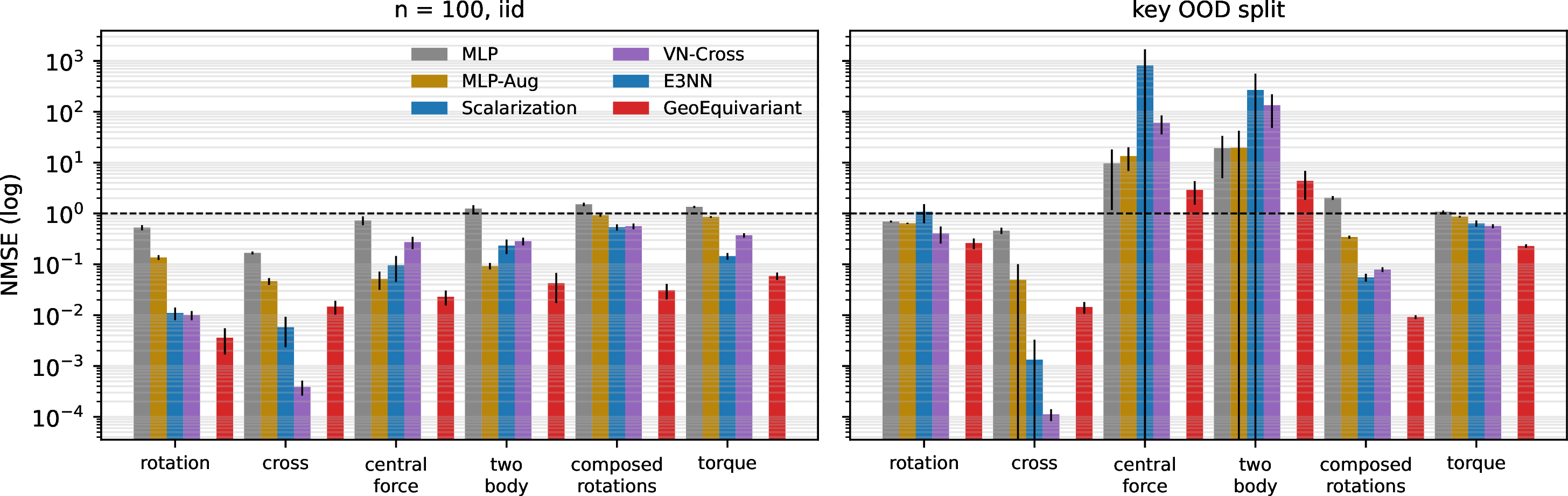
At \(n{=}100\) on the rotation task, NMSE is 0.53 for the MLP, 0.14 for the augmented MLP, 0.011 for scalarization and 0.0036 for GeoEquivariant. Augmentation reduces the measured equivariance error (0.28 to 0.22) but stays 10 to 20x behind the exact constructions on directional OOD splits. This pattern holds on all six tasks (Table 1, Table 2).
5.2 Finding 2: on single-stage laws, scalarization is enough↩︎
| Task | Model | Params | \(n{=}100\) iid | \(n{=}1000\) iid | OOD | s/run |
|---|---|---|---|---|---|---|
| rotation | MLP | 7427 | \(0.53 \pm 0.06\) | \(0.101 \pm 0.006\) | \(0.61 \pm 0.07\) | 1.0 |
| rotation | MLP-Aug | 7427 | \(0.14 \pm 0.01\) | \(0.054 \pm 0.005\) | \(0.064 \pm 0.007\) | 3.9 |
| rotation | Scalarization | 1283 | \(0.011 \pm 0.003\) | \(0.0040 \pm 0.0016\) | \(0.0033 \pm 0.0011\) | 0.6 |
| rotation | VN | 2424 | \(0.46 \pm 0.02\) | \(0.41 \pm 0.01\) | \(0.41 \pm 0.01\) | 6.8 |
| rotation | VN-Cross | 2472 | \(0.010 \pm 0.002\) | \(0.0029 \pm 0.0007\) | \(0.0026 \pm 0.0003\) | 7.5 |
| rotation | GeoBilinear | 28352 | \(0.59 \pm 0.07\) | \(0.059 \pm 0.004\) | \(0.75 \pm 0.05\) | 16.9 |
| rotation | E3NN | 6612 | \(0.36 \pm 0.10\) | \(0.048 \pm 0.019\) | \(0.031 \pm 0.011\) | 38.8 |
| rotation | GeoEquivariant | 1952 | \(0.0036 \pm 0.0019\) | \(0.0031 \pm 0.0008\) | \(0.0031 \pm 0.0010\) | 18.7 |
| cross | MLP | 7427 | \(0.17 \pm 0.01\) | \(0.040 \pm 0.011\) | \(0.46 \pm 0.06\) | 0.6 |
| cross | MLP-Aug | 7427 | \(0.047 \pm 0.007\) | \(0.025 \pm 0.016\) | \(0.049 \pm 0.051\) | 2.0 |
| cross | Scalarization | 1283 | \(0.0058 \pm 0.0034\) | \(0.00054 \pm 0.00047\) | \(0.0013 \pm 0.0020\) | 0.7 |
| cross | VN | 2424 | \(1.000 \pm 0.000\) | \(1.000 \pm 0.000\) | \(1.000 \pm 0.001\) | 4.7 |
| cross | VN-Cross | 2472 | \(0.00039 \pm 0.00013\) | \(0.00012 \pm 0.00002\) | \(0.00011 \pm 0.00003\) | 4.7 |
| cross | GeoBilinear | 28352 | \(0.58 \pm 0.14\) | \(0.025 \pm 0.002\) | \(1.01 \pm 0.22\) | 12.8 |
| cross | E3NN | 6612 | \(0.44 \pm 0.09\) | \(0.056 \pm 0.012\) | \(0.075 \pm 0.023\) | 14.9 |
| cross | GeoEquivariant | 1952 | \(0.015 \pm 0.005\) | \(0.014 \pm 0.003\) | \(0.014 \pm 0.004\) | 10.8 |
| central force | MLP | 7427 | \(0.73 \pm 0.14\) | \(0.027 \pm 0.006\) | \(9.6 \pm 8.5\) | 1.0 |
| central force | MLP-Aug | 7427 | \(0.052 \pm 0.020\) | \(0.0042 \pm 0.0008\) | \(13.4 \pm 6.6\) | 2.6 |
| central force | Scalarization | 1283 | \(0.095 \pm 0.050\) | \(0.031 \pm 0.008\) | \(817 \pm 878\) | 0.6 |
| central force | VN | 2424 | \(0.73 \pm 0.16\) | \(0.48 \pm 0.02\) | \(150 \pm 14\) | 4.6 |
| central force | VN-Cross | 2472 | \(0.27 \pm 0.07\) | \(0.13 \pm 0.05\) | \(60 \pm 24\) | 3.8 |
| central force | GeoBilinear | 28352 | \(1.48 \pm 0.19\) | \(0.063 \pm 0.005\) | \(17.8 \pm 2.7\) | 11.8 |
| central force | E3NN | 6612 | \(0.84 \pm 0.47\) | \(0.21 \pm 0.15\) | \(43 \pm 6\) | 22.2 |
| central force | GeoEquivariant | 1952 | \(0.023 \pm 0.007\) | \(0.0073 \pm 0.0015\) | \(2.9 \pm 1.4\) | 12.2 |
| two-body | MLP | 7427 | \(1.24 \pm 0.21\) | \(0.036 \pm 0.009\) | \(19.2 \pm 14.2\) | 0.7 |
| two-body | MLP-Aug | 7427 | \(0.093 \pm 0.013\) | \(0.0057 \pm 0.0010\) | \(19.8 \pm 22.5\) | 2.3 |
| two-body | Scalarization | 1283 | \(0.23 \pm 0.07\) | \(0.11 \pm 0.03\) | \(268 \pm 291\) | 0.6 |
| two-body | VN | 2424 | \(0.93 \pm 0.26\) | \(0.49 \pm 0.04\) | \(151 \pm 12\) | 4.9 |
| two-body | VN-Cross | 2472 | \(0.28 \pm 0.05\) | \(0.12 \pm 0.02\) | \(134 \pm 86\) | 7.1 |
| two-body | GeoBilinear | 28352 | \(1.77 \pm 0.28\) | \(0.11 \pm 0.02\) | \(9.8 \pm 1.9\) | 13.1 |
| two-body | E3NN | 6612 | \(1.9 \pm 1.8\) | \(0.40 \pm 0.39\) | \(75 \pm 32\) | 15.7 |
| two-body | GeoEquivariant | 1952 | \(0.042 \pm 0.025\) | \(0.0064 \pm 0.0028\) | \(4.4 \pm 2.5\) | 13.2 |
On the cross product at \(n{=}1000\), scalarization reaches NMSE \(5.4\times 10^{-4}\) against \(1.4\times 10^{-2}\) for GeoEquivariant, a 26x gap. With a modest tuning grid, scalarization also beats GeoEquivariant on rotation (\(4.7\times 10^{-4}\) vs \(3.1\times 10^{-3}\)) and central force (\(1.2\times 10^{-3}\) vs \(7.3\times 10^{-3}\)). GeoEquivariant plateaus around NMSE \(3\times 10^{-3}\) to \(1.4\times 10^{-2}\) on these tasks. The ablation explains the plateau: removing EquiNorm lets the best seeds reach \(9\times 10^{-5}\) on the cross product, matching the strongest baselines, but training becomes unreliable (seed range \(10^{-4}\) to \(0.1\), and up to 1.1 on rotation). The channel normalization trades peak fit for optimization stability; GradeGate removal changes little. The external baselines sharpen the picture: vanilla Vector Neurons sit exactly at the trivial predictor on the cross product (NMSE 1.00, the target leaves the linear span of the inputs), while VN-Cross reaches \(1.2\times 10^{-4}\) at \(n{=}1000\), the best result of any model on that task. The irreps baseline E3NN, despite being the standard construction of the field, is the weakest of the three equivariant models on every single-stage task (cross at \(n{=}100\): 0.44, against 0.006 for scalarization), which underscores that generic equivariance without a task-matched parameterization is not enough at this scale. Any claim that \(\mathrm{Cl}(3,0)\) layers as such help on simple vector laws is not supported.
5.3 Finding 3: composition is where geometric algebra pays↩︎
| Task | Model | Params | \(n{=}100\) iid | \(n{=}1000\) iid | OOD axis | OOD angle |
|---|---|---|---|---|---|---|
| composed rotations | MLP | 7601 | 1.51 | 0.68 | 2.02 | n/a |
| composed rotations | MLP-Aug | 7601 | 0.92 | 0.30 | 0.34 | n/a |
| composed rotations | Scalarization | 1478 | 0.54 | 0.087 | 0.055 | n/a |
| composed rotations | GeoBilinear | 29888 | 1.23 | 0.54 | 1.04 | n/a |
| composed rotations | VN | 2472 | 1.28 | 0.67 | 0.61 | n/a |
| composed rotations | VN-Cross | 2616 | 0.56 | 0.12 | 0.079 | n/a |
| composed rotations | E3NN | 11022 | 1.35 | 0.41 | 0.19 | n/a |
| composed rotations | GeoEquivariant | 2048 | 0.031 | 0.012 | 0.0092 | n/a |
| torque | MLP | 7601 | 1.35 | 0.66 | 1.16 | 1.08 |
| torque | MLP-Aug | 7601 | 0.85 | 0.37 | 0.40 | 0.87 |
| torque | Scalarization | 1478 | 0.145 | 0.029 | 0.020 | 0.64 |
| torque | GeoBilinear | 29888 | 1.63 | 0.58 | 0.66 | 0.56 |
| torque | VN | 2472 | 1.52 | 0.88 | 0.79 | 0.80 |
| torque | VN-Cross | 2616 | 0.37 | 0.090 | 0.064 | 0.56 |
| torque | E3NN | 11022 | 1.13 | 0.31 | 0.15 | 0.88 |
| torque | GeoEquivariant | 2048 | 0.059 | 0.030 | 0.031 | 0.23 |
| Task | Variant | Params | \(n{=}100\) | \(n{=}1000\) | key OOD |
|---|---|---|---|---|---|
| composed rot. | scalar.h32 | 1478 | 0.54 | 0.087 | 0.055 (axis) |
| composed rot. | scalar.h128 d3 + triple | 34822 | 0.29 | 0.038 | 0.020 (axis) |
| composed rot. | GeoEquivariant | 2048 | 0.031 | 0.012 | 0.0092 (axis) |
| torque | scalar.h128 | 18182 | 0.139 | 0.028 | 0.46 (angle) |
| torque | scalar.h128 d3 + triple | 34822 | 0.146 | 0.020 | 0.43 (angle) |
| torque | GeoEquivariant | 2048 | 0.059 | 0.030 | 0.23 (angle) |
On composed rotations, GeoEquivariant reaches NMSE 0.031 / 0.012 / 0.0092 (\(n{=}100\) / \(n{=}1000\) / OOD axes) against 0.54 / 0.087 / 0.055 for scalarization. Strengthening the baseline with the triple-product invariant, width 128 and depth 3 (35k parameters against 2k) only closes the gap to 0.29 / 0.038 / 0.020, still 9x / 3x / 2x behind (Table 3). The result holds against both external baselines: on composed rotations VN-Cross stays 6x to 17x behind GeoEquivariant at every training size (0.12 vs 0.012 at \(n{=}1000\)), vanilla Vector Neurons never leave the 0.6 to 1.3 range, and E3NN, though a native irreps architecture, is worse still in low data (1.35 at \(n{=}100\), over 40x behind) and only reaches 0.19 on the OOD axis split against 0.0092. The sample-efficiency curves (Figure 1, 10 seeds) sharpen this: on composed rotations GeoEquivariant at \(n{=}100\) (NMSE 0.034) already beats scalarization at \(n{=}3000\) (0.051), the gap is 16x at \(n{=}100\) and still 5x at \(n{=}3000\). The pattern replicates on the torque task with an honest caveat: the advantage concentrates in low data (3x at \(n{=}30\)) and under angle shift (2.8x against the plain baseline, 1.9x against the strongest variant), but scalarization crosses over near \(n{=}1000\) and leads at \(n{=}3000\) (0.016 vs 0.029). The unconstrained MLP fails on the torque task even iid at \(n{=}1000\) (NMSE 0.66).
The mechanism: a rotor is an element of \(\mathrm{Cl}(3,0)\) and rotor composition is one geometric product, so depth-stacked products represent the target natively, while a fixed equivariant basis with learned invariant coefficients must approximate the composition map through its scalar MLP. Three ablations test this reading directly (Table 4).
First, on chains of \(L\) rotations (\(p \mapsto R_L \cdots R_1 p\), \(n{=}1000\)), the network depth required for low error tracks the composition depth: each added block gains roughly an order of magnitude on longer chains, and depth 1 fails even at \(L{=}1\) (a rotor sandwich takes two products). Scalarization degrades catastrophically with chain length, from 0.004 at \(L{=}1\) to worse than the constant predictor at \(L{=}4\) (NMSE 1.9), while the depth-4 geometric network stays at 0.062.
Second, replacing the ReLU coefficient network of scalarization by multiplicative units, \((Ax) \odot (Bx) + Cx\), does not close the gap (compose_rotation \(n{=}1000\): 0.22 against 0.012) and is much worse in low data (7.1 at \(n{=}100\)). Generic multiplicative depth is not the explanation; the typed Clifford product is doing specific work.
Third, composition alone is not where the advantage comes from. On the rotation-free composition \((a,b,c) \mapsto a \times (b \times c)\), scalarization wins by 24x over GeoEquivariant (0.0028 against 0.068 at \(n{=}1000\)). The reason is classical: the identity \(a \times (b \times c) = b\,(a \cdot c) - c\,(a \cdot b)\) flattens this target into polynomial invariant coefficients on the fixed basis, exactly scalarization’s regime. Chained rotations also flatten in principle, but into increasingly complex coefficient functions of the invariants. The refined claim is therefore: the geometric advantage tracks the complexity of the invariant-coefficient functions needed to flatten the target, not composition per se.
| Chain | depth 1 | depth 2 | depth 3 | depth 4 | Scalarization |
|---|---|---|---|---|---|
| \(L{=}1\) | 0.42 | 0.013 | 0.0031 | 0.0019 | 0.0040 |
| \(L{=}2\) | 0.64 | 0.14 | 0.012 | 0.0074 | 0.090 |
| \(L{=}3\) | 0.77 | 0.30 | 0.048 | 0.027 | 0.74 |
| \(L{=}4\) | 0.87 | 0.50 | 0.15 | 0.062 | 1.91 |
5.4 Finding 4: nobody extrapolates invariant magnitudes↩︎
On angle, radius and separation shifts, every model degrades badly. On the radial splits all models are worse than the constant predictor: GeoEquivariant reaches NMSE 2.9 (central force, far radii) and 4.4 (two-body, far separations); the MLP reaches 9.6 and 19; scalarization degrades worst, up to 817, because its learned radial coefficients extrapolate freely. Equivariance constrains directions, not the response to invariant magnitudes. On angle shift the equivariant models remain below trivial but far from solved (0.23 to 0.26); GeoEquivariant only degrades more slowly than scalarization (0.43 to 1.8). We note that unnormalized MSE inverts this conclusion on the radial splits, because far-field targets are small; earlier internal reports of this project made exactly that mistake.
5.5 Cost↩︎
GeoEquivariant is the slowest model per run at these sizes, 13 to 19x the MLP and scalarization training time, despite having the fewest parameters among the learned models except scalarization. Scalarization is the cheapest model across the board.
6 Controls↩︎
6.0.0.1 Optimization fairness.
All models in the main tables received an identical fixed budget: Adam, full batch, 200 epochs, learning rate \(5\times 10^{-3}\), one training run per seed, no early stopping, no model selection. A tuning grid over learning rate \(\{10^{-3}, 5\times 10^{-3}, 2\times 10^{-2}\}\) and epochs \(\{500, 2000\}\) at \(n{=}1000\) was additionally applied to the two baselines most at risk of being under-tuned: it improves the MLP by 30 to 50 percent (rotation: 0.101 to 0.072) and improves scalarization to the values quoted in Finding 2. GeoEquivariant and the Vector Neurons variants were not tuned, so the grid can only favor the baselines. Wall-clock numbers are means over all runs of a configuration on an Intel i5-5300U (4 threads, PyTorch 2.12 CPU); the sample-efficiency curves ran on an RTX 4070 Ti with identical results on overlapping configurations.
6.0.0.2 Seed stability.
Per-seed values for every cell are in the repository. The large OOD means are heavy-tailed across seeds; medians tell the same story (central force OOD radius: scalarization 546, MLP 7.3, GeoEquivariant 2.3; two-body OOD separation: GeoEquivariant 3.0), so no conclusion rests on an outlier seed.
6.0.0.3 Data and split hygiene.
Train and test generators are disjoint; OOD regions are disjoint by construction and verified numerically (hemisphere sign fractions, radius ranges).1
7 Limitations↩︎
Synthetic tasks with exactly realizable targets; two compositional tasks, both built from the same rotation primitive. The external baselines (Vector Neurons, e3nn) are compact untuned instances, not the large tuned models these frameworks reach on real datasets, so their weakness here speaks to the low-data small-scale regime, not to the frameworks in general. Five seeds on the main tables. Results are small scale (thousands of samples, 2k-parameter models); we make no claim about behavior at scale. The flattening-complexity reading of Finding 3 is supported by the ablations but not yet formalized.
8 Conclusion↩︎
Exact SO(3) equivariance, not geometric algebra, explains most of the gains that small \(\mathrm{Cl}(3,0)\) networks show on simple 3D vector laws: a trivial scalarization baseline matches or beats them at a fraction of the cost. The geometric product earns its place when the target composes group elements, where it wins by 2.5x to 9x in low data and under angle shift against strengthened baselines. Neither approach extrapolates invariant magnitudes, and unnormalized metrics can hide this failure. For practitioners the guidance is: reach for scalarization first, including for compositions that flatten into simple invariant coefficients; consider geometric algebra layers when the law chains group operations whose flattened coefficient functions are complex, especially in low data, keeping in mind that the advantage is task-dependent and can disappear with more data.
References↩︎
A task added during exploration (
local_force) turned out to be the rotation task under a different name, with per-seed identical results. It is excluded from the evidence and documented in the repository.↩︎