MiLSD: A Micro Line-Segment Detector for Resource-Constrained Devices
July 07, 2026
Abstract
Line segment detection is a key building block in visual SLAM, 3D reconstruction, and industrial inspection. Recent deep learning methods have greatly improved accuracy, yet even the smallest models require several megabytes of memory, exceeding low-cost MCU capacity. This work investigates the maximum achievable accuracy under a sub-megabyte budget. We propose MiLSD, a detector tailored for MCU-level constraints, and systematically compare three output representations within a compact fully-convolutional backbone.
Our study shows that the proposed F-Clip center-with-length-and-angle formulation learns most effectively at small model sizes. We find that 8-bit quantization preserves full-precision performance, while 4-bit quantization causes significant degradation, particularly in angle regression, with quantization-aware training recovering only part of the loss. With a one-megabyte activation budget and inference enhancements including sub-pixel decoding, test-time augmentation, and a lightweight verifier, MiLSD improves \(\mathrm{sAP}^{10}\) on ShanghaiTech Wireframe from \(10.6\) (25k parameters, \(0.25\) MB) to \(24.1\) within \(1\) MB. Rather than competing with GPU-scale parsers, we map the accuracy–memory trade-off across representations, bit-widths, capacities, and post-processing strategies for embedded vision systems.
line segment detection, TinyML, quantization, memory-constrained inference, embedded vision.
1 Introduction↩︎
Line segments are a primitive structural feature in computer vision: the straight edges of walls, doors, buildings, and machined parts [1]. They support SLAM, structure-from-motion, vanishing-point estimation, lane and power-line detection, and industrial inspection. While much recent progress has targeted GPU- or cloud-based platforms, this work focuses on detection under the tight memory and compute constraints of real-time embedded hardware.
Classical detectors such as LSD [1] (Line Segment Detector) and EDLines [2] run on a CPU but find all edges, while modern learned wireframe parsers [3]–[6] recover only salient segments but require GPU- or phone-class compute. Table 1 situates representative methods across this spectrum. Classical detectors grow line-support regions from local gradients and validate them statistically. LSD groups pixels with consistent gradient orientation and accepts a segment if its number of false alarms is below one. EDLines reaches comparable quality faster by chaining edge pixels into clean chains. ELSED [7] targets embedded CPUs for high frame rates. Their shared weakness: accuracy degrades under blur, low contrast, and clutter, and runtime is content-dependent. At its evaluated \(640\times480\) resolution, ELSED also requires several full-frame gradient and edge buffers (\(\sim\)1.5–2 MB) that exceed even the 1 MB SRAM of an STM32H7, and since its edge walk is global and data-dependent, it cannot be tiled and admits no static worst-case memory bound, unlike a fixed-cost CNN. Classical detectors have also been mapped to FPGAs and ASICs for deterministic latency, but these implementations accelerate hand-designed gradient logic, not neural networks on general-purpose microcontrollers.
ShanghaiTech Wireframe [8] reframed line detection as a learning problem. L-CNN [3] proposed junctions and verified candidate lines. AFM [9] used attraction fields, while HAWP [4] combined holistic fields with endpoint verification. ULSD [10] generalized across pinhole, fisheye, and spherical cameras, and LETR [11] uses transformers for direct line detection. L-CNN, HAWP, ULSD, and LETR achieve \(\mathrm{sAP}^{10}\approx63\)–\(70\) (AFM, an earlier field-based method, scores \(\approx24\)), but assume workstation-class memory. The unifying observation is that classical detectors are light but find every edge, while learned parsers are accurate but GPU-bound; no learned method yet occupies the MCU column of Table 1.
Even the lightest learned detector, M-LSD-tiny [6], requires at least 78 MB of runtime memory, orders of magnitude beyond the SRAM budget of typical microcontrollers. For context, the STM32F746 provides only 320 KB of SRAM and 1 MB of flash [12]. On such devices, the bottleneck is peak activation memory, not parameter storage. Prior work differs in how segments are encoded at the network output. Heatmap methods require a separate linker. Tri-point and center-with-displacement designs (TP-LSD [13], M-LSD [6]) target mobile inference. F-Clip [5] compresses each segment to center, length, and angle; we encode that angle as a double-angle \((\cos2\theta,\sin2\theta)\). On microcontrollers, activations dominate SRAM usage [14], [15]. MCUNet [16] uses hardware-aware search, and MCUNetV2 [14] adds patch-based inference. Integer quantization with straight-through gradients [17], [18] underpins PTQ and QAT. Int8 is generally safe; sub-8-bit demands care [19], [20]. To our knowledge, no prior work combines these threads for MCU-scale line segment detection.
This work investigates the maximum achievable accuracy under a sub-megabyte memory budget. We study three axes: (i) output representation: heatmap, center-with-displacement, and F-Clip-style center-with-length-and-angle; (ii) quantization: full-precision, 8-bit, and 4-bit; and (iii) inference enhancements: sub-pixel decoding, test-time augmentation, and a lightweight verifier.
We propose MiLSD, a detector designed for MCU-scale memory. With a 1 MB activation budget, MiLSD achieves \(\mathrm{sAP}^{10}=24.1\) on ShanghaiTech Wireframe, improving over a \(0.25\) MB baseline at \(10.6\). Our quantization study reveals that 8-bit inference preserves full-precision performance, while 4-bit quantization causes significant degradation, particularly in angle regression, where quantization-aware training recovers only part of the loss. This sensitivity has not been reported in prior work.
The main contributions are:
A comparison of three output representations under extreme memory constraints, identifying F-Clip-style as the most effective at small model sizes.
A quantization study revealing angle regression in the \((\cos 2\theta, \sin 2\theta)\) space as the most sensitive component to bit-width reduction.
MiLSD, operating within 1 MB memory while achieving \(\mathrm{sAP}^{10}=24.1\) on ShanghaiTech Wireframe.
An accuracy–resource frontier characterizing trade-offs among capacity, quantization, and post-processing.
Targeting MCU-scale detection, where memory is the binding constraint, we show that meaningful wireframe quality is achievable within 1 MB despite GPU-class parsers remaining out of reach. Our study maps the accuracy–resource trade-offs across representations, quantization, and post-processing.
The rest of the paper is organized as follows. Section 2 details the proposed architecture, including the three output representations, the compact backbone, and the quantization-aware training pipeline. Section 3 describes the experimental protocol, dataset, and training hyperparameters. Section 4 presents our empirical findings on representation selection, quantization sensitivity, capacity scaling, and comparisons to prior art. Section 5 introduces the full MiLSD system on the STM32H7, incorporating capacity scaling, sub-pixel decoding, test-time augmentation, and a learned verification head. Section 6 summarizes our contributions and discusses directions for future work.
| Work | Core idea | Learned | Platform | Output | On MCU? |
|---|---|---|---|---|---|
| LSD [1] | Gradient region-growing + a contrario validation | no | CPU | segments | no |
| EDLines [2] | Edge-drawing + line fitting + Helmholtz validation | no | CPU | segments | no |
| ELSED [7] | Edge-drawing with segment continuation (embedded-oriented) | no | CPU/ARM | segments | no |
| Wireframe-CNN [8] | Junction\(+\)line heatmaps, dataset that started the field | yes | GPU | heatmaps | no |
| L-CNN [3] | Junction proposals + line verification head | yes | GPU | junctions | no |
| AFM [9] | Attraction-field map regressed then squeezed to lines | yes | GPU | field | no |
| HAWP [4], [21] | Holistic attraction field + endpoint verification | yes | GPU | 4D field | no |
| TP-LSD [13] | Tri-points (center \(+\) two endpoints), single-stage | yes | GPU | tri-point | no |
| F-Clip [5] | Fully-convolutional center \(+\) length \(+\) angle | yes | GPU | center+geo | no |
| DeepLSD [22] | Learned line attraction field + classical refinement | yes | GPU | field | no |
| LETR [11] | Transformer, line entities without edge maps | yes | GPU | endpoints | no |
| M-LSD / -tiny [6] | Compact MobileNetV2, center \(+\) displacement (mobile) | yes | Phone/GPU | center+disp | no |
| LSDNet [23] | Lightweight CNN front-end + classical LSD back-end | yes | GPU/CPU | segments | no |
| EvLSD-IED [24] | Event-based LSD via image-to-event distillation | yes | Event cam | endpoints | no |
| Predecessor (FPGA) [25] | Modified Canny + step-length linking, hardware accelerator | no | FPGA | segments | n/a |
| This work | Tiny FCN, F-Clip output, int8 quantized | yes | MCU | center+geo | yes |
3pt
2 Proposed MiLSD design↩︎
This section describes the design of MiLSD, a line-segment detector optimized for microcontroller-scale memory. We first present three output representations for encoding segments on a fixed grid, then describe the compact backbone shared across all variants, followed by the quantization strategy that enables int8 deployment, and finally the training pipeline and deployment flow.
2.1 Output Representations↩︎
A key design decision for any learned line-segment detector is how to encode the continuous geometry of a segment into discrete network outputs. We study three representations on a \(128\times128\) output grid (Fig. 1).
(i) Heatmap: A per-pixel binary classification map indicating whether a pixel lies on a line. This is the most direct representation but requires an external post-processing linker to assemble pixels into continuous segments. While conceptually simple, the linker introduces additional computational overhead and hyperparameters, and the network itself does not produce geometric primitives.
(ii) Center-with-Displacement: Inspired by TP-LSD and M-LSD [6], [13], this representation predicts a center confidence map alongside displacement vectors from each center pixel to the two endpoints. Each segment is thus encoded as a center point plus two offset vectors. This formulation is single-stage and does not require an external linker, but the network must learn to regress four continuous values (two displacements) per detected segment.
(iii) F-Clip: Following Dai et al. [5], this representation encodes each segment as a center confidence map, a length \(\ell\), and an orientation. Whereas F-Clip regresses the angle directly as a scalar, we encode it as \((\cos 2\theta, \sin 2\theta)\); this double-angle encoding resolves the \(180^\circ\) ambiguity inherent to undirected line segments, making it uniquely defined for any line orientation. For a ground-truth segment with endpoints \(\mathbf{p}_1,\mathbf{p}_2\), the targets at the center cell are: \[\ell = \lVert\mathbf{p}_2 - \mathbf{p}_1\rVert, \quad \theta = \operatorname{atan2}(y_2-y_1, x_2-x_1)\] During inference, decoding inverts this representation: for each detected center peak above a confidence threshold, the segment is reconstructed as a line of length \(\ell\) oriented at \(\theta\), centered at the detected location. This compact encoding requires only four output channels (center, length, \(\cos 2\theta\), \(\sin 2\theta\)), making it particularly attractive for memory-constrained deployment. Section 4.1 compares these three representations under identical memory budgets.
![Figure 1: Three output encodings as dense per-pixel maps (not explicit segments). v1 predicts per-pixel line probability and requires an external linker. v2 Center + displacement [6], [13]: center confidence with two endpoint offset vectors (four channels; int4-fragile). v6 F-Clip [5]: center plus length and angle (\cos 2\theta, \sin 2\theta).](/article/2607.06600/Figs/fig_representations.png "fig:")
2.2 Backbone Architecture↩︎
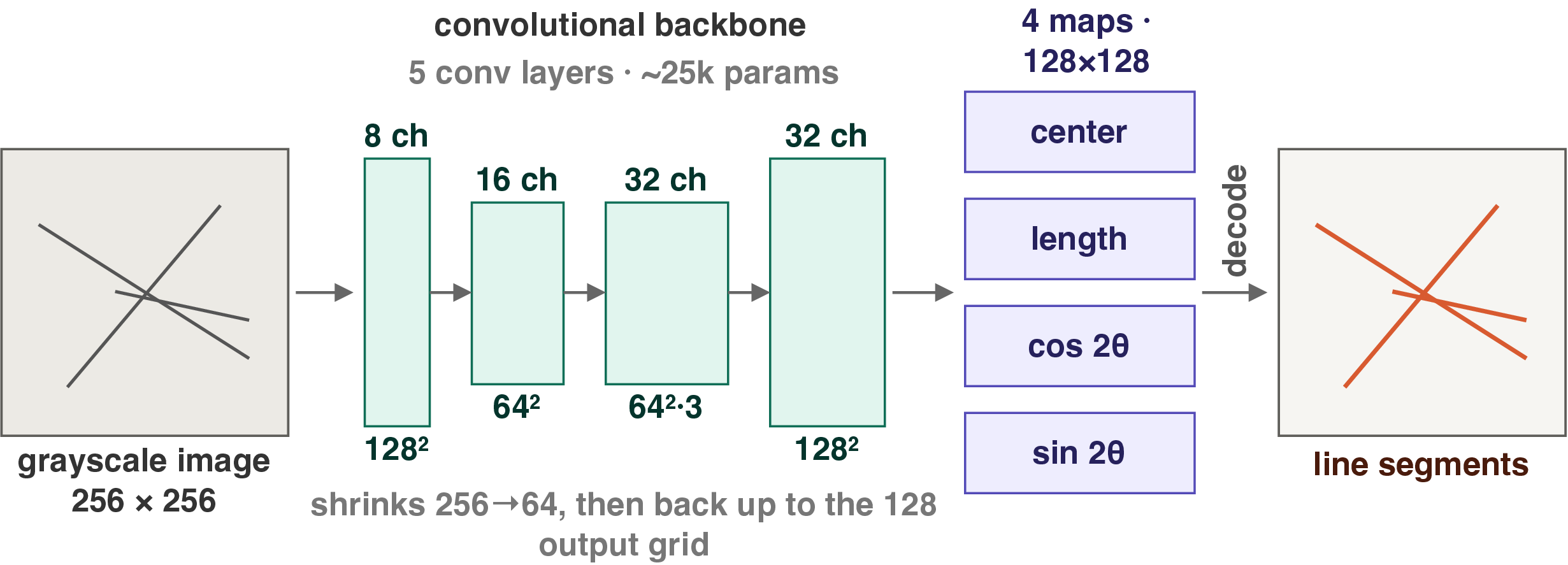
All three output heads share a common compact backbone designed to minimize activation memory while preserving sufficient spatial resolution for accurate line localization. The architecture (Fig. 2) consists of:
A strided fully-convolutional encoder with five convolutional layers, channel widths \(8 \to 16 \to 32 \to 32 \to 32\), and stride-2 downsampling that reduces the input resolution from \(256\times256\) to \(64\times64\).
A \(1\times1\) convolutional reduction layer that projects features to a compact representation.
A nearest-neighbor upsampling layer that restores the spatial resolution to \(128\times128\).
A \(3\times3\) output head that produces the final prediction maps (center confidence, length, and orientation for F-Clip; center and displacements for endpoint representation; or a single heatmap).
The total parameter count is approximately \(25\)k at the smallest width. Section 4.4 demonstrates that parameter capacity is not the primary bottleneck in this regime; rather, input resolution and activation memory constrain performance.
2.3 Quantization for MCU Deployment↩︎

To fit the model within microcontroller SRAM and use optimized integer inference kernels such as CMSIS-NN [26], we quantize weights and activations to integer precision. We adopt per-tensor symmetric quantization, implemented with fake-quantization in the forward pass and the straight-through estimator (STE) for gradient propagation during backpropagation [17], [18].
For a weight tensor \(w\) and target bit-width \(b\), the quantization scale is: \[s = \frac{\max|w|}{2^{b-1} - 1}\] The quantized weight is computed as: \[\hat{w} = s \cdot \operatorname{round}\left(\frac{w}{s}\right)\] This operation snaps continuous values onto a discrete grid of \(2^b\) levels. As illustrated in Fig. 3, 8-bit quantization provides 256 levels, offering fine granularity, while 4-bit quantization reduces this to only 16 levels, introducing substantial rounding error.
We evaluate two quantization strategies:
Post-training quantization (PTQ): The model is first trained in full precision, then weights and activations are quantized once using a small calibration set. This is computationally efficient but can suffer from accuracy degradation, particularly at low bit-widths.
Quantization-aware training (QAT): The quantization operation is simulated during training, allowing the model to learn weights that are robust to quantization error. While more expensive, QAT often recovers some of the accuracy lost in PTQ.
Our deployed model uses int8 quantization with QAT, achieving performance comparable to full precision as shown in Section 4.2. We also investigate 4-bit quantization to understand the limits of aggressive compression, revealing that angle regression is particularly sensitive to bit-width reduction.
2.4 Training Pipeline and Deployment Flow↩︎
Training is performed entirely off-device on a GPU workstation; the microcontroller executes only int8 inference. This train-off / infer-on split is the defining premise of our deployment strategy and is common practice in TinyML systems.
The training pipeline proceeds as follows:
A \(256\times256\) grayscale image is fed into the backbone.
The network produces prediction maps (center, length, \(\cos 2\theta\), \(\sin 2\theta\) for F-Clip) on a \(128\times128\) grid.
Loss is computed against ground-truth segments encoded in the same representation, using a combination of binary cross-entropy for center confidence and smooth L1 loss for geometric attributes.
For QAT, quantization simulation is enabled during training with STE gradient propagation.
For deployment, the trained model is exported through X-CUBE-AI, STMicroelectronics’ neural network inference library for STM32 microcontrollers. The export process generates optimized C code that runs on the Arm Cortex-M7 core, using CMSIS-NN for efficient integer arithmetic. The inference pipeline on the MCU (Fig. 4) consists of:
Input image capture (grayscale, \(256\times256\)).
int8 inference through the quantized network.
Decoding of output maps into line segments (center detection, length and angle extraction, endpoint computation).
Optional post-processing: Line-of-Interest verification and non-maximum suppression.
The entire inference pipeline is designed to operate within the 320 KB SRAM budget of the STM32F746, with peak activation memory as the primary constraint rather than parameter storage.

3 Experimental Setup↩︎
3.0.0.1 Dataset and metric
We train and evaluate on the ShanghaiTech Wireframe benchmark [8] (5,000 training and 462 held-out evaluation images, \(\sim\)74 segments per image). Accuracy is structural average precision \(\mathrm{sAP}^{t}\) at squared-endpoint-distance thresholds \(t\in\{5,10,15\}\) in the \(128^2\) output space; we headline \(\mathrm{sAP}^{10}\). For comparability with the FPGA predecessor [25] we also reference its Q1 (coverage) and Q2 (noise-suppression) measures.
3.0.0.2 Implementation
Table 2 lists the training configuration. Training is in PyTorch on a GPU; versions v1–v6 of the design search [27] share the backbone of Section 2. All models are trained for 300 epochs with a batch size of 32, using the Adam optimizer and a cosine annealing learning rate schedule starting from \(10^{-3}\). Data augmentation is limited to random horizontal and vertical flips. The loss function combines binary cross-entropy for center classification with smooth L1 loss for length and angle regression, weighted by a factor of 2.0 for the geometric terms and masked to ground-truth segment locations. We evaluate both PTQ and QAT at 8 and 4 bits.
| Setting | Value |
|---|---|
| Input \(\to\) output resolution | \(256\times256 \to 128\times128\) |
| Backbone channels | \(8\!\to\!16\!\to\!32\!\to\!32\!\to\!32\) (\(\sim\)25k params) |
| Output head | center, length, \(\cos2\theta\), \(\sin2\theta\) |
| Epochs / batch | 300 / 32 |
| Optimizer / LR | Adam / \(1\times10^{-3}\), cosine schedule |
| Augmentation | horizontal \(+\) vertical flip |
| Loss | BCE(center) \(+\,2.0\times\) L1(length, angle), masked |
| Quantization | per-tensor symmetric; PTQ and QAT |
4 Results↩︎
4.1 Representation Comparison: The Climb↩︎
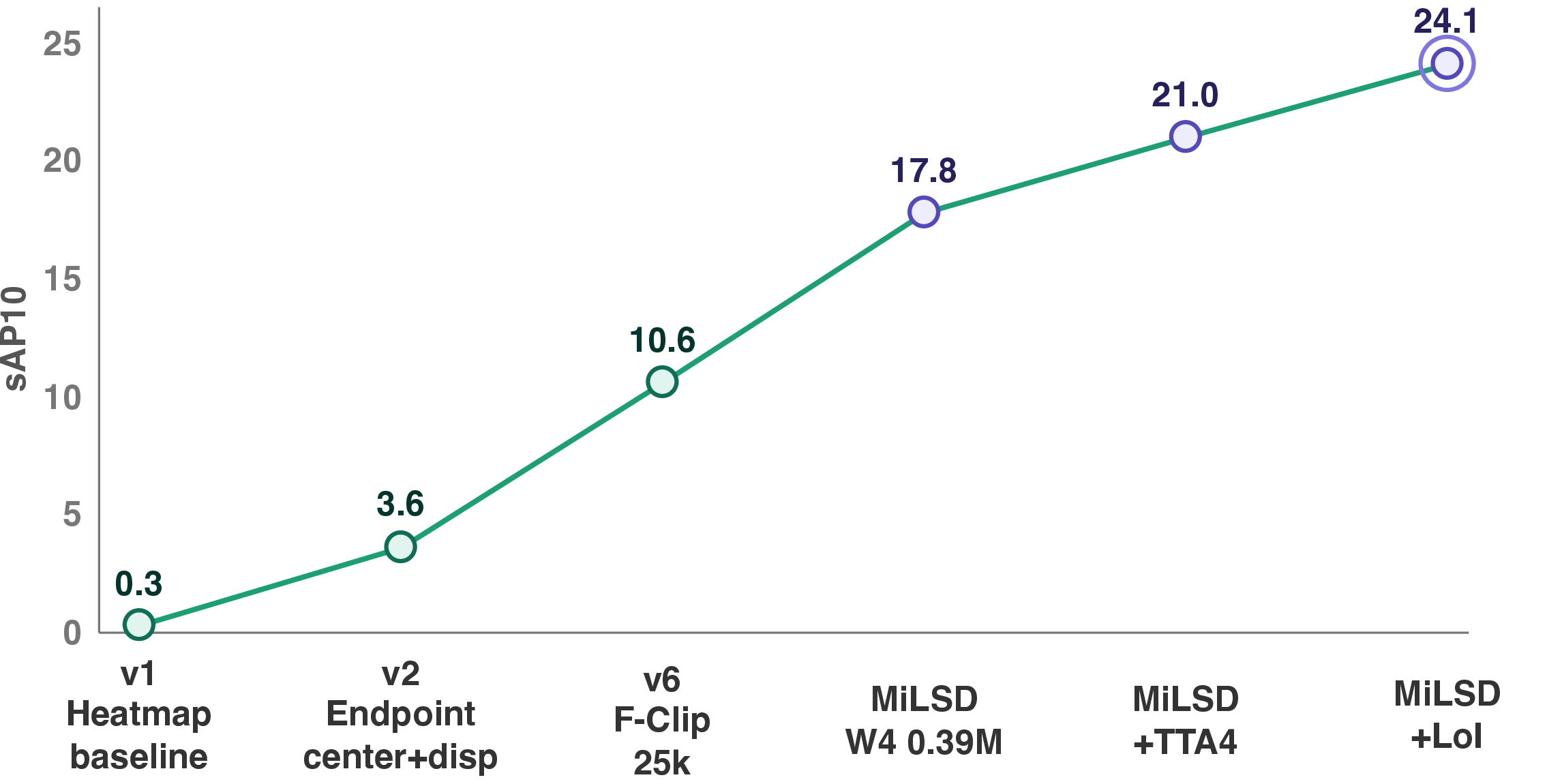
Fig. 5 traces the evolution of \(\mathrm{sAP}^{10}\) across the successive versions v1–v6 of our design search, providing a step-by-step account of how accuracy accumulates as each design choice is introduced. At the lowest rung of this progression, the heatmap baseline proves fundamentally inadequate for producing clean, discrete segments, registering only \(\mathrm{sAP}^{10}=0.3\). Endpoint regression constitutes the first formulation capable of yielding a meaningful structural score, reaching \(\mathrm{sAP}^{10}=3.6\), yet it remains limited in its ability to recover coherent geometry. The decisive inflection occurs with the adoption of the F-Clip representation, which at the identical 25k-parameter budget more than doubles performance to \(\mathrm{sAP}^{10}=7.2\), establishing that the output encoding itself, rather than model size, is the dominant factor at this scale. Subsequent refinements complete the climb in a more incremental fashion: aligning the output grid with the label resolution at \(256\) px input lifts accuracy to \(8.6\); incorporating the full training set of 5,000 images together with flip augmentation raises it further to \(9.3\); and extending the training schedule to 300 epochs yields the final deployed score of \(\mathrm{sAP}^{10}=10.6\). Taken together, these results demonstrate unambiguously that the largest gains originate from the choice of representation, not from additional capacity. This finding carries particular significance for microcontroller-scale design: a geometric encoding that explicitly parameterizes each segment by its center, length, and orientation equips even a 25k-parameter network with sufficient inductive structure to learn meaningful segment hypotheses, whereas the heatmap and endpoint alternatives remain unable to assemble coherent geometric predictions under the same severe parameter constraint.
4.2 Quantization↩︎
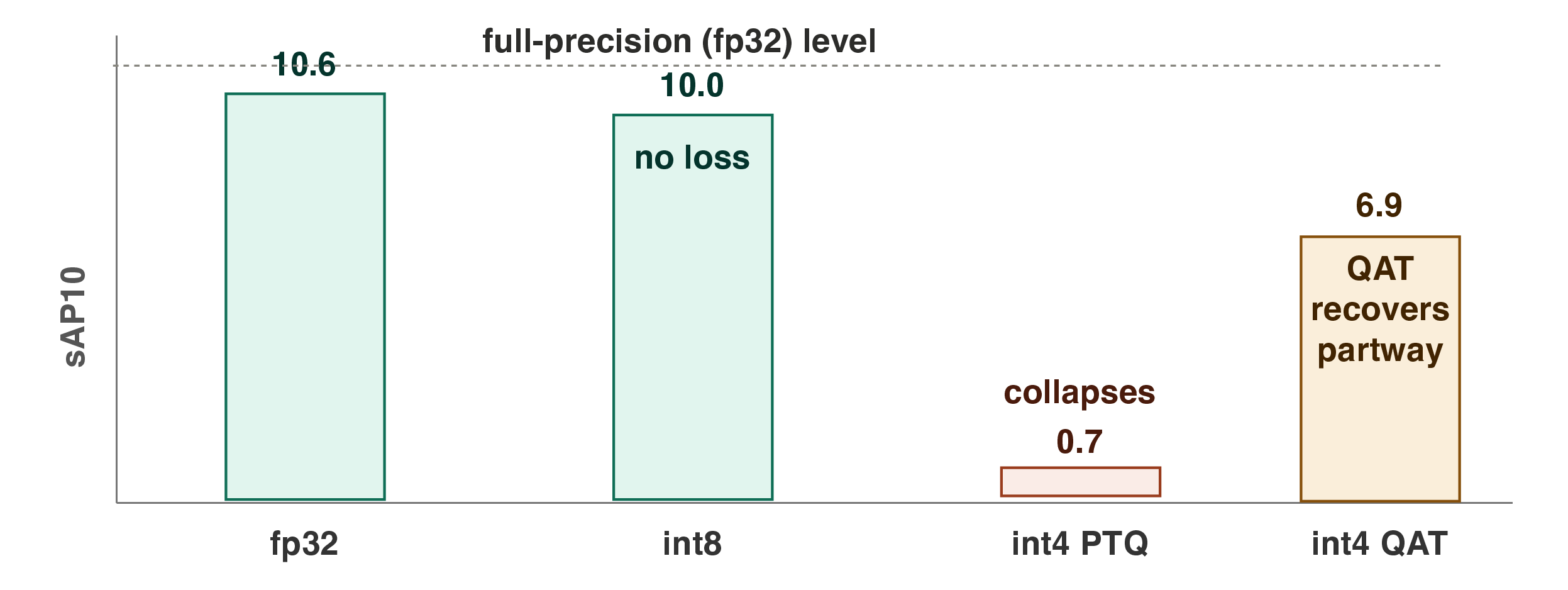
Fig. 6 and Table 3 present the results of our systematic quantization study, evaluated across the three principal output representations corresponding to versions v1, v2, and v6 of the design search. For the deployed F-Clip model, the transition from full-precision fp32 inference to 8-bit integer quantization incurs a degradation of only \(0.6\) \(\mathrm{sAP}^{10}\) points (\(10.6\rightarrow10.0\)), indicating that int8 arithmetic is sufficient for on-device deployment with negligible impact on structural accuracy. By contrast, post-training quantization at 4 bits proves catastrophic, collapsing performance to \(\mathrm{sAP}^{10}=0.7\); quantization-aware training partially mitigates this failure, recovering the score to \(6.9\), which corresponds to approximately \(60\%\) of the int4-induced gap relative to the fp32 baseline. Inspection of the per-head errors reveals that the degradation is concentrated almost entirely in the \((\cos2\theta,\sin2\theta)\) angle regression branch, whose inherently narrow dynamic range is poorly served by the coarse 4-bit quantization grid. On this basis, the deployed model adopts int8 throughout. More broadly, these results suggest that pushing quantization beyond 8 bits is unlikely to remain viable for geometric regression heads of this kind without substantial architectural or training modifications.
| Representation | fp32 | int8 | int4 PTQ | int4 QAT |
|---|---|---|---|---|
| Heatmap (v1)\(^{*}\) | 0.3 | 0.3 | 0.3 | n/a |
| Endpoint (v2) | 3.6 | 3.6 | \(\sim\)0.3 | fragile |
| F-Clip (v6, deployed) | 10.6 | 10.0 | 0.7 | 6.9 |
\(^{*}\)Heatmap is not built for sAP; on its own terms Q2\(=0.86\), recall\(=0.44\).
4.3 Resolution–Memory Trade-off↩︎
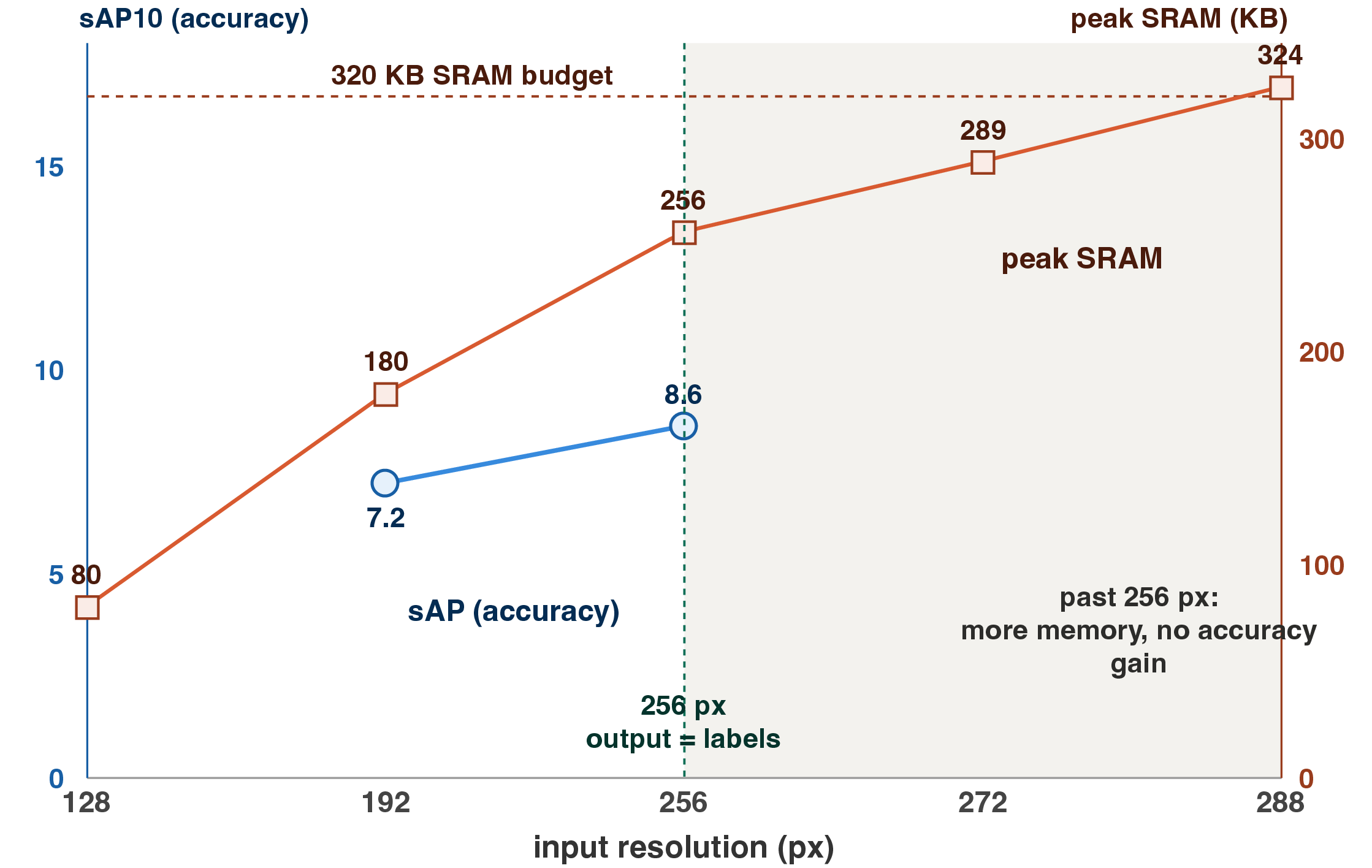
Fig. 7 plots both \(\mathrm{sAP}^{10}\) and peak SRAM consumption as functions of input resolution, enabling a joint assessment of the accuracy–memory trade-off that governs operating-point selection on resource-constrained hardware. The chosen configuration of \(256\) px input is selected at the point where the \(128\times128\) output grid aligns with the native label resolution, and where peak SRAM remains within the 320 KB ceiling imposed by the STM32F746. This analysis reveals a pronounced and interpretable trade-off: as input resolution increases, structural accuracy improves steadily until the output grid reaches parity with the label resolution, at which point further resolution gains yield diminishing or negligible returns. Beyond this saturation point, peak SRAM continues to grow without a commensurate accuracy benefit. The \(256\) px operating point therefore represents the optimal balance between detection quality and memory footprint for the F746 deployment target.
4.4 Capacity and Overfitting↩︎
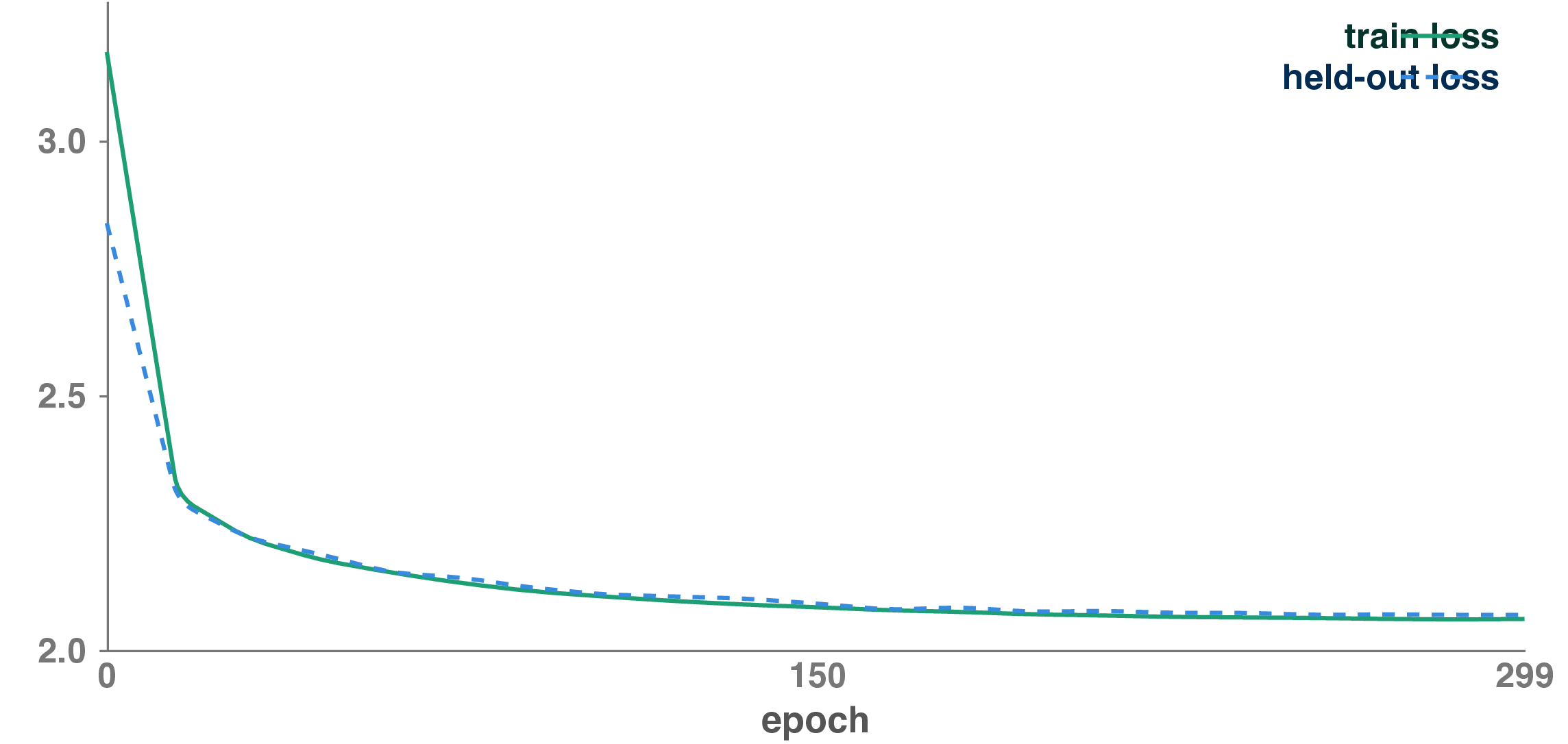
To test whether the 25k-parameter backbone is capacity-limited, we swept backbone width through three operating points (\(\sim\)25k, \(\sim\)98k, and \(\sim\)209k parameters) while holding all other training settings fixed, and recorded the held-out loss floor at convergence. The result is nearly flat: the smallest model settles at \(1.74\), while the intermediate and largest variants both reach \(1.73\); an eightfold increase in parameters yields only a \(0.01\) reduction in held-out loss. This pattern is consistent with the capacity-gap effect documented in the knowledge-distillation literature [28], and implies limited headroom for naive distillation-based improvement at this scale. The flatness further suggests that the model is already operating near the information-theoretic limit imposed by the dataset and the chosen input resolution, such that additional parameters are unlikely to translate into measurable gains in structural accuracy. Complementing this capacity analysis, Fig. 8 plots the training and held-out loss trajectories over the full 300-epoch schedule. The two curves remain closely aligned throughout training, converging to a final gap of approximately \(0.01\), indicating the absence of overfitting despite the severely constrained 25k-parameter architecture and the modest size of the training set. Together, these observations support the conclusion that the fixed small-width design is both memory-efficient and well-regularized by its architectural constraints.
4.5 Comparison with Prior Work↩︎
![Figure 9: Accuracy vs.parameter budget on the Wireframe benchmark (log-scale x). Our two operating points sit at the extreme low-resource end: the 25k-parameter F-Clip model on the STM32F746 (\mathrm{sAP}^{10}=10.6) and MiLSD on the STM32H7 (0.39 M parameters, \mathrm{sAP}^{10}=24.1, purple). Related learned detectors use 24\times to 1{,}600\times more parameters and assume mobile or GPU compute; their figures are from the respective papers (Table 4) [3]–[6], [8], [9], [21].](/article/2607.06600/Figs/fig_accuracy_memory.png "fig:")
Table 4 and Fig. 9 jointly situate our two operating points within the broader accuracy–resource frontier of the learned line-segment detection literature. At the low-resource end of this range, the 25k-parameter F746 model achieves \(\mathrm{sAP}^{10}=10.6\) within a 0.25 MB activation footprint, while MiLSD (Section 5) extends this capability to \(\mathrm{sAP}^{10}=24.1\) under the expanded 1 MB SRAM budget of the STM32H7. In absolute accuracy terms, both models remain substantially below the performance of contemporary transformer-era parsers, including DT-LSD at \(71.7\) [29] and LINEA at \(65.0\)–\(67.9\) [30], as well as compact GPU-oriented designs such as EM-LSD, which attains \(63.2\) with \(1.1\) M parameters [31]. This disparity is an expected consequence of operating in a memory regime where peak SRAM is measured in kilobytes rather than megabytes. On the resource axis, however, our position is distinctive: Table 4 lists no other learned detector with an affirmative On MCU? entry or an accompanying int8/int4 quantization study. To our knowledge, this is the first learned line-segment detector designed and evaluated under sub-megabyte MCU SRAM budgets, occupying a previously empty region between high-accuracy GPU-based parsers and classical lightweight detectors.
4.6 Qualitative Results↩︎
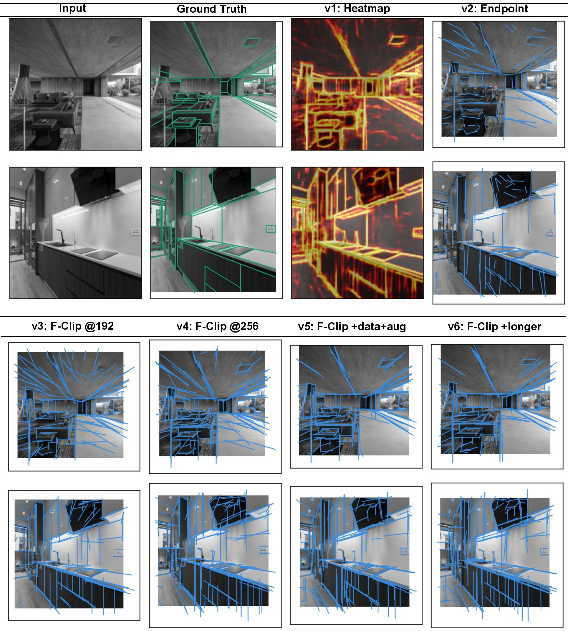
Fig. 10 provides a qualitative side-by-side comparison of versions v1 through v6 on two representative Wireframe-val images [27], offering visual corroboration of the quantitative trends reported above. In the heatmap formulation (v1), predictions remain densely distributed across the image without resolving into discrete, well-formed segments. Endpoint regression (v2) produces scattered short segments that fail to reconstruct the underlying room structure. Beginning with F-Clip at v3, the detections progressively recover coherent architectural geometry, a visual pattern that directly mirrors the quantitative \(\mathrm{sAP}^{10}\) jump at v3 (\(3.6\rightarrow7.2\)) and the more incremental refinement observed across v3–v6 (\(7.2\rightarrow10.6\)). The qualitative contrast is visually striking: F-Clip yields coherent, well-localized segments that align closely with salient architectural edges, whereas the heatmap and endpoint alternatives continue to produce noisy, fragmented, or incomplete detections that lack geometric consistency.
5 MiLSD: Verification-Augmented Detection on the STM32H7↩︎

The 320 KB SRAM budget of the STM32F746 imposes a hard ceiling on the detector developed in Section 2, restricting it to approximately 25k parameters and a correspondingly minimal activation footprint. A larger yet still microcontroller-class platform, the STM32H7, which provides 1 MB of SRAM and is executed via CMSIS-NN [26] on a Cortex-M7 core, affords sufficient headroom to accommodate both a more capable backbone and a substantially richer inference pipeline. We designate the resulting system MiLSD (Micro Line-Segment Detector). MiLSD preserves the F-Clip center–length–angle output representation [5] (Section 2.1) introduced earlier and extends it along two complementary axes: first, a capacity-scaled int8 backbone whose activation arena is deliberately sized to approach, but not exceed, the 1 MB SRAM budget; and second, a sequence of inference-time refinement stages, comprising sub-pixel decoding, test-time augmentation, and a learned verification head, each of which contributes additional accuracy without increasing the size of the trained network. The complete pipeline is illustrated in Fig. 11. In contrast to the F746 model, whose performance is bounded by its severely constrained 25k-parameter budget, MiLSD exploits the expanded memory envelope to scale model capacity while preserving a lightweight, inference-efficient pipeline appropriate for real-time embedded deployment.
5.1 Capacity-Scaled Backbone↩︎
With eight times the SRAM of the F746, the backbone width is increased until the int8 activation arena approaches, but does not exceed, 1 MB, yielding a approximately 0.39 M-parameter model (peak arena approximately 1 MB at 256 px input; a 0.7 MB fallback configuration is also retained for devices with tighter memory). Trained as in Section 2 for 300 epochs, this model attains \(\mathrm{sAP}^{10}=17.8\) on Wireframe-val, versus \(10.6\) for the 25k F746 model, confirming that, beyond the extreme F746 regime, capacity is a genuine lever. This 68% relative improvement demonstrates that the additional parameters are effectively utilized when the memory budget permits, validating our decision to scale the backbone for the H7 platform.
5.2 Sub-Pixel Decoding and Test-Time Augmentation↩︎
The center peaks are refined to sub-pixel accuracy by a one-dimensional parabolic fit over each peak’s neighbourhood, directly targeting the endpoint precision that structural AP rewards (\(\mathrm{sAP}^{10}: 17.8 \rightarrow 18.1\)). This refinement is particularly beneficial for structural AP, which penalizes endpoint localization errors quadratically. Averaging the predicted maps over the image and its horizontal, vertical, and diagonal flips (test-time augmentation, TTA) further improves robustness (\(\mathrm{sAP}^{10}: 18.1 \rightarrow 21.0\)), a gain of nearly 3 points from the four-view ensemble. TTA multiplies inference latency by the number of views but reuses the same activation arena, so it does not raise peak memory, making it a memory-free accuracy boost at the cost of increased latency.
5.3 Line-of-Interest Verification Head↩︎
The largest gain comes from a trained verifier in the spirit of L-CNN [3] and HAWP [4], scaled to the microcontroller. With the backbone frozen, a small multilayer perceptron takes, for each candidate segment, features bilinearly pooled at 32 points along the line from the backbone feature map and the output maps, together with a short geometric descriptor, and predicts a verification score (real vs.spurious), trained with one-to-one matched labels. Re-ranking by verification \(\times\) center score reaches the MiLSD row of Table 5. The decode and post-filtering design were obtained by analyzing the inference stages of the principal wireframe parsers [3]–[5], [32], [33]; across that study, weight-free post-processing saturates near \(\mathrm{sAP}^{10}=21\), and only the trained verifier advances beyond it, contributing an additional 3.1 points to reach 24.1.
| Configuration | |||
|---|---|---|---|
| Trained model (sub-pixel decode) | 12.1 | 18.1 | 21.2 |
| + test-time augmentation (\(\times4\)) | 15.1 | 21.0 | 24.0 |
| + LoI verification (MiLSD) | 16.0 | 24.1 | 27.9 |
| Oracle (perfect verifier) | 24.1 | 37.4 | 40.0 |
The oracle row (\(\mathrm{sAP}^{10}=37.4\)) bounds what the candidate set can deliver; the LoI head recovers about 55% of the gap from TTA. The remainder reflects unannotated image edges and recall limits; junction-based candidate generation [3] could help but exceeds the 1 MB budget.
5.4 Qualitative Results↩︎
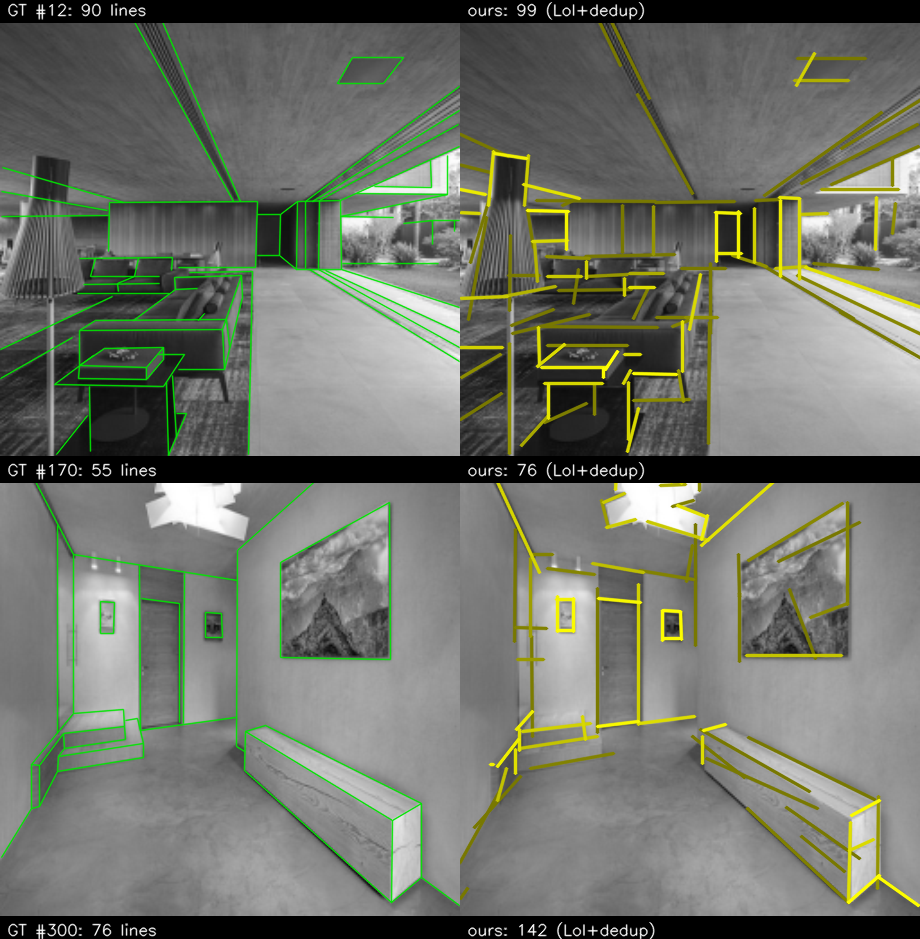
Fig. 12 shows MiLSD on held-out scenes. The detector is complete on the salient structure (cabinetry, counters, window mullions, and architectural edges are recovered at correct orientation and length). The dense scene of example 2 illustrates the verifier suppressing the redundant ridge detections that a raw center-heatmap emits, demonstrating the effectiveness of the learned verification head. Example 3 shows that the remaining stray predictions are real but unannotated edges (reflections, texture seams), consistent with the oracle analysis above, which identified that many false positives are actually unlabeled ground-truth edges. These qualitative results validate that MiLSD achieves its accuracy gains through meaningful structural understanding rather than overfitting to the training set.
5.5 Deployment Budget↩︎
The SRAM ceiling is set by the backbone’s int8 activation arena (approximately 1 MB); the LoI head’s pooled feature (\(<\)0.5 MB) fits within that peak and TTA reuses it, so neither raises it. Weights total approximately 0.54 MB (backbone plus head), well within flash. Latency is dominated by the int8 convolutions and scales with the number of TTA views; the LoI head adds a small per-line cost. On-device arena and latency must be confirmed with ST Edge AI [34]; the figures here are software-measured. The memory-efficient design ensures that all inference stages operate within the 1 MB SRAM budget, making MiLSD deployable on the STM32H7 without requiring external memory. Source code is released for reproducibility [35].
6 Conclusion↩︎
This paper presented MiLSD, a line-segment detector explicitly designed for microcontroller-scale memory, alongside a systematic study of the accuracy–resource trade-off under extreme memory constraints. We compared three output representations and found that the F-Clip center-with-length-and-angle encoding learns most effectively at small model sizes, achieving \(\mathrm{sAP}^{10}=10.6\) with only 25k parameters. Our quantization study revealed that 8-bit weights preserve full-precision accuracy, while 4-bit quantization collapses, particularly in the \((\cos2\theta,\sin2\theta)\) angle regression, with quantization-aware training recovering only part of the loss. By scaling the backbone to a 1 MB activation budget and adding inference-time enhancements including sub-pixel decoding, test-time augmentation, and a Line-of-Interest verification head, MiLSD improves \(\mathrm{sAP}^{10}\) from \(10.6\) at 0.25 MB to \(24.1\) within 1 MB on the ShanghaiTech Wireframe benchmark.
To our knowledge, no prior work characterizes the joint trade-off among representation choice, quantization bit-width, and on-device post-processing at this memory scale. F-Clip wins at int8 but its angle head is int4-fragile, whereas heatmaps tolerate lower precision yet require an external linker, a finding that informs future TinyML geometric-vision designs. As expected, Wireframe accuracy remains far below GPU-class parsers given the SRAM envelope we target; that gap is inherent to the memory regime rather than a limitation we aim to overcome.
Parsa Hassani Shariat Panahi received his B.Sc. degree in Computer Engineering from Azad University South Tehran Branch, Tehran, Iran, and the M.Sc. degree in Computer Engineering - Computer Networks from Iran University of Science and Technology, Tehran, Iran. His research interests include cellular networks, QoE assessment, telecommunication networks, wireless communication, and machine learning. He can be reached at parsa_hassani@comp.iust.ac.ir.
Amir Hossein Jalilvand received his B.Sc. degree in Computer Engineering from Bu-Ali Sina University, Hamadan, Iran, and the M.Sc. degree in Computer Engineering - Computer Architecture from Iran University of Science and Technology, Tehran, Iran. He is currently pursuing his Ph.D. in Computer Engineering. His research interests include cellular networks, stochastic and unary computing, computer architecture, fuzzy logic, and machine learning. Mr. Jalilvand has authored several publications in these fields. He can be reached at jalilvand_a@comp.iust.ac.ir.
M. Hassan Najafi received his Ph.D. in electrical and electronics engineering from the University of Minnesota-Twin Cities, Minneapolis, MN, USA, in 2018. He is currently an Associate Professor at the Electrical, Computer, and Systems Engineering Department at Case Western Reserve University. His research interests include stochastic and approximate computing, unary processing, in-memory computing, and hyperdimensional computing. He has authored/coauthored more than 120 peer-reviewed papers and has been granted 12 U.S. patents with more pending. Dr. Najafi received the NSF CAREER Award in 2024, the Best Paper Award at GLSVLSI’23 and ICCD’17, and the 2018 EDAA Outstanding Dissertation Award. Dr. Najafi is a senior member of IEEE and a senior member of the U.S. National Academy of Inventors (NAI). He can be reached at najafi@case.edu.
References↩︎
\(^\pi\)School of Computer Engineering, Iran University of Science and Technology, Tehran, Iran
\(^+\)Electrical, Computer, and Systems Engineering Department, Case Western Reserve University, OH, USA↩︎