Graph Convolutional Attention: A Spectral Perspective on Graph Denoising and Diffusion
July 07, 2026
Abstract
Denoising graphs is a fundamental problem in graph learning and the core operation of graph diffusion models. Attention-based architectures like graph transformers have recently shown promise in denoising graphs. However, our principled understanding of attention-based graph denoising remains limited, making it unclear whether standard attention is the right mechanism for this task. Here we show that, under a denoising objective, linear attention is suboptimal and can only learn an average spectral denoising filter over the training distribution. This creates a fundamental limitation as graphs often vary spectrally across the distribution. To overcome this limitation, we introduce Spectral Attention, which directly utilizes the input graph spectrum and provably outperforms linear attention by a margin governed by the spectral diversity of the distribution. We then derive Graph Convolutional Attention (GCA), a practical and permutation-equivariant realization of this idea that implements spectral denoising through graph-filtered queries and keys. For stochastic block models, GCA provably matches the idealized Spectral Attention mechanism. We further show that the softmax operation, that follows the attention, provides additional denoising by approximately projecting noisy eigenvectors onto the clean eigenspace. Empirically, replacing linear attention with GCA consistently improves graph denoising and diffusion on synthetic and real datasets, with gains strongly correlated with spectral diversity. In DiGress, GCA matches standard graph-transformer performance without computing expensive structural features, and when combined with the recently proposed PEARL positional encodings, avoids explicit eigendecomposition computations resulting in faster inference without degrading quality. The code can be found here: github.com/shervinkhalafi/graph_conv_att
1 Introduction↩︎
Denoising is a fundamental problem in machine learning [1], both in its own right and as the central learning primitive behind denoising diffusion models [2], [3]. Graph denoising introduces a unique challenge: the object to be denoised is not merely a signal on a known domain, but the domain itself. In image and audio denoising, the underlying grid or temporal axis is fixed, so models can exploit geometry through convolutions [4]. In graphs, by contrast, the geometry and spectral frequency is corrupted and must itself be recovered. Classical approaches address graph denoising through regularized optimization [5], [6], but the parametric perspective has received comparatively little attention. Interest has grown recently, driven by graph diffusion models [7], [8], where the dominant approach is graph transformers that take the eigenvectors of the graph, and optionally additional structural features, as input. Yet a theoretical understanding of how such parametric models learn to denoise graphs remains limited. In this work, we aim to provide insight into the mechanisms underlying parametric graph denoising through theoretical analysis.
We proceed in four steps. First, we (i) analyze linear attention, the outer product of linear query-key projections, as it underlies every attention-based graph denoiser. We show it learns an average of the spectral properties across the graph distribution, which is suboptimal when those spectra vary. To address this sub-optimality, we (ii) introduce and analyze the spectral attention, an abstract class in which the attention mechanism depends arbitrarily on the input eigenvalues. The loss with respect to spectral attention is strictly smaller than that of linear attention, and the gap depends on the concept of spectral diversity, i.e., how diverse the spectra are across the distribution. Spectral attention, however, is abstract and in general not permutation equivariant. To turn the insight into something usable, we (iii) introduce graph convolutional attention (GCA), in which the attention pattern is a pointwise function of the eigenvalues. This makes the mechanism permutation equivariant and expressible as a graph convolutional filter. For asymptotically large Stochastic Block Models (SBMs), we show that under suitable conditions GCA matches spectral attention and therefore strictly improves on linear attention. Finally, we (iv) analyze the nonlinearity, typically a softmax, that follows linear attention. We show that once the clean eigenvalues are known, e.g., recovered by GCA, the softmax denoises the eigenvectors by acting like an approximate projection onto the subspace spanned by the clean eigenvectors, which provably reduces noise.
Experimentally, across real and synthetic datasets, a graph transformer using GCA in place of the standard query-key projections outperforms the standard graph transformer at denoising, and the per-dataset improvement correlates strongly with a surrogate of the spectral diversity metric, validating the theory. For diffusion models, GCA improves training loss and, on many datasets, sample quality both qualitatively and under standard metrics. Finally, drop-in augmentation of DiGress with GCA + R-PEARL[9] is competitive with the standard DiGress without any hyperparameter tuning, slightly improving on some MMDs without its usual expensive to compute spectral features.
We summarize our contributions as follows:
Theoretical analysis of attention-based denoising. We show linear attention only learns an average of spectral properties over the graph distribution, which is suboptimal when graphs have varying spectra. We introduce spectral attention, and show that its improvement over linear attention is captured by the spectral diversity of the graph distribution.
Graph Convolutional Attention (GCA). Motivated by the analysis, we propose GCA, where the attention pattern can be expressed as a graph convolutional filter, making it permutation equivariant. For asymptotically large SBMs, we show GCA matches the optimal loss of spectral attention, and thus strictly outperforms linear attention.
Role of the softmax. In the SBM setting, we show that softmax can further improve the denoising of graph by comparing it to a projection of the noisy eigenvectors onto the eigenbasis spanned by the clean eigenvectors.
Empirical validation. Across real and synthetic datasets, replacing standard query-key projections with GCA consistently improves denoising, and the per-dataset gain correlates with a surrogate of our spectral diversity metric, directly validating the theory. The gains transfer to discrete diffusion: GCA yields lower training loss and better samples.
Implications for modern diffusion models. Plugging GCA into DiGress we observe that we can match DiGress performance with hand-crafted features while avoiding their cost. Combined with R-PEARL, it can even sidestep eigenvector computation entirely leading to a reduction in training and inference time on larger graphs.
1.1 Literature review↩︎
1.1.0.1 Graph denoising.
Existing graph denoising methods can be broadly divided into optimization-based and learned approaches. The former recover a clean graph by solving an inverse problem regularized with structural priors such as edge-error models [5], [10], spectral consistency [6], [11], [12], or low-rank, sparse, and smooth graph structure [13]–[15]. The latter replace instance-wise optimization with a parametric denoiser, either as a preprocessing or jointly trained module for downstream GNNs [16]–[18], or as the core component of diffusion and flow-based generative models that iteratively remove graph corruption [7], [8], [19]. Overall, prior work spans from hand-crafted regularization to fully learned graph restoration, but most methods are not designed to explicitly exploit spectral structure within the denoising mechanism itself.
1.1.0.2 Spectral attention.
A parallel line of work incorporates graph spectral information into Transformer architectures. Early methods use Laplacian eigenvectors or eigenvalues as spectral features or positional encodings for attention-based models [20]–[23], while later approaches address eigenvector ambiguities through invariant spectral encoders such as SignNet and BasisNet [24]. More recent models integrate spectral structure directly into the attention mechanism or the learned operator. GIST reweights attention using inner products of random filtered spectral features [25], whereas Specformer, PolyFormer, and Eigenformer use Transformer blocks to parametrize spectral filters using attention [26]–[28]. These works show that spectral information can be embedded into attention in several ways, but they are mainly aimed at representation learning and prediction rather than graph denoising.
2 Denoising Graphs with a Linear Model↩︎
2.0.0.1 Problem Setup.
We start with the graph denoising problem as it is fundamental to graph diffusion. In particular, the next two sections analyze how attention-based neural networks perform denoising from a spectral perspective. We first show that the linear part of the network can learn to denoise the eigenvalues of a noisy graph. Then, in Section 3, we show that the nonlinearities help remove noise from the eigenvectors. We consider unweighted, undirected graphs \(\mathcal{G}\) sampled from a distribution over graphs which we denote \(\mathcal{D}_{\mathcal{G}}\). For a given graph \(\mathcal{G}\), we denote by \(A \in \mathbb{R}^{n \times n}\) the symmetric adjacency matrix. Denote the noisy adjacency \(\widetilde{A} = A + \mathcal{E}\), where \(\mathcal{E} \in \mathbb{R}^{n \times n}\) is a symmetric noise matrix sampled from a noise distribution. We note that depending on the noising method this distribution could depend on the input graph for example when flipping edges in an unweighted graph, or it could be independent e.g., Gaussian noise. We write the eigendecomposition of the adjacency as \(A = U \Lambda U^\top\), and that of the noisy adjacency as \(\widetilde{A} = \widetilde{U} \widetilde{\Lambda} \widetilde{U}^\top\).
2.1 Using Eigenvalue Information Improves Denoising.↩︎
Consider an arbitrary denoising function \(f(\cdot):\mathbb{R}^{n \times n}\rightarrow \mathbb{R}^{n \times n}\) that takes the noisy adjacency as input and returns a prediction of the denoised graph. We define the following loss functional characterizing the denoising capability of \(f\) over different graphs and noise samples from the distribution: \[\ell(f) = \,\,\mathbb{E}_{A,\,\mathcal{E}} \left\| f(\widetilde{A}) - A \right\|_F^2\]
A common candidate for implementing the denoising map is attention [8], [29]. For a sequence of \(d\)-dimensional input tokens \(X \in \reals^{n \times d}\), standard attention computes \[g_{\text{\normalfont{Att}}}(X) = \text{softmax}(X W_Q W_K^\top X^\top) X W_V\] where \(W_Q \in \reals^{d \times d_k}\), \(W_K \in \reals^{d \times d_k}\), and \(W_V \in \reals^{d \times d_v}\) are learnable query, key, and value matrices, respectively. In graph denoising, attention-based estimators of the adjacency can be built as an outer product of representations [8]: \[\label{eq::graph95based95att} f(\widetilde{A})=g_{\mathrm{Att}}(\widetilde{U})g_{\mathrm{Att}}(\widetilde{U})^\top = \text{softmax}(\widetilde{U} W_Q W_K^\top \widetilde{U}^\top) \cdot \widetilde{U} W_V W_V^\top \widetilde{U}^\top \cdot \text{softmax}(\widetilde{U} W_Q W_K^\top \widetilde{U}^\top)^\top.\tag{1}\] In this view, attention acts on \(\widetilde{U}\) to recover a clean spectral representation of the underlying graph \(A\). We analyze this mechanism as a two-stage process. First, the score matrix \(\widetilde{U} W_Q W_K^\top \widetilde{U}^\top\) can be interpreted as a linear spectral estimator that seeks to recover a denoised graph with clean eigenvalues. Second, the \(\text{softmax}\) operation further denoises the noisy eigenvectors \(\widetilde{U}\) to approach the clean noiseless adjacency. To study the first step, in this section we restrict our focus to three classes of simplified graph-denoising maps:
Linear Attention: We define \(W = W_Q W_K^\top\) and consider the function class \(\mathcal{F}_{\text{LA}}\): \[\mathcal{F}_{\text{LA}} = \left\{ f(\widetilde{A}; W) = \widetilde{U} W \widetilde{U}^\top |\,\, W \in \mathbb{R}^{n \times n} \right\}\]
Spectral Attention: The broader class of functions \(\mathcal{F}_{\text{SA}}\) where the attention pattern can depend on the eigenvalues of the noisy input graph via any arbitrary function \(g(\cdot)\): \[\mathcal{F}_{\text{SA}} = \left\{ f(\widetilde{A}; g(\cdot)) = \widetilde{U} g(\widetilde{\Lambda}) \widetilde{U}^\top |\,\, g(\cdot):\mathbb{R}^{n} \rightarrow \mathbb{R}^{n \times n} \right\}\]
Graph Convolutional Attention: We consider the class of functions \(\mathcal{F}_{\text{GCA}}\) where the attention pattern is replaced by a function \(\eta(\cdot)\) acting point-wise on the eigenvalues of the graph: \[\label{eq:32GCA32definition} \mathcal{F}_{\text{GCA}} = \left\{ f(\widetilde{A}; \eta(\cdot)) = \widetilde{U} \eta(\widetilde{\Lambda}) \widetilde{U}^\top |\,\, \eta(\cdot):\mathbb{R} \rightarrow \mathbb{R} \right\},\tag{2}\] where, with a slight abuse of notation, \(\eta(\widetilde{\Lambda})\) denotes the pointwise application of \(\eta\) to the entries of the diagonal matrix \(\widetilde{\Lambda}\).
Note that the linear attention model is in general not permutation equivariant, due to the non-uniqueness of the eigenvectors. Similarly, the spectral attention model is also in general not permutation equivariant since \(\mathcal{F}_{\text{LA}} \subset \mathcal{F}_{\text{SA}}\). The graph convolutional attention model, however, is permutation equivariant as it can be written as \(f(\widetilde{A}; h(\cdot)) = \sum_{i = 1}^n h(\widetilde{\lambda}_i) v_i v_i^T\) which is a permutation equivariant aggregation of the eigenvectors each processed individually by the function \(h(\cdot)\).
Next, in Propositions 1, and 2 we characterize the minimum achievable loss for the linear and spectral attention classes respectively. The proofs can be found in Appendices 8.3, and 8.4.
Proposition 1. The minimum loss achievable with linear attention, \(\ell^\star_{\text{LA}} := \min_{f \in \mathcal{F}_{\text{LA}}} \ell(f)\), can be characterized as: \[\ell^\star_{\text{LA}} = \mathrm{tr}\left(\mathrm{Cov}(\mathrm{vec}(B))\right) + c,\,\] where \(B := \widetilde{U}^\top A \widetilde{U}\). Furthermore, the minimizer is given by \(f(\cdot\,; W^\star)\) where: \[W^\star = \mathbb{E}_{A,\,\mathcal{E}} [B]\]
Proposition 2. The minimum loss achievable with spectral attention, \(\ell^\star_{\text{SA}} := \min_{f \in \mathcal{F}_{\text{SA}}} \ell(f)\), can be characterized as: \[\ell^\star_{\text{SA}} = \mathrm{tr}\left(\mathrm{Cov}(\mathrm{vec}(B) \mid \widetilde{\Lambda})\right) + c\] where \(B := \widetilde{U}^\top A \widetilde{U}\). Furthermore, the minimizer is given by \(f(\cdot\,; g^\star)\) where: \[g^\star(\widetilde{\Lambda}) = \mathbb{E}_{A,\,\mathcal{E}}\!\left[B \;\middle|\; \widetilde{\Lambda}\right]\]
By the law of total variance, conditioning can only reduce variance, so \(\ell^\star_{\text{SA}}\) is going to be smaller or equal to \(\ell^\star_{\text{LA}}\). We formalize this in Theorem 1, proven in Appendix 8.5.
Theorem 1. The improvement in the minimum achievable loss by the spectral attention class compared to the linear attention class is given by: \[\label{eq:32spectral32diversity} \ell^\star_{\text{SA}} - \ell^\star_{\text{LA}} = \text{\normalfont{SD}}(\mathcal{D}_{\mathcal{G}}) := \mathbb{E}\left[\left\|\mathbb{E}[B \mid \widetilde{\Lambda}] - \mathbb{E}[B]\right\|_F^2\right] = \mathrm{tr}(\mathrm{Cov}(\mathbb{E}[\mathrm{vec}(B) \mid \widetilde{\Lambda}])),\qquad{(1)}\] where we define \(\text{\normalfont{SD}}(\mathcal{D}_{\mathcal{G}})\) as the ‘Spectral Diversity’ which depends on the graph data distribution and, implicitly, on the noise distribution.
Remark 1. The Spectral Diversity \(\text{\normalfont{SD}}(\mathcal{D}_{\mathcal{G}})\) essentially quantifies how much information we gain about the clean graph by observing the noisy spectrum. For more intuition on this, if we assume the noise is sufficiently small such that the noisy eigenvectors are close to the clean ones, then from ?? we can write \(\mathrm{tr}(\mathrm{Cov}(\mathbb{E}[\mathrm{vec}(B) \mid \widetilde{\Lambda}_k])) \approx \mathrm{tr}(\mathrm{Cov}(\mathbb{E}[\Lambda \mid \widetilde{\Lambda}]))\) which is akin to the variance of the expected value of \(\Lambda\) having observed \(\widetilde{\Lambda}\). On one extreme, if the graph distribution is degenerate, i.e., its support is only a single graph, then \(\mathbb{E}[\Lambda \mid \widetilde{\Lambda}] = \mathbb{E}[\Lambda]\), and its variance and therefore the spectral diversity are \(0\). On the other hand, the more varied \(\Lambda\) is across graphs, \(\mathbb{E}[\Lambda \mid \widetilde{\Lambda}]\) can also vary significantly leading to a larger variance and spectral diversity.
2.2 From Spectral Attention to Graph Convolutional Attention↩︎
The Spectral Attention class is quite abstract as it includes any arbitrary function of the eigenvalues. Graph Convolutional Attention on the other hand, is practically realizable with graph convolutional filters. In this section we aim to bridge the gap between these two classes under certain settings. We begin by defining a graph convolutional filter bank acting on input graph features \(X \in \mathbb{R}^{n \times d}\) as: \[\label{eq:32graph32filter32bank} h(X) = \sum_{l = 0}^{L-1} S^l X H^{(l)}\tag{3}\] where \(S\) is the shift operator (e.g., Adjacency or Laplacian of the graph) and \(H^{(l)} \in \mathbb{R}^{d \times d}\) are a set of learnable weights. In our case the input features are the eigenvectors of the graph, i.e., \(X = U\), thus 3 simplifies to: \[\label{eq:32graph32filter32bank32input32eigenvec} h(U) = \sum_{l = 0}^{L - 1} U \Lambda^l U^\top U H^{(l)} = U \left( \sum_{l = 0}^{L - 1} \Lambda^l H^{(l)} \right)\tag{4}\] By replacing the linear projections in self-attention with graph convolutional filter banks as in 4 we get the following function of the adjacency:
\[\label{eq:productGF} f(A; H) = U \left( \sum_{l = 0}^{L - 1} \Lambda^l H_Q^{(l)} \right) \left( \sum_{l = 0}^{L - 1} \Lambda^l H_K^{(l)} \right)^\top U^\top\tag{5}\] Eq. 5 is not permutation equivariant in its most general form. Equivariance is recovered when \(H_K^{(l)}\) and \(H_Q^{(l)}\) are constant diagonal matrices, so that Eq. 5 reduces to a product of graph filters. Accordingly, in the rest of the analysis we restrict \(H_K^{(l)}\) and \(H_Q^{(l)}\) to this setting. In our experiments, however, we primarily use the more general graph-filter-bank formulation. Lemma 1, proven in Appendix 8.2, connects the graph convolutional filter to the GCA class defined in 2 .
Lemma 1. A graph convolutional filter bank, i.e., \(g_{\text{filt}}(\Lambda)=\left(\sum_{l=0}^{L-1}\Lambda^l H_Q^{(l)}\right)\left(\sum_{l=0}^{L-1}\Lambda^l H_K^{(l)}\right)^\top\), for sufficiently large \(L\), can approximate any function acting pointwise on the eigenvalues \(\eta(\lambda): \mathbb{R} \rightarrow \mathbb{R}\), if \(\eta\) is continuous on any compact interval \([a,b] \subset \mathbb{R}\).
With the preceding discussions and Lemma 1 we have established a practical way to realize the functions in \(\mathcal{F}_{\text{GCA}}\). Still in general there could be a gap between the minimum achievable loss of the graph convolutional attention model and the spectral attention model because the minimizer of the loss in \(\mathcal{F}_{\text{SA}}\) is not necessarily a pointwise function of the eigenvalues. In other words since \(\mathcal{F}_{\text{GCA}} \subset \mathcal{F}_{\text{SA}}\), it follows that in general \(\ell^\star_{\text{SA}} \leq \ell^\star_{\text{GCA}}\). Thus, it is not obvious whether GCA also improves upon linear attention. In order to bridge this gap we show in this section that under certain conditions we have \(\ell^\star_{\text{GCA}} = \ell^\star_{\text{SA}}\).
2.2.0.1 Stochastic Block Model (SBM).
Consider the general SBM of size \(n\) with \(k\) communities. A given graph sampled from this model can be written as: \[A = \mathbb{E} \left[ A \right] + \underbrace{\left( A - \mathbb{E} \left[ A \right] \right)}_{\Delta}\] where \(\mathbb{E} \left[ A \right]\) is a deterministic rank \(k\) matrix with block structure and the matrix \(\Delta := A - \mathbb{E} \left[ A \right]\) encodes the randomness. Now consider our noisy observation \(\widetilde{A} = A + \mathcal{E}\) which we can write as: \[\widetilde{A} = \mathbb{E} \left[ A \right] + \Delta + \mathcal{E}\]
Assumption 1. We assume the variance of \(\Delta\) is small compared to eigenvalues of \(\mathbb{E} \left[ A \right]\). In this setting we can ignore \(\Delta\) and focus on recovering the low rank signal \(A \approx \mathbb{E} \left[ A \right]\) from the noisy observation \(A + \mathcal{E}\). We further consider \(\mathcal{E}\) to be a standard Wigner matrix scaled by \(\sigma\).
A Wigner matrix is a symmetric random matrix with independent zero-mean entries on and above the diagonal. This assumption is not overly restrictive in our setting, since it captures independent entrywise perturbations of a graph. Gaussian noise with independent entries is a Wigner perturbation. Additionally, edge-flipping noise in the SBM setting, can be decomposed into a zero-mean Wigner-type component plus a deterministic bias term (See 8.8 for proof). Hence the edge flip setting is also reduced to low-rank deterministic matrix plus Wigner-type noise matrix.
Theorem 2 (Outlier Shrinkage). Under the setting of Assumption 1, we have: \[\lim_{n \to \infty} \mathbb{E} \left[ \widetilde{U}^\top A \widetilde{U} \middle| \widetilde{\Lambda} \right] = \eta_{out}(\widetilde{\Lambda})\] where \(\eta_{out}(\cdot):\mathbb{R} \rightarrow \mathbb{R}\) is a function acting pointwise on the noisy eigenvalues, as a result \(\eta_{out}(\cdot) \in \mathcal{F}_{\text{GCA}}\). More precisely, we have: \[\eta_{out}(\widetilde{\lambda}) = \begin{cases} \sqrt{\widetilde{\lambda}^2 - 4 \sigma^2} & \text{if } |\widetilde{\lambda}| > 2\sigma \\ 0 & \text{if } |\widetilde{\lambda}| \leq 2\sigma \end{cases}\]
See Appendix 8.1 for proof.
Remark 2. It follows immediately from Theorem 2 and Lemma 1 that in this asymptotic regime considered above, \(\ell^\star_{\text{GCA}} = \ell^\star_{\text{SA}}\). As such, the graph convolutional attention model can approximate the optimal spectral attention model in this asymptotic regime and lead to an improvement in the minimum achievable loss over the linear attention model according to Theorem 1.
3 How Softmax Can Help Denoise Further↩︎
In Section 2 we saw how a model that is linear (in the input tokens \(\widetilde{U}\)) can learn to denoise the eigenvalues. Building on this observation, we now study how applying an additional nonlinearity, specifically the \(\text{softmax}\) often used in attention-based models, can further improve denoising. We will see that from a spectral view, this corresponds to denoising the eigenvectors, beyond the eigenvalue denoising of Section 2.
3.0.0.1 Problem Setup.
Consider \(A \in \mathbb{R}^{n \times n}\) to be block diagonal with \(k\) blocks of size \(m_1, \ldots, m_k\) respectively. The entries within each block are all one and outside of the blocks are all zero. This leads to \(A\) being a rank \(k\) matrix with \(U_k\) denoting the matrix of the top \(k\) eigenvectors. We denote by \(\widehat{A} = \widetilde{U} \Lambda \widetilde{U}^\top\) the matrix with clean eigenvalues and noisy eigenvectors.
Consider the attention-based estimator introduced in 1 . We idealize the spectral denoising step studied in Section 2 as exact, and set \(W_V W_V^\top = \frac{1}{\alpha} W_Q W_K^\top = \Lambda\). With this choice of \(W_Q, Q_K, W_V\), the attention-based denoising map from 1 , simplifies into an analytically tractable surrogate, which we use to study denoising under the assumption that the clean eigenvalues (and hence \(\widehat{A}\)) are known: \[\label{eq:32surrogate32attention32model} f_{\text{sm}}(\widehat{A}; \alpha) = \text{softmax}(\alpha\widehat{A}) \cdot \widehat{A} \cdot (\text{softmax}(\alpha\widehat{A}))^\top\tag{6}\] where \(\text{softmax}(\cdot)\) applies a row-wise softmax operation. The model in 6 isolates the role of the softmax, with the parameter \(\alpha\) controlling how sharp the softmax is.
3.0.0.2 Loss definitions and goal.
We define the denoising loss dependent on \(\alpha\) as: \[\ell_{\text{\normalfont{soft}}}(\alpha) = \,\,\mathbb{E}_{\mathcal{E}} \left\| f(\widehat{A}; \alpha) - A \right\|_F^2\] where \(\mathcal{E}\) is the noise matrix. Our goal is to show that the minimum of this loss is smaller than the loss when we have the clean eigenvalues with the noisy eigenvectors. The latter we denote as \(\ell_{\text{\normalfont{basis}}}\) since it is essentially the loss caused by the mismatch between the noisy eigenbasis \(\widetilde{U}\) and the original \(U\): \[\ell_{\text{\normalfont{basis}}} = \,\,\mathbb{E}_{\mathcal{E}} \left\| \widehat{A} - A \right\|_F^2\] Next, we will show that the softmax denoiser approximates projection onto the clean eigenbasis, which itself improves over \(\ell_{\text{\normalfont{basis}}}\). Concretely, we proceed in two steps. First, in Lemma 2 we show projection onto the clean eigenbasis strictly improves over \(\ell_{\text{\normalfont{basis}}}\). Then, in Theorem 3 we show that for the correct choice of \(\alpha\), the softmax denoiser approximates this projection well enough to inherit the improvement.
The connection between softmax and the aforementioned projection is more clear if we note that by replacing \(\widehat{A}\) in the softmax denoiser with the clean adjacency matrix \(A\), we get \[\lim_{\alpha \to \infty} \text{softmax}(\alpha A) = P_U,\] where \(P_U = U_k U_k^\top\) is the projection matrix onto the space of the principal eigenvectors of \(A\). This motivates studying the loss attained by projecting onto the clean eigenbasis: \[\ell_{\text{\normalfont{proj}}} = \,\,\mathbb{E}_{\mathcal{E}} \left\| P_U \widehat{A} P_U^\top - A \right\|_F^2\] The following lemma shows that this projection strictly reduces the loss, since it removes the components of the noise caused by the eigenbasis rotating outside of the initial subspace.
Lemma 2 (Projection improves denoising). Projecting onto the principal eigenbasis of the original graph strictly reduces the loss, i.e., \[\ell_{\text{\normalfont{proj}}} < \ell_{\text{\normalfont{basis}}}\]
Of course, when denoising we do not have access to the clean adjacency matrix \(A\), only to \(\widehat{A}\). The softmax denoiser \(\text{softmax}(\alpha \widehat{A})\) can therefore be viewed as an approximate projection: when \(\widehat{A}\) is close to \(A\), applying softmax with sufficiently large \(\alpha\) should produce something close to \(P_U\). The gap between \(\ell_{\text{\normalfont{soft}}}(\alpha)\) and \(\ell_{\text{\normalfont{proj}}}\) depends on the choice of \(\alpha\): for very small or very large \(\alpha\) the gap is large, but the following theorem shows that there exist intermediate choices of \(\alpha\) for which the gap is smaller than the improvement gained by projection i.e., \(\ell_{\text{\normalfont{basis}}} -\ell_{\text{\normalfont{proj}}}\), which in turn means that the softmax denoiser strictly improves upon \(\ell_{\text{\normalfont{basis}}}\).
Theorem 3. Assume that the noise is sufficiently small, i.e., \(\;\mathbb{E}\left[\|\mathcal{E}\|_F^2\right] \;\ll\; \min\!\left(1,\; \frac{m^2}{\log^2 k}\right).\;\) Then, there exists \(\alpha^\star > 0\) such that we have: \[\ell_{\text{\normalfont{soft}}}(\alpha^\star) - \ell_{\text{\normalfont{proj}}} < \ell_{\text{\normalfont{basis}}} - \ell_{\text{\normalfont{proj}}}\]
4 Experiments↩︎
Our experiments serve three purposes. We first demonstrate that replacing the standard linear query–key projections with graph convolutional attention improves graph denoising, with the per-dataset improvement tracking the spectral diversity predicted by Theorem 1. We then establish that these denoising gains carry over to generative diffusion. Finally, we show that combining our variant with R-PEARL matches vanilla DiGress generative performance while removing its expensive spectral node features resulting in faster inference.
4.1 Models and Baselines↩︎
As a baseline in both denoising and generative experiments, we use a standard graph transformer consisting of multiple layers of multi-head self-attention. The input tokens are positional encodings only — specifically, the top \(k\) eigenvectors of the noisy adjacency matrix. Given a noisy adjacency \(\widetilde{A} \in \mathbb{R}^{n \times n}\) the denoiser predicts adjacency logits \(\widehat{A} \in \mathbb{R}^{n \times n}\) in a stack of \(L\) multi-head attention blocks; the logits \(\widehat A\) are produced by a learned linear combination of the final block’s per-head attention scores. See Appendix 7.3.1 for the full description. We compare this baseline, which we refer to as Graph Transformer (GT), to a variant which differs only in the Query and Key projections inside each block.
Graph Transformer (GT): \[Q^{(\ell)} = X^{(\ell)} W_Q^{(\ell)}, \qquad K^{(\ell)} = X^{(\ell)} W_K^{(\ell)}.\]
Graph Convolutional Attention Transformer (GCAT): \[Q^{(\ell)} = \sum_{p=0}^{P-1} A^{\,p}\, X^{(\ell)}\, H_{Q,p}^{(\ell)} , \qquad K^{(\ell)} = \sum_{p=0}^{P-1} A^{\,p}\, X^{(\ell)}\, H_{K,p}^{(\ell)}.\] For GCAT, the queries and keys become learnable polynomials of the noisy adjacency of order \(P\), allowing two nodes to attend on the basis of their \(P\)-hop neighborhoods in the adjacency \(A\).
DiGress and Spectral Variants. In order to validate the merit of GCA on a more recent graph diffusion baseline, we use DiGress. We also study the effect of incorporating spectral information explicitly into the architecture via 2 ablations: we replace the attention \(Q\), \(K\) projections with 1) a spectral attention layer realised by a polynomial filter in the noisy Laplacian eigenvalues and 2) a graph convolutional attention layer realised by polynomial filters in the adjacency itself i.e., the same construction used in GCAT above, now applied to the DiGress backbone while keeping the rest of the recipe unchanged. See Appendix 7.3.4 for architectural details.
Independently of the attention variant, we also replace DiGress’s eigendecomposition-based node features with R-PEARL, the random-feature variant of the PEARL positional encoding [9]. R-PEARL learns positional encodings that are simultaneously expressive, stable, and scalable by processing a random noise signal with a GNN. Crucially, this lets us sidestep the instability and expense of directly computing eigenvectors on large graphs. See Appendix 7.3.3 for details.
4.2 Datasets↩︎
We use a mix of real benchmark graph datasets from PyTorch Geometric’s TUDataset collection, the SPECTRE stochastic block model (SBM) benchmark of [30], and synthetic SBMs sampled with controllable block-size heterogeneity. All graphs are treated as undirected and unattributed: we keep only the adjacency structure and discard any node
or edge labels supplied by the source dataset.
Synthetic Datasets. We construct synthetic SBM datasets with controllable graph diversity. Each graph has \(n=200\) nodes, with block count sampled uniformly from \(K\in\{2,3,4\}\) and maximum block sizes of \(50\) and \(60\). Block-size heterogeneity is governed by a Dirichlet concentration \(\alpha \in \{0.1, 1.0, 10.0\}\); larger \(\alpha\) yields more homogeneous block sizes and thus less diversity across graphs.
Real Datasets. We use five collections of variable-size unattributed graphs, all from TUDataset except DEEZER-EGO-NETS. PROTEINS [31] has \(1{,}113\) protein-structure graphs (up to \(620\) nodes) with secondary-structure elements as nodes. ENZYMES [31] has \(600\) enzyme tertiary-structure graphs (up to \(126\) nodes) across six EC classes. IMDB-BINARY [32] provides \(1{,}000\) movie co-appearance ego networks (up to \(136\) nodes, small and dense), and COLLAB [32] provides \(5{,}000\) scientific-collaboration ego networks from three physics communities (up to \(492\) nodes, heavy-tailed). DEEZER-EGO-NETS [33] contains \(9{,}629\) Deezer user ego networks with mutual-friendship edges (up to \(363\) nodes).
4.3 Denoising Experiments↩︎
For our denoising experiments, we sample clean graphs from the training set, add noise to the adjacency matrix, and then pass the noisy adjacency as input to the denoising model. We then train to minimize the loss between the model’s prediction and the original noiseless graph; the validation loss we report throughout is this reconstruction error against the clean adjacency over graphs sampled from a validation subset not used in training. The noising process is discrete, similar to [8], wherein each edge is flipped with some probability \(\varepsilon\), independently from the other edges. The probability \(\varepsilon\), which determines the noise level, is sampled for each graph in the batch from a list of values ranging from \(0.05\) to \(0.5\).
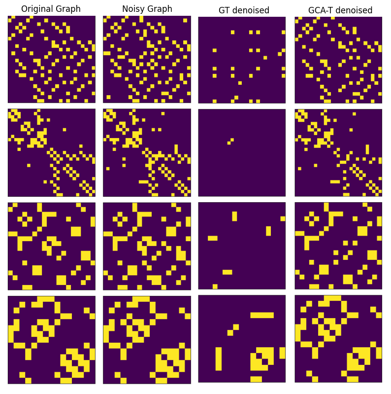
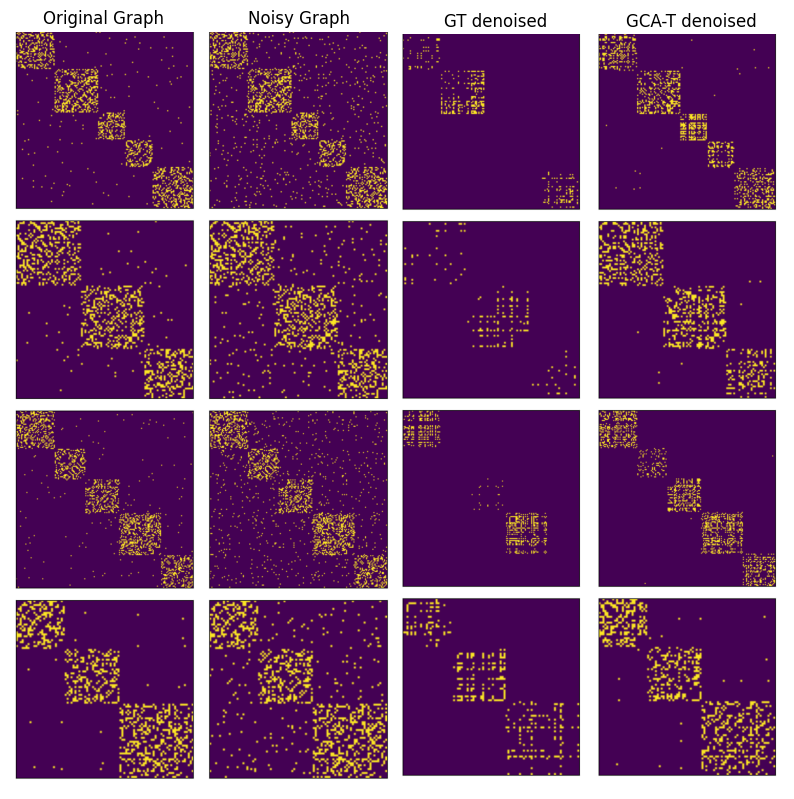
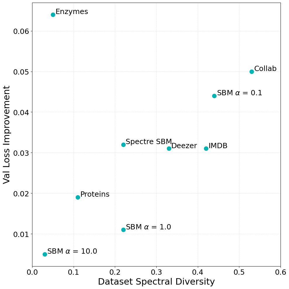
Figure 1: Quantitative and Qualitative Denoising comparison of GT and GCAT.. a — ENZYMES dataset, b — SPECTRE dataset, c — Diversity vs Improvement
As we observe in Figure 1 (c), GCAT has improved denoising performance compared to the GT baseline consistently across all the datasets, as evidenced by the lower validation loss. Figures 1 (a) and 1 (b) show the corresponding qualitative comparison on ENZYMES and SPECTRE, where GCAT’s reconstructions more faithfully recover the structure of the original graph than GT’s. Furthermore, Figure 1 (c) shows that the margin of improvement for each dataset is strongly correlated with the estimated spectral diversity of the dataset, which is in line with our expectation from Theorem 1. This validates the idea that our proposed spectral diversity metric is indeed a strong predictor of the improvement gained by utilizing spectral information directly in the attention mechanism. We approximate the spectral diversity using a KNN approach detailed in Appendix 7.5 to estimate \(\mathbb{E}[B \mid \widetilde{\Lambda}_k]\).
4.4 Generative Experiments↩︎
We evaluate the GCAT architecture in two generative settings. (1) Our main setting mirrors the denoising experiments and our theoretical results: we use the same diffusion training and inference pipeline as DiGress [8], but with the GT or GCAT architecture as the denoiser. (2) We additionally integrate GCAT into the full DiGress recipe, keeping all architecture, hyperparameters, and implementation details as in the published code base — except training steps, which we cap at 88k for SPECTRE-SBM and 300k for ENZYMES (from the published 550k) due to computational and time constraints. MMDs are evaluated every \(4{,}400\) optimiser steps for SPECTRE-SBM, matching upstream’s \(100\)-epoch \(\times\) sample-every-\(4\) cadence, and every \(75{,}000\) for ENZYMES.
| Dataset | Recon LogP \(\uparrow\) | NLL \(\downarrow\) | Spec MMD \(\downarrow\) | Clust MMD \(\downarrow\) | Deg MMD \(\downarrow\) | Orbit MMD \(\downarrow\) |
|---|---|---|---|---|---|---|
| SBM (\(\alpha=0.1\)) | -101.76 | 532.35 | 0.0346 | 0.0233 | 0.0496 | 0.0433 |
| -30.37 | 505.94 | 0.0214 | 0.0257 | 0.0268 | 0.0416 | |
| SBM (\(\alpha=1.0\)) | -112.70 | 576.67 | 0.0721 | 0.0157 | 0.0954 | 0.0240 |
| -31.66 | 544.44 | 0.0247 | 0.0163 | 0.0135 | 0.0220 | |
| SBM (\(\alpha=10\)) | -70.31 | 565.66 | 0.0562 | 0.0166 | 0.0047 | 0.1233 |
| -30.88 | 548.21 | 0.0186 | 0.0156 | 0.0025 | 0.0495 | |
| SPECTRE | -1925.37 | 5044.54 | 0.0172 | 0.0743 | 0.0151 | 0.1405 |
| -1024.65 | 4885.99 | 0.0801 | 0.0718 | 0.0075 | 0.1553 | |
| ENZYMES | -182.88 | 530.31 | 0.0502 | 0.0478 | 0.0956 | 0.0541 |
| -28.26 | 424.79 | 0.0458 | 0.0431 | 0.0458 | 0.2692 | |
| PROTEINS | -354.86 | 968.25 | 0.0885 | 0.0993 | 0.1949 | 0.0616 |
| -122.28 | 838.50 | 0.0310 | 0.0514 | 0.0257 | 0.0331 | |
| IMDB | -55.13 | 275.21 | 0.1249 | 0.3591 | 0.1405 | 0.3800 |
| -13.39 | 208.99 | 0.0278 | 0.2608 | 0.0319 | 0.4133 | |
| COLLAB | -1489.94 | 3588.22 | 0.1465 | 0.0270 | 0.1337 | 0.2144 |
| -1189.15 | 3136.62 | 0.3429 | 0.3399 | 0.3593 | 0.9954 | |
| DEEZER | -177.88 | 502.30 | 0.0147 | 0.0226 | 0.0235 | 0.3136 |
| -49.26 | 414.70 | 0.0289 | 0.0568 | 0.0370 | 0.5548 |
4pt
GCAT vs GT Results. As the results in Table 1 show, the gains in denoising loss translate to uniform improvement in logP and NLL across datasets, when using GCAT in generative diffusion. With the exception of COLLAB and DEEZER, these improved training metrics typically also translate to improved structural metrics in the generated samples. This improvement can also qualitatively be seen in generated graphs when compared to reference graphs from the datasets in Figure 2.
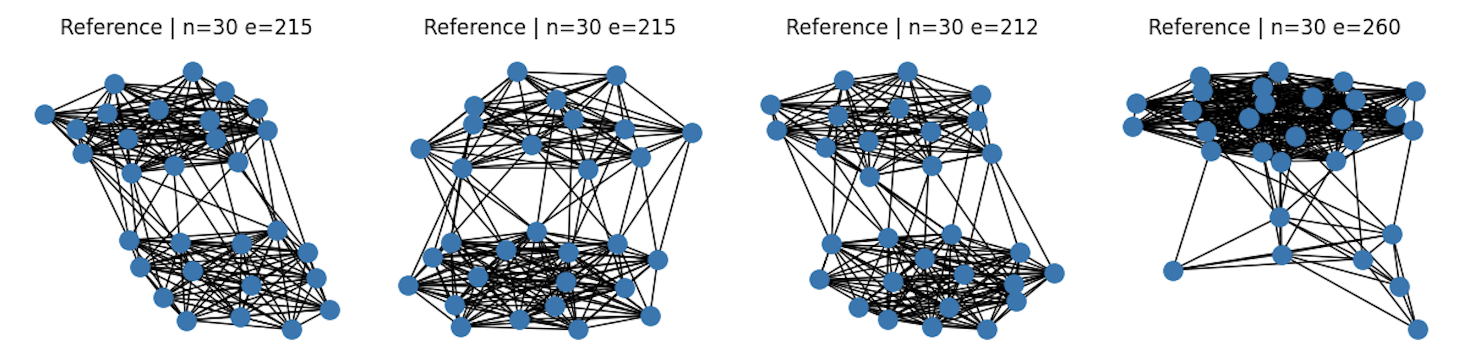
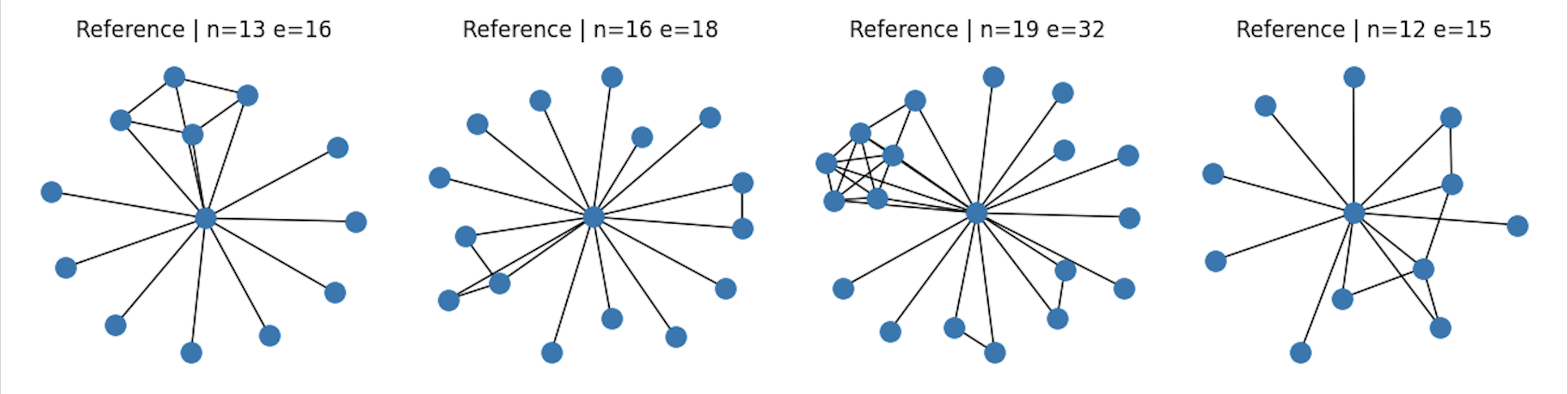
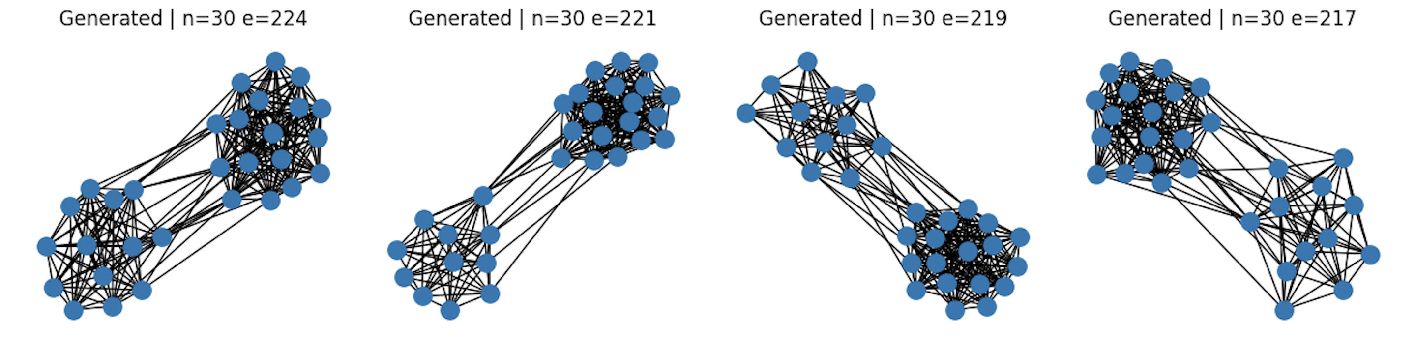
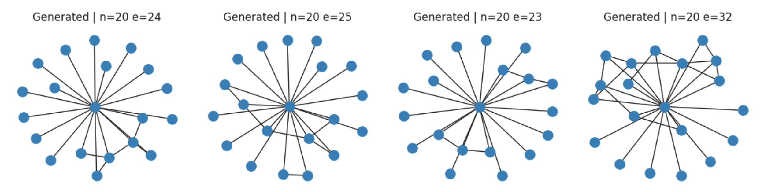
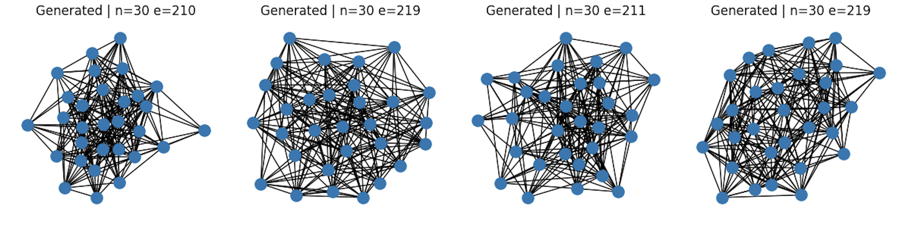
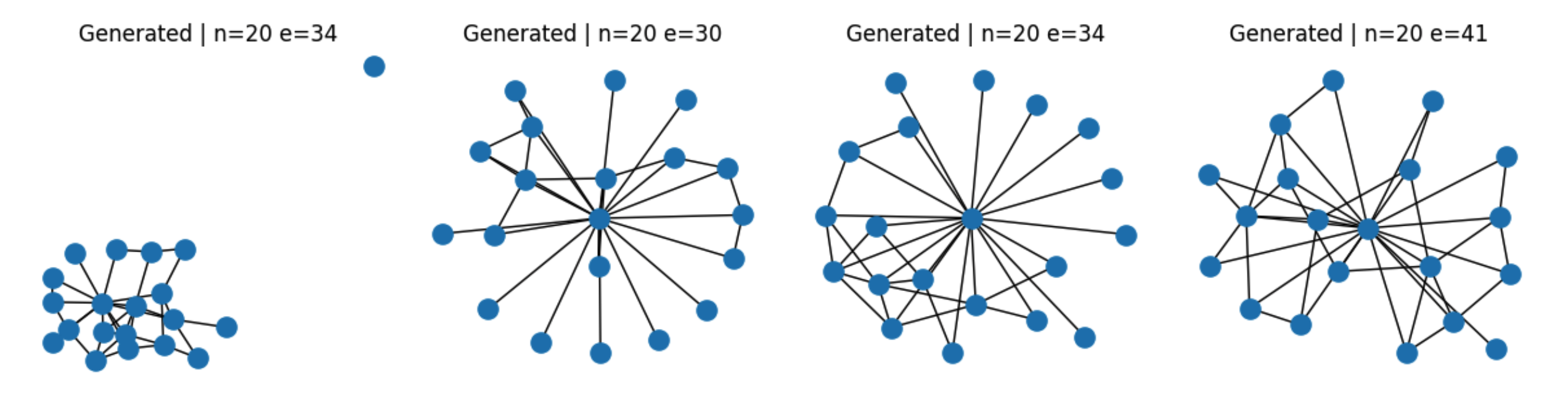
Figure 2: Top: Reference graphs sampled from the dataset, Middle: Graphs generated using with GCAT, Bottom: Graphs generated using GT, Left: two-community SBM graphs, and Right: and ego-network graphs..
DiGress Results. We evaluate on SPECTRE-SBM [30] and ENZYMES [31], two standard literature benchmarks. On SPECTRE-SBM we follow the protocol of DiGress [8]: the fixture contains 200 graphs of up to 200 nodes drawn from a 2–5-community stochastic block model. On ENZYMES we follow HiGen [34]. Following HiGen, we report raw \(\mathrm{MMD}^2\) on the degree, clustering-coefficient, orbit-count, and normalised-Laplacian-spectrum distributions. Each evaluation samples 40 graphs on both datasets.
We observe that the variants leveraging spectral and graph convolutional attention roughly achieve parity with vanilla DiGress in generation quality as measured by MMDs, including when using R-PEARL instead of the eigen-decomposition based features. This gives some evidence that it is indeed sufficient to incorporate the spectral information via GCA + R-PEARL, and expensive eigen-decomposition is not required. Full numbers and qualitative samples are in Appendix 7.1; per-metric training trajectories in Table 8, Appendix 7.4.
Crucially, we see in Table 2 that this parity comes with a noticeable speedup in inference (up to \(19\%\) for the PEARL + GCA variant on SBM) from eliminating the node feature computation and eigendecomposition cost. Because wall-clock time here is dominated by whether an eigendecomposition is computed per step, the payoff scales with graph size: on the larger SBM graphs (\(n_{\max}{=}200\)) all R-PEARL variants are faster, whereas on the small ENZYMES graphs (\(n_{\max}{=}126\)) the fixed overhead of the random-feature GNN can swamp the saving (e.g. PEARL is \(+14\%\)). This suggests that as graph size grows, using our variant with R-PEARL and Graph Convolutional attention could potentially lead to even larger gains in inference time without sacrificing generation quality.
| Dataset | Variant | Params | Inference vs base |
|---|---|---|---|
| SBM (\(n_{\max}{=}200\)) | DiGress (eigh) | 7.1M | — |
| PEARL | 7.2M | -6% | |
| PEARL + GCA | 11.9M | -19% | |
| DiGress (eigh) | 7.1M | — | |
| PEARL | 7.2M | +14% | |
| PEARL + GCA | 11.9M | -14% |
5 Conclusions↩︎
We studied graph denoising from a spectral perspective and used this view to clarify why attention-based architectures such as DiGress can perform well in graph denoising and diffusion. Our analysis shows that standard linear attention is fundamentally limited under a denoising objective, since it can only learn an average spectral denoising rule over the training distribution, which becomes suboptimal when graphs exhibit heterogeneous spectra. In contrast, for graph distributions with community-like spectra and sufficiently high spectral diversity, attention mechanisms that adapt to the noisy input spectrum can implement an optimal shrinkage-like estimator, thereby provably improving over estimators that are agnostic to the observed spectrum. We formalized this ideal through Spectral Attention, identified spectral diversity as the quantity governing its advantage, and proposed Graph Convolutional Attention (GCA) as a practical permutation-equivariant realization based on graph-filtered query and key projections. In the SBM regime, we showed that GCA asymptotically matches the ideal spectral mechanism, while the softmax nonlinearity can provide additional denoising by approximately projecting noisy eigenvectors onto the clean eigenspace. Empirically, the theory is reflected in practice: replacing standard attention with GCA consistently improves graph denoising across synthetic and real datasets, and the gains scale with spectral diversity. The same phenomenon transfers to diffusion models, where preserving this shrinkage-style capacity makes it possible to remove costly spectral node features while remaining competitive, as in the DiGress ablations, and to improve performance on suitable datasets by explicitly incorporating this inductive bias. Overall, our results suggest that spectral adaptation is a key ingredient for effective graph denoising and generative diffusion, and provide both a theoretical explanation and a practical architectural principle for designing stronger graph diffusion models.
Supplementary Materials for
“Understanding Graph Denoising”
6 Limitations and Future Directions↩︎
Expanding the scope of the experiments to more graph benchmark datasets, both real and synthetic could potentially help further validate the merit of GCA and illuminate its potential failure modes.
Furthermore, the exact role of R-PEARL (and in general other types of positional encodings that could be used instead of eigenvectors) can be explored further both theoretically and in practice. Studying the interaction between R-PEARL embeddings and the GCA architecture is a promising direction. On the theoretical side, parts of our analysis are limited to Stochastic Block Models. Considering families of graphs in future work could further strengthen the theoretical message ad our understanding of graph denoising and diffusion.
Finally, our empirical comparisons on SOTA graph diffusion is limited in number of training seeds, dataset variety and hyperparameter ablations. More computational resources and time is required to make these results more statistically meaningful and the results should therefore be seen as exploratory evidence, and cannot support definitive conclusions.
7 Experimental Details and Additional Results↩︎
7.1 DiGress generative ablation results↩︎
The headline numbers and generated samples for the DiGress ablation panel referenced in Section 4 are reproduced below. Table 3 reports the best per-metric value per variant within the per-panel-minimum step horizon (88k for SPECTRE-SBM, 300k for ENZYMES); Figure 3 shows reference graphs alongside generated samples from the upstream DiGress baseline and the R-PEARL + GCAT variant. Hyperparameters, optimisation, and evaluation cadence shared across these runs are documented in Appendix 7.3.4.
| Dataset | Variant | Spec MMD\(^2\) \(\downarrow\) | Clust MMD\(^2\) \(\downarrow\) | Deg MMD\(^2\) \(\downarrow\) | Orbit MMD\(^2\) \(\downarrow\) | SBM acc.\(\uparrow\) |
|---|---|---|---|---|---|---|
| SPECTRE-SBM | DiGress (baseline) | 0.2102 | 0.1306 | 0.1803 | 0.0909 | 0.5625 |
| DiGress + R-PEARL | 0.2102 | 0.1297 | 0.1813 | 0.0991 | 0.5312 | |
| DiGress + R-PEARL + Spec.Attn. | 0.2088 | 0.1303 | 0.2001 | 0.0948 | 0.4062 | |
| DiGress + R-PEARL + GCAT | 0.2081 | 0.1292 | 0.1833 | 0.0962 | 0.2500 | |
| ENZYMES | DiGress (baseline) | 0.1960 | 0.1042 | 0.1803 | 0.1056 | — |
| DiGress + R-PEARL | 0.1881 | 0.0967 | 0.1814 | 0.0971 | — | |
| DiGress + R-PEARL + Spec.Attn. | 0.1876 | 0.0974 | 0.1852 | 0.1332 | — | |
| DiGress + R-PEARL + GCAT | 0.1993 | 0.0981 | 0.1924 | 0.2384 | — |
4pt
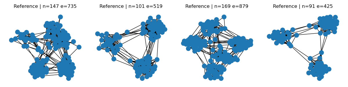
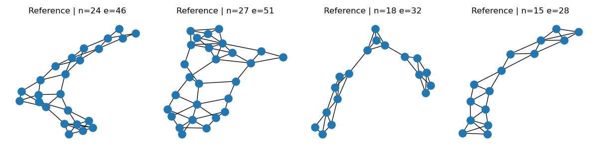
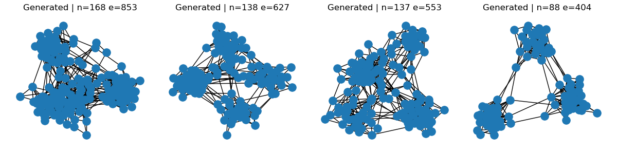
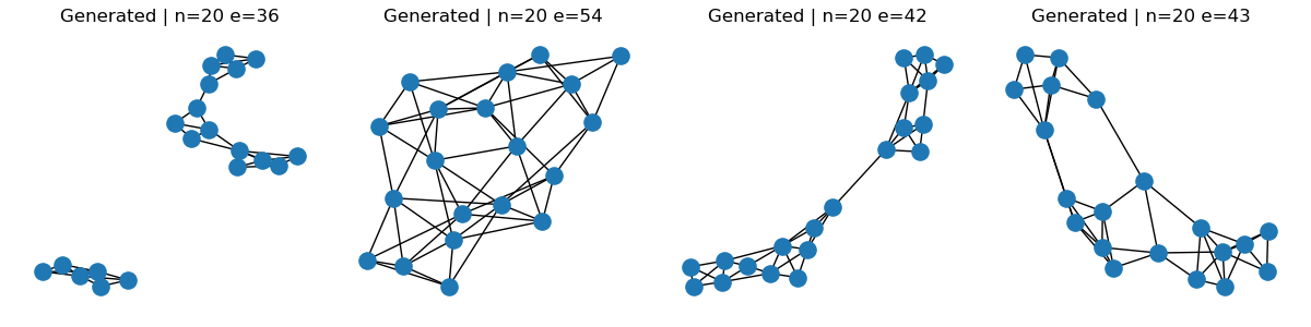
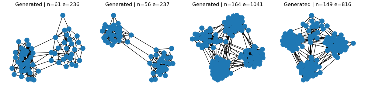
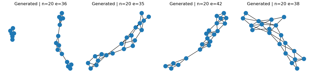
Figure 3: Top: Reference graphs from the dataset, Middle: Generated with the DiGress + R-PEARL + GCAT variant. Bottom: Generated with DiGress baseline..
7.2 Datasets↩︎
We evaluate on a mix of real benchmark graphs drawn from PyTorch Geometric’s TUDataset collection, the SPECTRE stochastic block model (SBM) benchmark [30], and synthetic SBMs sampled with controllable block-size heterogeneity. All graphs are treated as undirected and unattributed: we
keep only the adjacency structure and discard any node or edge labels supplied by the source dataset. Unless stated otherwise, we use a \(70/10/20\) train/validation/test split with a fixed seed.
7.2.1 Real datasets↩︎
We use five collections of variable-size unattributed graphs.
PROTEINS [31], from TUDataset: \(1\,113\) protein-structure graphs in which nodes are secondary-structure elements connected when they are neighbours in the amino-acid sequence or in 3D space. Graph size ranges up to \(620\) nodes, with most graphs in the few-tens to low-hundreds range.
ENZYMES [31], from TUDataset: \(600\) enzyme tertiary-structure graphs spanning the six EC top-level classes. Graph size ranges up to \(126\) nodes, typically \(\approx 30\)–\(60\) nodes per graph.
IMDB-BINARY [32], from TUDataset: \(1\,000\) movie-collaboration ego networks in which nodes are actors/actresses and edges connect those that appeared together in a film. Graph size ranges up to \(136\) nodes with a strongly skewed distribution toward smaller, dense ego networks.
COLLAB [32], from TUDataset: \(5\,000\) scientific-collaboration ego networks built from three physics communities. Graph size ranges up to \(492\) nodes, with heavy-tailed size and degree distributions.
DEEZER-EGO-NETS [33]: \(9\,629\) ego networks of Deezer users, with edges representing mutual-friend relationships in the ego’s neighbourhood. Graph size ranges up to \(363\) nodes; the distribution is dominated by ego networks of a few dozen nodes.
In all five cases we drop the original node and edge attributes and predict the binary adjacency only. This matches the unconditional graph-generation setting used in prior work [8], [35], [36]. Splits use the PyG-default ordering with a fixed seed of \(42\) and a \(70/10/20\) train/val/test ratio.
7.2.2 SPECTRE SBM benchmark↩︎
We additionally use the SBM benchmark released with the SPECTRE evaluation suite [30] and adopted as the canonical SBM
evaluation setting by DiGress [8]. The fixture contains \(200\) SBM graphs generated with \(2\)–\(5\) communities of variable size, intra-block edge probability \(p_{\mathrm{intra}}\approx 0.30\), and inter-block edge probability \(p_{\mathrm{inter}}\approx 0.005\); node counts range over \(44 \leq n \leq 187\). We use the upstream \(128/32/40\) train/val/test split
(torch.randperm(200) with seed \(0\)) so that our results are byte-comparable with published DiGress numbers. Quantitative evaluation reports the SPECTRE-style maximum mean discrepancy (MMD) over degree,
clustering, and orbit-count distributions, plus the SBM-likelihood Wald-test accuracy whose null distribution uses the same \((p_{\mathrm{intra}},p_{\mathrm{inter}})\) parameters.
7.2.3 Synthetic SBMs with controllable block-size heterogeneity↩︎
To probe how each method handles community structure under controlled conditions, we generate synthetic SBM datasets at two graph sizes, \(n=100\) and \(n=200\) (presets
sbm_n100, sbm_n200). Block counts are sampled uniformly from \(K\in\{2,3,4\}\), with maximum block sizes of \(50\) and \(60\)
respectively. Edge probabilities default to \(p_{\mathrm{intra}}=1.0\) and \(p_{\mathrm{inter}}=0.0\) (i.e. disjoint cliques), but can be varied along ranges to expose the model to a
spectrum of community contrast.
The key controlled axis is block-size heterogeneity, governed by a Dirichlet concentration parameter \(\alpha\) (in code: graph_config.block_size_alpha). For each synthetic graph we sample a
block-size partition \[(s_1, \ldots, s_K) \;\sim\; n \cdot \mathrm{Dirichlet}(\alpha, \ldots, \alpha), \label{eq:dirichlet-blocks}\tag{7}\] rounded to integers summing
to \(n\), with a minimum block size of one. The concentration \(\alpha\) smoothly interpolates between two regimes: small \(\alpha\) (e.g.\(\alpha\to 0^{+}\)) concentrates mass on a single block and produces strongly unbalanced communities, while large \(\alpha\) (e.g.\(\alpha\gg 1\))
flattens the simplex and recovers near-equal-sized blocks (the limit \(\alpha\to\infty\) matches the equal-partition baseline). This single knob lets us study how generative models behave under increasing
block-size imbalance while holding \(n\), \(K\), and \((p_{\mathrm{intra}},p_{\mathrm{inter}})\) fixed. We sweep \(\alpha\)
over a logarithmic grid in the experiments of Section 4. Block sizes are re-sampled per graph; intra- and inter-block edges are then drawn independently from \(\mathrm{Bernoulli}(p_{\mathrm{intra}})\) and \(\mathrm{Bernoulli}(p_{\mathrm{inter}})\) as in the standard SBM definition.
7.3 Architectural details↩︎
7.3.1 Graph Transformer and Graph Convolutional Attention Transformer↩︎
7.3.1.1 Shared pipeline.
We extract the top-\(k\) eigenvectors \(V \in \mathbb{R}^{n \times k}\) of \(A\) and lift them to the model dimension \(d\): \[X^{(0)} = V\, W_{\mathrm{in}}, \qquad W_{\mathrm{in}} \in \mathbb{R}^{k \times d}.\] Each of the first \(L-1\) blocks applies a residual multi-head attention update with \(h\) heads of dimension \(d_k = d_v = d/h\): \[X^{(\ell+1)} = \mathrm{LN}\!\left( X^{(\ell)} + \mathrm{MHA}^{(\ell)}\!\big(A,\,X^{(\ell)}\big) \right), \qquad \ell = 0,\dots,L-2,\] where, given queries, keys, and values \(Q^{(\ell)}, K^{(\ell)}, V^{(\ell)}\), each head computes \[S_i^{(\ell)} = \frac{Q_i^{(\ell)} {K_i^{(\ell)}}^{\!\top}}{\sqrt{d_k}}, \qquad \mathrm{Attn}_i^{(\ell)} = \mathrm{softmax}\!\big(S_i^{(\ell)}\big)\,V_i^{(\ell)}, \qquad i = 1,\dots,h,\] The final block produces no node features; its per-head scores \(S^{(L-1)} \in \mathbb{R}^{h \times n \times n}\) are mixed into the edge logits by a learned linear combination, \[\widehat{A} = \sum_{i=1}^{h} w_i\, S_i^{(L-1)} + b, \qquad w \in \mathbb{R}^{h}.\]
The two models differ only in the \(Q\)/\(K\) projections inside each block.
Graph Transformer \[Q^{(\ell)} = X^{(\ell)} W_Q^{(\ell)}, \qquad K^{(\ell)} = X^{(\ell)} W_K^{(\ell)}.\]
Graph Convolutional Transformer \[Q^{(\ell)} = \mathrm{LN}\!\left( \sum_{p=0}^{P-1} A^{\,p}\, X^{(\ell)}\, W_{Q,p}^{(\ell)} \right), \qquad K^{(\ell)} = \mathrm{LN}\!\left( \sum_{p=0}^{P-1} A^{\,p}\, X^{(\ell)}\, W_{K,p}^{(\ell)} \right).\] The queries and keys become learnable polynomials of the noisy adjacency, allowing two nodes to attend on the basis of their \(P\)-hop neighborhoods in \(A\).
7.3.2 Generative Experiments with GT and GCAT Denoisers↩︎
The setup is similar to the one described in 7.3.4. The hyperparameters specific to these runs are provided in Table 4.
7.3.3 R-PEARL↩︎
The encoder samples \(s = 32\) standard Gaussian features per node, propagates them through three message-passing layers over the symmetrically normalised adjacency \(D^{-1/2} \widetilde{A} D^{-1/2}\), and projects the result to a \(d_{\text{PEARL}} = 16\)-dimensional per-node embedding. Each message-passing layer applies a two-layer MLP with ReLU activation, hidden width \(64\), and LayerNorm, adding a residual connection where input and output widths match. The resulting embedding is concatenated to per-node cycle counts at lengths \(3, 4, 5\) to form the per-node features; per graph we keep the normalised graph size \(n_{\mathrm{valid}} / n_{\max}\) and cycle counts at lengths \(3, 4, 5, 6\). Total widths \(\Delta(d_X, d_E, d_y) = (3 + d_{\text{PEARL}}, 0, 5)\), compared with \((6, 0, 11)\) for DiGress’s eigendecomposition path. To make evaluation deterministic, we fix the eval-time features to a single seeded Gaussian draw of shape \((1, n_{\max}, s)\), shared across each evaluation batch. Training continues to draw fresh features per forward pass, so the model sees the full R-PEARL feature distribution during optimisation; at evaluation we therefore report one specific R-PEARL realisation rather than a Monte Carlo average over draws.
7.3.4 DiGress and variants↩︎
Our generative DiGress runs reproduce the upstream SPECTRE-SBM recipe of DiGress [8] and cross-validate against the publicly available SBM checkpoint shipped with GDPO [38], which was retrained from the upstream recipe verbatim and provides an independent set of weights for sanity checks.
7.3.4.1 Architecture.
The denoiser is the upstream DiGress XEy graph transformer: a stack of \(L = 8\) blocks that jointly update node features \(X\), edge features \(E\), and a global vector \(y\), with FiLM-style cross-modulation between the three streams. Hidden widths are \(d_X = 256\), \(d_E = 64\), \(d_y = 64\) with \(8\) attention heads, point-wise feed-forward widths \((d_{\mathrm{ff}X}, d_{\mathrm{ff}E}, d_{\mathrm{ff}y}) = (256, 64, 2048)\) for SPECTRE-SBM and \((256, 64, 256)\) for ENZYMES, input/output MLP widths \((128, 64, 128)\), and a learned timestep channel concatenated to \(y\). We use the \(K = 1\) abstract-node convention (one node class, two edge classes) for both datasets. The SPECTRE-SBM choice \(d_{\mathrm{ff}y} = 2048\) matches the actual shape of the GDPO SBM checkpoint, which was trained at this width despite the value \(256\) recorded in Vignac’s published config; we adopt the checkpoint’s shape so the released weights remain loadable into our model. ENZYMES, where no comparable checkpoint is released, uses Vignac’s \(d_{\mathrm{ff}y} = 256\).
7.3.4.2 Structural augmentation.
For the vanilla DiGress runs we follow upstream DiGress in augmenting the inputs with hand-crafted structural features. Per node, we concatenate cycle counts at lengths \(3, 4, 5\) (scaled by \(1/10\) and clipped at \(1\)), an indicator that the node does not lie in the largest connected component, and the two lowest non-trivial eigenvectors of the noisy graph Laplacian evaluated at the node. Per graph, we add the normalised graph size \(n_{\mathrm{valid}} / n_{\max}\), cycle counts at lengths \(3, 4, 5, 6\) (also scaled and clipped), the number of connected components, and the five lowest non-trivial Laplacian eigenvalues. Total feature widths \(\Delta(d_X, d_E, d_y) = (6, 0, 11)\). Cycle counts are computed from powers of the binary noisy adjacency; the spectral channels require an eigendecomposition of the noisy Laplacian at every diffusion step. The R-PEARL alternative described in Section 7.3.3 drops the spectral channels and replaces them with the R-PEARL embedding.
7.3.4.3 Diffusion process.
A categorical forward process with the IDDPM cosine schedule [37] on \(T = 1000\) steps and an empirical-marginal limit distribution measured from the training loader at setup. We use the unmodified IDDPM cosine schedule (DiGress’s edge-class-dependent variant for molecular datasets is not used here, since SBM and ENZYMES are binary-edge graphs). The reverse process predicts class probabilities at each step; sampling is ancestral.
7.3.4.4 Optimisation.
AdamW with learning rate \(2 \times 10^{-4}\), weight decay \(10^{-12}\), AMSGrad enabled, no learning-rate scheduler, no gradient clipping, and no EMA. The training loss is categorical cross-entropy with edge weight \(\lambda_E = 5\) on top of the standard variational lower bound. Seed \(666\) matches the GDPO retrain so the run lands in a basin comparable to the released checkpoint; Vignac’s repository defaults to seed \(0\). Batch size is \(12\), and the published \(128/32/40\) train/validation/test split of the 200-graph SPECTRE fixture matches the upstream byte-for-byte.
7.3.4.5 Schedule.
\(5.5 \times 10^{5}\) optimiser steps. Upstream specifies \(50{,}000\) epochs at batch size \(12\) on \(128\) training graphs, equivalent to \(\approx 5.5 \times 10^{5}\) steps; we adopt the step-based form. Reported runs reach \(\approx 88\)k steps for SPECTRE-SBM and \(\approx 300\)k for ENZYMES under our compute budget (Section 4). Validation and full sampling/MMD evaluation share a step-based gate: every \(4{,}400\) steps for SPECTRE-SBM (matching upstream Vignac’s \(100\)-epoch validation \(\times\) sample-every-\(4\) cadence) and every \(75{,}000\) steps for ENZYMES (panel-calibrated for evaluation cost). Each evaluation samples \(40\) graphs at clustering kernel \(\sigma = 0.1\).
7.3.4.6 Variants.
We sweep two architectural axes: the input-augmentation choice (DiGress’s structural augmentation above or the R-PEARL embeddings of Section 7.3.3) and the attention-projection choice. The first attention-side replacement substitutes \(Q/K/V\) with polynomial spectral filters in the noisy Laplacian eigenvalues using \(k_{\text{spec}} = 16\) eigenpairs and three polynomial taps. The second replaces \(Q/K/V\) with three-tap polynomials in the adjacency itself, run in two normalisations: the symmetrically normalised adjacency \(D^{-1/2} A D^{-1/2}\) and the raw adjacency \(A\). Of the six combinations on this \(2 \times 4\) grid (two augmentations \(\times\) four projection choices), five are evaluated; the cross of DiGress’s structural augmentation with the graph-convolution attention is not currently run.
| Attention-projection ablations | ||
|---|---|---|
| Variant | \(Q\)/\(K\)/\(V\) projection | Polynomial taps |
| Linear attention | linear | — |
| Spectral attention | polynomial in \(\tilde \Lambda\) (\(k_{\text{spec}} = 16\) eigenpairs of \(\tilde A\)) | \(3\) |
| Graph-conv attention (normalised) | polynomial in \(D^{-1/2} A D^{-1/2}\) | \(3\) |
| Graph-conv attention (raw) | polynomial in \(A\) | \(3\) |
| Dataset-specific overrides | ||
| Setting | SPECTRE-SBM | ENZYMES |
| \(d_{\mathrm{ff}y}\) | \(2048\) (matches GDPO checkpoint) | \(256\) (Vignac default) |
| \(n_{\max}\) | \(200\) | \(126\) |
| Train/val/test split | \(128/32/40\) on the published \(200\)-graph fixture | \(70/10/20\) percentage split with fixed seed |
7.3.4.7 Per-step wall-clock.
Table 7 reports the mean per-step optimiser wall-clock time logged by each post-fix run. The relative cost depends strongly on graph size: on the \(n=200\) SPECTRE-SBM fixture the \(O(n^3)\) Laplacian eigendecomposition that DiGress’s structural augmentation performs at every diffusion step dominates, and replacing it with R-PEARL gives a \(\sim\)5% per-step speedup; on ENZYMES, where graphs typically have \(\le 60\) nodes, the eigendecomposition is cheap, the R-PEARL message-passing fixed cost is not amortised, and every R-PEARL variant is slower per step than the DiGress baseline.
| Dataset | Variant | \(n_{\text{steps}}\) | Mean (s) | Median (s) | Speedup vs vignac |
|---|---|---|---|---|---|
| SPECTRE-SBM | DiGress (baseline) | 2254 | 0.5184 | 0.5127 | — |
| DiGress + R-PEARL | 2372 | 0.4937 | 0.4857 | +4.8% | |
| DiGress + R-PEARL + Spec.Attn. | 2200 | 0.5345 | 0.5277 | -3.1% | |
| DiGress + R-PEARL + GCAT | 2390 | 0.4933 | 0.4875 | +4.8% | |
| ENZYMES | DiGress (baseline) | 9977 | 0.1218 | 0.1068 | — |
| DiGress + R-PEARL | 7404 | 0.1647 | 0.1498 | -35.2% | |
| DiGress + R-PEARL + Spec.Attn. | 6207 | 0.1962 | 0.1813 | -61.1% | |
| DiGress + R-PEARL + GCAT | 8768 | 0.1391 | 0.1277 | -14.2% |
4pt
7.4 Additional DiGress results↩︎
Table 3 in the main body reports the per-metric best across validation cycles up to the per-panel minimum step (88k for SPECTRE-SBM, 300k for ENZYMES) so longer-running variants do not gain extra “best” attempts. Table 8 below removes that cap and instead annotates each best with the optimiser step at which it occurred (as a superscript), so the trajectory of each metric across training is visible at a glance.
| Dataset | Variant | Spec MMD\(^2\) \(\downarrow\) | Clust MMD\(^2\) \(\downarrow\) | Deg MMD\(^2\) \(\downarrow\) | Orbit MMD\(^2\) \(\downarrow\) | SBM acc.\(\uparrow\) |
|---|---|---|---|---|---|---|
| SPECTRE-SBM | DiGress (baseline) | 0.2102\(^{(22k)}\) | 0.1292\(^{(110k)}\) | 0.1803\(^{(88k)}\) | 0.0909\(^{(22k)}\) | 0.6250\(^{(110k)}\) |
| DiGress + R-PEARL | 0.2102\(^{(44k)}\) | 0.1297\(^{(66k)}\) | 0.1813\(^{(22k)}\) | 0.0991\(^{(88k)}\) | 0.5312\(^{(88k)}\) | |
| DiGress + R-PEARL + Spec.Attn. | 0.2088\(^{(88k)}\) | 0.1303\(^{(44k)}\) | 0.2001\(^{(44k)}\) | 0.0948\(^{(88k)}\) | 0.4062\(^{(44k)}\) | |
| DiGress + R-PEARL + GCAT | 0.2081\(^{(44k)}\) | 0.1292\(^{(88k)}\) | 0.1833\(^{(44k)}\) | 0.0962\(^{(66k)}\) | 0.3750\(^{(110k)}\) | |
| ENZYMES | DiGress (baseline) | 0.1960\(^{(150k)}\) | 0.0961\(^{(375k)}\) | 0.1803\(^{(150k)}\) | 0.1037\(^{(375k)}\) | — |
| DiGress + R-PEARL | 0.1881\(^{(150k)}\) | 0.0967\(^{(75k)}\) | 0.1814\(^{(225k)}\) | 0.0971\(^{(300k)}\) | — | |
| DiGress + R-PEARL + Spec.Attn. | 0.1876\(^{(225k)}\) | 0.0974\(^{(75k)}\) | 0.1852\(^{(225k)}\) | 0.1332\(^{(150k)}\) | — | |
| DiGress + R-PEARL + GCAT | 0.1993\(^{(225k)}\) | 0.0981\(^{(75k)}\) | 0.1818\(^{(375k)}\) | 0.1171\(^{(375k)}\) | — |
4pt
On SPECTRE-SBM, MMDs and the SBM-accuracy Wald test peak at different points along training. Most MMD bests sit in the first \(\approx 22\)–\(88\)k optimiser steps; the SBM accuracy of three of the four variants only peaks at \(88\)–\(110\)k. The R-PEARL + GCAT variant illustrates the asymmetry: best spectral MMD by step \(44\)k but best SBM accuracy at step \(110\)k. The pattern is suggestive rather than universal – the vanilla DiGress run reaches its best clustering MMD only at \(110\)k, and pearl + spectral attention peaks SBM accuracy at \(44\)k. We read the table as evidence that MMD-style sample quality and Wald-test community structure are not perfectly co-monotone in training, and leave a more careful longitudinal analysis to future work.
7.5 Spectral diversity metric↩︎
We estimate the improvement-gap surrogate of Theorem 1 non-parametrically and report it on a normalised scale that supports cross-dataset comparison. The estimand, the plug-in estimator that approximates it from a finite sample, the frame-alignment step that makes the cross-graph average meaningful, the bias floor introduced by the plug-in, and the permutation-null calibration that removes it are detailed below.
7.5.0.1 Population estimand.
For each graph \(i\) in a dataset, let \(A_i\) be its clean adjacency, \(\widetilde{A}_i = A_i + \mathcal{E}_i\) a noisy observation, and \((\widehat V_{k,i}, \widetilde{\Lambda}_{k,i})\) the noisy top-\(k\) eigenpair of \(\widetilde{A}_i\). Define \(B_i = \widehat V_{k,i}^\top A_i \widehat V_{k,i}\), the clean adjacency expressed in the noisy top-\(k\) eigenbasis. Theorem 1 identifies the gap between linear- and spectral-attention losses with \(g = \mathbb{E}\|\mathbb{E}[B \mid \widetilde{\Lambda}_k] - \mathbb{E}[B]\|_F^2\), the variance of the optimal spectral predictor \(f^\star(\widetilde{\Lambda}_k) = \mathbb{E}[B \mid \widetilde{\Lambda}_k]\). Dividing by the total variance \(\mathrm{tr}(\mathrm{Cov}\, B) = \mathbb{E}\|B - \mathbb{E}[B]\|_F^2\) yields the fraction of variance explained, \[\mathrm{FVE} \;=\; \frac{g}{\mathrm{tr}(\mathrm{Cov}\, B)} \;\in\; [0, 1],\] which by the law of total variance equals the \(R^2\) of \(f^\star\) when used to predict \(B\) from \(\widetilde{\Lambda}_k\) — equivalently, the relative loss improvement of optimal spectral attention over optimal linear attention (Propositions 1–2).
7.5.0.2 Plug-in estimator.
The population quantities \(f^\star\), \(g\), and \(\mathrm{tr}(\mathrm{Cov}\, B)\) are inaccessible; we replace each by a finite-sample plug-in. Given \(N\) graphs with paired observations \(\{(B_i, \widetilde{\Lambda}_{k,i})\}_{i=1}^{N}\), we estimate the optimal predictor by kNN regression on the noisy eigenvalues, \[\widehat B_i \;=\; \frac{1}{m} \sum_{j \in \mathcal{N}_m(i)} B_j,\] where \(\mathcal{N}_m(i)\) is the set of \(m\) graphs other than \(i\) whose eigenvalue vectors are closest to \(\widetilde{\Lambda}_{k,i}\) in Euclidean distance. The plug-in estimates of \(g\) and the total variance use the same sample, \[\widehat g \;=\; \frac{1}{N} \sum_{i=1}^{N} \|\widehat B_i - \bar B\|_F^2, \qquad \widehat{\mathrm{tr}(\mathrm{Cov}\, B)} \;=\; \frac{1}{N} \sum_{i=1}^{N} \|B_i - \bar B\|_F^2,\] with \(\bar B = \tfrac{1}{N} \sum_i B_i\). The sample-level statistic is their ratio \[\widehat{\mathrm{FVE}} \;=\; \frac{\widehat g}{\widehat{\mathrm{tr}(\mathrm{Cov}\, B)}}.\] The estimator is non-parametric: no analytic form for \(f^\star\) is assumed.
7.5.0.3 Frame alignment.
The matrix \(B_i\) is not invariant to the gauge of \(\widehat V_{k,i}\): replacing \(\widehat V_{k,i}\) by \(\widehat V_{k,i} Q_i\) for any \(Q_i \in O(k)\) maps \(B_i \to Q_i^\top B_i Q_i\). Averaging matrices across different per-graph frames adds incommensurable quantities and inflates \(\widehat g\), because \(Q_i\) is partly predictable from \(\widetilde{\Lambda}_{k,i}\) (both derive from the same noisy decomposition). We therefore align every \(\widehat V_{k,i}\) via orthogonal Procrustes against a single dataset-wide reference frame, the extrinsic Grassmannian mean of the clean top-\(k\) eigenbases (top-\(k\) left singular vectors of the stacked clean eigenvector blocks). With one common frame, the residual rotation cannot co-vary with \(\widetilde{\Lambda}_k\), and the convention-artefact channel that would otherwise feed a spurious signal into the estimator closes.
7.5.0.4 Bias floor.
Under the null \(B \perp \widetilde{\Lambda}_k\), the neighbours \(\mathcal{N}_m(i)\) are effectively a random subsample of the \(B_j\), so \(\mathrm{Var}(\widehat B_i) \approx \mathrm{Var}(B)/m\) and \(\widehat{\mathrm{FVE}}\) acquires a floor \[\mathbb{E}\bigl[\widehat{\mathrm{FVE}} \;\big|\; B \perp \widetilde{\Lambda}_k\bigr] \;\approx\; \frac{1}{m} - \frac{1}{N-1}.\] For \((m, N) = (10, 200)\) this is approximately \(0.095\). Comparing \(\widehat{\mathrm{FVE}}\) directly to zero is therefore uninformative.
7.5.0.5 Permutation-null calibration.
We estimate the bias floor on each dataset by shuffling the conditioning vectors with a uniformly random permutation \(\pi\) and recomputing the same plug-in ratio, \[\widehat{\mathrm{FVE}}_{\text{null}} \;=\; \widehat{\mathrm{FVE}}\!\bigl(\{(B_i,\, \widetilde{\Lambda}_{k,\pi(i)})\}\bigr).\] The shuffle preserves both marginals and breaks only the joint, so its expectation matches the kNN bias to leading order. The reported quantity is the calibrated margin \(\widehat{\mathrm{FVE}}_{\text{real}} - \widehat{\mathrm{FVE}}_{\text{null}}\), computed per seed before averaging across seeds (paired differencing reduces variance because real and null share the same kNN bias). We require this margin to exceed \(0.10\) and \(\widehat{\mathrm{FVE}}_{\text{null}}\) to remain below \(0.30\); the latter rules out small-\(N\) regimes in which the estimator’s variance grows faster than the signal.
7.5.0.6 Hyperparameters.
We use \(m = 10\) neighbours and sweep \(k \in \{4, 8, 16, 32\}\). The bias-floor formula at \(N \approx 200\) gives \(\widehat{\mathrm{FVE}}_{\text{null}} \approx 0.10\), which is empirically observed across the eight datasets. Noise levels are \(\varepsilon \in \{0.01, 0.05, 0.1, 0.15, 0.2\}\), matching the denoising-experiment grid. Five seeds are used for the paired margin and its standard error. The headline figure reports the Gaussian-noise condition at \(\varepsilon = 0.1\); the DiGress-noise variant produces the same qualitative ordering.
7.5.0.7 Cross-checks.
Two estimator variants run alongside the kNN estimator. A binning estimator partitions graphs into quantile buckets of the spectral gap \(\lambda_1 - \lambda_2\) and computes the classical between-group variance; it agrees with kNN when both are restricted to the 1-D feature, providing an independent estimate of the leading-eigenvalue contribution to the gap. A frame-invariant estimator replaces \(B_i\) with its orthogonal-conjugation invariants \(\bigl(\mathrm{tr}(B_i),\, \|B_i\|_F^2,\, \text{sorted eigvals}(B_i)\bigr)\) and runs through the same kNN pipeline; the Procrustes-aligned and per-graph paths must agree on this target by construction. Both cross-checks track the headline ordering across the eight datasets in the study.
7.5.0.8 Datasets and results.
We compute the calibrated FVE margin on a sweep of four synthetic stochastic block models with controlled diversity and four real graph benchmarks (spectre_sbm, enzymes, proteins, collab). The
synthetic-diversity result shown in Figure 1 (c) is monotone across all \(k\) and replicates under both noise models; on the real benchmarks the calibrated margin exceeds
the calibration threshold on seven of eight datasets, with the failure being the designed null control (the \(\mathrm{diversity}=0\) synthetic SBM).
7.6 Compute resources↩︎
7.6.0.1 Hardware overview.
The denoising experiments of Section 4 (Figure 1) and the denoising-metric runs feeding Figure 1 (c) were trained on a single
workstation with two NVIDIA RTX A5000 GPUs (\(24\) GB GDDR6 VRAM each), \(64\) physical / \(128\) logical CPU cores, and \(\approx
270\) GB host RAM; each run is a single-GPU job. The DiGress generative experiments (Tables 3 and 7) were trained on Modal (modal.com)
using its fast GPU tier, which provisions a single NVIDIA A100 (\(40\) GB HBM2) per container with \(\approx 32\) GB host RAM. The spectral-diversity FVE estimation (Appendix 7.5) is CPU-only and runs on a local workstation; the full sweep (8 datasets \(\times\) 5 seeds \(\times\) 2 frame modes \(\times\) 2 noise types \(\times\) 5 noise levels \(\times\) 4 estimators \(\times\) 4 values of \(k\) \(\times\) real/null) completes in \(\approx 60\) minutes.
7.6.0.2 Wall-clock and total compute (reported runs).
The denoising panel (W&B projects graph-denoising-final-2 and graph-denoising-final-3, \(127\) runs total) ran in median \(\approx 1.6\) minutes and at most
\(\approx 32\) minutes per run, for a cumulative budget of \(\approx 6\) single-GPU-hours on the RTX A5000s. The eight reported DiGress configurations (four variants \(\times\) two datasets) each accumulated \(\approx 17.8\) h of Modal A100 wall-clock at the data freeze, with preempt-resume across the \(24\) h container
timeout, reaching \(\approx 110\)k–\(120\)k optimiser steps on SPECTRE-SBM and \(\approx 310\)k–\(500\)k on ENZYMES (the
ENZYMES graphs are an order of magnitude smaller in node count, so the per-step cost is correspondingly smaller; see Table 7). Cumulatively the eight DiGress runs consume \(\approx
142\) single-A100-hours.
7.6.0.3 Discarded compute.
Initial exploration and iteration until the GDPO baseline was matched amounted to an additional \(\approx 370\) single-A100-hours, with no further details.
8 Proofs↩︎
8.1 Proof of Theorem 2↩︎
Proof. We first show that for a given graph \(A\), \(B := \widetilde{U}^\top A \widetilde{U}\) tends to a deterministic matrix as \(n \to \infty\). We begin by writing \(B\) as:
\[B = \widetilde{U}^\top A \widetilde{U} = \widetilde{U}^\top U \Lambda U^\top \widetilde{U}\]
Consider that \(A\) is low rank therefore we can write: \[A = \sum_{i = 1}^r \lambda_i u_i u_i^\top\]
Thus we have: \[B_{ij} = \sum_{l = 1}^r \lambda_l (\widetilde{u}_i^\top u_l)(\widetilde{u}_j^\top u_l)\]
According to Lemma 3 we have: \[\lim_{n \to \infty} B_{ii} = \lim_{n \to \infty} \sum_{l = 1}^r \lambda_l |\widetilde{u}_i^\top u_l|^2 = \lambda_i \lim_{n \to \infty} |\widetilde{u}_i^\top u_i|^2 + \sum_{l = 1, l \neq i}^r \lambda_l \lim_{n \to \infty} |\widetilde{u}_i^\top u_l|^2\] The sum over \(l \neq i\) tends to zero almost surely, thus we have: \[\lim_{n \to \infty} B_{ii} = \lambda_i \alpha(\lambda_i) = \lambda_i (1 - \frac{\sigma^2}{\lambda_i^2}) = \lambda_i - \frac{\sigma^2}{\lambda_i}\]
for the off-diagonal elements we have: \[\lim_{n \to \infty} B_{ij} = \lim_{n \to \infty} \sum_{l = 1}^r \lambda_l (\widetilde{u}_i^\top u_l)(\widetilde{u}_j^\top u_l) = 0,\] where since \(i \neq j\), one of the inner products will almost surely tend to zero regardless of the value of \(l\).
So, in summary we have for a given fixed graph \(A\), \(B\) tends to a deterministic matrix as \(n \to \infty\): \[\lim_{n \to \infty} B = \alpha(\Lambda)\]
Furthermore, from Lemma 3 we have the deterministic relationship between the noisy and clean eigenvalues: \[\rho(\lambda_i) = \widetilde{\lambda}_i = \lambda_i + \frac{\sigma^2}{\lambda_i}\] Thus we have: \[\lambda_i = \frac{\widetilde{\lambda}_i + \sqrt{\widetilde{\lambda}_i^2 - 4 \sigma^2}}{2}\] Finally we can write: \[\alpha(\lambda_i) = \alpha\left(\frac{\widetilde{\lambda}_i + \sqrt{\widetilde{\lambda}_i^2 - 4 \sigma^2}}{2}\right) = 1 - \frac{\sigma^2}{\left(\frac{\widetilde{\lambda}_i + \sqrt{\widetilde{\lambda}_i^2 - 4 \sigma^2}}{2}\right)^2} = \sqrt{\widetilde{\lambda}_i^2 - 4 \sigma^2}\]
Finally we define the function \(\eta_{out}(\cdot)\) as: \[\eta_{out}(\widetilde{\lambda}) = \begin{cases} \sqrt{\widetilde{\lambda}^2 - 4 \sigma^2} & \text{if } \widetilde{\lambda} > 2\sigma \\ 0 & \text{if } \widetilde{\lambda} \leq 2\sigma \end{cases}\]
Thus in the limit almost surely we have: \[\lim_{n \to \infty} B = \eta_{out}(\widetilde{\Lambda})\] ◻
The following is a restatement of Theorem 2.1 and Theorem 2.2 from [39].
Lemma 3 (Leading-order overlap for spiked Wigner). Let \(W_n\) be an \(n \times n\) real symmetric (or complex Hermitian) Wigner matrix with i.i.d.entries (up to symmetry) satisfying \(\mathbb{E}[W_{ij}] = 0\) and \(\mathbb{E}[W_{ij}^2] = \sigma^2/n\) for \(i \neq j\), with finite fourth moment. The empirical spectral distribution of \(W_n\) converges almost surely to the semicircle law on \([-2\sigma, 2\sigma]\), with edge \(b = 2\sigma\) and Stieltjes transform \[g(z) := \int \frac{1}{z-x}\,d\mu_{sc}(x) = \frac{z - \sqrt{z^2 - 4\sigma^2}}{2\sigma^2}, \qquad z \in \mathbb{R},\;|z| > 2\sigma,\] where the branch of the square root is chosen so that \(g(z) \to 0\) as \(z \to \infty\).
Let \(A_n\) be a deterministic (or random, independent of \(W_n\)) symmetric matrix of fixed rank \(r\), with spectral decomposition \[A_n = \sum_{i=1}^{r} \lambda_i\, u_i u_i^\top = U \Lambda U^\top,\] where \(\lambda_1 > \lambda_2 > \cdots > \lambda_r > 0\) are fixed (distinct) and \(u_1, \ldots, u_r \in \mathbb{R}^n\) are orthonormal. (Negative spikes are handled symmetrically.)
Define the perturbed matrix \(\widetilde{A}_n := W_n + A_n\), and let \(\widetilde{\lambda}_1 \geq \widetilde{\lambda}_2 \geq \cdots \geq \widetilde{\lambda}_n\) be its eigenvalues with corresponding orthonormal eigenvectors \(\widetilde{u}_1, \ldots, \widetilde{u}_n\).
Let \(r_+ \in \{0, 1, \ldots, r\}\) denote the number of supercritical spikes, i.e., the number of indices \(i\) with \(\lambda_i > \sigma\). Then the following hold almost surely as \(n \to \infty\):
**Outlier eigenvalue locations.* For each \(i \in \{1, \ldots, r_+\}\), \[\widetilde{\lambda}_i \xrightarrow{a.s.} \rho(\lambda_i) := \lambda_i + \frac{\sigma^2}{\lambda_i} = g^{-1}(1/\lambda_i),\] and \(\rho(\lambda_i) > 2\sigma\). For \(i > r_+\), \(\widetilde{\lambda}_i \to 2\sigma\).*
**Eigenvector overlap — diagonal.* For each \(i \in \{1, \ldots, r_+\}\), \[|\langle \widetilde{u}_i, u_i\rangle|^2 \xrightarrow{a.s.} \alpha(\lambda_i) := \frac{-1}{\lambda_i^2\, g'(\rho(\lambda_i))} = 1 - \frac{\sigma^2}{\lambda_i^2}.\]*
**Eigenvector overlap — cross terms.* For \(i, j \in \{1, \ldots, r_+\}\) with \(i \neq j\), \[\langle \widetilde{u}_i, u_j\rangle \xrightarrow{a.s.} 0.\]*
8.2 Proof of Lemma 1↩︎
We start by setting \[\sum_{l=0}^{K-1}\widetilde{\Lambda}^l H_Q^{(l)}=\mathbf{I}.\] This choice is feasible, for instance by taking \(H_Q^{(0)}=\mathbf{I}\) and \(H_Q^{(l)}=\mathbf{0}\) for all \(l\ge 1\). Next, choose each \(H_K^{(l)}\) to be a constant diagonal matrix, i.e., \(H_K^{(l)}=h_k^{(l)}\mathbf{I}\). Under these choices, Eq. 5 reduces to the spectral filter \[f(U) = U \left( \sum_{l=0}^{L-1} h_k^{(l)} \Lambda^l \right)^\top U^\top .\] Since \(\Lambda\) is diagonal, the matrix \[\sum_{l=0}^{L-1} h_k^{(l)} \Lambda^l\] acts independently on each eigenvalue. Equivalently, it implements the pointwise polynomial filter \[w(\lambda) = \sum_{l=0}^{L-1} h_k^{(l)} \lambda^l .\]
It remains to show that such a polynomial filter can approximate \(\eta_{\mathrm{out}}\). Although \(\eta_{\mathrm{out}}\) is not analytic at the thresholds \(\lambda=\pm 2\sigma\), it is continuous on any compact interval \([a,b]\subset\mathbb{R}\). Therefore, by the Weierstrass approximation theorem [40], for every \(\varepsilon>0\) there exists a real polynomial \(P\) such that \[\sup_{\lambda\in[a,b]} \left| P(\lambda)-\eta_{\mathrm{out}}(\lambda) \right| <\varepsilon .\] Writing \[P(\lambda)=\sum_{l=0}^{L-1} h_k^{(l)}\lambda^l\] for sufficiently large \(L\), we obtain a choice of coefficients \(\{h_k^{(l)}\}_{l=0}^{L-1}\) such that the corresponding graph filter approximates \(\eta_{\mathrm{out}}\) uniformly on \([a,b]\). This completes the proof.
8.3 Proof of Proposition 1↩︎
We begin by expanding the loss using the fact that \(\|M\|_F^2 = \mathrm{tr}(M^\top M)\): \[\ell(W) = \mathbb{E}\,\mathrm{tr}\!\Big[(\widetilde{U} W \widetilde{U}^\top)^2 - 2A\,\widetilde{U} W \widetilde{U}^\top + A^2\Big]\] Further, using \(\widetilde{U}^\top \widetilde{U} = I\) and the cyclic property of trace:
\(\mathrm{tr}[(\widetilde{U} W \widetilde{U}^\top)^2] = \mathrm{tr}[\widetilde{U} W^2 \widetilde{U}^\top] = \mathrm{tr}[W^2]\)
\(\mathrm{tr}[A\,\widetilde{U} W \widetilde{U}^\top] = \mathrm{tr}[W\,\widetilde{U}^\top A \widetilde{U}]\)
So the loss reduces to: \[\ell(W) = \mathbb{E} \left[ \mathrm{tr}(W^2) - 2\,\mathrm{tr}(W\,B) + \mathrm{tr}(A^2) \right], \quad \text{where } B = \widetilde{U}^\top A \widetilde{U}\]
which we can write as: \[\ell(W) = \mathbb{E} \left[ \mathrm{tr}(W^2) - 2\,\mathrm{tr}(W\,B) + \mathrm{tr}(B^2) + \mathrm{tr}(A^2 - B^2) \right]\]
\[\ell(W) = \mathbb{E} \left[ \left\| W - B \right\|_F^2 + \left\| A\right\|_F^2 - \left\| B \right\|_F^2 \right]\]
The minimization reduces to: \[W^* = \mathop{\mathrm{argmin}}_{W} \,\,\mathbb{E} \left[ \left\| W - B \right\|_F^2 \right] = \mathbb{E}_{A,\,\mathcal{E}} [B]\]
Define \(c := \mathbb{E} \left[ \left\| A \right\|_F^2 - \left\| B \right\|_F^2 \right]\). Then the minimum achievable loss is: \[\ell_{\text{LA}} := \ell(W^*) = \mathbb{E} \left[ \left\| \mathbb{E}[B] - B \right\|_F^2 \right] + c = \mathrm{tr}(\mathrm{Cov}(\mathrm{vec}(B))) + c\]
8.4 Proof of Proposition 2↩︎
\[\ell(f) = \mathbb{E} \left[ \left\| \widetilde{U} g(\widetilde{\Lambda}) \widetilde{U}^\top - A \right\|_F^2 \right]\]
Similarly to the linear case, we can write the loss as: \[\ell(f) = \mathbb{E} \left[ \left\| g(\widetilde{\Lambda}) - B \right\|_F^2 + \left\| A\right\|_F^2 - \left\| B \right\|_F^2 \right]\]
The minimization reduces to: \[g^*(\cdot) = \mathop{\mathrm{argmin}}_{g} \,\,\mathbb{E} \left[ \left\| g(\widetilde{\Lambda}) - B \right\|_F^2 \right]\]
Apply the tower property (law of iterated expectations): \[\mathbb{E}\!\left[\|g(\widetilde{\Lambda}) - B\|_F^2\right] = \mathbb{E}_{\widetilde{\Lambda}}\!\left[\mathbb{E}\!\left[\|g(\widetilde{\Lambda}) - B\|_F^2 \;\middle|\; \widetilde{\Lambda}\right]\right]\] Since \(g(\widetilde{\Lambda})\) is deterministic given \(\widetilde{\Lambda}\), the inner conditional expectation is a pointwise squared-error problem for each realization of \(\widetilde{\Lambda}\). The minimizer of \(\mathbb{E}[\|c - B\|_F^2 \mid \widetilde{\Lambda}]\) over a constant \(c\) is the conditional mean: \[g^*(\widetilde{\Lambda}) = \mathbb{E}\!\left[B \;\middle|\; \widetilde{\Lambda}\right] = \mathbb{E}\!\left[\widetilde{U}^\top A\, \widetilde{U} \;\middle|\; \widetilde{\Lambda}\right]\]
In contrast to the minimizer in the linear attention class which was the unconditional mean \(W^*= \mathbb{E}[B]\),
with spectral attention the minimizer is \(g^*(\widetilde{\Lambda}) = \mathbb{E}[B \mid \widetilde{\Lambda}]\), i.e., the conditional mean given the noisy eigenvalues. Then the minimum achievable loss becomes: \[\ell^\star_{\text{SA}} := \ell(g^\star) = \mathbb{E}_{A,\,\mathcal{E}}\!\left[\|B - \mathbb{E}[B \mid \widetilde{\Lambda}]\|_F^2\right] + c\]
\[\Rightarrow \ell^\star_{\text{SA}} = \mathbb{E}_{\widetilde{\Lambda}} \left[ \underbrace{\mathbb{E}_{B | \widetilde{\Lambda}}\!\left[\|B - \mathbb{E}[B \mid \widetilde{\Lambda}]\|_F^2\right]}_{\mathrm{tr}\left(\mathrm{Cov}(\mathrm{vec}(B) \mid \widetilde{\Lambda})\right)} \right] + c\]
8.5 Proof of Theorem 1↩︎
By the law of total variance: \[\mathrm{Cov}(\mathrm{vec}(B)) = \mathbb{E}_{\widetilde{\Lambda}} \left[ \mathrm{Cov}(\mathrm{vec}(B) \mid \widetilde{\Lambda}) \right] + \mathrm{Cov}(\mathbb{E}[\mathrm{vec}(B) \mid \widetilde{\Lambda}])\]
Taking the trace of both sides, we have: \[\ell^\star_{\text{LA}} = \ell^\star_{\text{SA}} + \mathrm{tr}(\mathrm{Cov}(\mathbb{E}[\mathrm{vec}(B) \mid \widetilde{\Lambda}]))\]
Thus, the improvement is:
\[\ell^\star_{\text{LA}} - \ell^\star_{\text{SA}} = \mathrm{tr}(\mathrm{Cov}(\mathbb{E}[\mathrm{vec}(B) \mid \widetilde{\Lambda}]))\] which can also be written as: \[\ell^\star_{\text{LA}} - \ell^\star_{\text{SA}} = \mathbb{E}\left[\left\|\mathbb{E}[B \mid \widetilde{\Lambda}] - \mathbb{E}[B]\right\|_F^2\right]\]
8.6 Proof of Lemma 2↩︎
Proof. We work in the equal block case: \(m_\ell = m\) for all \(\ell\), \(n = km\), \(\lambda_{\max} = m\). Write \(\widetilde{U}_k = U_k R + U_\perp S\) where \(U_\perp \in \mathbb{R}^{n \times (n-k)}\) collects the eigenvectors orthogonal to the principal eigenspace, \(R \in \mathbb{R}^{k \times k}\), \(S \in \mathbb{R}^{(n-k) \times k}\), and \(R^\top R + S^\top S = I_k\) (orthonormality of \(\widetilde{U}_k\)). The matrix \(S\) measures the eigenvector leakage out of the true principal eigenspace.
We first characterize \(\ell_{\text{basis}}\) and \(\ell_{\text{proj}}\) in terms of \(S\).
8.6.0.1 Characterization of \(\ell_{\text{basis}}\).
Recall that \[\ell_{\text{basis}} = \mathbb{E}_{\mathcal{E}} \left\| \widehat{A} - A \right\|_F^2.\] In the equal block case \(\Lambda_k = mI_k\), so \[\label{eq:Ahat95minus95A95equal} \widehat{A} - A = m(\widetilde{U}_k\widetilde{U}_k^\top - U_k U_k^\top) = m(\widetilde{P} - P_U)\tag{8}\] where \(\widetilde{P} = \widetilde{U}_k\widetilde{U}_k^\top\) is the projector onto the noisy principal eigenspace. Substituting \(\widetilde{U}_k = U_k R + U_\perp S\) and using \(U_k^\top U_k = I_k\), \(U_k^\top U_\perp = 0\), \(U_\perp^\top U_\perp = I_{n-k}\), we expand \[\widetilde{U}_k \widetilde{U}_k^\top = U_k R R^\top U_k^\top + U_k R S^\top U_\perp^\top + U_\perp S R^\top U_k^\top + U_\perp S S^\top U_\perp^\top,\] and therefore \[\label{eq:PtildeP95decomp} \widetilde{P} - P_U = U_k (R R^\top - I_k) U_k^\top + U_k R S^\top U_\perp^\top + U_\perp S R^\top U_k^\top + U_\perp S S^\top U_\perp^\top.\tag{9}\] The four terms in 9 are mutually Frobenius-orthogonal, since their row and column spaces lie in either \(\mathrm{range}(U_k)\) or \(\mathrm{range}(U_\perp)\), which are orthogonal. Hence \[\label{eq:PtildeP95norm95split} \|\widetilde{P} - P_U\|_F^2 = \|R R^\top - I_k\|_F^2 + 2\|R S^\top\|_F^2 + \|S S^\top\|_F^2.\tag{10}\] Using \(R^\top R = I_k - S^\top S\) and the cyclic property of the trace, \[\label{eq:RRt95minus95I95norm} \|R R^\top - I_k\|_F^2 = \mathrm{tr}((R^\top R)^2) - 2\,\mathrm{tr}(R^\top R) + k = \|S^\top S\|_F^2,\tag{11}\] \[\|R S^\top\|_F^2 = \mathrm{tr}(R^\top R\, S^\top S) = \mathrm{tr}((I_k - S^\top S)\, S^\top S) = \|S\|_F^2 - \|S^\top S\|_F^2,\] Substituting into 10 gives \[\|\widetilde{P} - P_U\|_F^2 = 2\|S\|_F^2.\] Taking expectations, \[\label{eq:lbasis95equal} \ell_{\text{basis}} = m^2\, \mathbb{E}\left[\|\widetilde{P} - P_U\|_F^2\right] = 2 m^2\, \mathbb{E}\left[\|S\|_F^2\right]\tag{12}\]
8.6.0.2 Characterization of \(\ell_{\text{proj}}\).
The projected estimator is \(P_U \widehat{A} P_U^\top\) with \(P_U = U_k U_k^\top\). Since \(\widehat{A} = m\, \widetilde{U}_k \widetilde{U}_k^\top\) and \(U_k^\top \widetilde{U}_k = R\), \[P_U \widehat{A} P_U^\top = m\, U_k (U_k^\top \widetilde{U}_k)(\widetilde{U}_k^\top U_k) U_k^\top = m\, U_k R R^\top U_k^\top.\] The clean matrix is \(A = m\, U_k U_k^\top = U_k (m I_k) U_k^\top\), so \[P_U \widehat{A} P_U^\top - A = m\, U_k (R R^\top - I_k) U_k^\top.\] Since \(U_k\) has orthonormal columns, \[\| P_U \widehat{A} P_U^\top - A \|_F^2 = m^2\, \|R R^\top - I_k\|_F^2 = m^2\, \|S^\top S\|_F^2,\] where the last equality is 11 . Taking expectations, \[\label{eq:lproj95equal95lemma} \ell_{\text{proj}} = m^2\, \mathbb{E}\left[\|S^\top S\|_F^2\right].\tag{13}\]
8.6.0.3 The Improvement.
Combining 12 and 13 , \[\Delta \ell_{\text{proj}} = \ell_{\text{basis}} - \ell_{\text{proj}} = m^2\, \mathbb{E}\!\left[2\|S\|_F^2 - \|S^\top S\|_F^2\right].\] Since \(R^\top R + S^\top S = I_k\) with \(R^\top R \succeq 0\), we have \(S^\top S \preceq I_k\), so all eigenvalues of \(S^\top S\) lie in \([0,1]\). Letting \(s_1,\ldots,s_k \in [0,1]\) denote these eigenvalues, \[2\|S\|_F^2 - \|S^\top S\|_F^2 = \sum_{i=1}^k s_i(2 - s_i) \geq \sum_{i=1}^k s_i = \|S\|_F^2,\] and thus we have \[\Delta \ell_{\text{proj}} \geq m^2\, \mathbb{E}\left[\|S\|_F^2\right] > 0.\] Therefore, projecting onto the true principal eigenspace strictly decreases the denoising loss which concludes the proof. ◻
8.7 Proof of Theorem 3↩︎
Proof. Let \(E(\alpha) = \mathrm{sm}(\alpha\widehat{A}) - P_U\) and \(\lambda_{\max} = \max_i m_i = \|\widehat{A}\|_2\). Then we have: \[\begin{align} f(\widehat{A};\alpha) - A &= (P_U + E)\,\widehat{A}\,(P_U + E)^\top - A \notag\\ &= \underbrace{(P_U\widehat{A}P_U^\top - A)}_{\delta_0} \;+\; \underbrace{E\widehat{A}P_U^\top + P_U\widehat{A}E^\top + E\widehat{A}E^\top}_{\delta_1} \end{align}\] where we used \(P_U A P_U^\top = U_k U_k^\top (U_k \Lambda_k U_k^\top) U_k U_k^\top = U_k \Lambda_k U_k^\top = A\), so that \(P_U\widehat{A}P_U^\top - A = P_U(\widehat{A} - A)P_U^\top = \delta_0\). Expanding the squared Frobenius norm: \[\|f(\widehat{A};\alpha) - A\|_F^2 = \|\delta_0\|_F^2 + 2\langle \delta_0,\, \delta_1\rangle_F + \|\delta_1\|_F^2\] Taking expectations and noting \(\mathbb{E}[\|\delta_0\|_F^2] = \ell_{\mathrm{proj}}\) gives 14 . \[\label{eq:gap95exact} \ell(\alpha) = \ell_{\mathrm{proj}} + 2\,\mathbb{E}\!\left[\langle \delta_0,\, \delta_1 \rangle_F\right] + \mathbb{E}\!\left[\|\delta_1\|_F^2\right]\tag{14}\] Applying Cauchy–Schwarz to the cross term: \[|\mathbb{E}[\langle \delta_0, \delta_1\rangle_F]| \leq \mathbb{E}[\|\delta_0\|_F\|\delta_1\|_F] \leq \sqrt{\mathbb{E}[\|\delta_0\|_F^2]}\;\sqrt{\mathbb{E}[\|\delta_1\|_F^2]} = \sqrt{\ell_{\mathrm{proj}}}\;\sqrt{\mathbb{E}[\|\delta_1\|_F^2]}\] Thus we have: \[\ell(\alpha) \leq \ell_{\mathrm{proj}} + 2\sqrt{\ell_{\mathrm{proj}}}\;\sqrt{\mathbb{E}[\|\delta_1\|_F^2]} + \mathbb{E}\!\left[\|\delta_1\|_F^2\right]\] It remains to bound \(\mathbb{E}[\|\delta_1\|_F^2]\) and show that: \[\label{eq:gap95bound} 2\sqrt{\ell_{\mathrm{proj}}}\;\sqrt{\mathbb{E}[\|\delta_1\|_F^2]} + \mathbb{E}\!\left[\|\delta_1\|_F^2\right] \;<\; \ell_{\mathrm{basis}} - \ell_{\mathrm{proj}}\tag{15}\]
Bounding \(\mathbb{E}[\|\delta_1\|_F^2]\).
Since \(\widehat{A} = \widetilde{U}_k \Lambda_k \widetilde{U}_k^\top\) and \(P_U = U_k U_k^\top\), denoting \(\Omega = \widetilde{U}_k^\top U_k \in \mathbb{R}^{k \times k}\) (which satisfies \(\|\Omega\|_2 \leq 1\)), every term in \(\delta_1\) factors through \(E\widetilde{U}_k\): \[\begin{align} E\widehat{A}P_U^\top &= (E\widetilde{U}_k)\,\Lambda_k\,\Omega\, U_k^\top, \tag{16}\\ P_U\widehat{A}E^\top &= U_k\,\Omega^\top\Lambda_k\,(E\widetilde{U}_k)^\top, \tag{17}\\ E\widehat{A}E^\top &= (E\widetilde{U}_k)\,\Lambda_k\,(E\widetilde{U}_k)^\top. \tag{18} \end{align}\] Therefore, by sub-multiplicativity: \[\label{eq:delta195tight} \|\delta_1\|_F \leq \lambda_{\max}\!\left(2\|E\widetilde{U}_k\|_F + \|E\widetilde{U}_k\|_F^2\right)\tag{19}\] Now we turn to bounding \(\|E\widetilde{U}_k\|_F\).
Bounding \(\|E\widetilde{U}_k\|_F\). Write \(\widetilde{U}_k = U_k + \Delta U_k\). Then we have: \[\|E\widetilde{U}_k\|_F = \|E(U_k + \Delta U_k)\|_F = \|E U_k\|_F + \|E \Delta U_k\|_F\]
The Following Lemma allows us to bound \(\|E \Delta U_k\|_F\):
Lemma 4 (Bound on \(EU_k\)). Define \(\eta = \|\widehat{A} - A\|_\infty := \max_{i,j}|\widehat{A}_{ij} - A_{ij}|\) and \(\gamma = 1 - 2\eta\). Assume \(\gamma > 0\) (i.e., the noise is small enough that in-block and cross-block entries of \(\widehat{A}\) are separated). Then \[\label{eq:EVk95bound} \|E U_k\|_F^2 \;\leq\; e^{-2\alpha\gamma} \sum_{\ell=1}^{k}\left(\frac{(n - m_\ell)^2}{m_\ell^2} + m_\ell \!\sum_{\ell' \neq \ell} \frac{1}{m_{\ell'}}\right).\qquad{(2)}\] In the equal block case (\(m_\ell = m\), \(n = km\)), this simplifies to \[\label{eq:EVk95equal} \|E U_k\|_F \;\leq\; k\sqrt{k-1}\; e^{-\alpha\gamma}.\qquad{(3)}\]
Using Lemma 4 we can write in the equal block case: \[\label{eq:EVtilde95bound} \|E\widetilde{U}_k\|_F \leq k\sqrt{k-1}\; e^{-\alpha\gamma} + \|E\Delta U_k\|_F\tag{20}\]
Now we will write the LHS and RHS of the inequality 15 up to leading order in \(\|S\|_F\).
RHS of 15 to leading order. From Lemma 2 we recall, \[\ell_{\text{basis}} = 2m^2 \mathbb{E}\left[\|S\|_F^2\right], \qquad \ell_{\text{proj}} = m^2\, \mathbb{E}\left[\|S^\top S\|_F^2\right].\] Since the eigenvalues of \(S^\top S\) lie in \([0,1]\), \(\|S^\top S\|_F^2 \leq \|S\|_F^4\). Hence, to leading order in \(\|S\|_F\), \[\label{eq:RHS95leading} \ell_{\text{basis}} - \ell_{\text{proj}} = 2m^2\, \mathbb{E}\left[\|S\|_F^2\right] + O\!\left(\mathbb{E}\|S\|_F^4\right).\tag{21}\]
LHS of 15 to leading order. We first bound \(\|E\widetilde{U}_k\|_F\). Decompose \(E = E_1 + E_2\) with \[E_1 = \mathrm{sm}(\alpha A) - P_U, \qquad E_2 = \mathrm{sm}(\alpha\widehat{A}) - \mathrm{sm}(\alpha A).\] \(E_1\) is deterministic (independent of noise) and captures the finite-\(\alpha\) bias of the softmax; a direct calculation shows \(\|E_1\|_F = O(\sqrt{n}\, e^{-\alpha})\), decaying exponentially in \(\alpha\). The noise term \(E_2\) is controlled by the following Lemma (See Section 8.7.2 for proof).
Lemma 5 (Linearized softmax bound). In the equal-block case, to leading order in \(\|S\|_F\), \[\label{eq:E295bound} \|E_2\|_F \;\leq\; \sqrt{2}\,\alpha\,\|S\|_F + O(\|S\|_F^2).\qquad{(4)}\]
Since \(\|E_1\|_F\) decays exponentially in \(\alpha\) (and is dominated by \(\|E_2\|_F\) for \(\alpha\gamma \gg \log k\) and \(\|S\|_F > 0\)), \[\|E\|_F \leq \|E_1\|_F + \|E_2\|_F = \sqrt{2}\,\alpha\,\|S\|_F + O(\|S\|_F^2).\] Furthermore, \(\|\Delta U_k\|_F = \|S\|_F + O(\|S\|_F^2)\) to leading order (the within-eigenspace component \(\|R - I_k\|_F\) is \(O(\|S\|_F^2)\)). Substituting into 20 , \[\|E\widetilde{U}_k\|_F \leq k\sqrt{k-1}\, e^{-\alpha\gamma} + \sqrt{2}\,\alpha\|S\|_F^2 + o(\|S\|_F^2).\] Assume \(\alpha\gamma \gg \log k\) so the exponential term is negligible; then \[\label{eq:EVtilde95leading} \|E\widetilde{U}_k\|_F = \sqrt{2}\,\alpha\|S\|_F^2 + o(\|S\|_F^2),\tag{22}\] and the quadratic term \(\|E\widetilde{U}_k\|_F^2 = O(\|S\|_F^4)\) is higher order. Plugging into 19 with \(\lambda_{\max} = m\), \[\|\delta_1\|_F \leq m\!\left(2\|E\widetilde{U}_k\|_F + \|E\widetilde{U}_k\|_F^2\right) = 2\sqrt{2}\,m\alpha\|S\|_F^2 + o(\|S\|_F^2),\] so \[\label{eq:delta195sq95leading} \mathbb{E}\|\delta_1\|_F^2 \leq 8 m^2 \alpha^2\, \mathbb{E}\|S\|_F^4 + o\!\left(\mathbb{E}\|S\|_F^4\right).\tag{23}\] Since \(\sqrt{\ell_{\text{proj}}} \leq m\sqrt{\mathbb{E}\|S\|_F^4}\) (using \(\|S^\top S\|_F^2 \leq \|S\|_F^4\)), the cross term satisfies \[2\sqrt{\ell_{\text{proj}}}\sqrt{\mathbb{E}\|\delta_1\|_F^2} \leq 4\sqrt{2}\, m^2 \alpha\, \mathbb{E}\|S\|_F^4 + o\!\left(\mathbb{E}\|S\|_F^4\right).\] Combining, \[\label{eq:LHS95leading} \text{LHS of~\eqref{eq:gap95bound}} \;\leq\; m^2\alpha\!\left(4\sqrt{2} + 8\alpha\right)\, \mathbb{E}\|S\|_F^4 + o\!\left(\mathbb{E}\|S\|_F^4\right).\tag{24}\]
Resulting condition. Combining 21 and 24 , the bound 15 holds to leading order whenever \[\label{eq:leading95condition} \alpha\!\left(4\sqrt{2} + 8\alpha\right) \frac{\mathbb{E}\|S\|_F^4}{\mathbb{E}\left[\|S\|_F^2\right]} \;<\; 2.\tag{25}\]
Denote \(\beta := 2\dfrac{\mathbb{E}\left[\|S\|_F^2\right]}{\mathbb{E}\|S\|_F^4}\). Then the condition 25 becomes \[\label{eq:leading95condition95beta} \alpha\!\left(4\sqrt{2} + 8\alpha\right)\;<\; \beta.\tag{26}\] Solving the quadratic \(8\alpha^2 + 4\sqrt{2}\,\alpha - \beta = 0\), the condition holds for \(\alpha \in (0, \alpha_+)\) where \[\label{eq:alpha95plus} \alpha_+ \;=\; \frac{\sqrt{2}}{4}\!\left(-1 + \sqrt{1 + \beta}\right).\tag{27}\]
8.7.0.1 Compatibility of the two conditions on \(\alpha\).
The proof so far rests on two conditions on the parameter \(\alpha\):
\(\alpha \in (0, \alpha_+)\), so that the LHS leading-order bound 24 is dominated by the RHS leading-order bound 21 (this is the bound 26 ).
\(\alpha\gamma \gg \log k\), so that the exponential term \(k\sqrt{k-1}\,e^{-\alpha\gamma}\) in 20 is negligible compared to the noise term.
These conditions pull in opposite directions: (A) caps \(\alpha\) from above, while (B) requires \(\alpha\) to grow at least like \(\log k\). To show that they can be met simultaneously, we make the following assumption on the noise.
Assumption 2. There exists \(s\) such that \(\|S\|_F \leq s\) almost surely, with \[\label{eq:noise95small95assumption} s \;\ll\; \min\!\left(\frac{1}{m},\; \frac{1}{\log k}\right).\qquad{(5)}\]
Note that \(\eta = \|\widehat{A}-A\|_\infty\) is not an independent quantity: by the entry-wise bound \(\|M\|_\infty \leq \|M\|_F\) together with \(\|\widehat{A}-A\|_F = m\sqrt{2}\|S\|_F\) from 12 , \[\label{eq:eta95bound} \eta \;\leq\; \|\widehat{A}-A\|_F \;=\; m\sqrt{2}\,\|S\|_F \;\leq\; m\sqrt{2}\,s.\tag{28}\] Therefore Assumption 2 caps both \(\|S\|_F\) and \(\eta\). The two bounds in ?? will turn out to control \(\gamma\) (via \(\eta \lesssim ms\)) and the exponential term (via \(\alpha\gamma \gtrsim 1/s\)), making (A) and (B) compatible.
Lower bound on \(\alpha_+\). Since \(\|S\|_F^2 \leq s^2\) a.s., we have the pointwise bound \(\|S\|_F^4 \leq s^2\,\|S\|_F^2\). Taking expectations, \[\mathbb{E}\|S\|_F^4 \;\leq\; s^2\, \mathbb{E}\|S\|_F^2 \quad\Longrightarrow\quad \beta \;=\; 2\,\frac{\mathbb{E}\|S\|_F^2}{\mathbb{E}\|S\|_F^4} \;\geq\; \frac{2}{s^2}.\] Since \(=\alpha_+ = \tfrac{\sqrt{2}}{4}(\sqrt{1+\beta}-1)\) is monotone increasing in \(\beta\) we can write: \[\label{eq:alpha95plus95lower} \alpha_+ \;\geq\; \tfrac{\sqrt{2}}{4}\!\left(\sqrt{1+2/s^2}-1\right) \;\geq\; \tfrac{\sqrt{2}}{4}\!\left(\tfrac{\sqrt{2}}{s}-1\right) \;=\; \tfrac{1}{2s} - \tfrac{\sqrt{2}}{4},\tag{29}\] where we used \(\sqrt{1+2/s^2} \geq \sqrt{2}/s\). Thus the cap \(\alpha_+\) is at least of order \(1/s\), which is large under Assumption 2.
Lower bound on \(\gamma\). Combining \(\gamma = 1 - 2\eta\) with 28 , \[\label{eq:gamma95lower} \gamma \;\geq\; 1 - 2m\sqrt{2}\,s.\tag{30}\] The condition \(ms \ll 1\) from Assumption 2 ensures \(2m\sqrt{2}\,s \leq 1/2\) for \(s\) small enough, hence \(\gamma \geq 1/2\).
Choosing \(\alpha^\star\) to satisfy both (A) and (B). Set \(\alpha^\star := \dfrac{1}{4s}\). We verify each condition:
Condition (A): \(\alpha^\star < \alpha_+\). By 29 this reduces to \(\tfrac{1}{4s} < \tfrac{1}{2s} - \tfrac{\sqrt{2}}{4}\), i.e., \(s < \tfrac{1}{\sqrt{2}}\), which is automatic since \(s \ll 1/\log k\).
Condition (B): \(\alpha^\star\gamma \gg \log k\). By 30 , once \(ms \ll 1\) so that \(\gamma \geq 1/2\) we have, \[\alpha^\star \gamma \;\geq\; \tfrac{1}{4s}\cdot\tfrac{1}{2} \;=\; \tfrac{1}{8s} \;\gg\; \log k,\] where the last step uses \(s \ll 1/\log k\).
This is precisely why both parts of ?? are needed: \(ms \ll 1\) guarantees \(\gamma\) stays bounded away from \(0\), and \(s \log k \ll 1\) then makes \(\alpha^\star\gamma\) large compared to \(\log k\). Hence \(\alpha^\star\) lies in \((0, \alpha_+)\) and makes the exponential term in 20 negligible, so all the leading-order bounds derived in the proof apply at \(\alpha = \alpha^\star\).
Conclusion. At \(\alpha = \alpha^\star\), the condition 26 holds strictly, which by 24 and 21 is equivalent to the gap bound 15 . Therefore \[\epsilon(\alpha^\star) \;=\; \ell_{\text{soft}}(\alpha^\star) - \ell_{\text{proj}} \;<\; \ell_{\text{basis}} - \ell_{\text{proj}} \;=\; \Delta\ell_{\text{proj}},\] proving the theorem.
8.7.0.2 Translation to the noise scale.
We close by translating Assumption 2 into a condition on the adjacency-level noise \(\mathcal{E} := \widetilde{A} - A\). In the equal-block case the spectral gap of \(A\) between the \(k\)-th principal eigenvalue and the trivial part of the spectrum equals \(\Delta = m\). By the Davis–Kahan theorem (in \(\sin\Theta\) form), \[\label{eq:davis95kahan} \|S\|_F \;\leq\; \frac{\|P_\perp\, \mathcal{E}\, V_k\|_F}{\Delta} \;\leq\; \frac{\|\mathcal{E}\|_F}{m}.\tag{31}\] Squaring and taking expectations, \[\label{eq:sigma295from95E} \sigma^2 \;=\; \mathbb{E}\|S\|_F^2 \;\leq\; \frac{\mathbb{E}\|\mathcal{E}\|_F^2}{m^2}.\tag{32}\] Translating the two parts of ?? (with \(s^2\) scaling like \(\mathbb{E}\|\mathcal{E}\|_F^2 := \sigma^2\), assuming concentration of \(\|S\|_F^2\) around its mean):
\(s \ll 1/m\) becomes \(\sigma^2 \ll 1/m^2\), i.e., \(\mathbb{E}\|\mathcal{E}\|_F^2 \ll 1\).
\(s \ll 1/\log k\) becomes \(\sigma^2 \ll 1/\log^2 k\), i.e., \(\mathbb{E}\|\mathcal{E}\|_F^2 \ll m^2/\log^2 k\).
Combining, Assumption 2 holds provided \[\label{eq:noise95scale95condition} \;\mathbb{E}\|\mathcal{E}\|_F^2 \;\ll\; \min\!\left(1,\; \frac{m^2}{\log^2 k}\right).\;\tag{33}\] which is the assumption stated in the theorem.
For independent edge flips with probability \(p\), \(\mathbb{E}[\mathcal{E}_{ij}^2] = p(1-p)\) for each entry, so \(\mathbb{E}\|\mathcal{E}\|_F^2 = n(n-1)\,p(1-p) \approx n^2 p\). Substituting and using \(n = km\), \[p \;\ll\; \min\!\left(\frac{1}{n^2},\; \frac{1}{k^2 \log^2 k}\right).\] ◻
8.7.1 Proof of Lemma 4↩︎
Proof. We bound \((Eu_\ell)_i\) separately for \(i\) in-block (\(i \in B_\ell\)) and cross-block (\(i \in B_{\ell'},\, \ell' \neq \ell\)). Write \(S = \mathrm{sm}(\alpha\widehat{A}) = P_U + E\) and \(Z_i = \sum_{j'=1}^n e^{\alpha\widehat{A}_{ij'}}\) for the softmax normalizer.
Case 1: \(i \in B_\ell\). Since \(\sum_j E_{ij} = 0\) and \((P_U)_{ij} = 0\) for \(j \notin B_\ell\): \[\sum_{j \in B_\ell} E_{ij} = -\sum_{j \notin B_\ell} E_{ij} = -\sum_{j \notin B_\ell} S_{ij}.\] For \(j \notin B_\ell\): \(\widehat{A}_{ij} \leq \eta\) (cross-block), so \(e^{\alpha\widehat{A}_{ij}} \leq e^{\alpha\eta}\). For \(j' \in B_\ell\): \(\widehat{A}_{ij'} \geq 1 - \eta\) (same-block), so \(Z_i \geq m_\ell\, e^{\alpha(1-\eta)}\). Therefore \[\left|\sum_{j \in B_\ell} E_{ij}\right| \leq \frac{(n - m_\ell)\,e^{\alpha\eta}}{m_\ell\, e^{\alpha(1-\eta)}} = \frac{n - m_\ell}{m_\ell}\,e^{-\alpha\gamma}\] and \(|(Ev_\ell)_i| \leq \frac{n-m_\ell}{m_\ell^{3/2}}\,e^{-\alpha\gamma}\).
Case 2: \(i \in B_{\ell'},\; \ell' \neq \ell\). Now \((P_U)_{ij} = 0\) for all \(j \in B_\ell\), so \(\sum_{j \in B_\ell} E_{ij} = \sum_{j \in B_\ell} S_{ij}\). For \(j \in B_\ell\): \(\widehat{A}_{ij} \leq \eta\) (cross-block relative to \(i\)). For \(j' \in B_{\ell'}\): \(Z_i \geq m_{\ell'}\, e^{\alpha(1-\eta)}\). Thus \[\sum_{j \in B_\ell} S_{ij} \leq \frac{m_\ell\,e^{\alpha\eta}}{m_{\ell'}\,e^{\alpha(1-\eta)}} = \frac{m_\ell}{m_{\ell'}}\,e^{-\alpha\gamma}\] and \(|(Ev_\ell)_i| \leq \frac{\sqrt{m_\ell}}{m_{\ell'}}\,e^{-\alpha\gamma}\).
Combining. We have \[\|Ev_\ell\|^2 = \sum_{i \in B_\ell}(Ev_\ell)_i^2 + \sum_{\ell' \neq \ell}\sum_{i \in B_{\ell'}}(Ev_\ell)_i^2 \leq e^{-2\alpha\gamma}\!\left(\frac{(n-m_\ell)^2}{m_\ell^2} + m_\ell\!\sum_{\ell' \neq \ell}\frac{1}{m_{\ell'}}\right).\] Summing over \(\ell = 1, \ldots, k\) gives ?? . Setting \(m_\ell = m\) and \(n = km\) yields ?? . ◻
8.7.2 Proof of Lemma 5↩︎
Proof. Let \(\sigma:\mathbb{R}^n \to \mathbb{R}^n\) denote the row-wise softmax with Jacobian \(J(x) = \mathrm{diag}(\sigma(x)) - \sigma(x)\sigma(x)^\top\). For row \(i \in B_\ell\) of \(A\), \(\sigma(\alpha A_{i,:}) = a\,\mathbf{1}_{B_\ell} + b\,\mathbf{1}_{B_\ell^c}\) with \(a = 1/(m + (n-m)e^{-\alpha})\) and \(b = a\,e^{-\alpha}\). The eigenvalues of \(J(\alpha A_{i,:})\) are \(0\) (on \(\mathbf{1}\)), \(a\) (multiplicity \(m-1\), on sum-zero perturbations within \(B_\ell\)), \(b\) (multiplicity \(n-m-1\), on sum-zero perturbations within \(B_\ell^c\)), and \(nab\) (on \(\mathrm{span}\{(n-m)\mathbf{1}_{B_\ell} - m\,\mathbf{1}_{B_\ell^c}\}\)). For \(\alpha \geq 0\), \(a \geq b\) and \(a \geq nab\), so \[\|J(\alpha A_{i,:})\|_2 \;=\; a \;\leq\; \tfrac{1}{m}.\] Taylor-expanding \(\sigma\) around \(\alpha A_{i,:}\) row-wise (the second-order remainder is controlled by the uniformly bounded Hessian of softmax), squaring, and summing over rows, \[\|E_2\|_F^2 \;\leq\; \alpha^2 \max_i \|J(\alpha A_{i,:})\|_2^2 \cdot \|\widehat{A} - A\|_F^2 + O(\|\widehat{A}-A\|_F^4) \;\leq\; \tfrac{\alpha^2}{m^2}\, \|\widehat{A} - A\|_F^2 + O(\|S\|_F^4).\] The claim follows from \(\|\widehat{A} - A\|_F = m\sqrt{2}\|S\|_F\) in 12 . ◻
8.8 Edge-flipping noise↩︎
For Digress noise, we consider the edge-flipping model where \(\widetilde{A}_{ij}=A_{ij}\) with prob. \(1-\varepsilon\) and \(\widetilde{A}_{ij}=1-A_{ij}\) with prob. \(\varepsilon\), so that \(\widetilde{A} = A + \mathcal{E}_1\) with \(\mathcal{E}_1=\widetilde{A}-A\). A direct computation gives \(\mathbb{E}[\widetilde{A} \mid A]=(1-2\varepsilon)A+\varepsilon \mathbf{1}\mathbf{1}^\top\), hence \[\widetilde{A} = (1-2\varepsilon)A + \varepsilon \mathbf{1}\mathbf{1}^\top + \Xi,\] where \(\Xi:=\widetilde{A}-\mathbb{E}[\widetilde{A}\mid A]\) has zero mean independent entries and is thus a Wigner-type matrix.
9 Related Work↩︎
9.1 Optimization-based graph denoising↩︎
A large body of work formulates graph denoising as a model-based inverse problem in which the clean graph is obtained as the minimizer of a cost regularized by hand-crafted structural priors, with no learned mapping involved. From a network-statistics angle, [41] invert in closed form a convolutional model of direct and indirect edge effects, while [5], [10] recover a clean adjacency under Type-I/II edge errors, low-rank parameter matrices, or unlabeled noisy samples, respectively. Within the graph signal processing (GSP) framework, the topology is denoised jointly with a process defined on it: [6] recover a graph shift operator from possibly corrupted spectral templates, and [11], [12], [42] progressively extend this idea to robust filter identification and blind deconvolution under joint perturbations of inputs, filter, and topology. A third and particularly influential family exploits the low-rank, sparse, and smooth nature of real-world graphs, with Pro-GNN [43] as the canonical formulation and a number of follow-ups [13], [14], [44] that improve scalability and avoid over-smoothing through truncated-SVD reparametrizations, framelet regularizers, or feature-driven matrix factorization. Related approaches obtain the clean graph from low-rank motifs [15] or via iterative Fourier thresholding of the adjacency [45]; in the same spirit, [46] extends the Pro-GNN-style joint optimization by replacing its low-rank and sparsity priors with a GSP-style denoising regularizer that is alternated with gradient updates of the downstream GNN.
9.2 Graph denoising via learned estimators↩︎
A complementary family of methods abandons the optimization viewpoint altogether and instead trains a parametric mapping from a noisy graph to a clean one, so that denoising amounts to a forward pass through a neural network rather than the solution of an instance-specific inverse problem. The first group of such methods uses the learned denoiser as a component of, or a preprocessing for, a downstream GNN. GADPN [47] performs the denoising step itself with a non-learned rank-adaptive SVD whose rank is chosen by Bayesian optimization, and feeds the cleaned adjacency to a standard GNN classifier. UGD [18] couples a non-parametric high-order proximity score for edge pruning with a GCN-based graph autoencoder that reconstructs corrupted features, and alternates between the two. RS-GNN [17] parametrizes the denoiser as an MLP edge predictor that re-weights the adjacency from pairs of node features and is trained jointly with a downstream GCN, while SLAPS [16] pairs an MLP-\(k\)NN graph generator with a separate GNN denoising autoencoder that recovers masked features through the learned structure. A second group places the parametric denoiser at the core of a denoising diffusion or flow-matching model, where a forward process gradually corrupts a clean graph and the learned denoiser is applied iteratively to invert it. Mask-GVAE [19] is the earliest of these, with a partition-based GCN variational autoencoder that performs blind denoising without paired supervision. GDSS [7] parametrizes the score of a system of SDEs over node features and adjacency with a graph convolution / graph transformer backbone, while DiGress [8] introduces a discrete diffusion in which a graph transformer is trained to predict the clean graph from a noisy input at every step; GruM [48] and DeFoG [29] reuse essentially the same graph transformer architecture but replace the noise-prediction objective by, respectively, endpoint prediction in a diffusion mixture and discrete flow matching. NetDiff [49] augments the DiGress-style graph transformer with cross-attentive modulation tokens to enforce global topological constraints in ad-hoc network generation, DiffSP [50] repurposes such graph diffusion models as adversarial structure purifiers on top of a GCN classifier, and SGDM [51] operates at the subgraph level and is in fact backbone-agnostic, instantiated on top of DiGress, GDSS or EDGE.
9.3 Spectral graph transformers↩︎
A line of research orthogonal to standard message-passing GNNs builds graph neural architectures by routing the spectrum of the graph Laplacian through Transformer-style modules. The earliest works inject the spectrum as input features. SpGAT [20] first constructs spectral node features from the graph Laplacian eigenvectors and eigenvalues with an MLP on top. These features are then used
as input for a GCN, which performs node-wise classification by assigning a label to each surface vertex. SAN [21] constructs
spectral positional features from the graph Laplacian spectrum and adds them to the node features. These enriched features are then processed by a fully connected Transformer. The Graph Transformer of [22] is an earlier instance of this same template, using truncated Laplacian eigenvectors
directly as a positional encoding for a sparse-attention Transformer. This idea of using spectral information as feature is also investigated in [23] by processing Laplacian eigenvalues with an MLP and usesing the result to initialize the Transformer’s global [CLS] token, with the resulting architecture still being a graph Transformer. A second sub-line
removes the eigenvector ambiguities (sign flips, basis rotations within an eigenspace) before they reach the Transformer. SignNet and BasisNet [24]
are parametric encoders that produce sign- and basis-invariant embeddings of the eigenvectors, and are routinely plugged in as the positional-encoding module of a downstream graph Transformer. GIST [25] addresses the same problem from a different angle: it builds random spectral features by feeding Gaussian noise through a precomputed graph filter, and then uses the inner product matrix of
the resulting features as a reweighting mechanism. Specifically, the architecture is a Transformer whose attention scores are reweighted by this spectral inner product matrix. A third sub-line uses the Transformer not as a pose-processing module of the
spectrum but as the parametrization of a graph filter itself. Specformer [26] learns a graph filter by feeding the graph eigenvalues into a
Transformer, which produces frequency responses, and then converts those responses back into a graph operator using the eigenvectors. This learned operator is then used as the propagation layer inside a GNN, so the rest of the model behaves like a graph
neural network for prediction. PolyFormer [27] avoids eigendecomposition altogether by representing each node with a sequence of
polynomial-basis tokens of the Laplacian, and then learning a node-wise filter through self-attention over those tokens. Eigenformer [28] pushes
this idea further by dispensing with explicit positional encodings and instead designing a spectrum-aware attention mechanism whose biases depend directly on the Laplacian spectrum, so that the Transformer block itself acts as a learnable spectral
operator.
References↩︎
Equal contribution.↩︎