1 Introduction↩︎

The simplex algorithm is one of the most important algorithms used to solve linear programming (LP) problems, both in theory and in practice. However, no variant of the simplex algorithm is known to run in polynomial time in the worst case. Furthermore, most natural variants of the simplex algorithm are known to require exponential time on some carefully designed instances.

Kalai [1], [2] and Matoušek, Sharir and Welzl [3], in breakthrough results, obtained randomized variants of the simplex algorithm with subexponential running times. Their algorithms are actually duals of each other. The algorithm of Kalai [1], [2], usually called the Random-Facet algorithm, is a primal simplex algorithm, while the algorithm of Matoušek, Sharir and Welzl [3] is a dual simplex algorithm.

Matoušek, Sharir and Welzl [3] point out that their algorithm works not only for LPs but also for a wider class of LP-type problems. The first connection between their algorithm and the games considered in this paper was made by Ludwig [4] who obtained an \(e^{O(\sqrt{n})}\)-time algorithm for solving binary games, i.e., games in which one of the players controls \(n\) states and has exactly two actions from each state. Björklund and Vorobyov [5], [6] extended the algorithm to general non-binary games and used the analysis of Matoušek, Sharir and Welzl [3] to obtain a bound of \(e^{O(\sqrt{n\ln(m/\sqrt n)}\,)}\) on its running time, where \(m\) is the total number of actions.

The algorithm of Björklund and Vorobyov [5], [6], which for reasons that will become clear shortly we call the Random-Action-Removalalgorithm, is simply a recasting of the algorithm of Matoušek, Sharir and Welzl [3] in the context of games or AUSOs. Halman [7] showed that all games considered are LP-type problems, which explains why such a recasting is possible. Björklund and Vorobyov [5], [6] rely completely on the probabilistic analysis of Matoušek, Sharir and Welzl [3] that holds for general LP-type problems.

Games and AUSOs have more structure than general LP-type problems. Generally speaking, the number of states of a game corresponds to the dimension of a (basis-regular) LP-type problem. An action of a game corresponds to a constraint, or an inequality, of the LP-type problem. A strategy of a game corresponds to a basis of the LP-type problem. In games and AUSOs, each action belongs to a specific state. Furthermore, each strategy uses exactly one action of each state. We refer to this as the hypercube structure of games and AUSOs. General LP-type problems usually lack such structure. In particular, there is no fixed partition of the set of constraints such that each basis contains exactly one constraint from each part of the partition. We use the hypercube structure of games to obtain an improved bound on the running time of the Random-Action-Removalalgorithm. As explained, for games with \(m=O(n)\) actions, the bound is improved from \(2^{O(\sqrt{n\ln n})}\) to \(2^{O(\sqrt{n})}\), providing a smooth transition of the complexity of the algorithm when moving from binary to non-binary games.

In a nutshell, the Random-Action-Removalalgorithm works as follows. It starts with an arbitrary strategy of one of the players. It chooses a random action not contained in the current strategy, removes it from the game and solves the resulting subgame recursively. If the removed action cannot be used to improve the optimal strategy of the subgame, then this strategy is also the optimal strategy of the whole game. Otherwise, the algorithm performs an improvement step using the removed strategy and performs a recursive call, on the whole game, starting with the improved strategy. The properties of the games studied imply that the Random-Action-Removalalgorithm must always terminate with an optimal strategy. The main question is how many improvement steps it performs, in expectation, before it reachs an optimal strategy. Each improvement step takes only polynomial time. As mentioned, the analysis of Matoušek, Sharir and Welzl [3] shows that the expected number of iterations performed by the algorithm on any game with \(n\) states and \(m\) actions in total, for one of the players, is at most \(e^{O(\sqrt{n\ln(m/\sqrt n)}\,)}\).

We perform an improved analysis of the Random-Action-Removalalgorithm that utilizes the hypercube structure of the games considered. (Our improved analysis does not hold for general LP-type problems that do not have a hypercube structure.) This leads to an improved bivariate recurrence relation that bounds the expected number of steps performed by the algorithm in terms of \(n\), number of states and \(m\), the total number of actions for one of the players in the input game. The improved recurrence relation utilizes cases in which the number of effective states of the game, and not just the total number of actions, decrease as a result of some improvement steps performed by the algorithm.

The main technical challenge is then solving the new recurrence relation. Matoušek, Sharir and Welzl [3] solve their recurrence relation using generating functions techniques. There does not seem to be an easy way of using their generating function techniques to solve our modified recurrence relation. We thus use a different approach.

We perform an asymptotic analysis of our recurrence relation using a technique similar to the discrete Wentzel–Kramers–Brillouin (WKB) method. (See, e.g., Bender and Orszag [8].) In this method we stipulate an ansatz, an assumed general form of the solution, sometimes obtained using numerical experiments. By manipulating the ansatz we obtain a differential equation, known as the eikonal equation, that dictates the asymptotic behavior of the solution. We then use properties of the eikonal differential equation to show that a tuned version of the ansatz is indeed an upper bound on the exact solution of the recurrence relation.

The difficulty of applying the WKB technique in our case is that the eikonal equation does not seem to have an explicit closed-form solution. We thus need to work with the implicit solution defined by the differential equation. Nevertheless, we can obtain rigorous lower and upper bounds on the exact solution of the eikonal equation that lead to rigorous upper bounds on the solution of our bivariate recurrence relation. Some of the steps used in this process were devised with the help of Google’s Gemini and OpenAI’s ChatGPT. However, the resulting analysis is relatively short, completely explicit, and can be easily verified by traditional methods, without the use of a computer.

Since our improved analysis of the Random-Action-Removalalgorithm only relies on the hypercube structure of the games considered, the analysis actually applies to a wider class of abstract games, best described by the notion of Acyclic Unique Sink Orientations (AUSOs) of (non-binary) hypercubes. Each concrete game considered gives rise to such an AUSO and finding an optimal strategy for one of the players in the game reduces to finding the sink of this AUSO. Szabó and Welzl [9] began a systematic study of binary AUSOs (and USOs, dropping the acyclicity requirement), though the concept goes back much further, e.g., to Williamson Hoke [10]. Gärtner, Morris, and Rüst [11] studies non-binary USOs. Gärtner [12] studies the behavior of the Random-Action-Removalalgorithm on binary AUSOs. Our analysis is a far-reaching extension of his analysis to non-binary AUSOs. The non-binary case is much more challenging than the binary case and requires the development of new techniques.

Paper organization↩︎

The rest of this paper is organized as follows. In Appendix 10 we give additional high-level details about the games considered in this paper, about known algorithms for solving them and their relation to algorithms for solving linear programming problems, and about AUSOs. We also explain the significance of the questions considered and of the obtained results.

In Section 2 we briefly define the notion of AUSOs. A more formal definition appears in Appendix 11. In Section 3 we define the family of 2-player Turn-Based Stochastic Games (2-TBSG) which is the most general family of concrete games considered in this paper. It includes, in particular, the family of Simple Stochastic Games (SSGs). Mean Payoff Games (MPGs) and Discounted Payoff Games (DPGs) are deterministic versions of 2-TBSGs. We also define the family of Strategy Improvement (SI) algorithms that can be used to solve these games. The Random-Action-Removalis a simple randomized member of this family. We also explain how the solution of a 2-TBSG can be reduced to the problem of finding the sink of an appropriate AUSO. In Section 4 we formally define the Random-Action-Removalalgorithm as applied to AUSOs.

The main contributions of this paper are contained in Sections 5 to 8. In Section 5 we obtain an improved analysis of the Random-Action-Removalalgorithm when applied to non-binary AUSOs. The main result of this section is an improved bivariate recurrence relation bounding the expected number of improvement steps performed by the algorithm. The two parameters of this recurrence relation are \(n\), the number of states, and \(m\), the total number of actions. As any non-degenerate state has at least two actions associated with it, we can assume that \(m\ge 2n\). It is convenient to replace the parameter \(m\) by \(k=m-2n\ge 0\). In a binary game, each state has exactly two actions and \(m=2n\), so \(k=0\). The parameter \(k\) thus represents the excess number of actions with respect to a binary game. In Appendix 15 we obtain an extremely simple equivalent recurrence relation.

In Section 6 we analyze the \(k=0\) case, corresponding to binary games, very slightly extending the results of Gärtner [12] who showed that the expected number of steps performed by the algorithm on binary games is at most \(e^{2\sqrt{n}}\). In Section 7 we extend the \(e^{2\sqrt{n}}\) bound for binary games to an \(e^{2\sqrt{n+k}}=e^{2\sqrt{m-n}}\) bound for non-binary games. This result already implies an upper bound of \(e^{O(\sqrt{n})}\) for games with \(m=O(n)\), i.e., with a linear total number of actions. Interestingly, the bound \(e^{2\sqrt{n+k}}\) seems to be asymptotically tight for \(k\le n\), or equivalently for \(m\le 3n\). As \(k\) grows beyond \(n\), the \(e^{2\sqrt{n+k}}\) upper bound becomes more and more loose.

In Section 8, the main technical section of the paper, we obtain an upper bound of \(e^{2\sqrt{n\Phi(\frac{k}{n})}}\) on the expected number of improvement steps perfored by the Random-Action-Removalalgorithm, where \(\Phi(\alpha)\) satisfies an explicitly derived differential equation. We also show that \(\Phi(\alpha)\le 2+\ln\frac{1+\alpha}{2}+\ln(1+ \ln\frac{1+\alpha}{2})\), for every \(\alpha\ge 1\). This justifies the \(e^{O(\sqrt{n\ln\frac{m}{n}})}\) upper bound on the running time of the algorithm claimed in the abstract and introduction.

2 Acyclic Unique Sink Orientations (AUSOs)↩︎

We give here a brief definition of Acyclic Unique Sink Orientations (AUSOs) of hypercubes. More formal definitions are given in Appendix 11. If \(A_1,A_2,\ldots,A_n\) be disjoint finite sets, the hypercube \(H(\prod_{i=1}^n A_i)\) is a graph whose vertex set is \(\prod_{i=1}^n A_i\) with edges connecting two vertices that differ in exactly one coordinate. If \(|A_i|=2\), for \(i\in[n]\), then the hypercube is said to be binary. An orientation \(\vec{H}\) of \(H(\prod_{i=1}^n A_i)\) is obtained by giving each edge of the hypercube a direction. A sink of an orientation \(\vec{H}\) is a vertex \(\boldsymbol{s}\in\prod_{i=1}^n A_i\) such that all edges adjacent to \(\boldsymbol{s}\) are directed towards \(\boldsymbol{s}\). An orientation \(\vec{H}\) is acyclic if it does not contain a directed cycle. If \(A'_i\subseteq A_i\), for \(i\in[n]\), then the subcube \(\vec{H}[\prod_{i=1}^n A'_i]\) is the oriented hypercube on \(\prod_{i=1}^n A'_i\) induced by \(\vec{H}\). Finally, an orientation \(\vec{H}\) is said to be an Acyclic Unique Sink Orientation (AUSO) if and only if it is acyclic and any subcube of \(\vec{H}\), including \(\vec{H}\) itself, has a unique sink. We let \(\vec{\mathcal{H}}_{AUSO}(\prod_{i=1}^n A_i)\) the set of all the AUSOs defined on \(\prod_{i=1}^n A_i\).

AUSOs provide an elegant abstraction of optimization problems in which local optima are guaranteed to be global optima, and for which this also holds for any subproblem. An edge \(\boldsymbol{a}\to\boldsymbol{b}\) indicates that \(\boldsymbol{b}\) is better than \(\boldsymbol{a}\). Noteworthy examples are linear programs whose feasibility region is a combinatorial hypercube, e.g., the Klee-Minty cubes [13] used to obtain lower bounds for various pivoting rules for the simplex algorithm, or the games that we consider in the next section. For more on AUSOs, see [9], [14].

A sink-finding algorithm is given oracle access to an input AUSO \(\vec{H}\). The algorithm can query a vertex \(\boldsymbol{a}\in\vec{H}\) and receive the direction of all the edges incident on \(\boldsymbol{a}\). The complexity of the algorithm is the (expected) number of queries performed by the algorithm before the sink of \(\vec{H}\) is identified. It is a major open problem whether there is a sink-finding algorithm that performs a polynomial, in \(n\) and \(m=\sum_{i=1}^n|A_i|\), number of queries. The fastest known sink-finding algorithm is the Random-Action-Removalalgorithm analyzed in this paper. As mentioned, we improve the bound on the complexity of this algorithm from \(e^{O\bigl(\sqrt{n\ln\frac{m}{\sqrt n}}\,\bigr)}\) to the more natural bound of \(e^{O\bigl(\sqrt{n\ln\frac{m}{n}}\,\bigr)}\).

3 2-player, 0-sum, Turn-Based, Stochastic Games (2-TBSGs)↩︎

We give here a brief description of the families of games considered in this paper. For more formal definitions and further details, see Appendix 12. A 2-player 0-sum Turn-Based Stochastic Game (2-TBSG) is a perfect-information, infinite-duration game played by two players on a finite set of states. One of the states is designated as the initial state. The two players are referred to as the maximizer and the minimizer. Each state is controlled by one of the players. From each state there is a finite set of actions that can be taken by the player controlling the state. Each action has an immediate reward for the maximizer associated with it, which is also the immediate cost incurred by the minimizer. Each action also has a probability distribution on states associated with it. The next state of the game is chosen according to this distribution, independent of all previous events.

The two players jointly construct a trajectory, also known as a play. The play is in general is a stochastic object, even if the players use deterministic strategies, see below, due to the randomized nature of the transitions. A play has an infinite sequence of rewards \(r_0,r_1,\ldots\) associated with it. An aggregator \({\text{\scshape agg}}:\mathbb{R}^\omega\to\mathbb{R}\) is then used to convert this infinite sequence of rewards into a single real number which is considered to be the outcome of the play. One of the simplest aggregators is the discounted aggregator \({\text{\scshape dsc}}_\lambda(r_0,r_1,\ldots) = (1-\lambda)\sum_{j=0}^\infty \lambda^j r_j\), where \(0<\lambda<1\) is the discount factor. Another common aggregator is the limiting average aggregator \(\underline{{\text{\scshape avg}}}(r_0,r_1,\ldots) = \liminf_{N\to\infty} \frac{1}{N}\sum_{j=0}^{N-1}r_j\).

A positional strategy of a player is a choice of a specific action from each state controlled by the player. It is known that, under some minimal technical assumptions, both players have optimal positional strategies. (Due to the infinite nature of the games, this is a nontrivial theorem that requires a non-trivial proof. For more details see Appendix 12.)

The natural computational problem associated with 2-TBSG is: Given a 2-TBSG with a specified aggregator, find optimal positional strategies for the two players and the values of the game starting from each state. It is a major open problem whether this problem can be solved in polynomial time.

For a positional strategy \(\sigma\) of the maximizer, we let \(val^{\sigma}(s)\) be the expected outcome of the game that start from state \(s\) when the maximizer uses \(\sigma\) and the minimizer uses a best response \(\tau=\tau(\sigma)\), i.e., an optimal strategy for the minimizer when the maximizer uses \(\sigma\). We usually assume that the set of states is \([n]=\{1,2,\ldots,n\}\), where \(n\) is the number of states. We then let \(val^{\sigma}=(val^{\sigma}(1),\ldots,val^{\sigma}(n))\). For two vectors \(\boldsymbol{u},\boldsymbol{v}\in\mathbb{R}^n\) we say that \(\boldsymbol{u}\preceq\boldsymbol{v}\) if and only if \(u_i\le v_i\), for \(i\in[n]\). We say that \(\boldsymbol{u}\prec\boldsymbol{v}\) if and only if \(\boldsymbol{u}\preceq\boldsymbol{v}\) and \(u_i<v_i\) for at least one \(i\in[n]\).

Suppose that \(\sigma\) uses action \(a\) from some state \(s\) and that \(b\) is another action that can be chosen at \(s\). We let \(\sigma[b]\) be the strategy obtained by using \(b\) instead of \(a\) from \(s\). It is known that for every \(\sigma\) and \(b\), either \(val^{\sigma}\preceq val^{\sigma[b]}\) or \(val^{\sigma[b]}\preceq val^{\sigma}\). For discounted 2-TBSGs, under some natural non-degeneracy assumption, we get that either \(val^{\sigma}\prec val^{\sigma[b]}\) or \(val^{\sigma[b]}\prec val^{\sigma}\). Furthermore, it is known that if \(\sigma\) is not an optimal strategy for the maximizer, then there is at least one action \(b\) such that \(val^{\sigma}\prec val^{\sigma[b]}\). For non-discounted 2-TBSGs, things are a bit more complicated. There may not be an action \(b\) for which \(val^{\sigma}\prec val^{\sigma[b]}\) even if \(\sigma\) is not an optimal strategy.

To deal with non-discounted 2-TBSGs, we can define an appropriate extended valuation \({\text{VAL}}^{\sigma}\) for which the above properties do hold. (Each component of \({\text{VAL}}^{\sigma}\) is usually a pair composed of \(val^{\sigma}(i)\) and a potential, or bias, and pairs are ordered lexicographically. The exact definition is nontrivial, see [15] and the other definitions in Appendix 12.) For discounted games we can simply take \({\text{VAL}}^\sigma=val^\sigma\). Also, for any strategy \(\sigma\), \({\text{VAL}}^\sigma\) can be computed in polynomial time.

This suggests a natural class of strategy iteration algorithms for finding an optimal strategy for the maximizer. Start from any initial positional strategy \(\sigma\). For every action \(b\) not currently used by \(\sigma\), check whether \({\text{VAL}}^{\sigma}\prec {\text{VAL}}^{\sigma[b]}\). If so, move to \(\sigma[b]\). Otherwise, \(\sigma\) is an optimal strategy for the maximizer. An optimal strategy for the minimizer can be found in a similar manner. Even better, once an optimal strategy of the maximizer is known, an optimal strategy of the minimizer, which is an optimal strategy in a 1-player game, can actually be found in polynomial time.

Given a non-degenerate 2-TBSG, we can build a corresponding AUSO as follows. Assume that \(S_0=[n_0]=\{1,2,\ldots,n_0\}\) is the set of states controlled by the maximizer. Let \(A_1,A_2,\ldots,A_{n_0}\) be the set of actions available from each one of these \(n_0\) states. A vertex \(\boldsymbol{a}\in\prod_{i=1}^{n_0} A_i\) naturally corresponds to a positional strategy of the maximizer. If \(\boldsymbol{b}\in \prod_{i=1}^{n_0} A_i\) is a neighbor of \(\boldsymbol{a}\), direct the edge from \(\boldsymbol{a}\) to \(\boldsymbol{b}\) if \({\text{VAL}}^{\boldsymbol{a}}\prec{\text{VAL}}^{\boldsymbol{b}}\), and from \(\boldsymbol{b}\) to \(\boldsymbol{a}\) otherwise. The correctness of the strategy iteration algorithm implies that the obtained orientation is indeed an AUSO.

4 The Random-Action-RemovalAlgorithm↩︎

Let \(\vec{H}\in \vec{\mathcal{H}}_{AUSO}(\prod_{i=1}^n A_i)\) be an AUSO. We assume that the sets \(A_1,A_2,\ldots,A_n\) are disjoint. A vertex \(\boldsymbol{a}=(a_1,\dots,a_n)\in\vec{H}\) can thus also be viewed as a set \(\{a_1,\dots,a_n\}\in\bigcup_{i=1}^n A_i\). Our goal is to find the sink of \(\vec{H}\).

We also use the following two convenient notations. If \(\vec{H}\in \vec{\mathcal{H}}_{AUSO}(\prod_{i=1}^n A_i)\) and \(r\in \bigcup_{i=1}^n A_i\), we let \(\vec{H}\setminus r\) be the AUSO obtained by removing \(r\) from \(\vec{H}\). More formally, if \(r\in A_i\), we let \(A'_i=A_i\setminus\{r\}\) and \(A'_j=A_j\), for \(j\ne i\). Then, \(\vec{H}\setminus r=\vec{H}(\prod_{i=1}^n A'_i)\). Also, if \(\boldsymbol{a}=(a_1,\dots,a_n)\in \vec{H}\) and \(r\in A_i\setminus\{a_i\}\), we let \(\boldsymbol{a}[r]=\boldsymbol{a}\setminus\{a_i\} \cup \{r\}\). Alternatively, \(\boldsymbol{a}[r]=(a'_1,\dots,a'_n)\), where \(a'_i=r\) and \(a'_j=a_j\), for \(j\ne i\), i.e., \(\boldsymbol{a}[r]\) is obtained by switching the action at state \(i\) to \(r\), leaving all other actions unchanged.

The Random-Action-Removalalgorithm recursively constructs a directed path in \(\vec{H}\) starting from some initial vertex \(\boldsymbol{a}\in\vec{H}\) and ending at the unique sink of \(\vec{H}\) in the following way:

1. If \(\boldsymbol{a}\) is the only vertex of \(\vec{H}\), and hence also its sink, return \(\boldsymbol{a}\).

2. Choose a random action \(r\in (\bigcup_{i=1}^n A_i)\setminus \boldsymbol{a}\), i.e., an action not used by the current vertex \(\boldsymbol{a}\), and remove it from \(\vec{H}\) to obtain \(\vec{H}\setminus r\). (This step gives the algorithm its name.)

3. Recursively find a directed path in \(\vec{H}\setminus r\) leading from \(\boldsymbol{a}\), which is also a vertex of \(\vec{H}\setminus r\), to the sink \(\boldsymbol{b}\) of \(\vec{H}\setminus r\).

4. Let \(\boldsymbol{c}=\boldsymbol{b}[r]\) be the vertex in which \(r\) replaces the appropriate action in \(\boldsymbol{b}\). Since \(\boldsymbol{b}\) is the sink of \(\vec{H}\setminus r\), all edges incident on \(\boldsymbol{b}\) are directed towards \(\boldsymbol{b}\), except possibly the edge between \(\boldsymbol{b}\) and \(\boldsymbol{c}=\boldsymbol{b}[r]\). If the edge from \(\boldsymbol{c}\) to \(\boldsymbol{b}\) is also directed towards \(\boldsymbol{b}\), then \(\boldsymbol{b}\) is also the sink of \(\vec{H}\) and the algorithm is done.

5. Otherwise, the algorithm adds the edge \(\boldsymbol{b}\to\boldsymbol{c}\) to the path and recursively finds a directed path in \(\vec{H}\) from \(\boldsymbol{c}\) to the sink of \(\vec{H}\).

Pseudocode of the Random-Action-Removalalgorithm is given in Figure 1 of Appendix 13. The correctness of the Random-Action-Removalalgorithm is immediate. It constructs a directed path in \(\vec{H}\) and only stops when a sink is reached. In principle, however, the algorithm may actually visit all vertices of \(\vec{H}\). This happens, however, with tiny probability. Surprisingly, the complexity of Random-Action-Removalis subexponential.

When called on an AUSO with \(n\) states and \(m\) actions, Random-Action-Removalfirst makes a recursive call on an AUSO with one action less, i.e., on an AUSO with \(n\) states and \(m-1\) actions. It then conditionally makes a second recursive call on the same AUSO, but from a new starting vertex. The intriguing part of the analysis shows that the new starting vertex usually encodes a lot of information that vastly speeds up the second recursive call.

5 Analyzing the Random-Action-Removalalgorithm↩︎

If \(\vec{H}\in\vec{\mathcal{H}}_{\text{AUSO}}(\prod_{i=1}^n A_i)\), we assume that \(f=f_{\vec{H}}:\prod_{i=1}^n A_i\to\mathbb{Z}\) is an injective function such that \((\boldsymbol{a}\to\boldsymbol{b})\in\vec{H}\) implies \(f(\boldsymbol{a})<f(\boldsymbol{b})\). Such a function exists as \(\vec{H}\) is acyclic. (See also Appendix 11.) We stress that \(f\) is only used in the analysis and cannot be used by the algorithm. The following notion plays a central part in the analysis.

If state \(i\) is frozen, with respect to the current vertex \(\boldsymbol{a}\), then state \(i\) and all its actions are effectively removed from \(\vec{H}\). The algorithm is nominally running on \(\vec{H}\) but is effectively running on \(\vec{H}_{-i}\in \vec{\mathcal{H}}_{\text{AUSO}}(\prod_{j\ne i}A_i)\). The only difference between the operation of the algorithm on \(\vec{H}\) and on \(\vec{H}_{-i}\) is that on \(\vec{H}\) the algorithm occasionally checks whether the \(i\)-th edge of the current vertex is directed outwards and finds out that it is not. This has no effect on the length of the path produced by the algorithm. The same holds if several states are frozen. The intriguing part is that the algorithm usually does not know, and does not need to know, which states are frozen and how many of them there are. The following definition and lemma explain how frozen states arise.

Recall that if \(\boldsymbol{c}\in\prod_{i=1}^n A_i\) is a vertex and \(b\in \bigcup_{i=1}^n A_i\) is an action, we say that \(b\in\boldsymbol{c}\) if and only if \(b\) is used by \(\boldsymbol{c}\). (We view \(\boldsymbol{c}\) both as a tuple and as a subset of \(\bigcup_{i=1}^n A_i\).)

We assume that \(|A_1|,|A_2|,\dots,|A_n|\ge 2\). If \(|A_i|=1\), for some \(i\in[n]\), then there is no choice to make at \(i\) and the state can be removed. Let \(m=\sum_{i=1}^n|A_i|\) be the total number of actions. As we always have \(m\ge 2n\), if it convenient to let \(m=2n+k\) and perform the analysis in terms of \(n\) and \(k\). At the end we can of course recover the complexity in terms of \(n\) and \(m\). If \(k=0\), there are exactly two actions per state and the AUSO is binary.

We next define a function \(F(n,k)\) and then show that it bounds the expected length of the path constructed by when run on any AUSO with \(n\) states and \(2n+k\) actions.

Some values of the function \(F(n,k)\) for small values of \(n\) and \(k\) are given in Figure 2 of Appendix 14.

We are therefore left with the (nontrivial) task of analyzing the recurrence relation defining \(F(n,k)\). An interesting equivalent version of the recurrence relation defining \(F(n,k)\) is given in Appendix 15.

6 Solving the recurrence for \(F(n,0)\)↩︎

For brevity, we let \(F(n)=F(n,0)\). Note that \(F(n)\) is an upper bound on the length of the path constructed by the Random-Action-Removalalgorithm when called on a binary AUSOs with \(n\) states. The function \(F(n)\) satisfies the following recurrence relation. \[\begin{gather} F(n) \;\le\; F(n-1) + \frac{1}{n}\sum_{i=1}^n F(n-i) \quad,\quad n>0 \;, \\ F(0) \;=\;1 \;. \end{gather}\] Gärtner [12] obtained the following lemma, easily proved by induction:

Lifschitz and Pittel [16] showed that \(F(n) = \frac{e^{2\sqrt n}}{2\sqrt{\pi e}\,n^{1/4}}(1+O(n^{-1/2}))\). (See Appendix 16.)

7 A simple upper bound on \(F(n,k)\)↩︎

The upper bound \(F(n)\le e^{2\sqrt{n}}\) can be used to obtain the following simple, non-trivial, and sometimes asymptotically tight, upper bound on \(F(n,k)\). The simple proof of the Lemma is given in Appendix 17.

We believe that for \(0\le k\le n\), the bound \(F(n,k)\le e^{2\sqrt{n+k}}\) is asymptotically tight, up to polynomial factors, but it becomes extremely loose, as we shall see, when \(k>n\).

8 A tighter upper bound on \(F(n,k)\), when \(k\ge n\)↩︎

We now present an improved analysis that yields a tighter upper bound on \(F(n,k)\) when \(k>n\).

We define an explicit function \(U(n,k)\) and show by induction that \(F(n,k)\le U(n,k)\). For the induction to work, \(U(n,k)\) should capture the correct asymptotic behavior of \(F(n,k)\), at least at the exponential scale. The definition of \(U(n,k)\) is far from trivial or obvious. In Appendix 18 we explain how this form of \(U(n,k)\) was derived. We define: \[U(n,k) \;=\;(n+k)\, e^{2\sqrt{n\Phi(\frac{k}{n})}} \;,\] where \(\Phi=\Phi(\alpha)\) is a solution of the following differential equation \[\alpha (\Phi')^2 - \Phi \Phi' + \frac{\Phi}{1+\alpha} \;=\;0 \;, \label{eq:Phi}\tag{1}\] together with the initial condition \(\Phi(1)=2\). Solving the quadratic equation for \(\Phi'=\Phi'(\alpha)\) we get \[\Phi' \;=\;\frac{\Phi \pm \sqrt{\Phi^2 - \frac{4\alpha}{1+\alpha}\Phi}}{2\alpha} \;. \label{eq:Phi2}\tag{2}\] Thus, the differential equation 1 actually has two different solutions \(\Phi_+(\alpha)\) and \(\Phi_-(\alpha)\) obtained by adding or subtracting the square root in equation 2 . (To show that these two solutions are well-defined, we need to show that \(\Phi\ge \frac{4\alpha}{1+\alpha}\) so that the square root produces a real number.) To obtain a tighter upper bound we naturally choose \(\Phi(\alpha)=\Phi_-(\alpha)\).

For \(0\le \alpha\le 1\), we have \(\Phi_-(\alpha)=1+\alpha\), as can be easily checked by differentiating. At \(\alpha=1\), the discriminant, i.e., the square root, becomes \(0\). Also note that \(\Phi_-(1)=2\). For \(\alpha>1\) we actually have \(\Phi_+(\alpha)=1+\alpha\) while \(\Phi_-(\alpha)\) grows much more slowly. There does not seem to be a closed-form expression for \(\Phi(\alpha)=\Phi_-(\alpha)\), when \(\alpha>1\), but we can compute it numerically by integrating the differential equation. We can also prove rigorous lower and upper bounds on \(\Phi(\alpha)\) and analyze its asymptotic behavior. In Appendix 19 we prove the following technical lemma that show that \(\Phi(\alpha)=\Phi_-(\alpha)\) is well-defined and that its growth rate is essentially logarithmic, rather than linear, and that it is strictly concave for \(\alpha> 1\).

Plugging \(\Phi(\alpha)=1+\alpha\) for \(0\le\alpha\le 1\) gives us an upper bound \(F(n,k)\le U(n,k)=(n+k)\,e^{2\sqrt{n+k}}\) which is slightly worse than what we already have. However, when \(\alpha>1\) the upper bound obtained becomes much better than the upper bound obtained in the previous section.

Our goal is proving the following theorem, which implies the main result of the paper:

The proof of Theorem 1 is by induction on \(n\) and \(k\). For \(k\le n\) we already know that the inequality holds, even without the multiplicative \(n+k\) factor. This is the basis of the induction. The \(n+k\) factor simplifies certain steps of the proof, as we shall see below.

Throughout the proof we let \(\alpha=\frac{k}{n}\) and \[S(n,k) \;=\;2\sqrt{n\Phi\biggl(\frac{k}{n}\biggr)} \;=\;2\sqrt{n\Phi(\alpha)} \quad,\quad U(n,k) \;=\;(n+k)\,e^{S(n,k)} \;.\] In what follows, we use the abbreviations \(\Phi=\Phi(\alpha)\), \(\Phi'=\Phi'(\alpha)\) and \(\Phi''=\Phi''(\alpha)\), where \(\Phi'(\alpha)\) and \(\Phi''(\alpha)\) are the first and second derivatives of \(\Phi(\alpha)\) with respect to \(\alpha\). We let \[S_n=\frac{\partial S}{\partial n} \quad,\quad S_k=\frac{\partial S}{\partial k} \quad,\quad S_{nn}=\frac{\partial^2 S}{\partial n^2} \quad,\quad S_{kk}=\frac{\partial^2 S}{\partial k^2}\] be the corresponding partial derivatives of \(S=S(n,k)\) with respect to \(n\) and \(k\). (We do not need \(\frac{\partial^2 S}{\partial n\partial k}\) in our analysis.) We always assume that they are evaluated at the point \((n,k)\). The following expressions for the partial derivatives are easily obtained using the chain rule of differentiation. The proofs are given in Appendix 20.

The following lemma is central for our analysis.

Finally, we also need the following technical lemma whose proof is given in Appendix 21.

With these preparations, we are now ready to prove Theorem 1.

9 Concluding results↩︎

We obtained an improved and streamlined analysis of the Random-Action-Removalalgorithm for solving 2-player Turn-Based Stochastic Games (2-TBSGs) and for finding sinks of non-binary AUSOs. The analysis uses for the first time the natural hypercube structure of the games that was previously ignored in the non-binary case. This leads to a nicer recurrence relation closely tied to very simple and natural partial differential equations. We use a discrete version of the WKB technique to obtain a tight upper bound on the solution of the recurrence relation. As a result, the upper bound on the complexity of the Random-Action-Removalalgorithm is improved from \(e^{O\bigl(\sqrt{n\ln\frac{m}{\sqrt n}}\,\bigr)}\) to \(e^{O\bigl(\sqrt{n\ln\frac{m}{n}}\,\bigr)}\). The improvement is especially significant when \(m=O(n)\), as then the upper bound is improved from \(e^{O(\sqrt{n\ln n})}\) to \(e^{O(\sqrt{n})}\), implying a smooth transition between binary and non-binary games.

Although the overall improvement obtained is fairly small, we think that it is significant given the importance of 2-TBSGs and given that we believe that it gives the true asymptotic behavior of the algorithm. As mentioned, the Random-Action-Removalalgorithm is the fastest known general algorithm for solving such games.

Major open problems remain of course. The most important open problem is probably obtaining even faster algorithms for 2-TBSGs or for some interesting subfamilies of games such as Mean Payoff Games (MPGs), as was done about a decade ago for Parity Games (PGs). Another interesting open problem is obtaining deterministic subexponential time algorithms for solving 2-TBSGs. The fastest known determinitic algorithms currently have an exponential complexity even for binary games.

AI Disclosure↩︎

We used Google’s Gemini and OpenAI’s ChatGPT to assist with the solution of the recurrence relation obtained for \(F(n,k)\). The tool materially affected Section 8 and Appendices 18 to 21. The authors verified the correctness and originality of all content including references.

10 Context and significance↩︎

The Random-Action-Removalalgorithm is an adaptation of a dual randomized simplex algorithm of Matoušek, Sharir and Welzl [3]. Kalai [1], [2] independently developed a primal randomized simplex algorithm that is dual version of the algorithm of Matoušek, Sharir and Welzl [3]. The relation between the two algorithms was noted by Goldwasser [17].

Matoušek, Sharir and Welzl [3] obtain an \(e^{O(\sqrt{n\ln(m/\sqrt n)}\,)}\) upper bound on the running time of their dual simplex algorithm, where \(n\) is the number of variables of the input linear program and \(m\) is the number of inequality constraints. Their analysis is fairly complicated and employs generating functions techniques. For more on their analysis, see Gärtner [18].

Kalai [1], [2], Gärtner [19] and Hansen and Zwick [20] obtained versions of the primal Random Facet algorithm with an improved upper bound of \(e^{O(\sqrt{n\ln(m/\sqrt n)}\,)}\). These algorithms can also be adapted to games and AUSOs and as mentioned provide an alternative way of obtaining an \(e^{O(\sqrt n)}\) bound for games with \(m=O(n)\), but using much more complicated algorithms and with worse constant factors in the exponent.

It is a major open problem whether there is a polynomial version of the simplex algorithm or, more generally, a strongly polynomial time algorithm for solving linear programming problems.

2-player, 0-sum, Turn-Based Stochastic Games (2-TBSG) are an intriguing class of games that form a generalization of many infinite duration games such as Simple Stochastic Games (SSGs) [21], [22], Mean Payoff Games (MPGs) [23]–[25], Energy Games (EGs) [26], [27] and Parity Games (PGs) [28]–[30]. For a thorough treatment of all these and other games, see Fijalkow et al. [31]. The problems of solving these games belong to \(\text{NP}\cap \text{co-NP}\), yet it is a major open problem whether any of these games can be solved in polynomial time. This is one of the simplest and most natural combinatorial problem with this status.

Parity Games (PGs) can be solved in \(n^{O(\log n)}\) time (see [32] and [33]–[38]), but these improved bounds do not seem to extend even to MPGs [39], [40]. Mean Payoff Games (MPGs) and Energy Games (EGs) can be solved in pseudo-polynomial time [25], [41], [42]. Discounted versions of all these games can be solved in strongly polynomial time for any fixed discount factor [43], [44]. (In a discounted game, the reward obtained in the \(i\)-th step is multiplied by \(\lambda^i\).)

1-player stochastic games, also known as Markov Decision Processes (MDPs) [45]–[48], can be solved in polynomial time using linear programming algorithms. Discounted MDPs with a fixed discount factor \(\lambda<1\) can be solved in strongly time using either a simplex algorithm [43], [49], or an interior point algorithm [50]. It is a major open problem whether non-discounted MDPs can be solved in strongly polynomial time. This is one of the simplest and most natural families of linear programs for which this problem is open.

Concurrent 2-player Stochastic Games, introduced by Shapley [51], form a huge generalization of 2-TBSG. For a thorough mathematical treatment of such games see Filar and Vrieze [52] or Solan [53]. Concurrent Stochastic games of 2 or more players are also known as Markov Games. This is a huge area of research that spans Reinforcement Learning (RL) [54] and Algorithm Game Theory.

The fastest known algorithm for the non-discounted 2-TBSGs, or discounted 2-TBSGs with a discount factor \(\lambda\) very close to \(1\), is the Random-Action-Removalalgorithm considered in this paper. We obtain a tighter analysis of this algorithm that goes for the first time beyond the analysis of Matoušek, Sharir and Welzl [3] that applies in a more general setting. This analysis also provides a uniform treatment of all games, providing a smooth transition between binary and non-binary game. We also think that the application of the discrete WKB technique to problems arising in the analysis of algorithms may be interesting in its own right.

2-TBSG are interesting not only from the computational complexity perspective. They are motivated by various problems in automata, logic and automatic program verification and synthesis. For more details, see Grädel, Thomas, and Wilke [55], Baier and Katoen [56], and Apt and Grädel [57] and the huge number of references contained in them.

Akian, Gaubert and Guterman [58] obtained an equivalence between tropical polyhedral feasibility problems and MPGs. Allamigeon, Gaubert and Skomra [59] showed that solving generic nonarchimedean semidefinite programs are equivalent to solving Stochastic Games. Allamigeon, Benchimol, Gaubert and Joswig [60] show that combinatorial simplex algorithms can solve MPGs, showing another intriguing connection to Linear Programming algorithms.

11 Acyclic Unique Sink Orientations (AUSOs)↩︎

We begin with standard definitions of hypercubes, oriented hypercubes, sub-hypercubes, and sinks of oriented hypercubes.

We refer to the indices \(i\in[n]\) as coordinates, and to a set \(A_i\) as the set of choices available in the \(i\)-th coordinate. Due to the relation of AUSOs to the games that we introduce in the next section, we also refer to the indices \(i\in [n]\) as states, and to a set \(A_i\) as the set of actions available at state \(i\). We use these terms interchangeably. We also refer to \(\boldsymbol{a}\in\prod_{i=1}^n A_i\) as a vertex, or as a strategy, in the terminology of games.

We next define the central notion of Acyclic Unique Sink Orientations (AUSOs) of hypercubes. Our definition generalizes the definition of binary AUSOs given by Szabó and Welzl [9].

Every injective function \(f:\prod_{i=1}^n A_i\to \mathbb{Z}\) gives rise to an acyclic orientation \(\vec{H}_f\) of \(\prod_{i=1}^n A_i\) in the following way: \((\boldsymbol{a}\to\boldsymbol{b})\in \vec{H}_f\) if and only if \(f(\boldsymbol{a})<f(\boldsymbol{b})\). Every sink of \(\vec{H}_f\) corresponds to a local maximum of \(f\). If \(f\) has no local maximum other than the global maximum, then \(\vec{H}\) has a unique sink. However, \(\vec{H}\) is not necessarily an AUSO. \(\vec{H}\) is an AUSO if and only if \(f\) satisfies the stronger property that every subcube of \(H(\prod_{i=1}^n A_i)\) has no local maximum other than the global maximum on this subcube.

Conversely, if \(\vec{H}\) is acyclic, then there exists an injective function \(f:\prod_{i=1}^n A_i\to \mathbb{Z}\) such that \((\boldsymbol{a}\to\boldsymbol{b})\in \vec{H}_f\) if and only if \(f(\boldsymbol{a})<f(\boldsymbol{b})\); simply take a topological ordering of \(\vec{H}\). In the analysis of certain sink-finding algorithms it is sometimes convenient to refer to such a function \(f\). The algorithms themselves have no access to \(f\). (The question whether having access to such a function \(f\) can help find the unique sink is an interesting open problem.)

A sink-finding algorithm is given oracle access to an input AUSO \(\vec{H}\). The algorithm can query a vertex \(\boldsymbol{a}\in\vec{H}\) and receive the direction of all the edges incident on \(\boldsymbol{a}\). The complexity of the algorithm is the (expected) number of queries performed by the algorithm before the sink of \(\vec{H}\) is identified. It is a major open problem whether there sink-finding algorithm that performs a polynomial, in \(n\), number of queries. The fastest known sink-finding algorithm is the Random-Action-Removalalgorithm analyzed in this paper.

Unique Sink Orientations (USOs), also defined by Szabó and Welzl [9], are orientations that have a unique sink in every subcube, but are not required to be acyclic. Finding the sinks of USOs seems to be a harder problem than finding the sinks of AUSOs. In particular, the Random-Action-Removalalgorithm cannot be used to find sinks of USOs. Gärtner and Schurr [61] showed that a polynomial time algorithm for finding the sink of USOs would yield a strongly polynomial time algorithm for linear programming.

12 2-player, 0-sum, Turn-Based, Stochastic Games (2-TBSGs)↩︎

In this section we give a brief introduction to 2-player, 0-sum, Turn-Based, Stochastic Games (2-TBSG) [44]. Simple Stochastic Games (SSGs) [21], [22] are special cases of such games. Mean Payoff Games (MPGs) [23]–[25] are essentially deterministic versions of 2-TBSGs and are thus also included as special cases. A classical example of a 2-TBSG is backgammon, through the set of states is of exponential size. Similarly, a classical example of a deterministic 2-player turn-based game is chess, again with an exponential set of states.

As mentioned, the Random-Action-Removalalgorithm is the fastest known general algorithm for solving these families of games, unless the games are discounted or the rewards have a special structure. For an in-depth study of these, and other games, see [31]. In addition to defining 2-TBSGs, we also describe a family of algorithms, known as the Strategy Iteration algorithms. The Random-Action-Removalalgorithm belongs to this family.

12.1 Definitions↩︎

Note that \(\underline{val}(s)\) and \(\overline{val}(s)\) are always well defined and \(\underline{val}(s)\le \overline{val}(s)\).

A non-trivial theorem [51], [62]–[65] says that discounted and non-discounted 2-TBSGs are determined, i.e., we always have \(\underline{val}(s)= \overline{val}(s)\). The common value, denoted \(val(s)\), the called the value of the game starting from \(s\). Furthermore, both players have positional strategies that are optimal starting from all states. For more details see [31].

12.2 Strategy Iteration↩︎

Strategy Iteration (SI), or Strategy Improvement, is a natural family of algorithms that can be used to solve the games discussed in the previous section. Algorithms in the family construct a sequence of positional strategies for player \(0\), or equivalently for player \(1\). Each strategy in the sequence is obtained by applying one or more local improvement steps to the previous strategy. The nature of the games ensures that the algorithm cannot be stuck at a local optimum. As the number of positional strategies is finite, the algorithm must terminate with an optimal strategy for player \(0\).

Strategy Iteration algorithms form a generalization of the Policy Iteration family of algorithms [46]–[48] used to solve 1-player games such as Markov Decision Processes (MDPs). It may also be viewed as a generalization of the simplex algorithm used to solve linear programming (LP) problems.

Suppose that the set of states of the game is \(S=S_0\cup S_1=[n]\) and that the set of states controlled by player \(0\), the maximizer, is \(S_0=[n_0]\). A positional strategy for the maximizer is a tuple \(\sigma=(a_1,a_2,\ldots,a_{n_0})\in \prod_{i=1}^{n_0} A_i\). We let \(val^\sigma(s)=val^{\sigma,\cdot}(s)\) be the expected outcome of the game that start from state \(s\) when the maximizer uses \(\sigma\) and the minimizer uses a best response \(\tau=\tau(\sigma)\), i.e., an optimal counter strategy for the minimizer when the maximizer uses \(\sigma\). We then let \(val^{\sigma}=(val^{\sigma}(1),\ldots,val^{\sigma}(n))\in\mathbb{R}^n\). For every strategy \(\sigma\), \(val^\sigma\) can be computed in polynomial time as this amounts to solving a 1-player game.

For two vectors \(\boldsymbol{u},\boldsymbol{v}\in\mathbb{R}^n\) we say that \(\boldsymbol{u}\preceq\boldsymbol{v}\) if and only if \(u_i\le v_i\), for \(i\in[n]\). We say that \(\boldsymbol{u}\prec\boldsymbol{v}\) if and only if \(\boldsymbol{u}\preceq\boldsymbol{v}\) and \(u_i<v_i\) for at least one \(i\in[n]\).

It is known that for every \(\sigma\) and \(b\), either \(val^{\sigma}\preceq val^{\sigma[b]}\) or \(val^{\sigma[b]}\preceq val^{\sigma}\). For discounted 2-TBSGs, under some natural non-degeneracy assumption, either \(val^{\sigma}\prec val^{\sigma[b]}\) or \(val^{\sigma[b]}\prec val^{\sigma}\). Furthermore, it is known that if \(\sigma\) is not an optimal strategy for the maximizer, then there is at least one action \(b\) such that \(val^{\sigma}\prec val^{\sigma[b]}\). For non-discounted 2-TBSGs, things are a bit more complicated. There may not be an action \(b\) for which \(val^{\sigma}\prec val^{\sigma[b]}\) even if \(\sigma\) is not an optimal strategy.

To deal with non-discounted 2-TBSGs, we can define an appropriate extended valuation \({\text{VAL}}^{\sigma}\) for which the above properties do hold. (Each component of \({\text{VAL}}^{\sigma}\) is usually a pair composed of \(val^{\sigma}(i)\) and a potential, or bias, and pairs are ordered lexicographically. See, e.g., [48].) For discounted games we can simply take \({\text{VAL}}^\sigma=val^\sigma\). Also, for any strategy \(\sigma\), \({\text{VAL}}^\sigma\) can be computed in polynomial time.

Even a stronger property holds. If \(b_1,b_2,\ldots,b_k\) are all improving switches with respect to \(\sigma\) belonging to different states, i.e., \({\text{VAL}}^{\sigma}\prec {\text{VAL}}^{\sigma[b_i]}\), for \(i\in[k]\), then we also have \({\text{VAL}}^{\sigma}\prec {\text{VAL}}^{\sigma[b_1,\ldots,b_k]}\), where \(\sigma[b_1,\ldots,b_k]\) is the strategy obtained from \(\sigma\) by applying all the switches simultaneously. (Note however, that there are cases in which \({\text{VAL}}^\sigma \prec {\text{VAL}}^{\sigma[b_1,\ldots,b_k]}\prec {\text{VAL}}^{\sigma[b_i]}\) for every \(i\in [k]\).)

This suggests a natural class of strategy iteration algorithms for finding an optimal strategy for the maximizer. Start from any initial positional strategy \(\sigma\). If there are no improving switches with respect to \(\sigma\), then \(\sigma\) is optimal. Otherwise, find some improving switches \(b_1,\ldots,b_k\) belonging to different states and move from \(\sigma\) to \(\sigma[b_1,\ldots,b_k]\). Note that this is a family of algorithms and not a concrete algorithms as in many cases the algorithm can choose which set of improving switches to choose.

The most natural strategy iteration algorithm is perhaps Howard’s algorithm [46] which finds the best improving switch from each state, if any, and performs all these best improving switches simultaneously. This is a polynomial time algorithm for 2-TBSGs with a fixed discount factor [43], [44], [49], but it may require exponential time even for undiscounted MDP, as shown by Fearnley [66] following a breakthrough exponential lower bound for Parity Games (PGs) obtained by Friedman [67]. It should be noted, however, that Howard’s algorithm seems to work very well in practice, similar to the good behavior exhibited by the simplex algorithm in practice.

The Random-Action-Removalalgorithm is a randomized strategy iteration algorithm that performs only one improving switch at a time. Intriguingly, the worst-case expected complexity of the algorithm is subexponential, far superior to all known deterministic algorithms, including those that perform many improving switches at once.

For more on strategy iteration algorithms for games, see [15], [68].

13 Pseudocode of the Random-Action-Removalalgorithm↩︎

Pseudocode of the Random-Action-Removalalgorithm, referred to for brevity as , is given in Figure 1.

None

14 Some values of the function \(F(n,k)\)↩︎

Some values of the function \(F(n,k)\) are given in Figure 2 of Appendix 14.

15 Equivalent formulation of the recurrence relation↩︎

Although not strictly necessary for our analysis, it is instructive to show that the recurrence relation of Definition 3 can be expressed very succinctly in terms of the discrete difference operators \(\Delta_n\) and \(\Delta_k\) defined as follows: \[\begin{align} \Delta_n F(n,k) &\;=\;F(n,k) - F(n-1,k)\;, \\ \Delta_k F(n,k) &\;=\;F(n,k) - F(n,k-1)\;. \end{align}\] Equation ?? of Definition 3 is then equivalent to: \[(n+k)\,\Delta_k F(n,k) \;=\;\sum_{i=1}^n F(n-i,k) \;. \label{eq:diff}\tag{9}\]

By applying \(\Delta_k\) to this equality we obtain:

Since \[\begin{align} \Delta_n\Delta_k F(n,k) & \;=\;\Delta_k F(n,k) - \Delta_k F(n-1,k) \\ &\;=\;(F(n,k)-F(n,k-1)) - (F(n-1,k)-F(n-1,k-1) \;, \end{align}\] we immediately get the following corollary:

The recurrence relation in Lemma 9 is discrete analog of the interesting partial differential equation \((x+y)\frac{\partial^2 F(x,y)}{\partial x\partial y}=F(x,y)\). Although the recurrence relations in Lemma 9 and Corollary 1 look simpler, the original recurrence relation of Definition 3 has the important advantage of being monotone, i.e., it does not involve subtractions. This makes the original definition more suited for obtaining upper bounds on \(F(n,k)\).

16 Solving the recurrence for \(F(n,0)\)↩︎

For brevity, we let \(F(n)=F(n,0)\). Note that \(F(n)\) is an upper bound on the length of the path constructed by the Random-Action-Removalalgorithm when called on a binary AUSOs with \(n\) states. The function \(F(n)\) satisfies the following recurrence relation.

\[F(n) \;\le\; F(n-1) + \frac{1}{n}\sum_{i=1}^n F(n-i) \quad,\quad n>0 \;,\] \[F(0) \;=\;1\]

The Random-Action-Removalalgorithm for binary AUSOs was studied by Gärtner [12]. (By analogy with randomized simplex algorithms, Gärtner [12] calls it the Random-Facet algorithm.) In particular, he obtains a closed-form expression for \(F(n)\), that can be easily proved by induction, and the following upper bound:

The bound of Lemma 10 can be improved, by a small polynomial factor, as follows: \[F(n) \;=\;\sum_{r=0}^n \binom{n}{r}\frac{1}{r!} \;\le\;\sum_{r=0}^n \frac{n^r}{(r!)^2} \;\le\;I_0(2\sqrt{n}) \;=\;\frac{e^{2\sqrt n}}{2\sqrt\pi\,n^{1/4}}\left(1+O(n^{-1/2})\right)\;,\] where \[I_0(x) \;=\;\sum_{r=0}^\infty \frac{1}{(r!)^2}\left(\frac{x}{2}\right)^{2r} \;=\;\sum_{r=0}^{\infty}\frac{x^{2r}}{4^r\,(r!)^2}\] is the modified Bessel function [69].

It is interesting to note that \(F(n)\) is also the expected number of increasing subsequences, of all possible lengths, of a random permutation. Lifschitz and Pittel [16] conducted an even more accurate study of \(F(n)\) and proved, among other things, that \[F(n) \;=\;\frac{e^{2\sqrt n}}{2\sqrt{\pi e}\,n^{1/4}}\left(1+O\!\left(n^{-1/2}\right)\right), \qquad n\to\infty.\] Note that this improves on the previous bound by a constant factor of \(e^{-1/2}\). The same asymptotic expression also appears in Flajolet and Sedgewick [70], Eq.(88) on page 596, where it is claimed that it can be obtained using standard generating functions techniques.

It is also interesting to note that \(F(n)=L_n(-1)\), where \(L_n(x)\) is the \(n\)-th Laguerre polynomial [69].. The Laguerre polynomials are defined as follows: \[L_n(x) \;=\;\sum_{r=0}^n \binom{n}{r}\frac{(-x)^r}{r!} \;.\] They also satisfy the finite recurrence: \[L_{n+1}(x) \;=\;\frac{(2n+1-x)L_n(x)-nL_{n-1}(x)}{n+1} \;,\] \[L_1(x) \;=\;1-x \quad,\quad L_0(x) \;=\;1 \;.\] This of course also leads to a finite recurrence, with polynomial coefficients, for \(F(n)\). This finite recurrence can be easily proved by induction without referring to Laguerre polynomials. For the asymptotics of Laguere polynomials, see, e.g., Frenzen and Wong [71].

17 A simple upper bound on \(F(n,k)\)↩︎

In this short section we show that the upper bound \(F(n)\le e^{2\sqrt{n}}\) can be used to obtain a simple, non-trivial, and sometimes asymptotically tight, upper bound on \(F(n,k)\).

We believe that for \(0\le k\le n\), the bound \(F(n,k)\le e^{2\sqrt{n+k}}\) is asymptotically tight, up to polynomial factors, but becomes loose when \(k>n\).

18 Arriving at the definitions of \(U(n,k)\)↩︎

In this section we sketch the heuristic that lead us, with the help of Google’s Gemini, to reach the definition of \(U(n,k)\) used in Section 8. We expect the solution of the recurrence relation to exhibit an asymptotic behavior of the form \(e^{S(n,k)}\). It is thus natural to find out which properties of \(S(n,k)\) would enable us to prove by induction that \(F(n,k)\le U(n,k)=e^{S(n,k)}\), as we eventually managed to do in Section 8. The key inequality that needs to be satisfied for the induction to go through is inequality 4 of that section that we repeat here: \[\frac{U(n,k-1)}{U(n,k)} + \frac{1}{(n+k)\,U(n,k)}\sum_{i=1}^{n}U(n-i,k) \;\le\;1 \quad,\quad 0<n<k \;. \label{eq:Q2}\tag{10}\]

We now use the following rough estimates, which are converted in Section 8 into rigorous bounds. We expect the estimates below to be fairly accurate as \(S(n,k)\) is expected to be slowly increasing in \(n\) and \(k\), and hence the partial derivatives \(S_n\) and \(S_k\) are expected to be small. \[\frac{U(n,k-1)}{U(n,k)} \;=\;e^{S(n,k-1) - S(n,k)} \;\approx\; e^{-S_k} \;\approx\; 1-S_k \;.\] \[\frac{U(n-i, k)}{U(n,k)} \approx e^{-i S_n}\] \[\sum_{i=1}^n \frac{U(n-i,k)}{U(n,k)} \approx \sum_{i=1}^n e^{-i S_n} \;\approx\; \frac{e^{-S_n}}{1 - e^{-S_n}} \;=\;\frac{1}{e^{S_n} - 1} \;\approx\; \frac{1}{S_n} \;.\]

Thus to satisfy 10 is a tight way, we want \[(1-S_k) + \frac{1}{(n+k)S_n} \;\approx\; 1 \;.\] Simplifying and turning this into an equality we get the partial differential equation \[(n+k)S_nS_k \;=\;1 \;, \label{eq:PDE}\tag{11}\] which is exactly the partial differential equation of Lemma 7. This is the key equation that drives the whole analysis.

Based on numerical experiments it was reasonable to stipulate that \(S(n,k)=2\sqrt{n\Phi(\frac{k}{n})}\). By differentiating, we get \[S_n \;=\;\frac{\Phi - \alpha \Phi'}{\sqrt{n \Phi}} \quad,\quad S_k \;=\;\frac{\Phi'}{\sqrt{n \Phi}} \;,\] exactly as in Lemma 6. Plugging these expressions into 11 we get \[n(1+\alpha) \frac{\Phi - \alpha \Phi'}{\sqrt{n\Phi}} \frac{\Phi'}{\sqrt{n\Phi}} \;=\;1 \;,\] which is immediately simplified into the differential equation 1 of Section 8.

19 Properties of \(\Phi(\alpha)\)↩︎

19.1 Existence and uniqueness of \(\Phi(\alpha)\)↩︎

Our first goal is to prove that \(\Phi(\alpha)=\Phi_-(\alpha)\), the solution of 2 with the minus sign, i.e., \[\Phi' \;=\;f(\alpha,\Phi) \;=\;\frac{\Phi - \sqrt{\Phi^2 - \frac{4\alpha}{1+\alpha}\Phi}}{2\alpha} \quad,\quad \Phi(1)=2\;, \label{eq:Phi3}\tag{12}\] exists and is unique for every \(\alpha\ge 1\).

In principle, this is an Initial Value Problem (IVP) of the form \(x'=f(t,x)\), \(x(t_0)=x_0\). If \(f\) is Lipschitz, the existence and uniqueness of the solution \(x\) follows immediately from a standard theorem of Picard and Lindelöf [72]. We are faced, however, with two technical difficulties. First, due to the square root appearing in our \(f(\alpha,\Phi)\), the function is not Lipschitz at \((1,2)\). (The partial derivative \(\frac{\partial f}{\partial\Phi}\to -\infty\) as \(\Phi\to 2^+\)). Second, \(f\) is only well-defined when \(\Phi\ge \frac{4\alpha}{1+\alpha}\) so we need to show that the solution whose existence we are trying to prove satisfies this condition.

To overcome the second difficulty, we define a modified function \[\bar{f}(\alpha,\Phi) \;=\;\frac{\Phi - \sqrt{\left(\Phi^2 - \frac{4\alpha}{1+\alpha}\Phi\right)^+}}{2\alpha} \;,\] where \(x^+=\max\{x,0\}\). Now \(\bar{f}(\alpha,\Phi)\) is well-defined and continuous for every \(\alpha\ge 1\) and every \(\Phi\). The existence of at least one solution defined for every \(\alpha\ge 1\) then follows from Peano existence theorem [72], which only requires the continuity of \(\bar{f}\), and a standard extension criterion [72]. To prove uniqueness, we temporarily consider \(\bar{f}^+\) instead of \(\bar{f}\), as \(\bar{f}^+\) satisfies a one-sided Lipschitz condition \(\bar{f}^+(t,\phi_1)-\bar{f}^+(t,\phi_2)\le L(\phi_1-\phi_2)\), for \(\phi_1>\phi_2\), where \(L=\frac{1}{2}\). It then follows that the initial value problem \(\Phi'=\bar{f}^+(\alpha,\Phi)\), \(\Phi(1)=2\) has a unique solution defined for every \(\alpha\ge 1\). (See [72] and [73].)

To show that the unique solution of \(\Phi'=\bar{f}^+(\alpha,\Phi)\), \(\Phi(1)=2\) is also the unique solution of \(\Phi'=f(\alpha,\Phi)\), \(\Phi(1)=2\), we need to show that \(\Phi(\alpha)\ge g(\alpha)=\frac{4\alpha}{1+\alpha}\). Relying on the comparison principle [72], it is enough to check that \(g'(\alpha)\le \bar{f}^+(\alpha,g(\alpha))=f(\alpha,g(\alpha))\). This holds as \[g'(\alpha) \;=\;\left(\frac{2}{1+\alpha}\right)^2 \quad,\quad f(\alpha,g(\alpha))\;=\;\frac{g(\alpha)}{2\alpha}\;=\;\frac{2}{1+\alpha} \;,\] and \(\frac{2}{1+\alpha}\le 1\), for \(\alpha\ge 1\).

19.2 Upper bound on \(\Phi(\alpha)\)↩︎

Let \[B(\alpha) \;=\;2 + \ell+ \ln(\ell+1) \;=\;2 + \ln\frac{1+\alpha}{2} + \ln\left(\ln\frac{1+\alpha}{2}+1\right) \quad,\quad \ell\;=\;\ln\frac{1+\alpha}{2}\;.\] Our goal is to prove that \(\Phi(\alpha)\le B(\alpha)\), for every \(\alpha\ge 1\). Using the comparison principle, as above, it is enough to show that \[B' \;\ge\;f(\alpha,B) \;=\;\frac{B-\sqrt{B^2-g(\alpha)B}}{2\alpha} \quad,\quad \alpha\ge 1\;,\] or equivalently that \[2\alpha B' - B \;\ge\;-\sqrt{B^2-g(\alpha)B} \quad,\quad \alpha\ge 1\;.\] It is thus enough to show that \[(2\alpha B' - B)^2 \;\le\;B^2-g(\alpha)B \quad,\quad \alpha\ge 1\;,\] which simplifies to \[P \;=\;\alpha (B')^2 -BB' + \frac{B}{1+\alpha} \;\le\;0 \quad,\quad \alpha\ge 1\;.\] Note that this is exactly the form of Equation 1 of Section 8. A simple calculation shows that \[B'(\alpha) \;=\;\frac{1}{1+\alpha} + \frac{1}{(1+\alpha)(\ell+1)} \;=\;\frac{1}{1+\alpha}\, \frac{\ell+2}{\ell+1}\;.\] Plugging this expression for \(B'\) into the definition of \(P\), we get \[\begin{gather} P \;=\;\alpha \left( \frac{1}{1+\alpha} \left( \frac{\ell+2}{\ell+1} \right) \right)^2 - B \left( \frac{1}{1+\alpha} \left( \frac{\ell+2}{\ell+1} \right) \right) + \frac{B}{1+\alpha}\\ \;=\; \frac{1}{1+\alpha} \left( \frac{\alpha}{1+\alpha} \frac{(\ell+2)^2}{(\ell+1)^2} - \frac{B}{\ell+1} \right) \;=\;\frac{1}{(1+\alpha)(\ell+1)} \left( \frac{\alpha}{1+\alpha} \frac{(\ell+2)^2}{\ell+1} - B \;.\right) \end{gather}\] As \(\ell=\ln\frac{1+\alpha}{2}\), we have \(\alpha=2e^\ell-1\) and hence \(\frac{\alpha}{1+\alpha} \;=\;\frac{2e^\ell- 1}{2e^\ell} \;=\;1 - \frac{1}{2}e^{-\ell}\). Thus, \[P \;=\;\frac{1}{(1+\alpha)(\ell+1)} \left( \left(1 - \frac{1}{2}e^{-\ell}\right) \frac{(\ell+2)^2}{\ell+1} - B \right) \;.\] To prove that \(P\le 0\), we need to show that \[W(\ell) = B(\ell) - \left(1 - \frac{1}{2}e^{-\ell}\right) \frac{(\ell+2)^2}{\ell+1} \;\ge\;0 \;.\] At \(\ell=0\), we have \(W(0)=0\). It is thus enough to show that \(W'(\ell)\ge 0\), for \(\ell\ge 0\). A tedious calculation shows that \[W'(\ell) = \frac{\ell+2}{2e^\ell(\ell+1)^2} \Big[ 2e^\ell- (\ell^2 + 2\ell+ 2) \Big] \;\ge\;0\;,\] where the inequality follows as \(e^\ell\ge 1+\ell+\frac{\ell^2}{2}\), for every \(\ell\ge 0\). This completes the proof of the upper bound.

19.3 Lower bound on \(\Phi(\alpha)\)↩︎

Let \[L(\alpha) \;=\;2+\ell+\ln(1+\ell) - \left(\frac{\ell}{\ell+1}\right)^3 \;=\;2 + \ln\frac{1+\alpha}{2} + \ln\left(1+\ln\frac{1+\alpha}{2}\right) - \left(\frac{\ln\frac{1+\alpha}{2}}{1+\ln\frac{1+\alpha}{2}}\right)^3\;.\] An even more tedious calculation shows that \[L' \;\le\;f(\alpha,L) \quad,\quad \alpha\ge 1\;,\] which implies that \(L(\alpha)\le \Phi(\alpha)\), for every \(\alpha\ge 1\).

Note that the upper and lower bounds \(B(\alpha)\) and \(L(\alpha)\) differ by at most \(1\). There particular forms of \(B(\alpha)\) and \(L(\alpha)\) were chosen because they additionally satisfy \(L(1)=\Phi(1)=B(1)=2\) and \(L'(1)=\Phi'(1)=B'(1)=1\).

19.4 Plot of \(\Phi(\alpha)\) and its lower and upper bounds↩︎

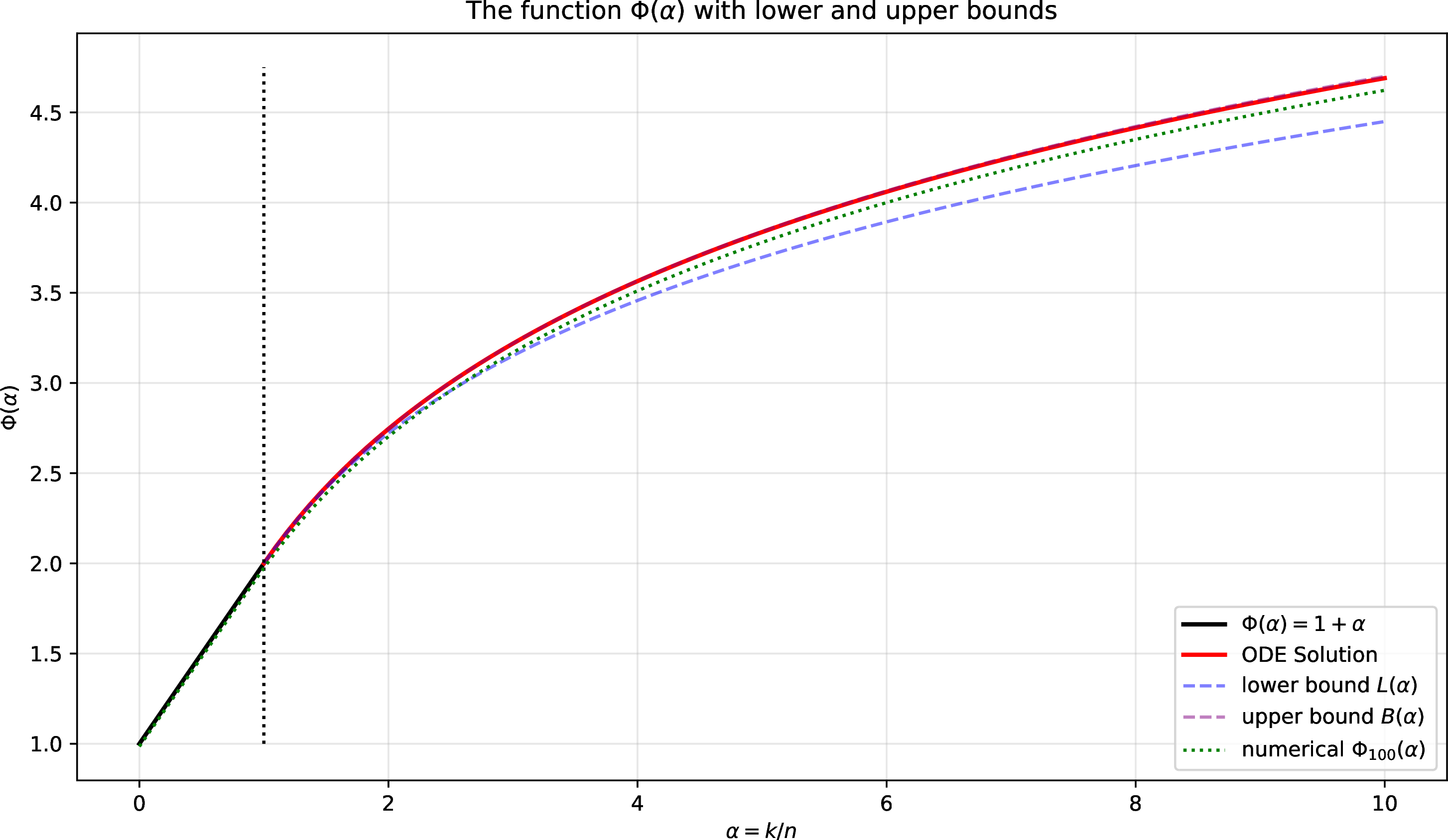
A plot depicting the functions \(\Phi(\alpha)\) and its lower and upper bounds \(L(\alpha)\) and \(B(\alpha)\) is given in Figure 3. The values of \(\Phi(\alpha)\) were obtained by numerically solving the differential equation defining \(\Phi(\alpha)\). As claimed, \(L(\alpha)\) is a lower bound, and \(B(\alpha)\) is an upper bound on \(\Phi(\alpha)\). The upper bound \(B(\alpha)\) seems to be extremely tight, at least for \(\alpha\le 10\). Also shown in the plot, as a dotted green line, is the empirical function \(\tilde{\Phi}_{100}(\alpha) = \left(\frac{\ln F(n,\alpha n)}{2\sqrt{n}}\right)^2\), for \(n=100,000\). As expected, this function lies below \(\Phi(\alpha)\), consistent with the upper bound claim. The small gap between \(\tilde{\Phi}_{100}(\alpha)\) and \(\Phi(\alpha)\) is explained by the hypothesis that \(F(n,\alpha n)\) is asymptotically of the form \((n(1+\alpha))^{A}\,e^{2\sqrt{n\Phi(\alpha)}}\) for some constant \(A<0\). Choosing \(A=-\frac{1}{2}\) yields an almost perfect fit. The choice \(A=-\frac{1}{2}\) is also supported by some heuristic calculations that we do not repeat here. The factor \(n+k\) used in our upper bound proof, which corresponds to the choice \(A=1\), was added to simplify the proof. Proving that the \(n+k\) factor can possibly be replaced by a \((n+k)^{-1/2}\) would require a more complicated analysis that would use more terms in the Taylor expansions used in the current proof.

19.5 Concavity of \(\Phi\)↩︎

To prove the strict concavity of \(\Phi(\alpha)\) for \(\alpha>1\), we prove that \(\Phi''(\alpha)<0\), for \(\alpha>1\). Recall that \(\Phi\) satisfies Equations 1 and 2 from Section 8: \[\alpha (\Phi')^2 - \Phi \Phi' + \frac{\Phi}{1+\alpha} \;=\;0 \quad,\quad \Phi' \;=\;\frac{\Phi - D}{2\alpha} \quad,\quad D \;=\;\sqrt{\Phi^2 - \frac{4\alpha\Phi}{1+\alpha}} \;.\] Differentiating the first equation with respect to \(\alpha\) yields: \[(\Phi')^2 + 2\alpha\Phi'\Phi'' - \left(\Phi'\Phi' + \Phi\Phi''\right) + \frac{\Phi'(1+\alpha) - \Phi}{(1+\alpha)^2} \;=\;0 \;.\] After simplifying we get: \[\Phi''(2\alpha\Phi' - \Phi) \;=\;\frac{\Phi - (1+\alpha)\Phi'}{(1+\alpha)^2} \;.\] Note that \(2\alpha\Phi' - \Phi=-D<0\), for \(\alpha>1\). To finish the proof, note that \[\Phi - (1+\alpha)\Phi' \;=\;\Phi - (1+\alpha) \frac{\Phi - D}{2\alpha} \;=\;\frac{\alpha-1}{2\alpha}\Phi + \frac{1+\alpha}{2\alpha}D \;>\;0\;,\] as both \(\Phi>0\) and \(D>0\), for \(\alpha>1\).

20 Partial derivatives of \(S(n,k)\)↩︎

We give the explicit computation of \(S_n\) and \(S_k\). The computations of \(S_{nn}\) and \(S_{kk}\) are similar. Recall that \(S(n,k)=2\sqrt{n\Phi(\alpha)}=2\sqrt{n\Phi(\frac{k}{n})}\). As before, we use the shorthands \(\Phi=\Phi(\alpha)\) and \(\Phi'=\Phi'(\alpha)\).

Using the chain rule and \(\frac{\partial \alpha}{\partial k} = \frac{1}{n}\), we have \[S_k \;=\;\frac{\partial}{\partial k} \left( 2\sqrt{n} \sqrt{\Phi} \right) \;=\;2\sqrt{n} \cdot \frac{1}{2\sqrt{\Phi}} \cdot \Phi' \cdot \frac{1}{n} \;=\;\frac{\Phi'}{\sqrt{n \Phi}} \;.\] Using \(\frac{\partial \alpha}{\partial n} = -\frac{k}{n^2} = -\frac{\alpha}{n}\), we have \[\begin{align} S_n &\;=\;\frac{\partial}{\partial n} \left( 2\sqrt{n\Phi} \right) = 2 \left( \frac{\sqrt{\Phi}}{2\sqrt{n}} + \sqrt{n} \frac{\Phi'}{2\sqrt{\Phi}} \cdot\left( -\frac{\alpha}{n} \right) \right) \\ &\;=\;\frac{\Phi}{\sqrt{n\Phi}} - \frac{\alpha \Phi'}{\sqrt{n\Phi}} \;=\;\frac{\Phi - \alpha \Phi'}{\sqrt{n\Phi}} \;. \qedhere \end{align}\]

Since \(S(n,k)\) is positively homogeneous of degree \(1/2\), i.e., \(S(tn,tk)=t^{1/2}S(n,k)\), it follows from Euler’s Theorem on Homogeneous Functions (see, e.g., Apostol [74]) that \(n S_n + k S_k = \frac{1}{2}S = \sqrt{n\Phi}\), as we can also verify directly.

21 The concavity of \(S(n,k)\)↩︎

Recall that \[S_{nn} \;=\;\frac{\alpha^2 \Phi \Phi'' - \frac{1}{2}(\Phi - \alpha\Phi')^2}{(n\Phi)^{3/2}} \quad,\quad S_{kk} \;=\;\frac{\Phi \Phi'' - \frac{1}{2}(\Phi')^2}{(n\Phi)^{3/2}} \;.\] For \(\alpha>1\) we have \(\Phi>0\) and \(\Phi''<0\). We also have \((\Phi - \alpha\Phi')^2\ge 0\) and \((\Phi')^2\ge 0\), Thus \(S_{nn}<0\) and \(S_{kk}<0\), as required.

References↩︎

---

1. Blavatnik School of Computer Science, Tel Aviv University, Israel. E-mail: zwick@tau.ac.il. Work supported by ISF grant no. 2854/20.↩︎