Dithered Gaussian Mechanism for Randomness-Efficient Differential Privacy
July 07, 2026
Abstract
We present the dithered Gaussian mechanism, a novel alternative to the discrete Gaussian mechanism for differential privacy that discretizes the private output rather than the noise distribution itself. By interpreting this discretization as post-processing of the Gaussian mechanism, our construction directly inherits the privacy guarantees of the standard Gaussian mechanism while avoiding vulnerabilities caused by finite-precision floating-point outputs. We show that the mechanism is provably randomness-efficient: by sampling the discretized output values directly, the number of high-quality random bits required for privacy can be reduced significantly and made independent of the noise level. This is achieved by separating the randomness into two sources: a high-quality source used for the privacy-critical sampling step, and a high-performance public source, possibly known to the adversary, that supplies the additional randomness needed for randomized discretization. This separation enables the use of cryptographically secure randomness without substantial performance loss. As an application, we study model training with DP-SGD and show that cryptographically secure noise generation with reduced exposure to floating-point vulnerabilities can be achieved with modest practical overhead.
1 Introduction↩︎
Modern machine learning increasingly relies on sensitive individual-level data, making formal privacy guarantees essential. Differential privacy provides one such guarantee by limiting how much any single data point can influence the output of an algorithm. The Gaussian mechanism [1] is one of the most widely used primitives for ensuring differential privacy. It is especially central in private machine learning, where it forms the noise-addition step of differentially private stochastic gradient descent (DP-SGD) [2]. Despite its ubiquity, the Gaussian mechanism has important practical limitations. First, it is an idealized continuous mechanism, whereas real implementations run on finite-precision computers. As a result, a faithful implementation of a continuous Gaussian distribution is impossible: naive samplers can leave detectable “holes” in the set of representable floating-point values, creating privacy vulnerabilities of the kind first observed for the Laplace mechanism [3] and later identified for the Gaussian mechanism itself [4]. A second limitation is the amount of randomness required to sample Gaussian noise. In the ideal continuous model, exact sampling requires infinitely many random bits, while high-precision implementations can still require many random bits in practice. This cost becomes substantial at scale: recent efforts to train language models entirely under differential privacy, such as the VaultGemma 1B model, required quadrillions of Gaussian random draws and petabytes of randomness to obtain a formal privacy guarantee [5]. At this scale, randomness generation itself can become a bottleneck [6]. Several discrete-valued mechanisms, most prominently the discrete Gaussian mechanism [7], address finite-precision concerns by adding discrete noise. However, these mechanisms can still require many privacy-critical random bits. Moreover, because their privacy guarantees do not directly follow from those of the continuous Gaussian mechanism, they require separate privacy analyses for composition and amplification by subsampling, making them difficult to use as drop-in replacements for Gaussian noise in DP-SGD. Unlike existing discrete mechanisms, which approximate Gaussian noise and typically require separate privacy analyses, our construction inherits the privacy guarantees of the standard Gaussian mechanism directly, making it compatible with existing Gaussian-based analyses. At the same time, the mechanism avoids vulnerabilities arising from finite-precision floating-point representations and is provably randomness-efficient, improving on prior efficient constructions. Finally, we apply the mechanism to DP-SGD and show that it enables cryptographically secure noise generation with reduced floating-point vulnerabilities and a modest time overhead. Compared with methods that use floating-point Gaussian noise sampled from pseudorandom number generators without cryptographic guarantees, our method incurs an overhead of about \(30\%\), and only about \(20\%\) when compared with cryptographically secure noise generation in experiments on CIFAR-10.
1.0.0.1 Our contributions.
We propose a drop-in replacement for the Gaussian mechanism that is cryptographically secure, resistant to floating-point attacks, and time-efficient. This is achieved with a novel approach to noise addition that we call the dithered Gaussian mechanism. The mechanism is defined through the distribution of a rounded, dithered Gaussian output: we consider the value that would be obtained by adding Gaussian noise to the sensitive vector, adding a public random offset, or dither, and rounding the result to a discrete grid determined by the same public offset. Crucially, this discrete output distribution can be written down explicitly after conditioning on the dither, and our mechanism samples from it directly using high-quality private randomness, rather than sampling the intermediate continuous Gaussian noise. The key observation is that the rounded output is a post-processing of the standard Gaussian mechanism, so it directly inherits the privacy guarantees of the Gaussian mechanism. The public dither is not needed for privacy, but improves the quality of the discretization and helps reduce the amount of private randomness required for direct sampling. In particular, we show that the number of private random bits can be made independent of the Gaussian noise scale, without significantly changing the distribution of the perturbation relative to the Gaussian mechanism. This substantially reduces the cost of using cryptographically secure randomness. Since the released output is discrete by construction (conditioned on the public dither), the mechanism avoids finite-precision issues associated with floating-point outputs. Finally, we apply the mechanism to DP-SGD and show that it enables cryptographically secure private randomness with modest practical overhead.
1.1 Related work↩︎
1.1.0.1 Floating-point vulnerabilities and discrete mechanisms.
A subtle but important issue in the implementation of differentially private mechanisms is the use of finite-precision floating-point arithmetic. Mironov [3] showed that naive implementations of the Laplace mechanism can leave detectable “holes” in the set of representable noisy outputs, which can be sufficient to reconstruct a significant part of the underlying data. Similar finite-precision issues have since been identified for other mechanisms, including the exponential mechanism [8], Noisy Max [9], and the Gaussian mechanism [4]. A related class of attacks exploits precision-dependent leakage: the precision of the released noisy value may depend on the exponent of the original value, thereby leaking information about the input [10]. Several implementation-level mitigations have been proposed [10], [11] and adopted in practical differential privacy libraries, including diffprivlib [12], OpenDP [13], and the “secure mode” of Opacus [14]. These approaches improve the robustness of floating-point implementations, but they do not remove the underlying mismatch between continuous idealized mechanisms and finite-precision computation.
A more direct way to avoid this kind of vulnerability is to work only with values from a discrete domain. Several discrete-valued mechanisms have been proposed for this purpose, including the discrete Laplace mechanism, also known as the geometric mechanism [15]; the discrete Gaussian mechanism [7]; the binomial mechanism [1], [16]; and mechanisms based on Poisson random variables, such as the Skellam mechanism [17], the Skellam Mixture Mechanism [18], and the Poisson Binomial Mechanism [19]. By adding discrete noise and releasing discrete outputs, these mechanisms avoid the floating-point artifacts described above. However, they have two important limitations from the perspective of our work. First, they can still require substantial amounts of randomness for noise generation, unless one uses coarse approximations. Second, mechanisms such as the discrete Gaussian, Skellam, and binomial mechanisms approximate Gaussian noise but do not automatically inherit the privacy guarantees of the continuous Gaussian mechanism. Consequently, analyses for composition, amplification by subsampling, or other accounting procedures generally have to be established separately.
1.1.0.2 Randomness complexity.
From a theoretical standpoint, the large randomness requirements of practical differentially private algorithms raise a natural question at the intersection of privacy and complexity: how much randomness is actually necessary for privacy? Canonne, Su, and Vadhan [20] initiated the study of the randomness complexity of differential privacy, showing that highly accurate private mechanisms can sometimes be implemented with surprisingly few random bits, in some settings as few as logarithmically many in the number of released statistics. This contrasts with the common intuition that the randomness required for privacy should scale with the dimension of the output. Their construction is based on a connection to secluded partitions from computational geometry [21], but is not computationally efficient. More recently, Ghentiyala [22] gave a computationally efficient alternative, at the cost of a polylogarithmic loss in the randomness-error trade-off. While both approaches are theoretically interesting, we are not aware of any demonstrations of their practical value.
1.1.0.3 DP-SGD and discrete mechanisms.
One of the most important applications of Gaussian noise in differential privacy is the training of machine learning models, most commonly through differentially private stochastic gradient descent (DP-SGD) [2], [23], [24]. The privacy guarantees of DP-SGD are typically established using privacy accountants that exploit the structure of the sampling procedure, including Poisson subsampling [2], [25]–[28], shuffling [29]–[32], sampling without replacement [33], [34], and random allocations such as Balls-in-Bins [35], [36]. Many of these analyses are developed specifically for the Gaussian mechanism, making it difficult to replace Gaussian noise with a different noise distribution without redoing the privacy analysis. Discrete mechanisms have also been studied in combination with DP-SGD, especially in federated learning with secure aggregation [16]–[19], [37]. In this setting, the main goals are to obtain integer-valued noisy gradient sums, which integrate naturally with secure aggregation, and to reduce communication complexity. To the best of our knowledge, however, tight analyses of subsampled discrete mechanisms are not available even for the standard Poisson subsampling scheme. Existing approaches therefore typically start from concentrated DP or Rényi DP guarantees for the underlying discrete mechanism, combine them with a generic subsampling amplification lemma, and then apply generic composition within the chosen privacy framework, as in [17], [37]. This contrasts with our approach, where the discretized mechanism inherits Gaussian privacy guarantees by post-processing and can therefore reuse Gaussian-based analyses directly.
2 Background↩︎
In this section, we first introduce the notions of sensitivity, randomness complexity, and privacy that will be used throughout the paper. Second, we present the properties of the discrete Gaussian mechanism with respect to these notions.
Sensitivity. Consider datasets \(X\) that are finite subsets of some set \(\mathbb{X}\). We work in the add/remove adjacency notion: two datasets \(X\sim X'\) are neighbors if one can be obtained from the other by inserting or deleting a single data point. For a dataset of \(n\) elements we write its elements as \(X=\{x^{(1)},\ldots,x^{(n)}\}\subseteq\mathbb{X}\). For \(p\geq 1\), the global \(\ell_p\)-sensitivity of a function \(f:\mathbb{X}^*\rightarrow\mathbb{R}^d\) is defined as \[\Delta_p(f)\;:=\;\sup_{X\sim X'} \|f(X)-f(X')\|_p.\]
Randomness complexity. The randomness complexity of \(\mathcal{M}\) is the expected number of random bits required to produce an output of the mechanism. As noted by Canonne, Su, and Vadhan [20], this quantity is tightly linked, up to an additive constant, to the Shannon entropy of the mechanism. When running a sequence of mechanisms independently (keeping public randomness fixed), the total private randomness complexity can be bounded by the sum of entropies plus an additive constant.
Differential privacy. We can release an estimate of \(f(X)\) while satisfying differential privacy by adding noise to \(f(X)\) scaled according to the sensitivity. Intuitively, differential privacy means that the information released has roughly the same distribution for neighboring datasets \(X\) and \(X'\). For example, the Laplace mechanism (for \(p=1\)) attains \((\varepsilon,0)\)-differential privacy and the Gaussian mechanism (for \(p=2\)) attains \((\varepsilon,\delta)\)-differential privacy. We refer to Appendix 6 for definitions of differential privacy and properties of basic noise addition mechanisms.
Discrete Gaussian mechanism. Traditionally, differential privacy has been analyzed under the idealized assumption that mechanisms have access to samples from continuous distributions. Under this viewpoint, the amount of randomness required by a mechanism is typically not accounted for explicitly, and no finite upper bound on the number of random bits is established. In practice, however, implementations must operate on finite-precision computers and therefore rely on discrete distributions or finite procedures for sampling. This issue has been studied, for example, by Balcer and Vadhan [38] and by Canonne, Kamath, and Steinke [7], who show that discrete analogues of standard private mechanisms admit finite bounds on the required randomness. A canonical example is the discrete Gaussian mechanism [7], which replaces continuous Gaussian noise with noise drawn from a discrete distribution over the integers with probabilities derived from the density of a Gaussian. Besides being implementable on finite computers, this mechanism provides a natural starting point for studying the randomness complexity of differentially private algorithms.
Definition 1 (Discrete Gaussian mechanism). Let \(f : \mathcal{X}^n \to \mathbb{Z}^d\) be a function with sensitivity \(\Delta_2(f)\). For \(\sigma_{} > 0\), the discrete Gaussian mechanism with scale \(\sigma \Delta_2(f)\) releases \[M(x) = f(x) + Z,\] where \(Z = (Z_1,\dots,Z_d) \in \mathbb{Z}^d\) has independent coordinates, and each \(Z_j\) is sampled from the one-dimensional discrete Gaussian distribution centered at \(0\) with scale \(\sigma \Delta_2(f)\), that is, \[\mathbb{P}(Z_j = z) = \frac{\exp\!\left(-\frac{z^2}{2\sigma^2 \Delta_2(f)^2}\right)}{\sum_{u \in \mathbb{Z}} \exp\!\left(-\frac{u^2}{2\sigma^2 \Delta_2(f)^2}\right)} \qquad \text{for all } z \in \mathbb{Z}.\]
Discretization. Note that the discrete Gaussian mechanism is defined only for integer-valued functions. To apply it to general real-valued functions, one must first discretize the values of \(f\). Let \(f(x) \in \mathbb{R}^d\) have sensitivity \(\Delta_2(f)\), and let \(h > 0\) be a discretization parameter. If each coordinate is rounded to the nearest integer multiple of \(h\), then the sensitivity of the discretized function \(\tilde{f}\) satisfies \[\label{eq:sensitivity95rounding} \Delta_2(\tilde{f}) \le \Delta_2(f) + \frac{h\sqrt{d}}{2}.\tag{1}\] However, such deterministic rounding introduces bias. Randomizing the decision whether to round up or down removes this bias, but increases the sensitivity to \(\Delta_2(f) + h\sqrt{d}\). A better trade-off can be obtained by allowing a resampling probability \(\beta \in (0,1)\), resulting in a small bias, as described by Kairouz, Liu, and Steinke [37]. They use a random rotation technique to ensure that, with high probability, the sensitivity of the rounded vector is bounded by \[\tilde{\Delta}_2(f) \le \min\left\{ \Delta_2(f) + h\sqrt{d},\, \sqrt{\vphantom{\frac{\sqrt{d}h^2}{2}} \Delta_2^2(f) + \frac{dh^2}{4} + \sqrt{2\ln(1/\beta)} \left( \Delta_2(f)h + \frac{\sqrt{d}h^2}{2} \right) } \right\}.\] To guarantee privacy, the rotation must be repeated until the required condition on the \(\ell_2\) norm is satisfied.
Randomness complexity of the discrete Gaussian. The choice of discretization parameter \(h\) creates a tension for the discrete Gaussian mechanism because the noise must be generated on the lattice \(h\mathbb{Z}^d\). Equivalently, one may first scale the function by \(1/h\), round and apply the discrete Gaussian mechanism on \(\mathbb{Z}^d\), and then rescale the output by multiplying with \(h\). If \(\sigma > 0\) is the noise level required by the Gaussian mechanism for differential privacy, then the corresponding discrete mechanism uses scale \(\tau = \sigma \Delta_2(\tilde{f})/h\), before the resulting noise is ultimately rescaled by \(h\). The variance of the resulting mechanism is close to that of the continuous Gaussian mechanism provided that \(h \ll \Delta_2(f)/\sqrt{d}\). However, even in the regime where the variance increase is small, the entropy increases significantly as \(h\) approaches \(0\). In particular, the binary entropy of \(Z_j\) sampled from the one-dimensional discrete Gaussian distribution with scale \(\tau\) is \[H(Z_j)=\frac{1}{2}\log_2(2\pi e\,\tau^2)+o_\tau(1),\] see Lemma 6 of [39]. Since the coordinates of \(Z=(Z_1,\dots,Z_d)\) are independent, it follows that the binary entropy of the \(d\)-dimensional discrete Gaussian is \[H(Z)=\sum_{j=1}^d H(Z_j)=\frac{d}{2}\log_2(2\pi e\,\tau^2)+o_\tau(d).\] With \(\tau = \sigma \Delta_2(\tilde{f})/h\) this is approximately \(d\log_2\!\left(\frac{\sigma \Delta_2(\tilde{f})}{h}\right) + 2d\) for large enough \(d\). We note that this bound is not tight for the case where \(h\) is large compared to \(\sigma \Delta_2(\tilde{f})\), where in fact the entropy can be \(o(d)\).
3 Dithered Gaussian Mechanism↩︎
We now present an alternative to the discrete Gaussian that avoids the need to discretize the input. Unlike the methods described in Section 2 it does not incur any increase in sensitivity. Moreover, our method uses provably fewer random bits, making it practical even when noise must be generated using slow cryptographically secure randomness. In addition, the method directly inherits the privacy guarantees of the (continuous) Gaussian mechanism, and therefore does not require separate proofs for composition or amplification by subsampling.
Conceptual description. Our method, the dithered Gaussian mechanism, is illustrated in Figure 1. It can be thought of as a post-processing of the Gaussian mechanism with noise scale \(\sigma\), i.e., the mechanism that outputs \(f(X)+y\), where \(y\sim\mathcal{N}(0,\sigma^2 I_d)\). The post-processing simply rounds each coordinate to an axis-aligned grid of points with distance \(\xi>0\) between consecutive points along all axes. Performing this rounding deterministically would introduce bias, but we avoid this with a random shift of the grid: Sample public randomness \((a,b)\sim \mathrm{Uniform}([0,1)^2)\) and define the coordinate-dependent dither by \(\gamma_i=(ai+b)\bmod 1\) for each \(i\in[d]\). Given \(f(X)\in\mathbb{R}^d\) and \(y\sim\mathcal{N}(0,\sigma^2 I_d)\), the mechanism outputs \(\mathcal{M}(f(X))\) where, for \(i=1,\dots,d\), \[\label{eq:mechanism} \mathcal{M}(f(X))_i = \xi\left( \left\lfloor \frac{f(X)_i+y_i}{\xi}-\gamma_i+\frac{1}{2} \right\rfloor +\gamma_i \right).\tag{2}\]
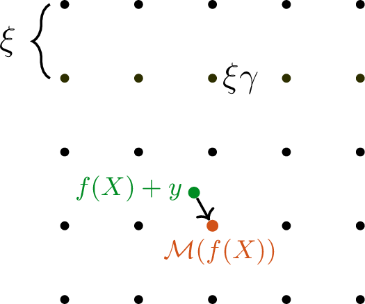
Direct sampling from a discrete distribution. To avoid generating the Gaussian vector \(y\) we observe that it is possible to sample the integer-valued random variable \[Z_i := \left\lfloor \frac{f(X)_i+y_i}{\xi}-\gamma_i+\frac{1}{2} \right\rfloor\] directly without first sampling \(y_i\). Indeed, for each \(k\in\mathbb{Z}\), the event \(Z_i=k\) is equivalent to \[k \le \frac{f(X)_i+y_i}{\xi}-\gamma_i+\tfrac12 < k+1 \Leftrightarrow \frac{\xi\left(k+\gamma_i - \frac{1}{2}\right)-f(X)_i}{\sigma} \leq \frac{y_i}{\sigma} < \frac{\xi\left(k+\gamma_i + \frac{1}{2}\right)-f(X)_i}{\sigma}.\] Denoting the cumulative distribution function of \(\frac{y_i}{\sigma}\sim\mathcal{N}(0,1)\) by \(\Phi\) we thus have: \[\label{eq:Z95k} \Pr[Z_i=k] = \Phi\!\left( \frac{\xi\left(k+\gamma_i+\frac{1}{2}\right)-f(X)_i}{\sigma} \right) - \Phi\!\left( \frac{\xi\left(k+\gamma_i-\frac{1}{2}\right)-f(X)_i}{\sigma} \right), \qquad k\in\mathbb{Z}.\tag{3}\] Since \(\mathcal{M}(f(X))_i=\xi(Z_i+\gamma_i)\), this shows that to compute \(\mathcal{M}(f(X))_i\) it suffices to sample directly from a discrete distribution over \(\mathbb{Z}\).
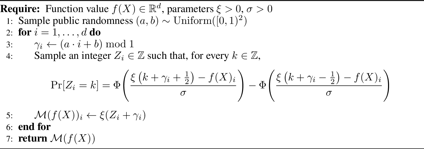
Algorithm details. We summarize the algorithm implementation in Algorithm 2. This abstract description uses real-valued variables and functions to determine sampling probabilities for the random variable \(Z_i\). In theory it is possible to generate samples from the distribution of \(Z_i\) exactly even on a finite computer using a standard technique: Compute values only to the precision needed for a sample. For example, one may first propose a finite range of candidate integer values \(k\in\mathbb{Z}\) together with a target precision for the computation of the probabilities \(\Pr[Z_i=k]\). One then samples a uniform random variable from \([0,1)\) and uses the computed probability masses to locate the corresponding outcome. If the sampled value falls within the unresolved numerical precision margin, or within the probability mass of the truncated tail, the range of candidate values and the precision of the probability computation can be refined, for example by doubling both, and the procedure repeated. While exact sampling is thus possible in principle, such a procedure appears difficult to implement efficiently in practice, especially in the setting of model training on GPUs within existing machine learning frameworks. For this reason, we instead use an approximate, randomness-efficient sampling procedure based on high-probability interval truncation and arithmetic coding. Details can be found in Appendix 7. This approach is vectorizable and can be efficiently implemented in PyTorch.
Noise distribution. We characterize the distribution of \(\mathcal{M}(X)\) over the random choice of \(\gamma\) and \(Z\):
lemmaditheredGaussianRoundingLemma Over the randomness of the shift \(\gamma_i\) and index \(Z_i\), \(\mathcal{M}(f(X))_i\) is identically distributed to \[f(X)_i + y_i + u_i,\] where \(u_i \sim \mathrm{Uniform}(-\xi/2,\xi/2)\) and \(y_i\sim\mathcal{N}(0,\sigma^2)\) are independent.
The lemma is a consequence of the fact that the grid shift \(\gamma_i\) is uniformly distributed and independent of the Gaussian noise \(y_i\), which causes the perturbation caused by rounding to the nearest grid point to follow a uniform distribution on \((-\xi/2,\xi/2)\). The full proof is provided in Appendix 9.
From a utility perspective, the dithered Gaussian mechanism is therefore equivalent to adding Gaussian noise \(\mathcal{N}(0,\sigma^2)\) and uniform noise \(\mathrm{Uniform}(-\xi/2,\xi/2)\). The variance of the resulting noise is \[\mathrm{Var}(y_i + u_i) = \sigma^2 + \xi^2/12.\]
The density of the resulting noise distribution is \[p_{y_i + u_i}(t) = \frac{1}{\xi} \left[ \Phi\left(\frac{t+\xi/2}{\sigma}\right) - \Phi\left(\frac{t-\xi/2}{\sigma}\right) \right].\]
Integrating the density by parts, we obtain an expression for the cumulative distribution function of the noise introduced by the dithered Gaussian mechanism. Using \(\phi\) to denote the standard Gaussian density: \[\begin{align} F_{y_i+u_i}(t) = \frac{1}{\xi} \Bigg[ &\left(t+\frac{\xi}{2}\right) \Phi\!\left(\frac{t+\xi/2}{\sigma}\right) + \sigma \phi\!\left(\frac{t+\xi/2}{\sigma}\right) \notag\\ &- \left(t-\frac{\xi}{2}\right) \Phi\!\left(\frac{t-\xi/2}{\sigma}\right) - \sigma \phi\!\left(\frac{t-\xi/2}{\sigma}\right) \Bigg]. \end{align}\]
We can also quantify directly how close this noise distribution is to the Gaussian distribution used by the standard Gaussian mechanism in terms of the total variation distance.
propositionditheredGaussianTVBound Let \(G_\sigma\sim\mathcal{N}(0,\sigma^2)\), and let \(U_\xi\sim\mathrm{Uniform}(-\xi/2,\xi/2)\) be independent of \(G_\sigma\). Then \[\label{eq:dithered95gaussian95tv95bound} d_{\mathrm{TV}}(G_\sigma+U_\xi,G_\sigma) \le 0.0202 \left(\frac{\xi}{\sigma}\right)^2.\tag{4}\]
Thus the distributional error introduced by dithering is quadratic in the relative grid width \(\xi/\sigma\). For a \(d\)-dimensional mechanism with independent coordinates, the corresponding product-distribution distance is at most \(0.0202\,d(\xi/\sigma)^2\) by a standard coupling bound.
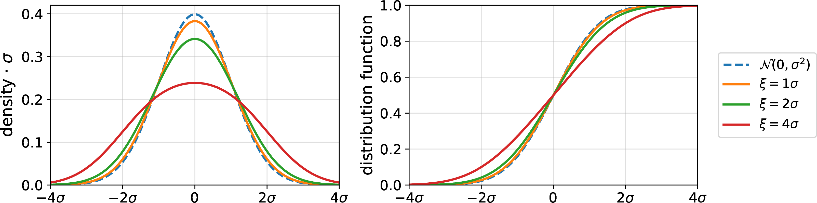
Densities for dithered Gaussians for various choices of \(\xi\) can be seen in Figure 3. For \(\xi = \sigma\) we see that the density is nearly indistinguishable from that of the standard Gaussian, while larger values of \(\xi\) somewhat flatten the distribution.
Randomness complexity. Next, we analyze the randomness complexity of the dithered Gaussian mechanism. We distinguish between the private (high-quality) randomness used for discrete sampling and the public randomness used to generate the pair \((a, b)\) of uniform random variables defining the grid shift \(\gamma\). The value \(\gamma\) may be shared with the adversary without compromising privacy, its purpose is solely to improve utility.
We bound the entropy of the dithered Gaussian mechanism in the following lemma:
lemmaditheredGaussianEntropyBound The worst-case private binary entropy of the dithered Gaussian mechanism is bounded by \[H(Z\mid \gamma) \le \frac{d}{2}\log_2\left( 2\pi e\left[ \left(\frac{\sigma}{\xi}+\frac{1}{2}\right)^2+\frac{1}{12} \right] \right).\]
The full proof is given in Appendix 9.
As noted above one can choose \(\xi \approx \sigma\) and get an error distribution that is close to Gaussian. In this case, the lemma says that the entropy per coordinate is a small constant. More precise plots of the entropy are shown in Figure 4. Intuition for why this mechanism has low entropy, in expectation over the randomness of \(\gamma_i\), is that for large enough \(\xi\), the random noise \(y_i\) is unlikely to make \(\mathcal{M}(f(X))_i\) differ from the output with fixed \(y_i = 0\). Thus each coordinate is close to deterministic in expectation, which implies low entropy. This argument extends and refines similar observations by Ghentiyala [22]. In theory, using techniques for sampling from low-entropy distributions based on explicit, ordered sampling probabilities [40], [41], multiple runs of the mechanism can be implemented in time near-linear in \(d\) using an expected number of random bits that matches the sum of all private entropy bounds plus \(O(\log(1/\beta))\) bits with probability \(1-\beta\). As mentioned above, details of the implementation of our sampling mechanism can be found in Appendix 7.
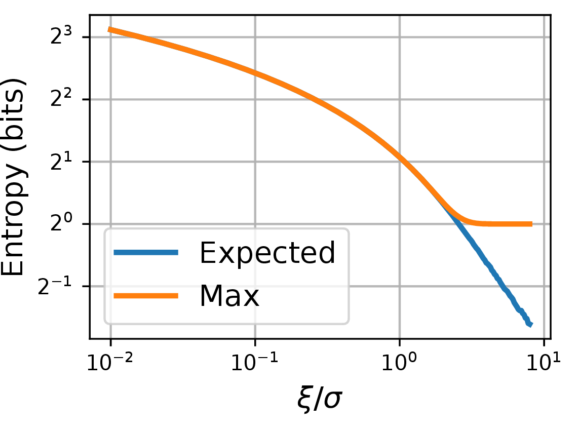
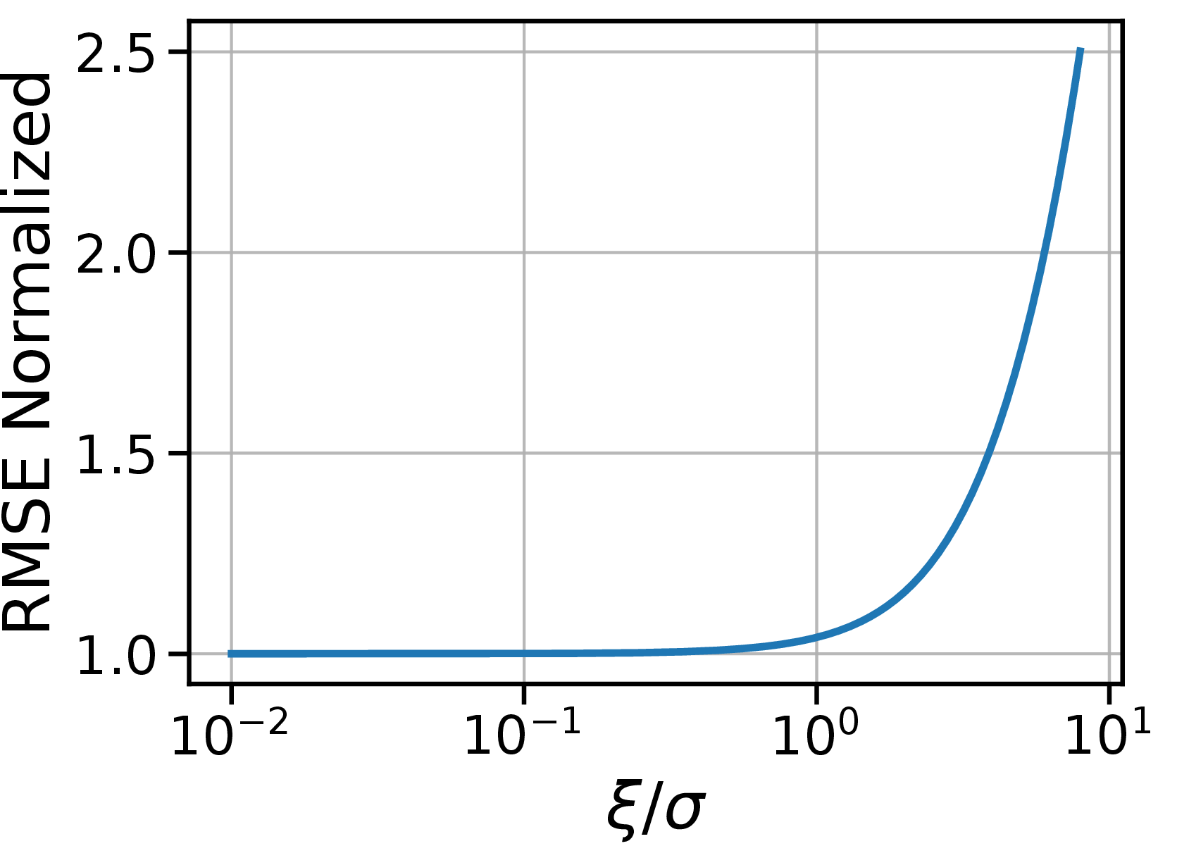
Figure 4: The expected and maximum entropy (a) and normalized RMSE of the dithered Gaussian mechanism (b) as functions of \(\xi / \sigma\).. a — Entropy of the dithered Gaussian distribution., b — Root mean squared error normalized by \(\sigma\).
3.1 Comparison to the mechanism of Ghentiyala↩︎
Ghentiyala [22] recently proposed an efficient derandomization method for differentially private summation that, like our approach, relies on adding noise followed by a random grid shift and rounding. Both constructions exploit the fact that, after a suitable random shift, we expect only a small subset of coordinates to be “ambiguous” in the sense that their rounded values are likely to depend on the value of the added noise vector \(y\). While our analysis relies on entropy, Ghentiyala’s construction uses discrete Laplace or Gaussian noise and achieves efficiency by selectively sampling noise only on coordinates whose values might change after rounding. This results in multiplicative polylogarithmic factors in the expected randomness complexity, making it higher than that of [20] and ours. Unlike our pairwise independent offset vector \(\gamma\), Ghentiyala uses the same random offset for every coordinate. A consequence of this is that even though the expected randomness complexity is similar to that of [20], the variance in the number of random bits can be much higher than in the construction of [20] as well as ours. Like our construction, Ghentiyala’s is explicit and computationally efficient. Though no attempt is made in [22] to distinguish between public and private randomness complexity, it seems that the randomness used for the shift can be made public without affecting privacy.
3.1.0.1 Lower Bound.
In Appendix 8, we prove the following lower bound on the private entropy of any differentially private mechanism for releasing a sensitivity-\(C\) statistic. To make the binary entropy well-defined we consider the special case where the statistic is integer-valued. Inputs \(z\) and \(z'\) are considered neighboring if \(|z-z'|\le C\) where \(C\in\mathbb{N}\). Let \(U\) denote the public randomness, and write \(\mathcal{M}_U\) for the mechanism obtained after conditioning on \(U\).
theoremmainlower There are absolute constants \(c,c_0>0\) such that for \(\varepsilon\in(0,1)\) and \(\delta\le c_0\varepsilon\) the following holds. Suppose \(\mathcal{M}_U: \mathbb{Z}\to \mathbb{Z}\) is an \((\varepsilon,\delta)\)-differentially private mechanism under sensitivity \(C\), for every fixed value of public randomness \(U\). If, for some \(\alpha\in\mathbb{N}\) and \(\beta\in(0,\tfrac{1}{10})\), for every \(z\in\mathbb{Z}\) it holds that \(\Pr_{U,R}\!\left[|\mathcal{M}_U(z)-z|>\alpha\right]\le \beta\) (where \(R\) is the private randomness) then there exists \(z\in \mathbb{Z}\) such that \[\mathbb{E}_U\!\big[\,H(\mathcal{M}_U(z))\,\big] \ge c\,\frac{C}{\varepsilon\,\alpha}.\]
The proof proceeds by fixing a suitable value of the public randomness and using a graph-theoretic argument based on component stability and barrier structure to derive a lower bound on the achievable accuracy. Since the Gaussian noise scale needed for privacy is proportional to the clipping radius \(C\) (up to the usual dependence on \(\varepsilon,\delta\)), this lower bound shows that the relevant scale for private entropy is the ratio between the privacy noise scale and the accuracy scale. This is consistent with Lemma [lem:dithered95gaussian95entropy95bound]: the private entropy of the dithered Gaussian mechanism depends on the dimensionless ratio \(\sigma/\xi\), where \(\sigma\) is the Gaussian noise scale and \(\xi\) is the discretization width. In particular, choosing \(\xi=\Theta(\sigma)\) gives constant private entropy per coordinate, while taking a finer grid increases the entropy only logarithmically in \(\sigma/\xi\).
3.1.0.2 Dithered Laplace mechanism.
The proposed dithering scheme can also be applied to the Laplace mechanism. In Appendix 10, we provide an additional set of results specifically for the Laplace mechanism. In particular, Theorem [thm:main95dithered95laplace] establishes an upper bound on the randomness complexity, improving on the recent result of Canonne, Su, and Vadhan [20].
4 Experiments↩︎
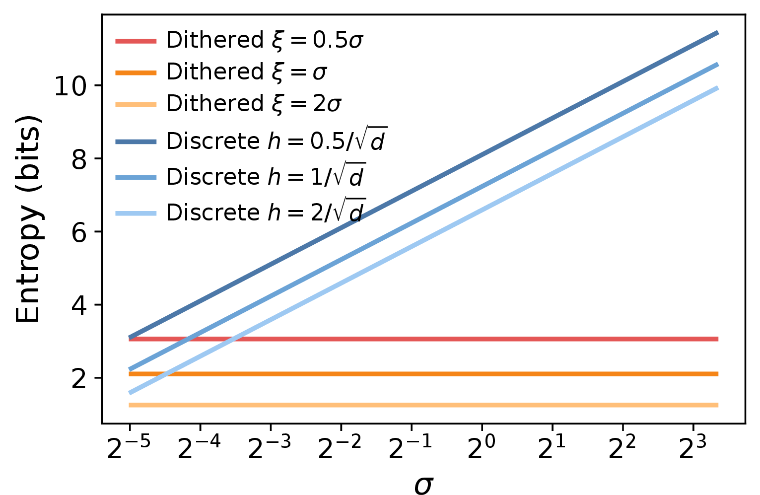
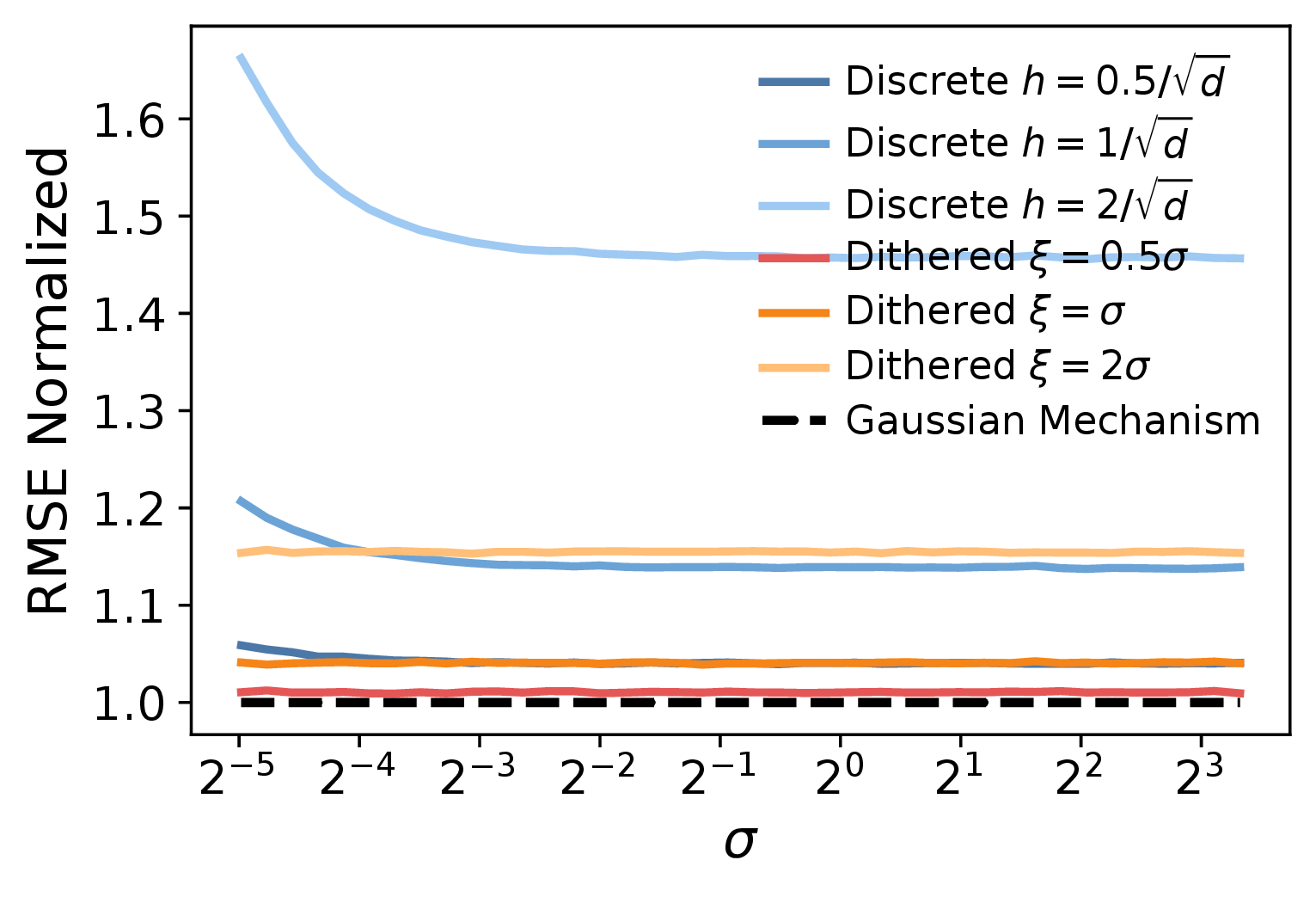
Figure 5: Comparison of the dithered and discrete Gaussian mechanisms as a function of the noise scale \(\sigma\). The left panel reports the entropy per coordinate. The right panel reports the RMSE on vectors in dimension \(d=1000\) sampled uniformly from the unit sphere. For each value of \(\sigma\), we run each mechanism \(1000\) times and compute the average reconstruction error. The RMSE is normalized by the Gaussian mechanism baseline, which is equivalent to dividing by \(\sigma\). The proposed dithered Gaussian mechanism requires a much smaller number of bits, which is independent of \(\sigma\).. a — Entropy in bits., b — Normalized RMSE.
In this section, we numerically study the utility and randomness complexity of the dithered Gaussian mechanism in comparison with the discrete Gaussian mechanism.
Entropy and RMSE. Assume that the sensitive vectors are drawn from the unit sphere in dimension \(d = 1000\). In the case of the discrete Gaussian mechanism, these vectors are further discretized with discretization levels \(h \in \{\frac{0.5}{\sqrt{d}}, \frac{1}{\sqrt{d}}, \frac{2}{\sqrt{d}}\}\). We set the resampling parameter to \(\beta = e^{-1/2}\), as suggested by Kairouz, Liu, and Steinke [37]. For the dithered Gaussian mechanism, we vary \(\xi \in \{0.5\sigma, \sigma, 2\sigma\}\). In Figure 5, we show that, for a sufficiently large noise level \(\sigma\), our method has much lower entropy and therefore requires fewer random bits to sample. In terms of utility, measured by the root mean squared error normalized by \(\sigma\), the dithered Gaussian mechanism is much closer to the Gaussian mechanism, partly because it does not require discretizing the vectors.
Model Training. We next study how the use of the dithered Gaussian mechanism affects the accuracy of DP-SGD. In Figure 6, we show the test accuracy on the CIFAR-10 dataset for different privacy budgets \(\epsilon \in \{\frac{1}{2}, 1, 2, 4, 8\}\) with \(\delta = 10^{-5}\), comparing a standard implementation of Opacus [14] that samples non-secure Gaussian noise with the dithered Gaussian mechanism for different values of \(\xi \in \{\frac{\sigma}{2}, \sigma, 2\sigma\}\). The dithered Gaussian mechanism uses cryptographically secure noise generated by the secrets module in the Python standard library [42]. We observe that the accuracy remains almost the same for \(\xi \in \{\frac{\sigma}{2}, \sigma\}\) and drops for \(\xi = 2\sigma\), which is consistent with the findings in Figures 5 and 3. The cost of using the dithered sampling scheme together with secure noise generation is an increase in training time of about \(30\%\) compared with the standard Opacus implementation of DP-SGD, and about \(20\%\) compared with Opacus’ “secure mode”, which includes cryptographically secure noise generation. However, in terms of protection against floating-point vulnerabilities and privacy accounting, secure mode should be viewed as a heuristic rather than as providing a formal guarantee.
The overhead is indicative of what one can expect in general, though the figure will depend on how much time is spent on randomness generation, which in turn depends on factors such as batch size. For instance, even when using only cryptographically secure noise, much larger overheads were observed in the work of Egan [6], ranging from \(74\%\) to over \(400\%\). In that work, a rather small batch size of \(32\) is used, making the time spent on noise generation relatively larger. It should therefore be expected that, with a much larger batch size, the overhead would drop.
Some implementation details: We trained a ConvNet model for \(10\) epochs with batch size \(512\) and clipping norm \(1\). PRV accounting was performed by Opacus, and the learning rates optimized on the validation set for each point. The time was measured on a single A100 GPU with 16 CPU cores; we report the total training time over \(10\) epochs with error bars computed over \(3\) runs.
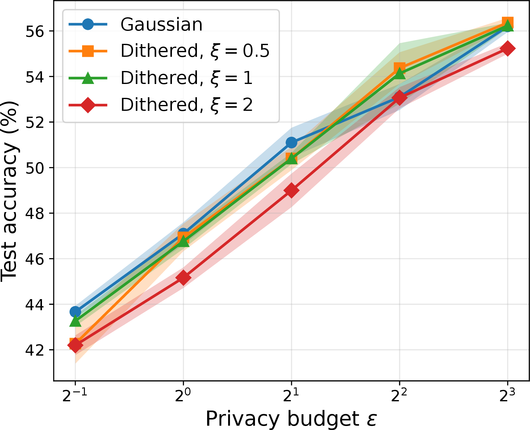
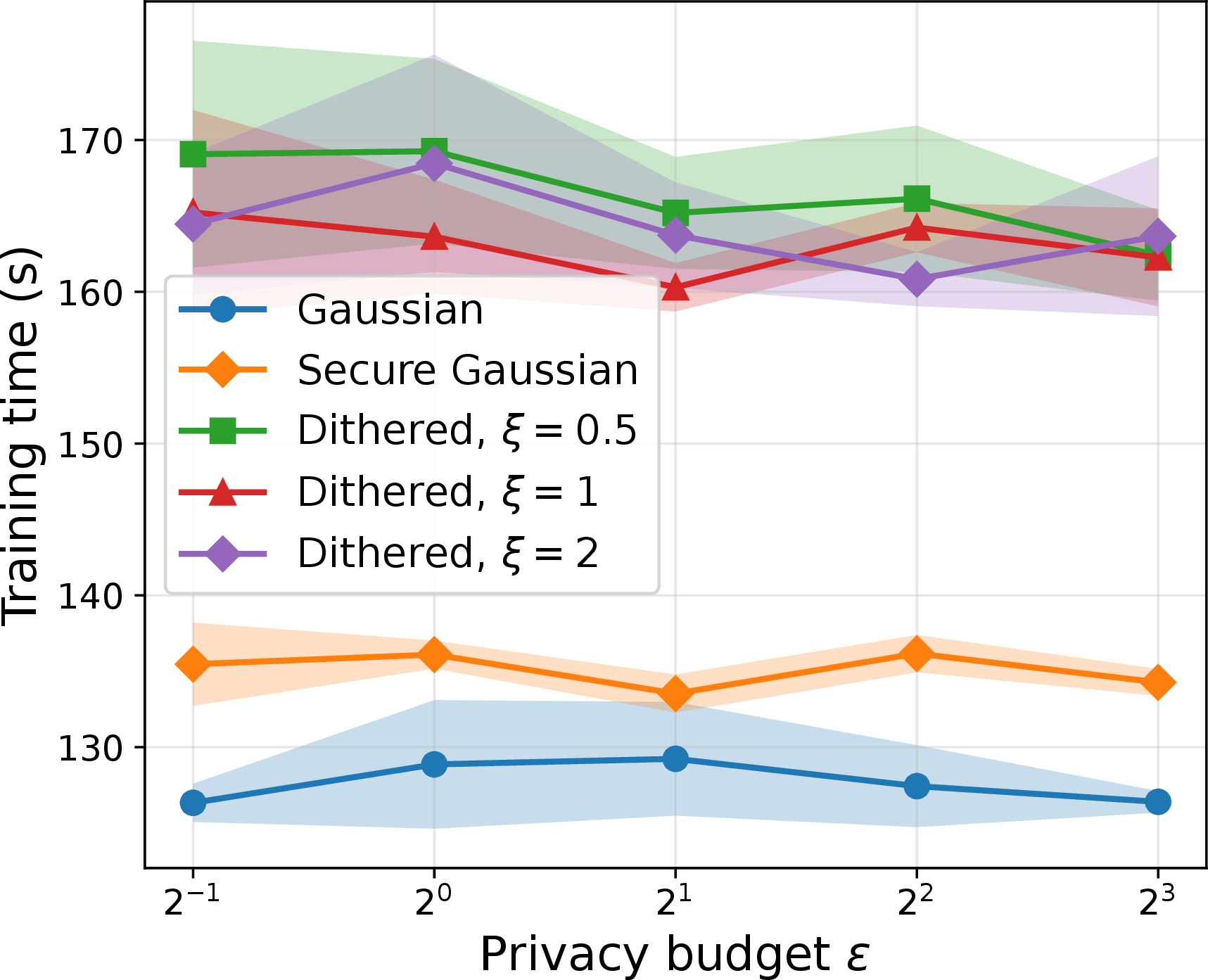
Figure 6: Comparison of Gaussian and dithered Gaussian mechanisms on CIFAR-10 across privacy budgets \(\epsilon\) with \(\delta =10^{-5}\). Solid lines show the mean over three runs, and shaded regions indicate one standard deviation. Plot (a) shows that for \(\xi = 0.5\) and \(\xi = 1\), there is no significant drop in test accuracy, whereas for \(\xi = 2\), the accuracy is substantially lower. Plot (b) shows that using the dithered Gaussian mechanism with cryptographically secure noise generation incurs a runtime increase of only about \(30\%\) compared with the standard Opacus implementation of DP-SGD, and about \(20\%\) compared with Opacus’s secure mode.. a — Test accuracy., b — Training time.
5 Conclusion and Future Directions↩︎
We have introduced the dithered Gaussian mechanism, an alternative to previous discrete noise mechanisms, which protects against floating-point vulnerabilities without requiring separate privacy accounting. Instead, it directly inherits the privacy guarantees of the Gaussian mechanism via post-processing. We prove that it requires fewer random bits than the discrete Gaussian mechanism and only moderately increases the time needed to sample the noise compared with a naive, non-secure implementation.
A promising direction for future work is to generalize the proposed dithered Gaussian mechanism to the distributed differential privacy setting by integrating it with secure aggregation in federated learning. The main obstacle is that the dithered Gaussian mechanism is not additive, which prevents its noise from being straightforwardly decomposed across clients. A separate vulnerability, shared by all of the methods considered here, is exposure to timing attacks. We also note that the mechanism would likely benefit from dedicated hardware support to directly represent vectors in discretized form, rather than converting to a floating point representation, and to speed up the sampling step. Conceivably this could make cryptographically secure randomness available in DP-SGD with a truly negligible performance overhead.
Acknowledgements. Rasmus Pagh is supported by a Data Science Distinguished Investigator grant from Novo Nordisk Fonden, and is part of BARC, supported by the VILLUM Foundation grant 54451. Nikita Kalinin is supported in part by the Austrian Science Fund (FWF) [10.55776/COE12].
We thank Andreas V. Welsch Zacchi and Christoffer H. Andersen who independently obtained empirical results on DP-SGD supporting our conclusions as part of their BSc thesis at the University of Copenhagen.
6 Differential Privacy Basics↩︎
In this appendix we recall the standard definitions of differential privacy, see [43] for details and a historical overview. We adopt the standard unbounded (add/remove-one) adjacency model: two datasets \(X,X'\subseteq\mathbb{X}\) are said to be neighbors, written \(X\sim X'\), if one can be obtained from the other by either adding or removing a single element. Formally, \[X\sim X' \quad\Longleftrightarrow\quad |\,X\triangle X'\,| = 1,\] where \(\triangle\) denotes the symmetric difference. This model corresponds to protecting the participation of a single individual, and is the default unless otherwise stated.
Definition 2 (Pure and approximate differential privacy). Let \(\varepsilon\ge 0\) and \(\delta\in[0,1)\). A randomized mechanism \(\mathcal{M}\) with range \(\mathcal{Y}\) is \((\varepsilon,\delta)\)-differentially private* if for all neighboring datasets \(X\sim X'\) and all measurable \(S\subseteq\mathcal{Y}\), \[\Pr[\mathcal{M}(X)\in S]\;\le e^{\varepsilon}\,\Pr[\mathcal{M}(X')\in S]\;+\;\delta.\] When \(\delta=0\) we say that \(\mathcal{M}\) is \(\varepsilon\)-differentially private (pure differential privacy).*
Lemma 1 (Post-processing). If a mechanism \(\mathcal{M}: \mathbb{X}^*\to\mathcal{Y}\) is \((\varepsilon,\delta)\)-differentially private and \(K\) is any (possibly randomized) mapping \(K:\mathcal{Y}\to\mathcal{Z}\) whose internal randomness is independent of the input dataset \(X\), then the composed mechanism \(K\circ\mathcal{M}\) is also \((\varepsilon,\delta)\)-differentially private.
Definition 3 (\(\ell_p\)-sensitivity). For a function \(f:\mathbb{X}^*\to\mathbb{R}^d\) and \(p\in[1,\infty]\), the \(\ell_p\)-sensitivity is \[\Delta_p(f)\;:=\;\sup_{X\sim X'}\;\|f(X)-f(X')\|_p.\]
Definition 4 (Laplace mechanism). For \(\lambda >0\) and a function \(f: \mathbb{X}^* \rightarrow \mathbb{R}^d\), the Laplace mechanism* is defined as \(\mathcal{M}(X)\;=\;f(X)\;+\;y\) where \(y_i\sim \mathrm{Laplace}(\lambda)\) independently for \(i=1,\dots,d\).*
We will use the following sufficient conditions for the Laplace mechanism to satisfy pure and approximate differential privacy (see Andersson et al. [44] for a proof).
Lemma 2. (Privacy of the Laplace mechanism). For \(\varepsilon> 0\), if \(\lambda\geq \Delta_1(f)/\varepsilon\) the Laplace mechanism satisfies \(\varepsilon\)-differential privacy. For \(\varepsilon\in (0,1)\) and \(\delta \in (0,1/2)\), if \(\lambda\;\ge 2\,\sqrt{\ln(1/\delta)}\,\Delta_2(f) / \varepsilon\) then the Laplace mechanism satisfies \((\varepsilon,\delta)\)-differential privacy.
7 Sampling Algorithm↩︎
\(f(X)_i\in\mathbb{R}\) and \(\gamma_i\in[0,1)\) for \(i\in[d]\), parameters \(\xi>0\), \(\sigma>0\), truncation level \(\delta'\in(0,1)\), block size \(t\ge 1\) Samples \(Z_1, \dots Z_d\)
Let \(z_{\delta'}\) satisfy \(\Pr[|Y|>\sigma z_{\delta'}]\le \delta'\) for \(Y\sim\mathcal{N}(0,\sigma^2)\) \(c_i \gets f(X)_i/\xi-\gamma_i+\tfrac12\) \(k_i^{\min} \gets \lfloor c_i-\sigma z_{\delta'}/\xi \rfloor\), \(k_i^{\max} \gets \lceil c_i+\sigma z_{\delta'}/\xi \rceil\) \(m \gets \max_{i\in[d]} (k_i^{\max}-k_i^{\min}+1)\)
\(k_{i,j} \gets k_i^{\min}+j\) \(P_{i,j} \gets \Phi\!\left(\dfrac{\xi(k_{i,j}+\gamma_i+\tfrac12)-f(X)_i}{\sigma}\right) - \Phi\!\left(\dfrac{\xi(k_{i,j}+\gamma_i-\tfrac12)-f(X)_i}{\sigma}\right)\) \(P_{i,j} \gets 0\) Normalize: \(P_{i,\cdot}\gets P_{i,\cdot}/\sum_{j=0}^{m-1} P_{i,j}\) \(C_{i,0}\gets 0\), and \(C_{i,j}\gets \sum_{\ell=0}^{j-1} P_{i,\ell}\) for \(j=1,\dots,m\)
Initialize active set \(A\gets[d]\); for each \(i\), no outcome has yet been assigned Generate a block \(B_i\in\{0,\dots,2^t-1\}\) of \(t\) random bits for each \(i\in A\) Let \(B_{i,1},\dots,B_{i,r_i}\) be all blocks generated so far for row \(i\) \(L_i \gets \sum_{s=1}^{r_i} B_{i,s}2^{-ts}\), \(H_i \gets L_i+2^{-tr_i}\) \(Z_i \gets k_{i,j}\) Remove \(i\) from \(A\) \(Z_1, \dots, Z_d\)
In this section, we present Algorithm [alg:adaptive-dithered-gaussian] for approximate sampling from the dithered Gaussian distribution 3 . We present it in a vectorizable form, allowing for efficient implementation. First, we introduce a small probability \(\delta' > 0\) for truncating the sampling range, so that the probability of obtaining a sample outside this range is smaller than \(\delta'\). For each coordinate, we compute the range \([k_i^{\min}, k_i^{\max}]\) and pad it so that each range has a fixed length \(m\). We then compute the probability distribution for each coordinate, denoted by \(P_{i,j}\). For sampling, we invert the cumulative distribution function: namely, we compute the partial sums \(C_{i,j} = \sum\limits_{l = 0}^{j - 1} P_{i,l}\). Then, given a sampled uniform random variable, we return the index of the interval \([C_{i,j}, C_{i,j+1})\) that contains its value. Sampling a true uniform random variable requires an infinite number of bits. Therefore, instead, we sample a finite number \(r_i \times t\) of bits, structured into \(r_i\) blocks of \(t\) bits for efficiency, since sampling one extra bit at a time is impractical. This defines a range in which a true uniform random variable would lie if we continued sampling more bits. Once this range is fully contained in one of the intervals \([C_{i,j}, C_{i,j+1})\), we output the corresponding index. We maintain a set of indices \(A\) for which the sampled value has not yet been determined; we call this the active set. In practice, we choose the block size so that most values are sampled on the first attempt, and additional bits are sampled only for the remaining, smaller active set.
8 Lower Bound↩︎
Canonne, Su, and Vadhan study the randomness complexity of differentially private mechanisms for the summation problem, where the input \(X\) is a dataset of \(n\) vectors in \([0,1]^d\). In this setting, the function has \(\ell_1\)-sensitivity \(\Delta_1(f)=d\). They prove a lower bound on the amount of randomness required by accurate differentially private mechanisms for this problem ([20]). Specifically, for an \((\varepsilon,\delta)\)-differentially private mechanism with Hamming adjacency and parameters \(\varepsilon\le 1/d\) and \(\delta\le 1/(6d^2)\), any mechanism that retains nontrivial accuracy (say \(\beta \le 1/d\) and \(\alpha \le n/2 - 1\) on inputs of length \(n\)) has expected randomness complexity \[\mathbb{E}[H(\mathcal{M}(X))]\;\ge \log_2 d\;-\;O(1). \label{eq:csv-lower}\tag{5}\] This holds even under bounded differential privacy where the data size \(n\) is public information.
In this section, we show an improved lower bound for approximate differential privacy by separating the public randomness \(U\) from the private randomness needed to ensure differential privacy. We consider the following setting. Given a clipping radius \(C\in\mathbb{N}\), the function we consider is the identity function \(f(z)=z\) defined on \(\mathbb{Z}\), where integers \(z\) and \(z'\) are neighboring if and only if \(|z-z'| \leq C\), so that the \(\ell_1\)-sensitivity is \(C\). A mechanism for \(f\) implies a mechanism for summation of integers in \(\{0,\dots,C\}\). We upper bound the private entropy of a mechanism \(\mathcal{M}\) defined on \(\mathbb{Z}\) by \[H(\mathcal{M})\;:=\;\sup_{z\in \mathbb{Z}}\;\mathbb{E}_U\!\big[\,H(\mathcal{M}_U(f(z)))\,\big],\] where the expectation is over public randomness \(U\) and \(H(\mathcal{M}_U(f(z)))\) is the Shannon entropy of the output distribution of \(\mathcal{M}\) on input \(f(z)\) given \(U\).
The proof proceeds by fixing a suitable value of the public randomness and using a graph-theoretic argument based on component stability and barrier structure to derive a lower bound on the achievable accuracy.
Proof. Write \(H=H(\mathcal{M})\). We also use the standard group-privacy consequence of \((\varepsilon,\delta)\)-differential privacy: if two inputs are connected by \(t\) neighboring steps, then for every event \(E\), \[\label{eq:group-privacy-lower} \Pr[\mathcal{M}_U(z')\in E] \ge e^{-t\varepsilon}\left(\Pr[\mathcal{M}_U(z)\in E] -\delta\sum_{j=0}^{t-1}e^{j\varepsilon}\right)\tag{6}\] for every fixed value \(U\) of the public randomness.
We first record a simple consequence of accuracy. For a sufficiently small absolute constant \(a>0\), no mechanism satisfying the hypotheses can have \(\alpha<aC/\varepsilon\). Indeed, let \(z'=z+2\alpha+1\), so the intervals \[I_z=[z-\alpha,z+\alpha], \qquad I_{z'}=[z'-\alpha,z'+\alpha]\] are disjoint. Accuracy gives \(\mathbb{E}_U\Pr[\mathcal{M}_U(z)\in I_z]\ge 1-\beta\) and \(\mathbb{E}_U\Pr[\mathcal{M}_U(z')\in I_{z'}]\ge 1-\beta\). Since \(I_z\cap I_{z'}=\emptyset\), the second inequality implies \(\mathbb{E}_U\Pr[\mathcal{M}_U(z')\in I_z]\le \beta\). On the other hand, averaging 6 over \(U\) and using \(\delta\le c_0\varepsilon\), with \(a\) and \(c_0\) small enough, gives a constant lower bound larger than \(\beta\) on \(\mathbb{E}_U\Pr[\mathcal{M}_U(z')\in I_z]\) whenever \(\alpha<aC/\varepsilon\), a contradiction. Thus, in the non-vacuous case we may assume \[\label{eq:alpha-at-least-privacy-scale} \alpha\ge aC/\varepsilon.\tag{7}\]
Fix \(n\) and write \(Q_n=\{1,\ldots,n\}\). Since the mechanism satisfies the stated error guarantee on every input, \[\mathbb{E}_U\Pr_{z\sim Q_n}\!\left[|\mathcal{M}_U(z)-z|>\alpha\right]\le \beta.\] Also, by the definition of \(H\), \[\mathbb{E}_U\mathbb{E}_{z\sim Q_n}\!\left[H(\mathcal{M}_U(z))\right]\le H.\] Markov’s inequality therefore gives a value \(U^*\) such that \[\begin{align} \Pr_{z\sim Q_n}\!\left[|\mathcal{M}_{U^*}(z)-z|>\alpha\right]&\le 2\beta, \tag{8}\\ \mathbb{E}_{z\sim Q_n}\!\left[H(\mathcal{M}_{U^*}(z))\right]&\le 3H. \tag{9} \end{align}\] Let \[S=\{z\in Q_n: H(\mathcal{M}_{U^*}(z))\ge 1/2\}.\] By 9 , \(|S|\le 6Hn\). For every \(z\notin S\), the output distribution of \(\mathcal{M}_{U^*}(z)\) has an atom \(m_z\) of probability at least \(7/8\): otherwise its Shannon entropy would be at least the binary entropy \(h_2(1/8)>1/2\).
Choose a sufficiently small absolute constant \(b>0\), and set \[k=\max\{1,\lfloor bC/\varepsilon\rfloor\}.\] If \(z,z'\notin S\) and \(|z-z'|\le k\), then \(m_z=m_{z'}\). To see this, let \(t=\lceil |z-z'|/C\rceil\). By the choice of \(k\), \(t\varepsilon\le b+\varepsilon\), and the additive term in 6 is at most an absolute constant that can be made smaller than \(1/4\) by choosing \(c_0\) small enough. Applying 6 to the event \(\{\mathcal{M}_{U^*}(\cdot)=m_z\}\) gives probability greater than \(1/8\) under input \(z'\). Since \(z'\notin S\), all atoms other than its atom of mass at least \(7/8\) have probability at most \(1/8\), so \(m_z=m_{z'}\).
Build a graph \(G\) whose vertices are \(Q_n\setminus S\), connecting two vertices when their distance is at most \(k\). Each connected component is an interval in the line \(Q_n\), and consecutive components are separated by a run of at least \(k\) points of \(S\). Moreover, by the stability just proved, all vertices in a component \(D\) share a common modal output \(m_D\).
For a component \(D\), at most \(2\alpha+1\) of its vertices satisfy \(|z-m_D|\le\alpha\). Thus, if \(|D|>4\alpha\), then for uniformly random \(z\in D\), \[\Pr\!\left[|\mathcal{M}_{U^*}(z)-z|>\alpha\right] \ge \frac{7}{8}\left(1-\frac{2\alpha+1}{|D|}\right) \ge \frac{7}{20}.\] Together with 8 , this implies that the total number of vertices lying in components of size larger than \(4\alpha\) is at most \(6\beta n\). Consequently the total size of components of size at most \(4\alpha\) is at least \[(1-6\beta)n-|S|.\]
On the other hand, the barrier property bounds the number of components by \(|S|/k+1\). Hence the total size of components of size at most \(4\alpha\) is at most \[4\alpha\left(\frac{|S|}{k}+1\right) \le 4\alpha\left(\frac{6Hn}{k}+1\right).\] Combining the last two displays and dividing by \(n\), then letting \(n\to\infty\), gives \[1-6\beta \le 6H+\frac{24\alpha H}{k}.\] By 7 and the definition of \(k\), the ratio \(\alpha/k\) is bounded below by an absolute constant. Since \(\beta<1/10\), this implies \[H\ge c'\frac{k}{\alpha} \ge c\,\frac{C}{\varepsilon\alpha}\] for absolute constants \(c',c>0\). This is the desired lower bound. ◻
9 Properties of the Dithered Gaussian Mechanism↩︎
This section contains full proofs of properties of the dithered Gaussian mechanism that were sketched in the main body.
Proof. The dithered Gaussian mechanism is defined in 2 :
\[\mathcal{M}(f(X))_i = \xi\left( \left\lfloor \frac{f(X)_i+y_i}{\xi}-\gamma_i+\frac{1}{2} \right\rfloor +\gamma_i \right),\] where \(\gamma_i=(ia+b)\bmod 1\) with \(a,b\sim \mathrm{Uniform}([0,1)^2)\) independent of \(X\) and \(y\). Consider the value
\[\frac{u_i}{\xi} := \left\lfloor t_i - \gamma_i + \frac{1}{2} \right\rfloor -t_i+\gamma_i, \qquad \text{where} \qquad t_i = \frac{f(X)_i+y_i}{\xi}.\]
We will show that \(\frac{u_i}{\xi}\) is uniformly distributed on \([-1/2,1/2]\) independently of \(t_i\), which is sufficient for the proof of the lemma. Let \(\{\cdot\}\) denote the fractional part. Then
\[t_i-\gamma_i+\frac{1}{2} = \left\lfloor t_i-\gamma_i+\frac{1}{2} \right\rfloor + \left\{t_i-\gamma_i+\frac{1}{2}\right\}.\]
Therefore,
\[\frac{u_i}{\xi} = \frac{1}{2} - \left\{t_i-\gamma_i+\frac{1}{2}\right\}.\]
It remains to show that the fractional part is uniformly distributed on \([0,1)\) and independent of \(t_i\). Fix arbitrary values of \(t_i\) and \(a\). Conditional on these values, the quantity \(t_i-ia+1/2\) is a constant, while \(b\) remains uniform on \([0,1)\). Hence, for any measurable set \(\mathcal{U}\subseteq[0,1)\),
\[\Pr\left( \left\{t_i-ia+\frac{1}{2}-b\right\}\in \mathcal{U} \,\middle|\, t_i,a \right) = \lambda(\mathcal{U}),\]
where \(\lambda\) denotes Lebesgue measure on \([0,1)\). This follows because the map
\[b \mapsto \left\{t_i-ia+\frac{1}{2}-b\right\}\]
is a measure-preserving shift and reflection modulo \(1\). Therefore,
\[\left\{t_i-\gamma_i+\frac{1}{2}\right\} \sim \mathrm{Uniform}([0,1))\]
independently of \(t_i\). ◻
Proof. The proof is based on Lemma 2 of [45], together with an explicit computation of \(\|\phi''\|_1\) and substitution of the variance of the uniform random variable. For completeness, we provide the full proof here.
By scaling all random variables by \(1/\sigma\), it suffices to compare the standard Gaussian \(G\sim\mathcal{N}(0,1)\) to \(G+U_r\), where \(U_r\sim\mathrm{Uniform}(-r/2,r/2)\) and \(r=\xi/\sigma\). The density of \(G+U_r\) is \[q_r(x) = \frac{1}{r} \int_{x-r/2}^{x+r/2}\phi(t)\,dt = \frac{\Phi(x+r/2)-\Phi(x-r/2)}{r}.\] Thus \[d_{\mathrm{TV}}(G_\sigma+U_\xi,G_\sigma) = \frac{1}{2} \int_{-\infty}^{\infty} \left| \frac{\Phi(x+r/2)-\Phi(x-r/2)}{r} - \phi(x) \right|\,dx ,\] since total variation distance between two distributions with densities is one half of the \(L^1\)-distance between the densities.
We next prove the bound. Using \(\mathbb{E}[U_r]=0\), we can write \[q_r(x)-\phi(x) = \mathbb{E}\!\left[ \phi(x+U_r)-\phi(x)-U_r\phi'(x) \right].\] For a fixed \(v\in[-r/2,r/2]\), Taylor’s formula with integral remainder gives \[\phi(x+v)-\phi(x)-v\phi'(x) = \int_0^v (v-s)\phi''(x+s)\,ds.\] Taking \(L^1\)-norms and using translation-invariance of the Lebesgue integral, \[\begin{align} \left\|\phi(\cdot+v)-\phi-v\phi'\right\|_1 &\le \frac{v^2}{2}\,\|\phi''\|_1. \end{align}\] Therefore \[\|q_r-\phi\|_1 \le \frac{\mathbb{E}[U_r^2]}{2}\,\|\phi''\|_1 = \frac{r^2}{24}\,\|\phi''\|_1.\] Since \(\phi''(x)=(x^2-1)\phi(x)\), we have \[\begin{align} \|\phi''\|_1 &= \int_{-\infty}^{\infty}|x^2-1|\phi(x)\,dx \notag\\ &= 2\int_{-1}^{1}(1-x^2)\phi(x)\,dx = 4\phi(1), \end{align}\] where the last equality follows from \((x\phi(x))'=(1-x^2)\phi(x)\). Thus \[d_{\mathrm{TV}}(G+U_r,G) = \frac{1}{2}\|q_r-\phi\|_1 \le \frac{\phi(1)}{12}r^2,\] and \(\phi(1)/12<0.0202\), which gives 4 . ◻
We remark that the constant \(\phi(1)/12\) is sharp for a bound of this form.
Before proving Lemma [lem:dithered95gaussian95entropy95bound], we show an auxiliary upper bound on the entropy of an integer-valued random variable in terms of its variance.
Lemma 3 (Discrete entropy bound [46]). Let \(Z\) be an integer-valued random variable with finite variance. Then its Shannon binary entropy satisfies \[H(Z)\le \frac{1}{2} \log_2\left(2\pi e\left(\mathrm{Var}(Z)+\frac{1}{12}\right)\right).\]
Proof. We provide a more detailed, self-contained proof. Let \(U\sim \mathrm{Uniform}(-1/2,1/2]\) be independent of \(Z\). Then \(Z+U\) has density \[\rho(x):=\rho_{Z+U}(x) = \sum_{k=-\infty}^{+\infty} \Pr[Z=k]\mathbf{1}_{\{k-\frac{1}{2} < x \le k+\frac{1}{2}\}}.\] The density \(\rho\) is nonnegative and pointwise bounded by \(\max_k\Pr[Z=k]\le 1\). Therefore, if \(\mu\) denotes the distribution of \(Z+U\), then for every measurable set \(\mathcal{A}\), \[\mu(\mathcal{A}) = \int_{\mathcal{A}}\rho(x)\,dx \le \lambda(\mathcal{A}).\] In particular, if \(\lambda(\mathcal{A})=0\), then \(\mu(\mathcal{A})=0\). Hence \(\mu\) is absolutely continuous with respect to the Lebesgue measure \(\lambda\). Therefore, we can compute the differential entropy of \(Z+U\):
\[\begin{align} h(Z+U) &= -\int_{-\infty}^{+\infty}\rho(x)\log_2\rho(x)\,dx = \sum_{k=-\infty}^{+\infty} -\int_{k-\frac{1}{2}}^{k+\frac{1}{2}} \rho(x)\log_2\rho(x)\,dx\\ &= \sum_{k=-\infty}^{+\infty} -\int_{k-\frac{1}{2}}^{k+\frac{1}{2}} \Pr[Z=k]\log_2\Pr[Z=k]\,dx \\ &= -\sum_{k=-\infty}^{+\infty}\Pr[Z=k]\log_2\Pr[Z=k] = H(Z). \end{align}\]
Thus, the differential entropy of \(Z+U\) coincides with the discrete entropy of \(Z\). Since the Gaussian distribution maximizes differential entropy among all absolutely continuous random variables with fixed variance, \[h(Z+U)\le \frac{1}{2}\log_2\left(2\pi e\,\mathrm{Var}(Z+U)\right).\]
Using independence of \(Z\) and \(U\), \[\mathrm{Var}(Z+U) = \mathrm{Var}(Z)+\mathrm{Var}(U) = \mathrm{Var}(Z)+\frac{1}{12}.\]
Combining the above identities yields \[H(Z)\le \frac{1}{2} \log_2\left(2\pi e\left(\mathrm{Var}(Z)+\frac{1}{12}\right)\right),\] which completes the proof. ◻
Proof. Recall from 3 that, conditionally on \(\gamma_i\) and \(f(X)_i\), the distribution of \(Z_i\) is given by \[\Pr[Z_i=k] = \Phi\!\left( \frac{\xi}{\sigma}\left(k+\gamma_i+\frac{1}{2}-\frac{f(X)_i}{\xi}\right) \right) - \Phi\!\left( \frac{\xi}{\sigma}\left(k+\gamma_i-\frac{1}{2}-\frac{f(X)_i}{\xi}\right) \right).\] Given the grid \(\gamma\), the random variables \(Z_i\) are independent. Therefore, \[\label{eq:entropy95Z95bound} H(Z\mid \gamma)=\sum_{i=1}^{d} H(Z_i\mid \gamma).\tag{10}\]
By Lemma 3, for each coordinate we have \[H(Z_i\mid \gamma) \le \frac{1}{2} \log_2\left( 2\pi e\left(\mathrm{Var}(Z_i\mid \gamma)+\frac{1}{12}\right) \right).\]
Now consider the random variable \(Y_i\sim \mathcal{N}\left(\frac{f(X)_i}{\xi}-\gamma_i,\frac{\sigma^2}{\xi^2}\right)\). Then \(Z_i\) can be obtained by rounding \(Y_i\) to the nearest integer, since \[\Pr\left(k-\frac{1}{2} \le Y_i \le k+\frac{1}{2}\right) = \Pr[Z_i=k].\] Using the Cauchy-Schwarz inequality, we get \[\mathrm{Var}(Z_i\mid \gamma_i) = \mathrm{Var}\left(Y_i+(Z_i-Y_i)\mid \gamma_i\right) \le \left( \sqrt{\mathrm{Var}(Y_i\mid \gamma_i)} + \sqrt{\mathrm{Var}(Z_i-Y_i\mid \gamma_i)} \right)^2.\] Since \(\mathrm{Var}(Y_i\mid \gamma_i)=\sigma^2/\xi^2\) and \(|Z_i-Y_i|\le 1/2\), Popoviciu’s inequality [47] gives \[\mathrm{Var}(Z_i-Y_i\mid \gamma_i)\le \frac{1}{4}.\] Hence \[\mathrm{Var}(Z_i\mid \gamma_i) \le \left(\frac{\sigma}{\xi}+\frac{1}{2}\right)^2.\]
Combining the above inequalities, we obtain \[H(Z\mid \gamma) \le \frac{d}{2}\log_2\left( 2\pi e\left[ \left(\frac{\sigma}{\xi}+\frac{1}{2}\right)^2+\frac{1}{12} \right] \right).\] The right-hand side does not depend on \(\gamma\), so taking expectation over \(\gamma\) does not change the bound. ◻
10 Dithered Laplace Mechanism↩︎
The proposed scheme can be generalized to other types of additive-noise mechanisms. In this section, we discuss the implications of our dithering scheme for the Laplace mechanism. In a recent paper, Canonne, Su, and Vadhan [20] showed that the randomness complexity of differentially private mechanisms for vector summation can be drastically reduced. When the statistic \(f\) has \(\ell_1\)-sensitivity \(\Delta_1(f)\), there exists an \(\varepsilon\)-differentially private mechanism that for \(\alpha = \Omega(\Delta_1(f)\log(d)/\varepsilon)\) is \((\alpha,\text{poly}(1/d))\)-accurate with expected randomness complexity
corollaryCSVGeneralAlpha Let \(\varepsilon>0\), \(\beta\in(0,1)\), and suppose the accuracy target \(\alpha\) satisfies \[\alpha \ge C_0\,\frac{\Delta_1(f)}{\varepsilon}\,\log(2d/\beta)\] for a sufficiently large universal constant \(C_0\). Then there exists an \(\varepsilon\)-differentially private mechanism \(\mathcal{M}\) that is \((\alpha,\beta)\)-accurate and whose expected randomness complexity is \[R(\mathcal{M}) = O\!\left( \frac{d\,\Delta_1(f)}{\alpha\,\varepsilon} \cdot \log(d) \cdot \log\!\frac{\alpha\,\varepsilon}{\Delta_1(f)\log d} + \log d \right).\]
Choosing error parameter \(\alpha = d^2\log^2(d) / \varepsilon\) minimizes randomness complexity to \(O(\log d)\) bits. At the other end of the trade-off, error \(\alpha = O(\Delta_1(f) \log(d)/ \varepsilon)\) is asymptotically optimal [48], [49] among \(\varepsilon\)-differentially private algorithms for \(\beta = 1/\text{poly}(d)\) and results in randomness complexity \(\mathbb{E}[H(\mathcal{M}(f(X)))] = O(d)\) bits. While the mechanism of [20] is not computationally efficient, recent work by Ghentiyala [22] provides a computationally efficient alternative (with slightly higher randomness complexity). By replacing the cumulative distribution function in the dithered Gaussian algorithm with that of the Laplace distribution with parameter \(\lambda\) (which controls the privacy level), we obtain the dithered Laplace mechanism; see Algorithm 7. On the upper bound side we show an improvement over the bound of Canonne, Su, and Vadhan [20] in the following theorem.
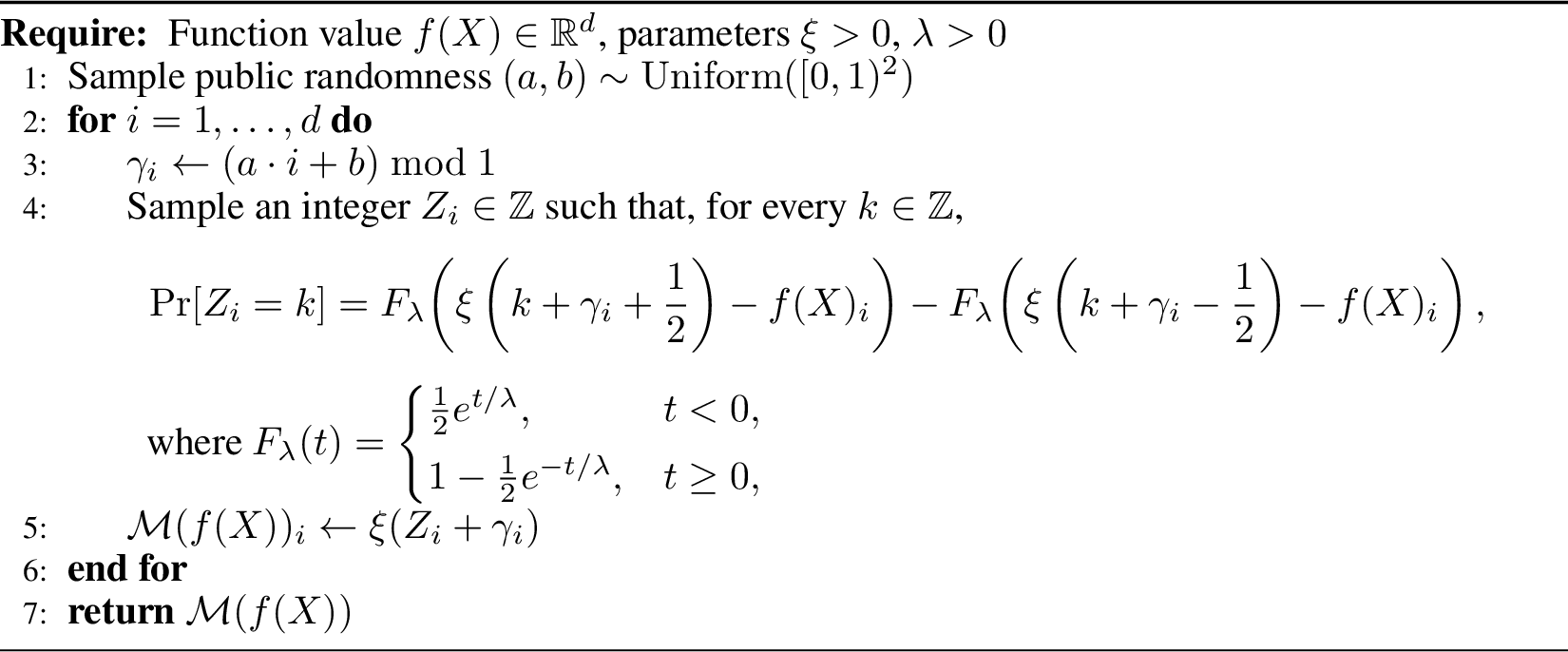
theoremMainUpperBound Suppose \(f:\mathbb{X}^*\rightarrow\mathbb{R}^d\) has sensitivity \(\Delta_1(f)\). For every \(\varepsilon > 0\), \(\beta\in (0,1)\), and \[\alpha > \frac{2\Delta_1(f)\log(d/\beta)}{\varepsilon},\] there exists a random variable \(U\) and mechanisms \(\mathcal{M}_U: \mathbb{X}^* \rightarrow\mathbb{R}^d\), defined by post-processing the Laplace mechanism on \(f(X)\), that are \(\varepsilon\)-differentially private for every fixed value of \(U\). Moreover, \(\mathcal{M}_U(f(X))\) is an \((\alpha,\beta)\)-accurate approximation of \(f(X)\), and its expected private randomness complexity satisfies \[\mathbb{E}_U\!\big[H(\mathcal{M}_U(f(X)))\big] = O\!\left( \frac{d\,\Delta_1(f)}{\alpha \varepsilon} \log\!\left(\frac{\alpha \varepsilon}{\Delta_1(f)}\right) \right).\]
Compared with Corollary [cor:csv-general-alpha], our bound removes the additive \(\log(d)\) term and improves the leading term by a factor of \(\log(d)\). For error tolerance \(\alpha = \omega(d \Delta_1(f) \log(d) / \varepsilon)\), the private randomness complexity becomes \(\mathbb{E}_U\!\big[H(\mathcal{M}_U(f(X)))\big] = o(1)\) independent of \(X\). That is, the mechanism requires only a negligible amount of fresh, private randomness to run. For error \(\alpha = \Theta(\Delta_1(f) \log(d/\beta)/\varepsilon)\), matching the \(\ell_\infty\)-error of the standard Laplace mechanism, the private randomness complexity is \(\mathbb{E}_U\!\big[H(\mathcal{M}_U(f(X)))\big] = O(d \log\log(d) / \log d)\) which is \(o(d)\). The mechanism’s public randomness \(U\) can be sampled using \(O(\log(d))\) random bits with high probability, matching the lower bound 5 on total randomness. We prove Theorem [thm:main95dithered95laplace], together with a bound on public randomness complexity, in the following lemma.
lemmamainTheoremDetailed Let \(f:\mathbb{X}^*\to\mathbb{R}^d\) have \(\ell_1\)-sensitivity \(\Delta_1(f)\). Consider the dithered Laplace mechanism \(\mathcal{M}\) defined in Algorithm 7 with parameters \(\xi>0\), \(\lambda>0\), and public randomness \(U=(a,b)\). Fix \(\beta\in(0,1)\). The mechanism satisfies:
Pure differential privacy: For every choice of \(\varepsilon>0\), if \(\lambda = \Delta_1(f)/\varepsilon\), then \(\mathcal{M}\) is \(\varepsilon\)-differentially private and \((\xi,\beta)\)-accurate with \[\xi = 2\,\Delta_1(f) \log(d/\beta)/\varepsilon.\]
Private randomness complexity: The mechanism has expected private entropy \[\mathbb{E}_U\!\big[H(\mathcal{M}_U(f(X)))\big]\;=\;O\!\left( \frac{d\,\lambda}{\xi}\, \log\!\frac{\xi}{\lambda} \right).\]
Public randomness complexity: If relaxed to output a special value \(\bot\) with probability at most \(\beta\), the mechanism can be implemented using \(O(\log(d/\beta))\) bits of public randomness.
Distributional properties: If relaxed to use an unbounded number of public random bits, the mechanism can be implemented such that it uses \(O(\log(d/\beta))\) public random bits with probability \(1-\beta\) and so that
it is unbiased, \(\mathbb{E}[\mathcal{M}(f(X))]=f(X)\), and
its coordinates are pairwise independent, \(\text{Cov}(\mathcal{M}(f(X))_i,\mathcal{M}(f(X))_j)=0\) for all \(i\ne j\).
Proof. We split the proof in five parts, covering privacy, error, private randomness complexity, public randomness complexity, and distributional properties, respectively.
Privacy. Conceptually the mechanism ensures \(\varepsilon\)-differential privacy by adding independent Laplace noise \(y \sim \text{Laplace}(\Delta_1(f)/\varepsilon)^d\) to the value \(f(X)\). The \(\ell_1\) sensitivity of \(f\) is \(\Delta_1(f)\), so Laplace noise with scale \(\lambda = \Delta_1(f) / \varepsilon\) ensures the required privacy guarantee for \(f(X) + y\). The subsequent rounding step maps the noisy result to the nearest point on an \(\xi\)-spaced grid shifted by the public offsets \(\xi\,\gamma_i\) with \(\gamma_i=(a i + b)\bmod 1\) and \((a,b)\sim\mathrm{Uniform}([0,1)^2)\). The public randomness \((a,b)\) is independent of the data, so post-processing preserves privacy for every fixed choice of \((a,b)\).
Error bound. As for the error incurred by the mechanism we note that \[\| \mathcal{M}(f(X)) - f(X) \|_\infty \leq \|y\|_\infty + \xi / 2,\] since the error in each coordinate is bounded by the sum of the perturbation given by \(y\) and the rounding to the nearest grid point which changes the value by at most \(\xi/2\). By a union bound over the coordinates, the probability that the noise exceeds \(\xi / 2\) is: \[\Pr[ \|y\|_\infty > \xi / 2 ] \leq d\, \exp\left( - \frac{\xi / 2}{\lambda} \right),\] which is less than \(\beta\) when \(\xi \geq 2\lambda \log(d/\beta)\). Thus, with probability at least \(1-\beta\) the total error is bounded by \(\xi\). Substituting \(\lambda = \Delta_1(f)/\epsilon\) completes the computation.
Private randomness complexity. Fix an arbitrary shift vector \(\gamma\in\mathbb{R}^d\) and condition on \(\gamma\) throughout this part; we only use its distribution at the end. For a given input \(z=f(X)\), define the (deterministic) baseline output \[\mathcal{M}_{\gamma,0}(z)\;:=\;\xi\cdot\Big(\Big\lfloor\frac{z}{\xi}-\gamma+\tfrac{1}{2}\Big\rfloor+\gamma\Big),\] obtained by setting the noise to zero. Let \(Y=(Y_1,\ldots,Y_d)\sim\mathrm{Laplace}(\lambda)^d\). The private entropy for this input and shift is \(H(\mathcal{M}_{\gamma,Y}(z))\), where \(\gamma\) is the public randomness. Since the coordinates of \(Y\) are independent and rounding is coordinate-wise, \(\mathcal{M}_{\gamma,Y}(z)\) is a deterministic function of independent integer “step counters” \(K_i\in\mathbb{Z}\) defined by \(\mathcal{M}_{\gamma,Y}(z)_i\;=\;\mathcal{M}_{\gamma,0}(z)_i\;+\;K_i\,\xi\). Hence \[\label{eq:entropy-sum} H(\mathcal{M}_{\gamma,Y}(z))\;\le H(K_1,\ldots,K_d\mid\gamma,z) \;=\;\sum_{i=1}^d H(K_i\mid\gamma,z),\tag{11}\] where the last equality uses independence of \(Y\). For \(i\in[d]\) let \(\tau_i=\tau_i(\gamma,z)\in[0,\xi/2]\) be the distance from \(z_i\) to the nearest boundary of the randomly shifted grid on the \(i\)th coordinate. That is, \[\tau_i:=\min_{k\in\mathbb{Z}}\{|z_i-\xi(k + \gamma_i + 1/2)|\}.\] For \(p_{0,i}(\gamma,z) :=\;1-e^{-\tau_i/\lambda}\) we have the following lower bound on the probability of \(K_i=0\): \[\Pr[\,K_i=0\mid\gamma,z\,]\;\geq \Pr[\,|Y_i|<\tau_i\,]\;=\;p_{0,i}(\gamma,z).\] For \(k\ge1\), crossing \(k\) grid boundaries requires \(|Y_i|\ge \tau_i+(k-1)\xi\), so the one-sided tail satisfies \[\Pr[\,|K_i|\ge k\mid\gamma,z\,]\;\le e^{-(\tau_i+(k-1)\xi)/\lambda} \;=\;e^{-\tau_i/\lambda}\,q^{\,k-1},\text{ where } q:=e^{-\xi/\lambda}.\] Thus \(|K_i|\) is stochastically dominated by a geometric distribution on \(\{1,2,\ldots\}\) with ratio \(q\), and the signed tail \(\{K_i=\pm k: k\ge1\}\) by a two-sided geometric (discrete Laplace) with the same ratio. Let \(h_2\) be the binary entropy function, and let \(H_\mathrm{geo}(q)\;:=\;-\log_2(1-q)\;-\frac{q}{1-q}\,\log_2 q\) be the entropy of a geometric\(\,(1-q)\) distribution on \(\{1,2,\ldots\}\). Encoding first the event \(\{K_i=0\}\) and then the signed magnitude gives \[\label{eq:Hi-bound} H(K_i\mid\gamma,z)\;\le h_2\big(p_{0,i}(\gamma,z)\big)\;+\;\big(1-p_{0,i}(\gamma,z)\big)\,\Big(\,1\;+\;H_\mathrm{geo}(q)\,\Big).\tag{12}\] Combining 12 over \(i\) with 11 yields a per-input, per-shift entropy bound.
Averaging over the shift. In our implementation the public shift is per-coordinate: \(\xi\,\gamma_i\) with \(\gamma_i=(a i + b)\bmod 1\) and \((a,b)\sim\mathrm{Uniform}([0,1)^2)\). For each fixed input \(z\) and coordinate \(i\), the marginal \(\gamma_i\sim\mathrm{Uniform}([0,1))\) is independent of \(Y_i\), so the remainder \((z_i-\xi\gamma_i)/\xi \text{ mod } 1\) is uniform on \([0,1)\). Consequently, the distance \(\tau_i(\gamma,z)\) from \(z_i\) to the nearest half-integer boundary is uniform on \([0,\xi/2]\). Hence \[\overline{p}_0\;:=\;\mathbb{E}_{\gamma}[\,p_{0,i}(\gamma,z)\,]\;=\;\mathbb{E}_{T\sim\mathrm{Uniform}([0,\xi/2])}[\,1-e^{-T/\lambda}\,] \;=\;1\;-\;\frac{2\lambda}{\xi}\Big(1-e^{-\xi/(2\lambda)}\Big),\] independent of \(i\) and \(z\). By concavity of \(h_2\) and linearity of expectation, \[\label{eq:per-coordinate-avg} \mathbb{E}_{\gamma}\big[\,H(K_i\mid\gamma,z)\,\big] \;\le h_2(\overline{p}_0)\;+\;(1-\overline{p}_0)\,\Big(\,1\;+\;H_\mathrm{geo}(q)\,\Big), \qquad q=e^{-\xi/\lambda}.\tag{13}\] Finally, \[\label{eq:entropy-final} \mathbb{E}_U\big[H(\mathcal{M}_U(z))\big] \;\le d\,\Big[\,h_2(\overline{p}_0)\;+\;(1-\overline{p}_0)\,\big(1+H_\mathrm{geo}(q)\big)\,\Big],\tag{14}\] with \(\overline{p}_0=1-\tfrac{2\lambda}{\xi}(1-e^{-\xi/(2\lambda)})\) and \(q=e^{-\xi/\lambda}\). Combining the above, we obtain an explicit asymptotic bound on the expected private entropy. Under the accuracy condition \(\xi \ge 2\lambda \log(d/\beta)\) established above (implying \(\xi/\lambda \gg 1\) in the regimes of interest), the geometric ratio \(q=e^{-\xi/\lambda}\) satisfies \(q\ll1\), and \(1-\overline{p}_0\;=\;\tfrac{2\lambda}{\xi}\big(1+O(e^{-\xi/(2\lambda)})\big)\). Using \(h_2(1-x)\le x\log_2(\tfrac{e}{x})\) and \(H_\mathrm{geo}(q)=\Theta(q\log\tfrac{1}{q})\) for small \(q\), inequality 14 yields \[\mathbb{E}_U[H(\mathcal{M}_U(z))]\;\le C\,d\cdot\frac{\lambda}{\xi}\,\log_2\frac{\xi}{\lambda}\] for some absolute constant \(C>0\). This establishes the claimed bound in part (b).
Public randomness complexity (for part (c)). Fix \(f(X)\) and the private noise \(y\). The output changes only when, for some coordinate \(i\in[d]\), the function \[\gamma_i \mapsto \frac{f(X)_i+y_i}{\xi}-\gamma_i+\tfrac12 \;=\;\frac{f(X)_i+y_i}{\xi}-\big((a\cdot i + b)\bmod 1\big)+\tfrac12\] crosses an integer. Equivalently, \((a,b)\in[0,1)^2\) lies in a set where \((a i + b)\bmod 1\) is within distance \(\eta\) of a (fixed) boundary point \(r_i\in[0,1)\) determined by \(f(X)_i\) and \(y_i\). For a precision parameter \(\eta\in(0,1)\), let \[\mathcal{B}_\eta\;:=\;\bigcup_{i=1}^d \Big\{(a,b)\in[0,1)^2\;:\;\mathop{\mathrm{dist}}\big((a i + b)\bmod 1,\;r_i\big)\le \eta\Big\}.\] Each set inside the union is the preimage (under the map \((a,b)\mapsto (a i+b)\bmod 1\)) of an interval of length \(2\eta\) in \([0,1)\), so its total area in \([0,1)^2\) is at most \(2\eta\). By the union bound, the probability mass of \(\mathcal{B}_\eta\) is at most \(2d\,\eta\). Now choose \(\eta:=\beta/(2d)\). Then \(\mu(\mathcal{B}_{\eta})\le \beta\). If we quantize \(a,b\) to \(m\) bits each with \[m=\left\lceil \log_2\frac{4d^2}{\beta}\right\rceil,\] then the rounded pair \((\tilde{a},\tilde{b})\) satisfies \[\mathop{\mathrm{dist}}\big((\tilde{a} i+\tilde{b})\bmod 1,(a i+b)\bmod 1\big) \le (i+1)2^{-m} \le \eta\] for every \(i\in[d]\). Thus, for every \((a,b)\notin\mathcal{B}_{\eta}\), the rounded pair \((\tilde{a},\tilde{b})\) determines the same output as \((a,b)\). Therefore, an implementation that outputs \(\bot\) whenever \((a,b)\in\mathcal{B}_{\eta}\) uses at most \(2m=O(\log(d/\beta))\) public bits and triggers \(\bot\) with probability at most \(\beta\). This proves part (c).
Public randomness complexity and distributional properties (for part (d)). If we allow unbounded public randomness, we can reveal the bits of \((a,b)\) incrementally until \((a,b)\notin\mathcal{B}_{\eta}\) is certified; with probability at least \(1-\beta\) this occurs by \(m=\lceil\log_2(4d^2/\beta)\rceil\) bits per parameter, so with probability \(1-\beta\) the public randomness used is \(O(\log(d/\beta))\) bits (and on the rare event we reveal more bits). Since \((a,b)\) are uniform on \([0,1)^2\), the induced shifts \(\gamma_i=(a i + b)\bmod 1\) satisfy: (i) for each \(i\), \(\gamma_i\sim\mathrm{Uniform}([0,1))\); and (ii) for \(i\neq j\), the pair \((\gamma_i,\gamma_j)\) is uniform on \([0,1)^2\). This pairwise independence property is a variant of classical constructions of pairwise independent hash functions [50], see Lemma 4 in Appendix 11 for a proof. Consequently, with the round-to-nearest construction, the per-coordinate quantization errors \(E_i=\mathcal{M}(f(X))_i-(f(X)_i+y_i)\) are pairwise independent and uniform on \([-\xi/2,\xi/2]\), independent of \((f(X),y)\), and in particular have mean zero. This proves part (d). ◻
11 Pairwise Independence of Affine Shifts↩︎
We now show the pairwise independence of the shift values \(\gamma\) in the dithered rounding scheme. The proof is analogous to Carter and Wegman’s classical proof of pairwise independence of random linear functions over finite fields [50]; we include it for completeness.
Lemma 4. Let \(a,b\sim\mathrm{Uniform}([0,1))\) be independent, and for each integer \(t\) define \(\gamma_t := (a t + b)\bmod 1 \in [0,1).\) Then for every \(t\) we have \(\gamma_t\sim\mathrm{Uniform}([0,1))\), and for distinct integers \(t\neq s\) the pair \((\gamma_t,\gamma_s)\) is uniform on \([0,1)^2\). In particular, \(\gamma_t\) and \(\gamma_s\) are (pairwise) independent.
Proof. We work on the unit interval \([0,1)\) with addition taken modulo \(1\). Write \(\{x\}\) for the fractional part of a real \(x\). Throughout, \(a,b\) are independent and uniform on \([0,1)\). Uniform marginal. Fix an integer \(t\). For any measurable set \(I\subseteq[0,1)\) and any fixed \(a\in[0,1)\), \[\Pr_b\!\big[\;\gamma_t\in I \bigm| a\;\big]\;=\;\Pr_b\!\big[\,\{ta+b\}\in I\,\big]\;=\;\Pr_b\!\big[\,b\in I-\{ta\}\,\big]\;=\;|I|,\] since \(b\mapsto \{b+c\}\) is a shift on the circle and preserves the total length of sets in \([0,1)\). Averaging over \(a\) gives \(\Pr[\gamma_t\in I]=|I|\), i.e., \(\gamma_t\sim{\rm Unif}[0,1)\). Pairwise independence. Let \(t\neq s\) be integers, and let \(I,J\subseteq[0,1)\) be measurable. We show \[\Pr\big[\;\gamma_t\in I,\;\gamma_s\in J\;\big]\;=\;|I|\,|J|.\] Condition on \(a\). For fixed \(a\), using \(b\) uniform and the shift argument as above, \[\begin{align} \Pr_b\!\big[\,\gamma_t\in I,\;\gamma_s\in J \bigm| a\,\big] &= \Pr_b\!\big[\mathop{\mathrm{frac}}(b+ta)\in I\quad\text{and}\quad\mathop{\mathrm{frac}}(b+sa)\in J\,\big] \\ &= \big|\, (I - \mathop{\mathrm{frac}}(ta)) \cap (J - \mathop{\mathrm{frac}}(sa)) \,\big|. \end{align}\] Set \(\delta:=\mathop{\mathrm{frac}}((t-s)a)\in[0,1)\) and note that \((I-\mathop{\mathrm{frac}}(ta))\cap (J-\mathop{\mathrm{frac}}(sa))=(J)\cap (I-\delta)\) up to a common shift, hence the length above equals \(\phi(\delta):=|\,J\cap (I-\delta)\,|\). Therefore \[\Pr\big[\;\gamma_t\in I,\;\gamma_s\in J\;\big]\;=\;\mathbb{E}_a\big[\,\phi(\{(t-s)a\})\,\big].\] We claim that \(\{(t-s)a\}\) is uniform on \([0,1)\) when \(a\) is uniform (for any nonzero integer \(t-s\)). Indeed, partition \([0,1)\) into \(|t-s|\) intervals of length \(1/|t-s|\); multiplication by \(|t-s|\) maps each interval linearly onto \([0,1)\), so for any measurable \(B\subseteq[0,1)\) the preimage \(\{a:\{(t-s)a\}\in B\}\) has size \(|B|\). Hence \(\{(t-s)a\}\sim{\rm Unif}[0,1)\). It remains to compute the average of \(\phi(\delta)\) over uniform \(\delta\). By averaging over all possible shifts and using that translating a set within [0,1) does not change its total length, \[\int_0^1 \phi(\delta)\,d\delta\;=\;\int_0^1 \Big( \int_0^1 \mathbf{1}_J(x)\,\mathbf{1}_I(x+\delta)\,dx \Big)\,d\delta \;=\;\int_0^1 \mathbf{1}_J(x)\,\Big( \int_0^1 \mathbf{1}_I(x+\delta)\,d\delta \Big)\,dx \;=\;|J|\cdot |I|.\] Therefore \(\mathbb{E}_a[\phi(\{(t-s)a\})]=|I|\,|J|\), and the desired equality follows. Since this holds for all measurable \(I,J\), the pair \((\gamma_t,\gamma_s)\) is uniform on \([0,1)^2\), and in particular \(\gamma_t\) and \(\gamma_s\) are independent. ◻