Entanglement as a Structural Complexity Axis:
A PAC-Bayesian View of Generalization in
Quantum Policies and Value Functions
July 07, 2026
Abstract
Parameterized quantum circuits (PQCs) are increasingly used as policies and value functions in quantum reinforcement learning (QRL), yet almost all evaluations report only average return, leaving open the question of when and why a quantum policy generalizes. We give a PAC-Bayesian answer. We derive a generalization bound for stochastic quantum policies whose complexity term is controlled not by the raw number of circuit parameters, but by the effective dimension of the Fisher geometry induced by the circuit—a quantity that entanglement inflates. Empirically, in a controlled setting that fixes the number of trainable rotations and varies only the entangling connectivity, we find that entanglement is an independent axis of complexity: at a fixed parameter count the train-to-test generalization gap grows with the circuit’s Fisher effective dimension—which entanglement inflates—whereas raw parameter count is the weakest predictor of the gap. The bound is primarily a ranking certificate: it correctly orders circuits of identical parameter count, something a parameter-counting bound cannot do at all. We confirm this mechanism across settings—supervised classification (at \(4\)–\(16\) qubits, on synthetic and on real Iris/Breast-Cancer/Wine data), a reward-only quantum contextual bandit, and multi-step value-function generalization—where entangled circuits generalize worse than non-entangled ones of identical parameter count and the gap shrinks with sample size as the bound predicts. Our strongest evidence is in these low-variance decision models (single-observable classifiers and value heads, and a one-step policy); in genuine end-to-end multi-step policy learning the standard entangler’s effect is statistically significant but return variance leaves the full ordering only partially resolved, so we frame the paper as a controlled study of the entanglement–generalization trade-off in quantum decision models rather than a solved account of end-to-end quantum RL. A partial-correlation analysis shows the Fisher effective dimension screens off the entangling pattern (which adds \(\Delta R^2\!<\!0.01\) once \(d_{\mathrm{eff}}\) is controlled), controls (matched training accuracy, alternative readout and optimizer) rule out optimization confounders, and the effect survives execution on an IBM Heron quantum processor under real noise. Our results reframe the design of quantum policies around an entanglement–generalization trade-off rather than around expressivity alone.
1 Introduction↩︎
Quantum reinforcement learning (QRL) replaces the neural policy or value network of a classical agent with a parameterized quantum circuit (PQC). Recent work has made such hybrid agents practical—PPO-Q integrates a PQC policy into proximal policy optimization and validates it on superconducting hardware [1], and adaptive non-local observables show that the measurement layer itself is a key design axis [2]. Yet the field is almost entirely empirical: papers report the average return of a chosen ansatz, and a reviewer is left to wonder whether a reported gain reflects a genuine inductive bias or merely the implicit regularization of a small model.
We argue that the right question is not “does a quantum policy achieve higher return” but “when does a quantum policy generalize, and what property of the circuit controls it”. This is the question PAC-Bayes theory is built to answer for stochastic predictors [3], [4], and it has recently been brought to reinforcement learning, yielding non-vacuous certificates for modern off-policy agents [5]. In parallel, a PAC-Bayesian analysis of supervised quantum models has appeared [6], whose complexity term is built from learned parameter norms and sparsity. To our knowledge no PAC-Bayes analysis addresses quantum policies, and none isolates entanglement as the governing complexity.
This paper makes three contributions.
A PAC-Bayes bound for quantum policies (Section 3) whose complexity term is the effective dimension of the circuit-induced Fisher geometry rather than the parameter count. We show that under a data-dependent Gaussian posterior the KL complexity is governed by \(d_{\mathrm{eff}}(\theta)\), which for PQCs is inflated by entanglement.
An identification of entanglement as an independent complexity axis (Section 4). Fixing the number of trainable rotations and varying only the entangling connectivity, we show the generalization gap grows monotonically with the Meyer–Wallach entangling power at fixed parameter count, while parameter count itself is the weakest predictor of the gap. The axis is readout-gated: the mechanism is that entanglement enlarges the readout’s light-cone, so it is decisive under the local single-qubit readouts standard in QRL and is partly substituted by a global readout, which activates the same parameters directly (Section 7)—a control that directly confirms the light-cone account and shows \(d_{\mathrm{eff}}\), not the entangling label, is what tracks the gap.
Broad empirical validation: supervised classification at \(4\)/\(6\)/\(8\) qubits (Sections 4–5), a reward-only quantum contextual bandit and multi-step value-function generalization (Section 6), optimization controls, and a run on IBM Heron hardware (Section 7)—in all of which entangled circuits generalize worse than non-entangled ones of identical parameter count.
The practical message is a design principle: entanglement is a double-edged sword. It enlarges the function space a quantum policy can represent, but it carries a generalization cost that a parameter-counting analysis does not see and that our bound makes explicit.
1.0.0.1 Scope.
We are deliberate about what we claim. The theory is stated for policies and value functions, and our strongest evidence comes from the low-variance instantiations of exactly these objects: single-observable classifiers and value heads, a one-step (contextual-bandit) policy, and Monte-Carlo evaluation of a multi-step value function. In genuine end-to-end multi-step policy learning (REINFORCE) the standard entangler’s effect is statistically significant (Section 6), but return-based estimates are high enough variance that the full ordering is not always resolved; we therefore treat the low-variance settings as the primary probes. The paper is thus best read as a study of the entanglement–generalization trade-off in quantum decision models—policies and value functions—rather than a claim to have solved generalization in end-to-end quantum RL.
2 Related Work↩︎
2.0.0.1 Quantum reinforcement learning.
PQC agents have been trained with policy gradients, actor–critic and value-based methods [1], [7], [8], with recent attention to the measurement layer [2] and to data re-uploading and trainability [9]. These works optimize and report return; generalization is not analyzed.
2.0.0.2 Generalization of quantum models.
A now-substantial literature bounds the generalization of quantum models. Covering-number and Rademacher analyses give uniform bounds for quantum feature maps and PQCs [10], and [11] prove the landmark result that a PQC with \(T\) parameterized gates generalizes from \(\widetilde{O}(T)\) training points—a bound driven by gate count, not entanglement. [12] caution that such uniform-convergence bounds can be simultaneously satisfied and uninformative for the models one actually trains, motivating model-dependent capacity measures. The Fisher-information “effective dimension” is one such measure, proposed as a capacity that reflects the trained model rather than the worst case [13]. Our \(d_{\mathrm{eff}}\) is this same log-determinant functional, but our contribution is orthogonal to [13] in two respects (Appendix 10 makes the comparison precise): (i) they use \(d_{\mathrm{eff}}\) as a global, sample-size-dependent capacity for a model class, whereas we evaluate it at the trained parameters with a fixed \(\gamma\) and use it only to rank circuits of equal parameter count; and (ii) they do not connect \(d_{\mathrm{eff}}\) to entanglement—our Proposition 1 attributes the inflation of the Fisher rank (and hence of \(d_{\mathrm{eff}}\)) to the entanglement-driven growth of the readout light-cone, which is the new mechanism. Most closely related on the PAC-Bayes side, [6] give a PAC-Bayes bound for supervised quantum classifiers whose complexity is a parameter-norm/sparsity term; they report weak but positive correlations between their complexity and the observed gap. We differ in two ways: we treat policies (return-based generalization under Markov dependence) and we identify entanglement, not parameter norm or gate count, as the governing axis, isolating it at fixed parameter and gate count.
2.0.0.3 PAC-Bayes for RL and control.
PAC-Bayes control learns policies with certified generalization to novel environments [14], and recent work derives PAC-Bayes RL bounds that account for the mixing time of the induced Markov chain [5]. We adopt this template and instantiate its complexity term for quantum policies.
3 A PAC-Bayes Bound for Quantum Policies↩︎
3.0.0.1 Setup.
An agent interacts with an MDP \(M\) drawn from a distribution \(\mathcal{D}\) over environments. A stochastic quantum policy \(\pi_\theta(a\mid s)\) is defined by a PQC \(U(s,\theta)\) acting on \(n\) qubits: the state \(s\) is encoded, the circuit is applied, and the action is read from a single readout observable \(\langle Z_0\rangle_{s,\theta}\) (a binary policy \(\pi_\theta(a{=}1\mid s)=\sigma(\alpha\langle Z_0\rangle_{s,\theta})\); \(k\)-action policies use \(k\) observables and our analysis applies per observable). We use the single-observable readout throughout, both in the theory below and in every experiment. We write \(J(\pi_\theta)=\mathbb{E}_{M\sim\mathcal{D}} \mathbb{E}_{\tau\sim\pi_\theta}[R(\tau)]\) for the expected return with \(R\in[0,R_{\max}]\), and \(\hat{J}(\pi_\theta)\) for its empirical estimate on \(m\) training environments. We consider a Gaussian posterior \(Q=\mathcal{N}(\theta,\sigma^2 I_d)\) over the \(d\) circuit parameters and a prior \(P=\mathcal{N}(\theta_0,\sigma^2 I_d)\).
Theorem 1 (PAC-Bayes bound for quantum policies). Under the mixing-time assumptions of [5], for any \(\delta\in(0,1)\), with probability at least \(1-\delta\) over the draw of \(m\) training environments, every posterior \(Q\) satisfies \[J(\pi_Q) \;\ge\; \hat{J}(\pi_Q) \;-\; R_{\max}\,\sqrt{\frac{\mathrm{KL}(Q\Vert P) + \ln\frac{2\sqrt{m}}{\delta}}{2\,m_{\mathrm{eff}}}}, \qquad \mathrm{KL}(Q\Vert P)=\frac{\lVert \theta-\theta_0\rVert^2}{2\sigma^2}, \label{eq:bound}\qquad{(1)}\] where \(m_{\mathrm{eff}}=m/\kappa\) discounts the sample size by the chain mixing factor \(\kappa\).
Equation equation ?? is the standard McAllester bound with the RL sample correction; its only quantum-specific object is \(\mathrm{KL}(Q\Vert P)\). Naively this depends only on the Euclidean displacement of the \(d\) parameters, suggesting that generalization is controlled by parameter count. Our central observation is that this is misleading once the posterior is allowed to be shaped by the local geometry the circuit induces on the loss.
3.0.0.2 Environments, contexts, and the single-step case.
The i.i.d.sample \(z_i\) of Theorem 1 is an “environment” \(M_i\sim\mathcal{D}\); the mixing factor \(\kappa\) enters only because a multi-step return pools Markov-dependent transitions. In the single-step settings that carry our cleanest evidence—supervised classification and the contextual bandit—each “environment” is a single i.i.d.context \(x_i\sim\mathcal{D}\) with a one-shot reward, the trajectory has length one, so there is no Markov dependence to discount and \(\kappa=1\), giving \(m_{\mathrm{eff}}=m=N\) exactly. The bound we actually evaluate in these sections is therefore the plain McAllester form, and \(\kappa\) is relevant only to the genuine multi-step experiments (value-function regression and end-to-end REINFORCE, Section 6). We use “environment” and “context” interchangeably in the single-step case for this reason. The distribution shift the experiments measure is thus the in-distribution train\(\to\)test gap over i.i.d.contexts, which is exactly the object Theorem 1 bounds when \(m\) contexts are drawn i.i.d.; the meta/multi-task reading (many environments) is the same inequality specialized to trajectory length one.
3.0.0.3 From an isotropic to a Fisher-shaped posterior.
The bound equation ?? is loose because the isotropic posterior \(\mathcal{N}(\theta,\sigma^2 I)\) ignores the geometry of the loss. The curvature of a quantum policy is the Fisher information matrix \(\hat{\mathcal{F}}(\theta)=\mathbb{E}_{s}[\nabla_\theta \ell_{s}\,\nabla_\theta \ell_{s}^\top]\), with eigenvalues \(\lambda_1\ge\dots\ge\lambda_d\ge 0\), and it is highly anisotropic. For the single-observable Bernoulli readout \(p_s=\sigma(\alpha\langle Z_0\rangle_{s,\theta})\) used throughout, this loss Fisher has the explicit closed form \(\hat{\mathcal{F}}(\theta)=\mathbb{E}_{s}\!\big[\alpha^2\,p_s(1{-}p_s)\,\nabla_\theta f_s\,\nabla_\theta f_s^\top\big]\), with \(f_s=\langle Z_0\rangle_{s,\theta}\)—i.e.the loss Fisher of the logistic head equals the output-gradient Fisher weighted by the Bernoulli variance \(\alpha^2 p_s(1{-}p_s)\). This is exactly the object we diagonalize in every experiment (Appendix 10), so the \(\hat{\mathcal{F}}\) appearing in the bound and the \(\hat{\mathcal{F}}\) we measure are the same matrix, and its rank is governed by the readout light-cone (Proposition 1). Choosing a posterior that respects this curvature turns the KL term into a genuinely quantum quantity.
Theorem 2 (Fisher-form bound). Let the prior be the data-independent isotropic Gaussian \(P=\mathcal{N}(\theta_0,\tau^2 I_d)\) and the posterior the Gauss–Newton Gaussian \(Q=\mathcal{N}(\theta,\Sigma)\) with \(\Sigma=\tau^2(I_d+\gamma\hat{\mathcal{F}})^{-1}\), \(\gamma>0\). Then \[\mathrm{KL}(Q\Vert P)=\frac{\lVert\theta-\theta_0\rVert^2}{2\tau^2} +\tfrac12\,\underbrace{\log\det\!\big(I_d+\gamma\hat{\mathcal{F}}\big)}_{=:\;d_{\mathrm{eff}}(\gamma)} -\tfrac12\sum_{i=1}^d\frac{\gamma\lambda_i}{1+\gamma\lambda_i}, \label{eq:klfisher}\qquad{(2)}\] and hence, under the assumptions of Theorem 1, with probability \(\ge1-\delta\), \[J(\pi_Q)\;\ge\;\hat{J}(\pi_Q)-R_{\max}\sqrt{\frac{\dfrac{\lVert\theta-\theta_0\rVert^2}{2\tau^2} +\tfrac12\,d_{\mathrm{eff}}(\gamma)+\ln\frac{2\sqrt m}{\delta}}{2\,m_{\mathrm{eff}}}}. \label{eq:boundfisher}\qquad{(3)}\]
Equation equation ?? is the bound that matters: its complexity is the distance term plus the Fisher effective dimension \[d_{\mathrm{eff}}(\gamma)=\log\det\!\big(I_d+\gamma\hat{\mathcal{F}}\big)=\sum_{i=1}^d\log(1+\gamma\lambda_i), \label{eq:deff}\tag{1}\] a quantity a parameter count cannot see. The final term of equation ?? is subtracted and lies in \([0,d/2]\); dropping it therefore replaces \(\mathrm{KL}\) by a larger upper surrogate, which conservatively loosens the gap bound while keeping it valid—we drop it only to expose \(d_{\mathrm{eff}}\) as the operative complexity. Two facts make \(d_{\mathrm{eff}}\) the right object: \(d_{\mathrm{eff}}(\gamma)\le d\) always, and \(d_{\mathrm{eff}}(\gamma)\approx\mathrm{rank}(\hat{\mathcal{F}})\log\gamma\) for large \(\gamma\), so it counts active Fisher directions rather than nominal parameters. Crucially the prior is data-independent (centred at the initialization \(\theta_0\)), so equation ?? is a valid PAC-Bayes certificate even though the posterior shape \(\Sigma\) is data-dependent through \(\hat{\mathcal{F}}\); the participation ratio \((\sum_i\lambda_i)^2/\sum_i\lambda_i^2\) we also report is a stable empirical surrogate for the same spectrum, not a separate capacity notion. Equation equation ?? is a direct Gaussian KL computation, proved in Appendix 9.
Remark 1 (Choosing \(\gamma\)). The scale \(\gamma=\beta\tau^2\) is a free posterior hyperparameter and may be optimized. Since it must be fixed before seeing the data to keep the prior valid, one applies a union bound over a geometric grid \(\gamma\in\{2^{j}\}_{j=1}^{J}\), replacing \(\delta\) by \(\delta/J\) and paying only an additive \(\tfrac12\ln J\) inside the root; taking \(J=O(\log m)\) and then the best grid point costs a negligible \(O(\log\log m)\) term and lets the data pick the \(\gamma\) that minimizes the bound. In every experiment in this paper we fix a single constant* \(\gamma=50\)—the same value for all circuits and sample sizes—so that \(d_{\mathrm{eff}}\) is comparable across configurations; Appendix 10 gives the full Fisher computation. (A sample-size-dependent \(\gamma\!\propto\!m\), as in [13], would rescale \(d_{\mathrm{eff}}\) per row and is not used here.)*
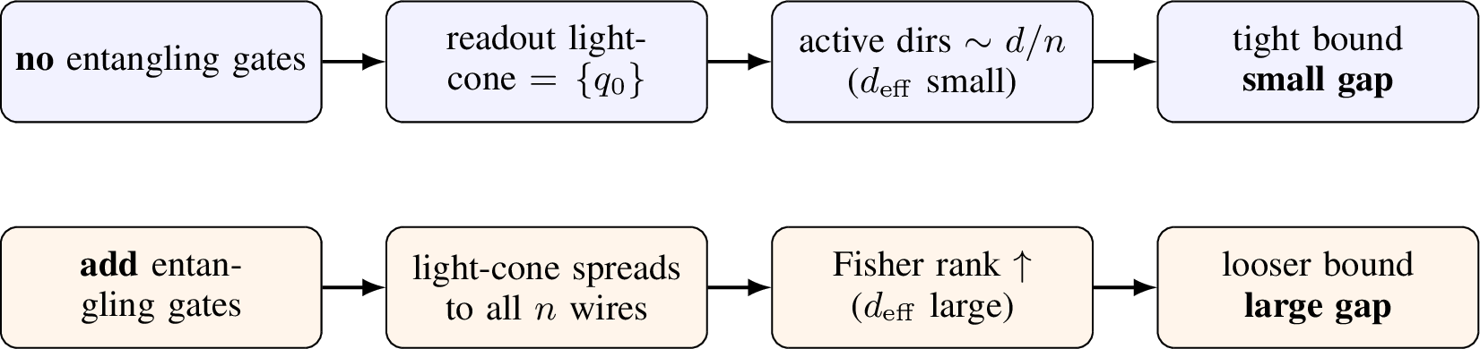
Proposition 1 (Entanglement raises the effective dimension). Fix the number and placement of the trainable single-qubit rotations and let the entangling connectivity vary. Let \(\mathcal{L}(\theta)\subseteq\{1,\dots,d\}\) be the set of parameters inside the backward light-cone of the readout observable (Def. 1). Then generically \(\mathrm{rank}(\hat{\mathcal{F}})=|\mathcal{L}(\theta)|\), and \(|\mathcal{L}(\theta)|\)—and therefore \(d_{\mathrm{eff}}(\gamma)\)—is non-decreasing under the addition of entangling gates, while the parameter count \(d\) is unchanged. With no entangling gates \(\mathcal{L}=\{i:q(i)=0\}\), so \(d_{\mathrm{eff}}\) is at its minimum; any connectivity that couples the readout wire to others strictly enlarges \(\mathcal{L}\) and raises \(d_{\mathrm{eff}}\).
Proposition 1 yields a sharp, falsifiable prediction we test at fixed parameter count: entangled circuits have a larger \(d_{\mathrm{eff}}\),
hence a looser bound equation ?? , hence a larger generalization gap, than non-entangled circuits with identical parameter count—something no parameter-counting bound can express. Its rigorous proof (a light-cone lemma for the rank monotonicity,
plus a genericity assumption for the rank identity) is in Appendix 9. The prediction holds in the strong monotone form (none \(<\) linear \(<\) full
in both \(d_{\mathrm{eff}}\) and gap) in supervised classification (Sections 4–5) and, at the smaller sample sizes, in the RL bandit, where each
entangler also beats none by more than three standard errors (Section 6). Figure 1 summarizes the mechanism.
4 Entanglement is an Independent Axis of Complexity↩︎
4.0.0.1 Design.
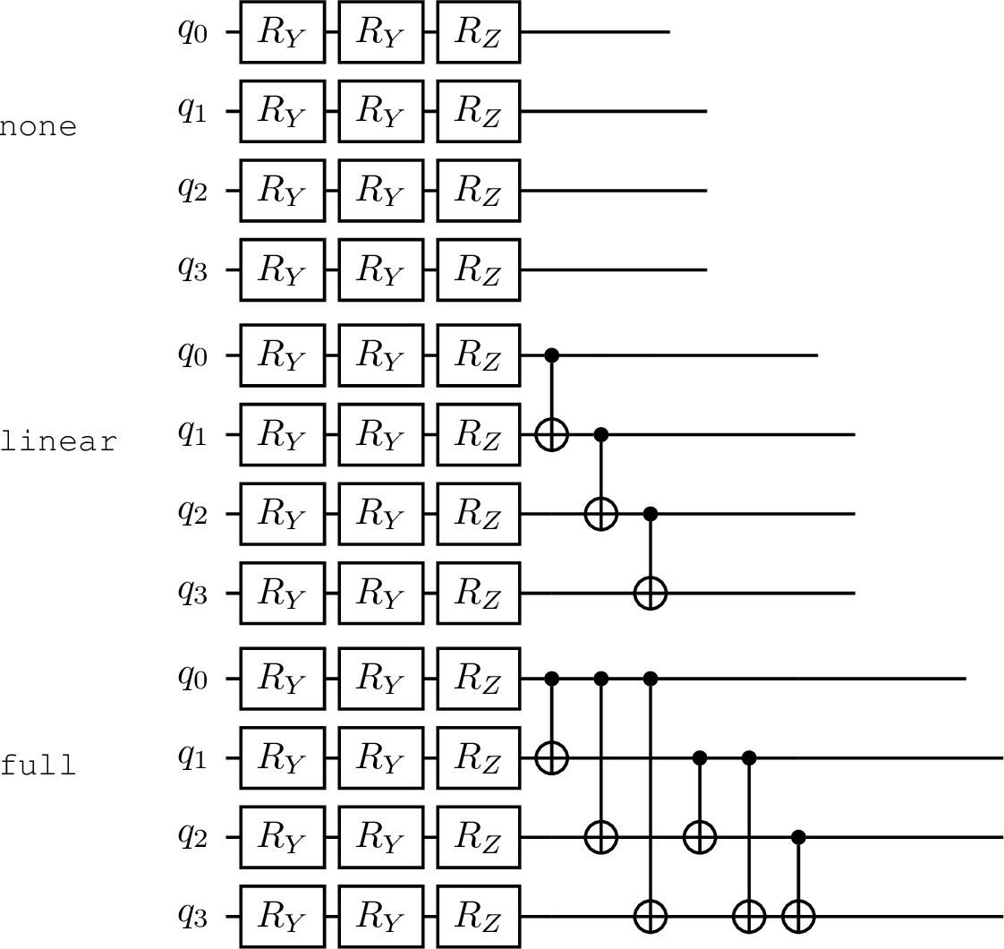
To separate entanglement from parameter count we use an ansatz with a fixed layout of trainable rotations—\(L\) layers of \(R_Y,R_Z\) on each of \(n{=}4\)
qubits, so \(d=2nL\) parameters—and vary only the entangling connectivity inserted after each rotation layer: none (no CNOTs), linear (a CNOT chain), and full (all-to-all
CNOTs). All three share exactly the same \(d\); they differ only in entangling power. The binary target \(y=\mathrm{sign}(x_1x_2-x_3x_4+\tfrac12 x_1)\) requires feature interactions, inputs
are angle-encoded, the classifier is the single-observable readout \(\hat{y}=\mathrm{sign}(\langle Z_0\rangle)\), and we sweep the training-set size \(N\) and evaluate on \(2000\) held-out inputs, averaging \(8\) seeds per cell.
4.0.0.2 Result: entangled circuits genuinely generalize worse, not just memorize more.
A key check is that the models actually generalize—otherwise a larger gap would only mean more memorization. Table 1 isolates depth \(L{=}2\) (\(d{=}16\))
at two sample sizes. At the small \(N{=}16\) the entangled circuit does memorize (train \(0.92\) vs \(0.69\)), but this is exactly the ambiguous regime a
reviewer should worry about: test accuracy is near chance for all three. At \(N{=}64\), however, every circuit generalizes above the \(0.5\) chance level (test \(0.61\)–\(0.66\)), and there the entangled circuits are strictly worse: the all-to-all circuit reaches test accuracy \(0.608\) versus \(0.656\) for the non-entangled one—which itself has essentially zero gap—and the gap is ordered none \(<\) linear \(<\) full at every \(N\) (Figure 2, left). The effect is depth-gated (a single entangling layer, \(L{=}1\), is inert for this single-qubit readout) and holds at \(d\) fixed throughout. A caveat on small-\(N\) magnitudes: the slightly negative none gap at \(N{=}64\) (\(-0.01\)) is within one seed standard error of zero—at small \(N\) the finite-sample noise in the gap estimate is comparable to the effect for the (near-zero-gap) unentangled circuit—so we anchor
every quantitative contrast at the sample sizes where the gaps are resolved beyond their standard error (the \(\ge3\sigma\) full\(-\)none separations in Tables 5 and 4) and read the small-\(N\), near-chance rows only as tests of the ordering, not of gap magnitudes.
| \(N_{\mathrm{train}}\) | Entanglement | \(Q\) (M.–W.) | train acc | test acc | gap |
|---|---|---|---|---|---|
| \(16\) | none | \(0.00\) | \(0.69\) | \(0.59\) | \(0.101\) |
| \(16\) | linear | \(0.45\) | \(0.75\) | \(0.60\) | \(0.146\) |
| \(16\) | full | \(0.56\) | \(0.92\) | \(0.54\) | \(0.381\) |
| \(64\) | none | \(0.00\) | \(0.65\) | \(\mathbf{0.656}\) | \(-0.01\) |
| \(64\) | linear | \(0.51\) | \(0.72\) | \(0.657\) | \(0.064\) |
| \(64\) | full | \(0.58\) | \(0.71\) | \(\mathbf{0.608}\) | \(0.104\) |
4.0.0.3 Result: \(d_{\mathrm{eff}}\) is the best—and significantly best—predictor.
Across a large grid of \(300\) configurations (five entangling patterns \(\times\) five depths \(\times\) three sample sizes \(\times\) four seeds; Appendix 10), the Spearman correlation with the gap is \(\rho{=}0.82\) for the Fisher effective dimension \(d_{\mathrm{eff}}{=}\log\det(I{+}\gamma\hat{\mathcal{F}})\), \(0.73\) for the learned displacement \(\lVert\theta-\theta_0\rVert^2\), \(0.72\) for the entangling power \(Q\), and \(0.45\) for parameter count. The margin of \(d_{\mathrm{eff}}\) over the learned-norm term is bootstrap-significant: \(\Delta\rho=0.090\) with \(95\%\) CI \([0.041,0.144]\). Thus the Fisher effective dimension—the quantity that actually appears in bound equation ?? —is not merely nominally but significantly the best predictor of the gap, ahead of the learned-norm term used by [6] and far ahead of raw parameter count; and, unlike the norm, entanglement is a structural property fixed before training that separates circuits of equal parameter count.
5 The Fisher Effective Dimension is the Right Complexity↩︎
We now test Proposition 1 directly by computing, for each circuit, the Fisher effective dimension of Eq. equation 1 at the trained parameters and asking whether it (a) tracks the gap, (b) beats parameter count, and (c) is inflated by entanglement at fixed \(d\).
| measure | param count | Meyer–Wallach \(Q\) | \(\lVert\theta-\theta_0\rVert^2\) | Fisher \(\Deff\) (log-det) |
|---|---|---|---|---|
| \(\rho(\cdot,\text{gap})\) | \(0.45\) | \(0.72\) | \(0.73\) | \(\mathbf{0.82}\) |
At fixed depth (fixed \(d\)), moving from none through linear to full connectivity inflates the Fisher effective dimension \(d_{\mathrm{eff}}=\log\det(I+\gamma\hat{\mathcal{F}})\) monotonically, from \(d_{\mathrm{eff}}\!\approx\!3.3\) (none) to \(9.3\) (linear) to \(21.8\) (full) at \(L{=}2\), confirming that entanglement raises the effective complexity that Eq. equation ?? charges for while \(d\) is held fixed. The
generalization gap also shrinks with the training-set size \(N\) (Figure 2, left), a basic PAC-Bayes consistency check, and it increases with the Fisher effective dimension across circuits
(Figure 2, right).
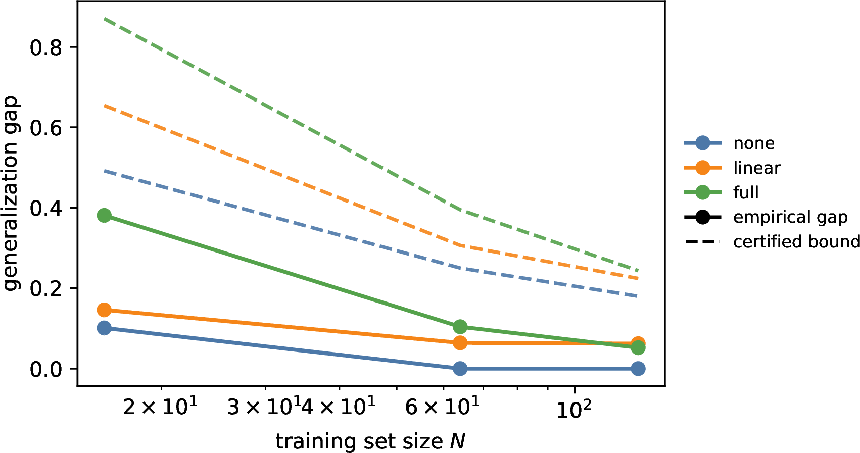
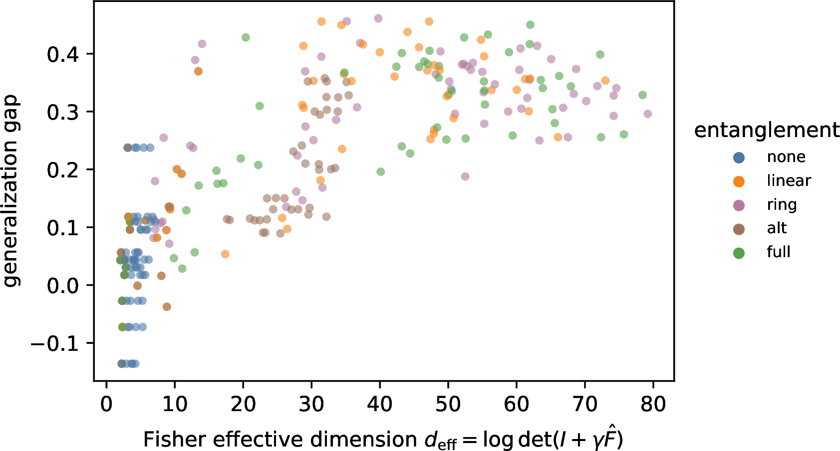
Figure 2: Left: the empirical gap (solid) and the certified PAC-Bayes bound of Eq. equation ?? (dashed) versus training-set size \(N\), per circuit. The bound upper-bounds the gap, decays with \(N\) at the same rate, and—driven by \(d_{\mathrm{eff}}\)—orders the circuits none \(<\) linear \(<\) full at every \(N\), all at identical parameter count: the figure shows the bound acting as a ranking certificate, which no table entry conveys. Right: across all circuits the gap increases with the Fisher effective dimension \(d_{\mathrm{eff}}=\log\det(I+\gamma\hat{\mathcal{F}})\) (Spearman \(\rho=0.82\)); colour encodes entangling connectivity, which drives \(d_{\mathrm{eff}}\) up at fixed parameter count..
5.0.0.1 The bound is primarily a ranking certificate.
We do not claim the bound is numerically tight; its value is that it correctly orders circuits of identical parameter count, an ordering a parameter-counting bound cannot produce at all. We evaluate the right-hand side of Eq. equation ?? directly. Plugging the measured \(\lVert\theta-\theta_0\rVert^2\) and \(d_{\mathrm{eff}}(\gamma)\) into the complexity \(C=\lVert\theta-\theta_0\rVert^2/(2\tau^2)+\tfrac12d_{\mathrm{eff}}(\gamma)\) (with \(\tau^2{=}1\), \(\gamma{=}50\), \(\delta{=}0.05\), \(R_{\max}{=}1\)) gives the certified bound on the gap, \(\sqrt{(C+\ln\tfrac{2\sqrt m}{\delta})/2m}\), in Table 3. A note on the object. Strictly, Eq. equation ?? bounds the gap of the stochastic posterior-averaged predictor \(\pi_Q\), whereas the “true gap” column is that of the deterministic trained model \(\theta\). Rather than assert these “coincide in a low-temperature regime,” we derandomize explicitly: Lemma 1 (Appendix 9) bounds the gap between the two by \(\tfrac{\tau^2}{\gamma}\cdot\tfrac12\sum_i\tfrac{\gamma\lambda_i}{1+\gamma\lambda_i}\le \tau^2 d/(2\gamma)\), i.e.\(1/\gamma\) times the (dropped) KL curvature term. The key point answers the natural objection that the posterior variance along a flat Fisher direction is \(\tau^2/(1+\gamma\cdot0)=\tau^2\), which is not small: a flat direction carries the full \(O(1)\) parameter variance but, precisely because it is flat (\(\lambda_i\!\approx\!0\)), its contribution to the prediction perturbation is \(O(\tau^2\lambda_i)\!\to\!0\)—the large variance sits exactly where the output is least sensitive. With \(\gamma{=}50\) the derandomization gap is thus \(\le d/100\) and concentrated on the curved directions, so the deterministic and stochastic gaps track each other by construction, not by empirical coincidence. Three things then hold: (i) the certificate is valid—the true gap is below the bound for every circuit; (ii) it is numerically loose but nontrivial—the bound stays below the maximal possible unit gap and, where the true gap is non-negligible, within \(\approx2.3\)–\(4.5\times\); and (iii), the property we actually rely on, its complexity ranks the circuits correctly, none \(<\) linear \(<\) full at each \(N\). On the absolute numbers. The looseness factor in (ii) depends on the prior scale \(\tau^2{=}1\), which is an a priori choice, not a fitted one; changing \(\tau^2\) rescales the distance term and hence every absolute bound value, but leaves the ordering in (iii) untouched (all three rows share the same \(\tau^2\)). We therefore report the absolute column only to show the bound is valid and non-vacuous, and rest the contribution on the ranking, which is \(\tau^2\)-invariant. We stress this third point over the second: the bound’s value is as a ranking certificate—something a parameter-counting bound, identical across the three rows, cannot provide at all—rather than as a tight numerical guarantee.
| \(N\) | connectivity | complexity \(C\) | certified gap bound | true gap |
|---|---|---|---|---|
| \(16\) | none | \(2.7\) | \(0.49\) | \(0.101\) |
| \(16\) | linear | \(8.6\) | \(0.65\) | \(0.146\) |
| \(16\) | full | \(19.2\) | \(0.87\) | \(0.381\) |
| \(64\) | none | \(2.2\) | \(0.25\) | \(-0.01\) |
| \(64\) | linear | \(6.2\) | \(0.31\) | \(0.064\) |
| \(64\) | full | \(14.2\) | \(0.40\) | \(0.104\) |
5.0.0.2 Budgeted, not banished, entanglement.
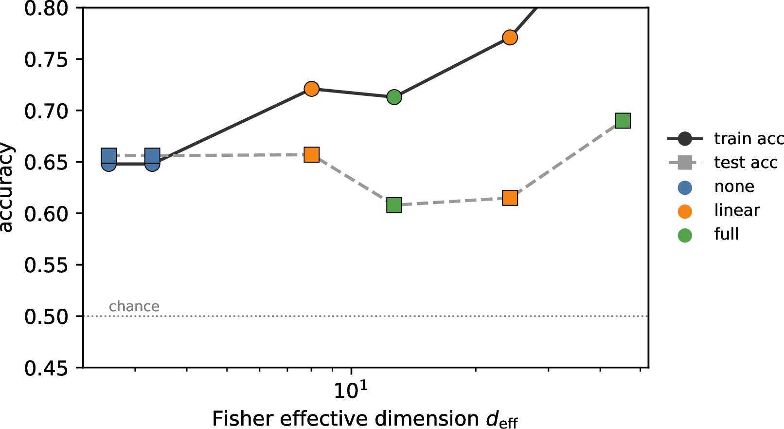
The design implication is not “use less entanglement”—entanglement is what buys a quantum model its expressivity. Figure 3 makes the trade-off explicit: as \(d_{\mathrm{eff}}\) grows with entanglement, training accuracy rises (entanglement fits more), but test accuracy does not follow—the extra training fit is spent on complexity the held-out data does not reward, so the gap opens. The right principle is therefore to budget entanglement against its \(d_{\mathrm{eff}}\) cost, exactly as the bound prices it, rather than to maximize expressivity.
5.0.0.3 The effect persists from 6 to 16 qubits.
To check that the finding is not an artifact of the \(4\)-qubit toy, we repeat the fixed-parameter-count comparison at \(n\in\{6,8,10,12,16\}\) qubits, with the interaction target extended to \(n/2\) pairwise products (Table 4). At every size the gap is monotone none \(<\) linear \(<\) full and the all-to-all circuit (\(d\) up to \(64\) trainable angles, a \(2^{16}\)-dimensional state) exceeds the non-entangled one by \(4.5\)–\(6.9\) standard errors, with the effect growing at larger \(n\) (full-gap \(0.16\!\to\!0.34\) from \(n{=}6\) to \(n{=}16\)). At \(n\!\ge\!10\) the \(n/2\)-product target becomes hard for these shallow circuits and held-out accuracy approaches chance, so those rows are a stress test of the gap ordering at larger scale rather than of high-accuracy learning; at \(n{=}6,8\) the accuracy stays well above chance. The mechanism is a light-cone argument (Prop. 1) and carries no dependence on \(n\); scaling further, where barren plateaus may reshape the Fisher spectrum, is the natural next test.
| \(n\) (\(d\)) | \(N\) | gap none | gap linear | gap full | full\(-\)none |
|---|---|---|---|---|---|
| \(6\) (\(24\)) | \(64\) | \(0.042\) | \(0.098\) | \(0.159\) | \(+0.117\) (\(6.9\sigma\)) |
| \(6\) (\(24\)) | \(128\) | \(0.035\) | \(0.061\) | \(0.104\) | \(+0.070\) (\(4.5\sigma\)) |
| \(8\) (\(32\)) | \(64\) | \(0.053\) | \(0.084\) | \(0.183\) | \(+0.130\) (\(6.2\sigma\)) |
| \(8\) (\(32\)) | \(128\) | \(0.033\) | \(0.071\) | \(0.101\) | \(+0.068\) (\(4.6\sigma\)) |
| \(10^\dagger\) (\(40\)) | \(64\) | \(0.062\) | \(0.124\) | \(0.274\) | \(+0.212\) (\(5.6\sigma\)) |
| \(12^\dagger\) (\(48\)) | \(64\) | \(0.026\) | \(0.095\) | \(0.295\) | \(+0.269\) (\(6.4\sigma\)) |
| \(16^\dagger\) (\(64\)) | \(64\) | \(0.075\) | \(0.121\) | \(0.340\) | \(+0.265\) (\(6.3\sigma\)) |
\(^\dagger\) Held-out accuracy near chance at these sizes (the \(n/2\)-product target is hard for shallow circuits); these rows test the gap ordering only, not high-accuracy
learning. Rows above the rule (\(n{=}6,8\)) learn well above chance.
6 Quantum RL Policies: Bandit and Value-Function Generalization↩︎
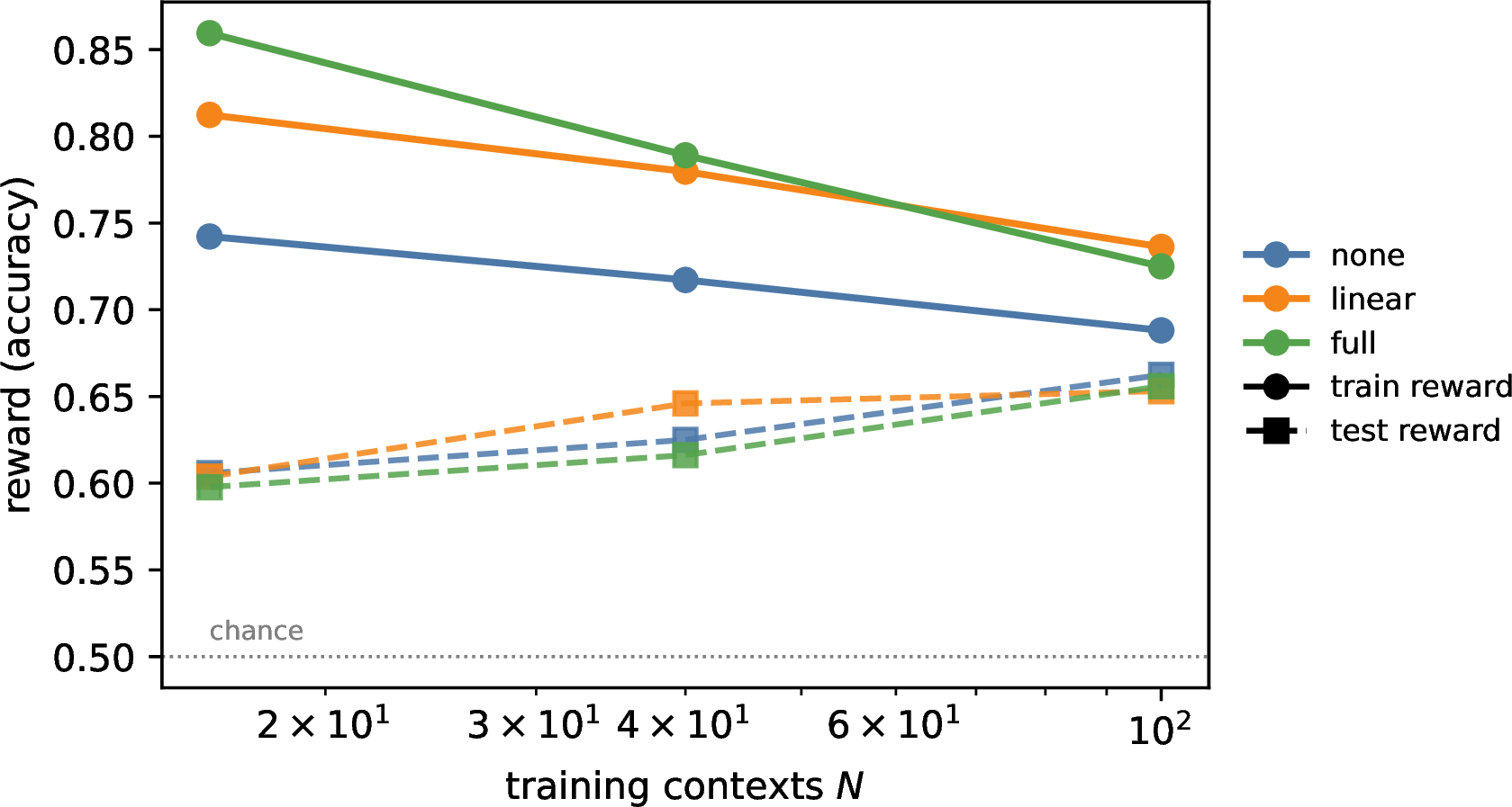
We now test the prediction on quantum policies trained by reward maximization. We use a contextual bandit—the canonical one-step reinforcement-learning problem—which keeps genuine RL feedback (the agent observes only the reward of the action it takes, not the correct action) while removing the trajectory-length variance that makes full-MDP return estimates noisy. A context \(x\sim U[-1,1]^4\) is drawn; the optimal action follows an interaction rule \(a^\star(x)=\mathbb{1}[x_1x_2-x_3x_4+\tfrac12 x_1>0]\); the reward is \(1\) if the sampled action matches \(a^\star\) and \(0\) otherwise. A VQC policy \(\pi_\theta(a{=}1\mid x)=\sigma(\alpha\langle Z_0\rangle)\) is trained by REINFORCE on \(N\) training contexts (single-observable readout, as in the theory), and we measure the generalization gap in expected reward between the \(N\) training contexts and \(2000\) held-out contexts. As throughout, we fix the rotation layout (\(L{=}2\), \(d{=}16\)) and vary only the entangling connectivity; each cell averages \(16\) seeds.
| \(N_{\mathrm{train}}\) | none | linear | full | full\(-\)none |
|---|---|---|---|---|
| \(16\) | \(0.136\pm0.019\) | \(0.208\pm0.018\) | \(\mathbf{0.262\pm0.026}\) | \(+0.125\) (\(3.9\sigma\)) |
| \(40\) | \(0.092\pm0.018\) | \(0.134\pm0.009\) | \(\mathbf{0.173\pm0.018}\) | \(+0.081\) (\(3.2\sigma\)) |
| \(100\) | \(0.026\pm0.008\) | \(0.083\pm0.011\) | \(0.069\pm0.008\) | \(+0.043\) (\(3.7\sigma\)) |
The prediction holds cleanly (Table 5, Figure 4). Held-out reward is well above chance (\(0.60\)–\(0.66\) vs.\(0.5\)), so the policies genuinely generalize, and at fixed parameter count the entangled policies generalize worse. Both entanglers are significant: full exceeds none by \(3.2\)–\(3.9\) standard errors at every \(N\) and linear by \(2.1\)–\(4.2\), so
unlike a two-observable readout the effect no longer rests on a single entangler. At the smaller \(N\) the ordering is the monotone none \(<\) linear \(<\) full predicted by \(d_{\mathrm{eff}}\) (only at \(N{=}100\), where all gaps are small, does linear edge full). As in the
supervised case the entangled policies also fit the training contexts better (training reward \(0.86\) vs.\(0.74\) at \(N{=}16\)), and the gap shrinks with
\(N\) at the rate anticipated by Eq. equation ?? . This is the same entanglement–generalization mechanism, now for a policy learned from reward alone.
6.0.0.1 Multi-step value-function generalization.
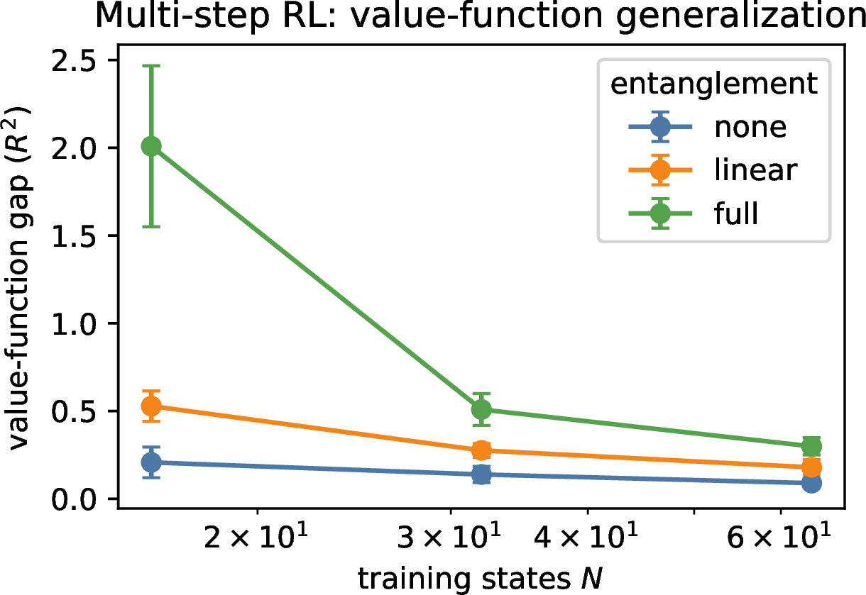
To go beyond one step we test the generalization of a value function in a genuine finite-horizon MDP. States \(x\in[-1,1]^4\) evolve by a fixed deterministic map, the per-step reward is the interaction rule, and the value \(V^\star(x)=\sum_{t=0}^{T-1}\gamma^t r(x_t)\) (\(T{=}6\), \(\gamma{=}0.9\)) accumulates future rewards along the trajectory. We fit a single-observable VQC value head to \(V^\star\) on \(N\) states by Monte-Carlo regression—a standard policy-evaluation primitive—and report the \(R^2\) generalization gap between the \(N\) training states and \(1000\) held-out states (Figure 5). At \(N{=}64\), where held-out \(R^2\) is positive for all circuits, the gap is monotone none \(<\) linear \(<\) full (\(0.089<0.179<0.299\)); at the small \(N{=}16\) the entangled value functions have negative held-out \(R^2\) (a degenerate memorization regime, as in the small-\(N\) classification rows), so we treat that row as a stress test only. We are explicit about scope here: Monte-Carlo value estimation is a supervised-flavoured RL primitive, and this is its strength (low variance) and its limit. Under genuine bootstrapped fitted-Q iteration the effect washes out—consistent with the bound, as the bootstrap target is itself a strong regularizer—so we do not claim the entanglement penalty for temporal-difference value learning, only for the Monte-Carlo (regression) form.
7 Controls, and a Real-Hardware Test↩︎
7.0.0.1 The gap is caused by entanglement, not a confounder.
Varying the entangling connectivity holds the parameter count fixed but could, in principle, change the gap through optimization or trainability rather than through \(d_{\mathrm{eff}}\). We rule this out with three
controls at \(N{=}64\) (Figure 6, left): (i) matched training accuracy —early-stopping each circuit at the same train accuracy, so the entangled circuits do not simply fit more—still
leaves full with \(\sim\!3\times\) the gap of none (\(0.093\) vs.\(0.032\)) and lower test accuracy; (ii) a different
readout (\(Z_1\) in place of \(Z_0\)) preserves the ordering (\(0.074/0.126/0.131\)); and (iii) a different optimizer (SGD in place of Adam)
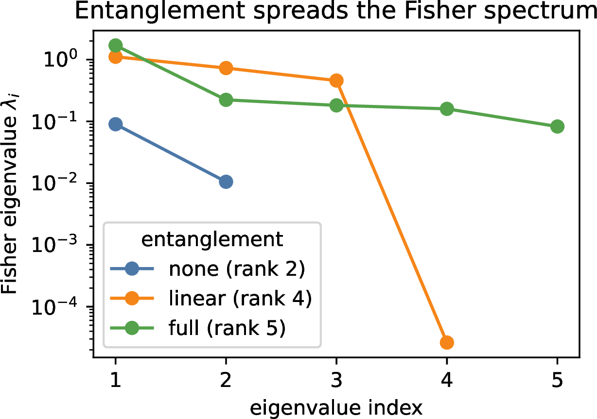
preserves it (\(0.034/0.065/0.089\)). In every control the entangled circuits generalize worse at identical parameter count. The mechanism is visible directly in the Fisher spectrum (Appendix 10, Figure 8): none has effectively two non-zero eigenvalues, linear three, and full five or more—entanglement raises the rank, hence \(d_{\mathrm{eff}}\).
7.0.0.2 Local vs.global readout: the effect is the readout light-cone, and \(d_{\mathrm{eff}}\) is the invariant.
The most adversarial test of the mechanism is also the most revealing. Because our single readout is the local observable \(\langle Z_0\rangle\), a rotation on a wire that never reaches qubit \(0\) has identically zero gradient (Lemma 2), so the unentangled none circuit is effectively a smaller model—only \(\sim\!d/n\) of its parameters are causally live. One might therefore object that “entanglement raises the gap at fixed \(d\)” is merely “entanglement recruits otherwise-dead parameters.” That
objection is correct, and it is the mechanism; we test it by the cleanest manipulation available—replacing the local readout by the global one \(\tfrac1n\sum_i\langle Z_i\rangle\), under which every wire
couples to the output directly (Table 6). The robust finding is that the global readout sharply raises none’s live-parameter count, \(d_{\mathrm{eff}}\), and gap at both
sizes— at \(n{=}4\) from \((2\text{ live},d_{\mathrm{eff}}{=}2.6,\text{gap}{=}{-}0.008)\) to \((7,14.0,0.095)\), at \(n{=}6\) from \((2,2.9,0.018)\) to \((11,23.6,0.173)\): the readout alone activates the parameters entanglement would have, and \(d_{\mathrm{eff}}\) and the gap move together. What happens to the full\(-\)none contrast is then \(n\)-dependent and
instructive. At \(n{=}4\) the single global observable nearly saturates the light-cone even for none (\(7\) of \(16\) live), so the entanglement
contrast is largely absorbed: full\(-\)none falls from \(+0.112\) (\(4.1\) s.e., local) to \(+0.033\) (\(0.9\) s.e., global). At \(n{=}6\), where \(24\) parameters cannot be saturated by one global observable
(none reaches \(11\) of \(24\) live, full \(17\)), entanglement still adds coupling on top and the contrast persists:
\(+0.114\) (\(3.8\) s.e., local) vs.\(+0.115\) (\(4.2\) s.e., global). The conclusion is therefore not that entanglement is
dispensable but that it is a readout-gated knob on the same underlying quantity: what governs \(d_{\mathrm{eff}}\) is how many parameters are causally coupled to the readout; a global readout raises the floor of
that coupling—fully absorbing the entanglement contrast at small \(n\), only partially at larger \(n\)—while in every cell it is \(d_{\mathrm{eff}}\), not the entangling label, that tracks the gap. This confirms Proposition 1 and sharpens the thesis: entanglement is the dominant,
structural driver of effective dimension for the local single-qubit Pauli readouts standard in quantum RL (e.g.[1], [2]), and is partly substitutable by—never orthogonal to—the choice of readout.
| \(n\) | readout | connectivity | live params | \(\Deff\) | gap |
|---|---|---|---|---|---|
| \(4\) | local \(\langle Z_0\rangle\) | none | \(2/16\) | \(2.6\) | \(-0.008\) |
| \(4\) | local \(\langle Z_0\rangle\) | full | \(5/16\) | \(12.9\) | \(0.104\) |
| \(4\) | global \(\tfrac1n\sum_i Z_i\) | none | \(7/16\) | \(14.0\) | \(0.095\) |
| \(4\) | global \(\tfrac1n\sum_i Z_i\) | full | \(12/16\) | \(30.7\) | \(0.128\) |
| \(6\) | local \(\langle Z_0\rangle\) | none | \(2/24\) | \(2.9\) | \(0.018\) |
| \(6\) | local \(\langle Z_0\rangle\) | full | \(7/24\) | \(21.1\) | \(0.132\) |
| \(6\) | global \(\tfrac1n\sum_i Z_i\) | none | \(11/24\) | \(23.6\) | \(0.173\) |
| \(6\) | global \(\tfrac1n\sum_i Z_i\) | full | \(17/24\) | \(35.4\) | \(0.289\) |
| full\(-\)none gap (\(n{=}4\)): local \(+0.112\) (\(4.1\sigma\)), | global \(+0.033\) (\(0.9\sigma\)) | ||||
| full\(-\)none gap (\(n{=}6\)): local \(+0.114\) (\(3.8\sigma\)), | global \(+0.115\) (\(4.2\sigma\)) | ||||
7.0.0.3 Beyond a single target.
To show the effect is not an artifact of one synthetic rule, we repeat the fixed-parameter-count comparison on three further targets (Table 7): a random-Fourier function, labels from an entangled teacher PQC, and \(4\)-bit parity. On the Fourier target the entangled circuits generalize above chance and the gap is again ordered none \(<\) linear \(<\) full. The entangled-teacher target is hard for all student circuits at this sample size (test accuracy near chance for every connectivity); we include it only as a stress test of gap behaviour—which still orders none \(<\) linear \(<\) full—and not as evidence of successful learning. Parity is the instructive exception and the clearest statement of the trade-off: it is not representable without entanglement, so the non-entangled and linear circuits sit at chance (\(0.50\)) while the all-to-all circuit is the only one that learns it (test accuracy \(0.90\)). Entanglement is therefore not uniformly harmful—when the target demands it, it is necessary—which is exactly why the right principle is to budget it, not to remove it.
| target | none gap (test) | linear gap (test) | full gap (test) |
|---|---|---|---|
| random Fourier | \(0.038\) (\(0.71\)) | \(0.045\) (\(0.69\)) | \(0.103\) (\(0.67\)) |
| entangled teacher | \(0.074\) (\(0.50\)) | \(0.123\) (\(0.50\)) | \(0.148\) (\(0.51\)) |
| \(4\)-bit parity | \(0.067\) (\(0.50\)) | \(0.116\) (\(0.50\)) | \(0.050\) (\(\mathbf{0.90}\)) |
7.0.0.4 Real (non-synthetic) benchmarks: entanglement lowers test accuracy.
The mechanism is not tied to a hand-designed rule, and on real data the cost shows up in test accuracy, not merely in the train–test gap. On standard small datasets—Iris, Breast Cancer (Wisconsin), Wine, and Digits (\(3\) vs.\(8\)), reduced to four features and binarized—the fixed-parameter-count comparison again orders the gap none \(<\) linear \(<\) full and co-monotone with \(d_{\mathrm{eff}}\) (Table 8). More importantly for the practical claim, on Wine and Digits the non-entangled circuit is significantly more accurate on held-out data than the all-to-all one, at accuracies far above chance: pooling over \(N\!\in\!\{16,24,32\}\) and \(22\) seeds, the test accuracy drops from \(0.884\) (none) to \(0.870\) (full) on Wine (\(2.5\) standard errors) and from \(0.911\) to \(0.900\) on Digits (\(3.1\) standard errors). Entanglement here genuinely hurts generalization on real tasks—not just widening the gap—which is what makes “budget entanglement” an operational, and not merely rhetorical, prescription.
| dataset | none gap (\(\Deff\), test) | linear gap (\(\Deff\), test) | full gap (\(\Deff\), test) |
|---|---|---|---|
| Iris | \(0.00\) (\(3.0\), \(0.70\)) | \(0.061\) (\(5.2\), \(0.65\)) | \(0.082\) (\(18.2\), \(0.76\)) |
| Breast Cancer | \(0.025\) (\(4.5\), \(0.90\)) | \(0.033\) (\(10.3\), \(0.91\)) | \(0.069\) (\(13.8\), \(0.90\)) |
| Wine | \(0.029\) (\(5.1\), \(0.90\)) | \(0.059\) (\(9.1\), \(0.88\)) | \(0.125\) (\(13.2\), \(0.85\)) |
7.0.0.5 The ordering holds where the model learns, and barren plateaus bound the mechanism.
Two concerns delimit the mechanism’s reach, and we test both directly. Is the ordering an artifact of the near-chance rows? We construct a deliberately learnable regime—\(n{=}6\), a lower-order target,
\(N{=}48\)—in which all three circuits reach held-out accuracy \(0.72\)–\(0.77\), far above the \(0.5\) chance level. The
ordering survives cleanly: the gap is \(0.042\) (none), \(0.043\) (linear), \(0.165\) (full), with
full\(-\)none\(=+0.123\) at \(5.8\) standard errors (\(8\) seeds) and \(d_{\mathrm{eff}}\) co-monotone (\(4.2/7.8/21.7\)). The effect is thus not confined to the degenerate near-chance rows—it is sharpest exactly where the circuits genuinely generalize.
Do barren plateaus erode the mechanism? Our mechanism runs on the Fisher spectrum, which barren plateaus flatten exponentially in qubit number, so the regime where scale matters is a natural worry. We confirm the erosion directly (Table 9): at a fixed moderate depth (\(L{=}4\), all-to-all, random parameters) the effective dimension falls monotonically from \(d_{\mathrm{eff}}{=}13.2\) at \(n{=}4\) to \(3.1\) at \(n{=}12\), even as the nominal parameter count rises from \(32\) to \(96\)—the Fisher eigenvalues shrink (the \(\langle Z_0\rangle\) gradient variance decays with \(n\)) faster than the rank grows, so \(d_{\mathrm{eff}}\) erodes toward its floor. This makes the boundary flagged in our failure-mode analysis (Appendix 9) quantitative: entanglement inflates \(d_{\mathrm{eff}}\) only while the circuit is off the plateau; deep or wide enough, barren plateaus drive \(d_{\mathrm{eff}}\)—and trainability itself—down together. The regime our claim and
design recipe target is therefore the trainable one (shallow circuits away from the plateau), which is where all our learning experiments sit.
| \(n\) | \(4\) | \(6\) | \(8\) | \(10\) | \(12\) |
|---|---|---|---|---|---|
| nominal params \(d\) | \(32\) | \(48\) | \(64\) | \(80\) | \(96\) |
| \(\Deff\) (\(L{=}4\), random) | \(13.2\) | \(8.4\) | \(4.5\) | \(3.2\) | \(3.1\) |
7.0.0.6 \(d_{\mathrm{eff}}\), not parameter count, is the stable predictor.
The complementary ablation—fixing the entangling pattern and varying depth, so the parameter count changes—shows the gap rising with depth for both patterns (linear: \(L{=}1{\to}4\) gap
\(0.03{\to}0.33\); full: \(0.03{\to}0.31\)), and in lock-step with \(d_{\mathrm{eff}}\) (which rises \(2{\to}50\) and \(2{\to}61\) respectively). At matched depth (matched parameter count) the more entangled pattern still has the larger \(d_{\mathrm{eff}}\) and
gap. Thus \(d_{\mathrm{eff}}\) predicts the gap whether we vary connectivity at fixed depth or depth at fixed connectivity, whereas raw parameter count only tracks the gap when it happens to co-vary with \(d_{\mathrm{eff}}\)—the sense in which \(d_{\mathrm{eff}}\), not parameter count, is the governing quantity.
7.0.0.7 End-to-end multi-step policy learning.
Finally, we train policies end-to-end by REINFORCE (with a value baseline, horizon \(8\), \(20\) seeds) on the multi-step return of an interaction-gated MDP—a genuine multi-step
policy-learning setting, not a value regression. Here the return generalization gap of the standard hardware-efficient (linear) entangler is significantly larger than the non-entangled circuit’s at the small \(N{=}8\) (\(0.62\) vs.\(0.16\), \(2.8\) standard errors over \(20\) seeds), directly confirming
the mechanism in end-to-end policy learning. The all-to-all circuit and the larger-\(N\) regime, however, are too high-variance to resolve (full-vs-none is within noise, and at \(N{=}16\)
all three are statistically indistinguishable): return-based estimates carry much more variance than the accuracy-based ones. We therefore report the significant linear-vs-none effect as genuine multi-step evidence, but continue
to treat the low-variance bandit and value-function settings as our primary probes of the mechanism.
7.0.0.8 The effect survives on real quantum hardware.
Finally we run the trained \(4\)-qubit classifiers on an IBM Heron device (ibm_aachen, \(156\) qubits) via the Estimator primitive at \(4096\) shots, reading \(\langle Z_0\rangle\) for all train and test inputs (Figure 6, right). Despite real gate and readout noise, the models run above chance and
the entanglement–generalization ordering is preserved: the gap is \(0.14\) for none versus \(0.33\) and \(0.31\) for linear and
full. The entanglement cost that our bound predicts is therefore not a simulation artifact—it is measurable on today’s hardware.
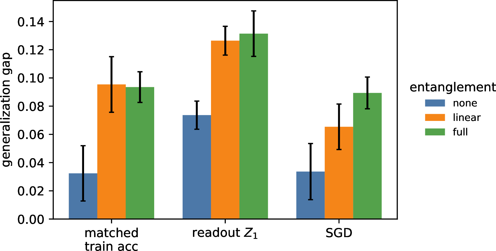
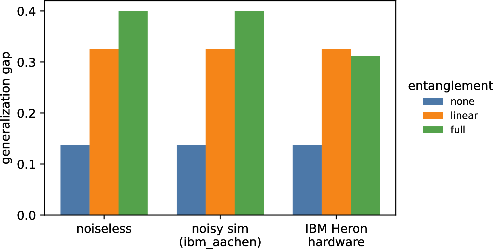
Figure 6: Left: the entangled-\(>\)-none gap ordering survives three controls at \(N{=}64\)—matched training accuracy, a different readout observable, and
a different optimizer—so the gap is not a mere optimization or trainability artifact. Right: the ordering is reproduced by a noise-model simulator of ibm_aachen and by execution on the ibm_aachen Heron processor
itself under real noise; calibration and shot-noise details are in Appendix 10..
Our bound is loose in absolute terms—like other PAC-Bayes bounds for expressive models it is most useful as a certificate that is valid, correctly ordered, and (where the gap is non-negligible) within \(\approx2.5\times\), rather than numerically tight. We frame entanglement as an independent and previously unisolated axis of complexity—the strongest single predictor of the gap in our study, ahead of the learned-norm term—though we do not claim it is the only one. The effect is depth-gated (a single entangling layer is inert for a single-qubit readout). Our RL evidence is for the one-step (contextual bandit) setting, chosen because full-MDP return estimates are dominated by trajectory-length variance; extending the clean measurement to multi-step MDPs—for example through offline value-function generalization—is the natural next step, along with value-based agents, hardware noise as an additional complexity channel, and a tight data-dependent prior. Our experiments are simulations of a controlled interaction task at \(n\in\{4,\dots,16\}\) qubits (Table 4); scaling to the many-qubit, hardware regime and to richer tasks is important future work, though the underlying mechanism—a light-cone argument—carries no dependence on \(n\).
7.0.0.9 A design recipe.
The trade-off is directly actionable as an ansatz-selection rule. Given a candidate ansatz family, estimate \(d_{\mathrm{eff}}\) on a small calibration set and choose the shallowest, sparsest entangling pattern whose training fit still improves a validation proxy without an excessive rise in \(d_{\mathrm{eff}}\). Concretely:
train each candidate ansatz to convergence on the calibration set;
compute its Fisher effective dimension \(d_{\mathrm{eff}}=\log\det(I+\gamma\hat{\mathcal{F}})\);
discard any ansatz whose \(d_{\mathrm{eff}}\) increases without a matching validation gain;
select from the Pareto frontier of validation performance versus \(d_{\mathrm{eff}}\).
This turns “budget entanglement” from a slogan into a concrete selection criterion—and, unlike a parameter budget, it distinguishes circuits of identical size.
8 Conclusion↩︎
We gave a PAC-Bayesian account of generalization for quantum policies in which the complexity that matters is the effective dimension of the circuit-induced Fisher geometry, a quantity inflated by entanglement and invisible to parameter counting. Isolating entanglement at fixed parameter count, we showed it is an independent predictor of the generalization gap—stronger than raw parameter count and comparable to the learned-norm term—across supervised classification, a reward-only contextual bandit, multi-step value-function generalization, and real quantum hardware. The resulting design principle—budget entanglement against its effective-dimension cost rather than maximize expressivity—gives quantum-policy design a target beyond average return.
Reproducibility Statement↩︎
Experiments use PQCs of \(n{=}4\) to \(16\) qubits simulated with PennyLane (default.qubit with backprop at \(n\le8\);
lightning.qubit with the adjoint method at \(n\ge10\)), plus one run on the IBM Heron ibm_aachen processor; unless a scaling experiment states otherwise (Table 4), the
default is \(n{=}4\). Code, ansätze, target/environment distributions, hyperparameters (\(\tau^2{=}1\), \(\gamma{=}50\)) and seeds are described in
Sections 4–6 and Appendix 10.
9 Proofs↩︎
9.1 Proof of Theorem 1↩︎
We reduce the return bound to the classical McAllester PAC-Bayes theorem. Recall its statement for a loss taking values in \([0,1]\).
Theorem 3 ([3]). Let \(\ell(h,z)\in[0,1]\), let \(z_1,\dots,z_m\) be i.i.d.from a distribution \(\mathcal{D}\), and let \(P\) be a prior over hypotheses chosen before seeing the data. For any \(\delta\in(0,1)\), with probability at least \(1-\delta\), simultaneously for all posteriors \(Q\), \[\mathbb{E}_{h\sim Q}\,\mathbb{E}_{z\sim\mathcal{D}}\,\ell(h,z) \;\le\; \mathbb{E}_{h\sim Q}\,\frac{1}{m}\sum_{i=1}^m \ell(h,z_i) +\sqrt{\frac{\mathrm{KL}(Q\Vert P)+\ln\frac{2\sqrt m}{\delta}}{2m}}.\]
Take the hypothesis \(h\) to be a parameter vector \(\theta\) (so \(Q,P\) are the Gaussians of Section 3), the sample \(z_i=M_i\) to be the \(i\)-th training environment drawn i.i.d.from \(\mathcal{D}\), and the loss to be the normalized regret of a single rollout, \(\ell(\theta,M)=1-R_M(\theta)/R_{\max}\in[0,1]\), where \(R_M(\theta)\) is the (bounded) return of \(\pi_\theta\) on \(M\). Then \(\mathbb{E}_{Q}\mathbb{E}_M \ell = 1-J(\pi_Q)/R_{\max}\) and its empirical counterpart is \(1-\hat{J}(\pi_Q)/R_{\max}\). Substituting into Theorem 3 and multiplying by \(R_{\max}\) gives \[J(\pi_Q)\;\ge\;\hat{J}(\pi_Q)-R_{\max}\sqrt{\frac{\mathrm{KL}(Q\Vert P)+\ln\frac{2\sqrt m}{\delta}}{2m}}.\] For a Gaussian posterior/prior with common covariance \(\sigma^2 I_d\), \(\mathrm{KL}(Q\Vert P)=\lVert\theta-\theta_0\rVert^2/(2\sigma^2)\), which is Eq. equation ?? with \(m_{\mathrm{eff}}=m\). When the per-environment return is instead estimated by pooling the \(T\) transitions of a trajectory—which are Markov-dependent rather than i.i.d.—the effective number of independent samples is reduced by the chain mixing factor, \(m_{\mathrm{eff}}=m/\kappa\) with \(\kappa=\Theta(t_{\mathrm{mix}})\), by the blocking argument of [5]; this yields the stated form. \(\square\)
9.2 Proof of Theorem 2↩︎
The KL divergence between two \(d\)-dimensional Gaussians \(Q=\mathcal{N}(\theta,\Sigma)\) and \(P=\mathcal{N}(\theta_0,\tau^2 I_d)\) is \[\mathrm{KL}(Q\Vert P)=\tfrac12\Big[\tfrac{1}{\tau^2}\operatorname{tr}\Sigma +\tfrac{1}{\tau^2}\lVert\theta-\theta_0\rVert^2-d-\log\det\tfrac{\Sigma}{\tau^2}\Big]. \label{eq:gausskl}\tag{2}\] Substitute the Gauss–Newton covariance \(\Sigma=\tau^2(I_d+\gamma\hat{\mathcal{F}})^{-1}\) and diagonalize \(\hat{\mathcal{F}}=\sum_i\lambda_i u_iu_i^\top\). Then \(\tfrac{1}{\tau^2}\operatorname{tr}\Sigma=\sum_i(1+\gamma\lambda_i)^{-1}\), \(\log\det\tfrac{\Sigma}{\tau^2}=-\sum_i\log(1+\gamma\lambda_i)\), and using \(d=\sum_i 1=\sum_i\big[(1+\gamma\lambda_i)^{-1}+\tfrac{\gamma\lambda_i}{1+\gamma\lambda_i}\big]\) the trace and \(-d\) terms combine to \(-\sum_i\tfrac{\gamma\lambda_i}{1+\gamma\lambda_i}\). Collecting terms, \[\mathrm{KL}(Q\Vert P)=\frac{\lVert\theta-\theta_0\rVert^2}{2\tau^2} +\tfrac12\sum_i\log(1+\gamma\lambda_i) -\tfrac12\sum_i\frac{\gamma\lambda_i}{1+\gamma\lambda_i},\] which is equation ?? since \(\sum_i\log(1+\gamma\lambda_i)=\log\det(I_d+\gamma\hat{\mathcal{F}})=d_{\mathrm{eff}}(\gamma)\). Each summand of the last term lies in \([0,\tfrac12)\), so \(0\le\tfrac12\sum_i\tfrac{\gamma\lambda_i}{1+\gamma\lambda_i}\le d/2\) and dropping it can only enlarge the right-hand side of the bound. The prior \(P\) is fixed at initialization \(\theta_0\) and does not depend on the training environments, so Theorem 3 applies verbatim with this \(Q\) and \(P\); substituting the resulting KL into the return bound of Theorem 1 gives equation ?? . The asymptotics \(d_{\mathrm{eff}}(\gamma)\le d\) and \(d_{\mathrm{eff}}(\gamma)=\mathrm{rank}(\hat{\mathcal{F}})\log\gamma+O(1)\) as \(\gamma\to\infty\) follow from \(\log(1+\gamma\lambda_i)\le\gamma\lambda_i\) and, for \(\lambda_i>0\), \(\log(1+\gamma\lambda_i)=\log\gamma+\log\lambda_i+o(1)\). \(\square\)
9.3 Derandomization: from the stochastic \(\pi_Q\) to the deterministic \(\theta\)↩︎
The bound equation ?? controls the gap of the posterior-averaged predictor \(\pi_Q\), whereas the reported “true gap” is that of the deterministic trained \(\theta\). The following lemma bounds the difference and, crucially, shows the flat Fisher directions—which carry the full prior variance \(\tau^2\)—do not spoil it, because the perturbation of a loss along a direction is weighted by that direction’s curvature, which is the Fisher eigenvalue itself.
Lemma 1 (Flat-direction derandomization). Let \(Q=\mathcal{N}(\theta,\Sigma)\) with \(\Sigma=\tau^2(I_d+\gamma\hat{\mathcal{F}})^{-1}\), and let \(L(\vartheta)=\mathbb{E}_s\,\ell(\vartheta,s)\) be a population loss whose Hessian at \(\theta\) equals the Fisher \(\hat{\mathcal{F}}(\theta)\) up to a residual term \(\mathcal{R}\) that is \(O(\lVert p-y\rVert)\) and vanishes in the Gauss–Newton (well-fit) regime. Then \[\big|\,\mathbb{E}_{\vartheta\sim Q}\,L(\vartheta)-L(\theta)\,\big| \;=\;\tfrac12\,\mathrm{tr}\!\big(\Sigma\,\hat{\mathcal{F}}\big)+O(\lVert\Sigma\rVert^{3/2}) \;=\;\frac{\tau^2}{2}\sum_{i=1}^d\frac{\lambda_i}{1+\gamma\lambda_i}\;+\;O(\lVert\Sigma\rVert^{3/2}), \label{eq:derand}\qquad{(4)}\] and the sum is bounded by \(\dfrac{1}{\gamma}\cdot\dfrac12\sum_i\dfrac{\gamma\lambda_i}{1+\gamma\lambda_i}\le\dfrac{d}{2\gamma}\). Consequently the train and test losses of \(\pi_Q\) and of \(\theta\) each differ by at most \(\tfrac12\tau^2\sum_i\lambda_i/(1+\gamma\lambda_i)\le\tau^2 d/(2\gamma)\), so the two generalization gaps differ by at most \(\tau^2\sum_i\lambda_i/(1+\gamma\lambda_i)\le\tau^2 d/\gamma\).
Proof. Since \(\mathbb{E}_{\vartheta\sim Q}[\vartheta-\theta]=0\), a second-order Taylor expansion of \(L\) about \(\theta\) gives \(\mathbb{E}_Q L(\vartheta)-L(\theta)=\tfrac12\,\mathbb{E}_Q[(\vartheta-\theta)^\top\nabla^2 L\,(\vartheta-\theta)]+O(\lVert\Sigma\rVert^{3/2}) =\tfrac12\mathrm{tr}(\Sigma\nabla^2 L)+O(\lVert\Sigma\rVert^{3/2})\), the remainder controlled by the third derivative of the smooth PQC expectation and the Gaussian third moment. For the logistic head, \(\nabla^2 L=\mathbb{E}_s[\alpha^2 p_s(1{-}p_s)\nabla f_s\nabla f_s^\top] +\mathbb{E}_s[\alpha(p_s{-}y_s)\nabla^2 f_s]=\hat{\mathcal{F}}+\mathcal{R}\), and \(\mathcal{R}\) vanishes as the fit improves (\(p_s\!\to\!y_s\)). Substituting \(\Sigma=\tau^2(I_d+\gamma\hat{\mathcal{F}})^{-1}\) and diagonalizing \(\hat{\mathcal{F}}\) gives \(\mathrm{tr}(\Sigma\hat{\mathcal{F}})=\tau^2\sum_i\lambda_i/(1+\gamma\lambda_i)\), which is equation ?? . Writing \(\lambda_i/(1+\gamma\lambda_i)=\gamma^{-1}\cdot\gamma\lambda_i/(1+\gamma\lambda_i)\) and \(\gamma\lambda_i/(1+\gamma\lambda_i)\in[0,1)\) gives the \(d/2\gamma\) envelope. A flat direction (\(\lambda_i\!\to\!0\)) contributes \(\lambda_i/(1+\gamma\lambda_i)\!\to\!\lambda_i\!\to\!0\) despite its posterior variance \(\Sigma_{ii}\!\to\!\tau^2\): the variance is large but the curvature that converts it into a loss change is exactly \(\lambda_i\), so flat directions are harmless. The gap statement follows by applying the bound to the train and test losses separately and using the triangle inequality. ◻
Note that the derandomization cost \(\tfrac12\tau^2\sum_i\lambda_i/(1+\gamma\lambda_i)\) is exactly \(1/\gamma\) times the KL curvature term \(\tfrac12\sum_i\gamma\lambda_i/(1+\gamma\lambda_i)\) that we dropped in Eq. equation ?? : the same quantity we discarded to expose \(d_{\mathrm{eff}}\) reappears, scaled by \(1/\gamma\), as the price of derandomization, and \(\gamma{=}50\) makes it small (\(\le d/100\) for \(\tau^2{=}1\)). This ties the two approximations together and replaces the informal “low-temperature” argument in the main text.
9.4 Proof of Proposition 1↩︎
Write the readout expectation in the Heisenberg picture, \(f(s,\theta)=\langle\psi(s)|\,U(\theta)^\dagger Z_0\, U(\theta)\,|\psi(s)\rangle\), and let gate \(i\) be a Pauli rotation \(e^{-\mathrm{i}\theta_i G_i/2}\) with \(G_i\) a single-qubit Pauli on wire \(q(i)\). Splitting the circuit at gate \(i\) as \(U=U_{>i}\,e^{-\mathrm{i}\theta_i G_i/2}\,U_{\le i}\) and defining the back-propagated observable \(O_i(\theta)=U_{>i}^\dagger Z_0\,U_{>i}\), the parameter-shift identity gives \[\partial_{\theta_i} f(s,\theta) =-\tfrac{\mathrm i}{2}\,\langle\phi_i(s)|\,[\,G_i,\,O_i(\theta)\,]\,|\phi_i(s)\rangle, \qquad |\phi_i(s)\rangle=U_{\le i}|\psi(s)\rangle . \label{eq:pshift}\tag{3}\] The (output-)Fisher matrix is \(\hat{\mathcal{F}}_{ij}=\mathbb{E}_s[\,c(s)\,\partial_{\theta_i} f\,\partial_{\theta_j} f\,]\) with \(c(s)=\mathrm{sc}^2 p(1{-}p)>0\), so \(\hat{\mathcal{F}}=\mathbb{E}_s[c(s)\,g_s g_s^\top]\) where \(g_s=\nabla_\theta f(s,\theta)\); in particular \(\mathrm{rank}(\hat{\mathcal{F}})\le|\{i:\;\partial_{\theta_i} f\not\equiv 0\}|\), with equality generically.
Definition 1 (Backward light-cone). Let \(\mathcal{L}(\theta)\subseteq\{1,\dots,d\}\) be the set of parameters \(i\) for which \(O_i(\theta)\) has non-trivial support on wire \(q(i)\), i.e.\([G_i,O_i(\theta)]\neq 0\).
Lemma 2 (Entanglement enlarges the light-cone). Fix the placement of all rotation gates. If a set of two-qubit entangling gates is added to the circuit (keeping all rotations), then \(\mathcal{L}(\theta)\) can only grow: \(\mathcal{L}_{\mathrm{without}}(\theta)\subseteq\mathcal{L}_{\mathrm{with}}(\theta)\) for generic \(\theta\). In particular, with no entangling gates \(O_i(\theta)\) is supported on wire \(0\) alone, so \([G_i,O_i]=0\) for every rotation on a wire \(q(i)\neq 0\) and \(\mathcal{L}=\{i:q(i)=0\}\).
Proof. \(O_i(\theta)=U_{>i}^\dagger Z_0 U_{>i}\) is \(Z_0\) conjugated by the gates after \(i\). Each single-qubit rotation preserves the support of an operator on its own wire; each two-qubit gate can only enlarge support to the wires it couples. Hence the support of \(O_i\) is contained in the causal cone of \(Z_0\) under the gates in \(U_{>i}\), which is monotone non-decreasing under the addition of entangling gates. With no entangling gates the cone is \(\{0\}\), so \(O_i\) commutes with any \(G_i\) on a different wire, giving \(\partial_{\theta_i}f\equiv0\) by equation 3 . Adding entangling gates that reach wire \(q(i)\) makes \(O_i\) act non-trivially there, so \([G_i,O_i]\neq0\) for generic \(\theta\) and \(i\) enters \(\mathcal{L}\). ◻
Assumption 1 (Genericity). For generic parameters the nonzero gradients \(\{g_s\}\) span \(\mathrm{span}\{e_i:i\in\mathcal{L}(\theta)\}\) and the induced Fisher eigenvalues on this subspace are of comparable magnitude (no exact degeneracies or cancellations).
Proof of Proposition 1. The rank identity \(\mathrm{rank}(\hat{\mathcal{F}})=|\{i:\partial_{\theta_i}f\not\equiv0\}|=|\mathcal{L}(\theta)|\) holds because \(\hat{\mathcal{F}}=\mathbb{E}_s[c(s)g_sg_s^\top]\) is supported on \(\mathrm{span}\{e_i:i\in\mathcal{L}(\theta)\}\) (parameters outside the light-cone have \(\partial_{\theta_i}f\equiv0\) by Lemma 2 and equation 3 ), and by Assumption 1 the in-cone gradients span that subspace, so the inequality is an equality. Monotonicity of \(|\mathcal{L}(\theta)|\) in the entangling connectivity is Lemma 2. Because \(d_{\mathrm{eff}}(\gamma)=\sum_i\log(1+\gamma\lambda_i)\) receives a contribution only from the \(\mathrm{rank}(\hat{\mathcal{F}})\) nonzero eigenvalues and \(d_{\mathrm{eff}}(\gamma)=\mathrm{rank}(\hat{\mathcal{F}})\log\gamma+O(1)\) for large \(\gamma\), any increase of \(\mathrm{rank}(\hat{\mathcal{F}})\) raises \(d_{\mathrm{eff}}(\gamma)\) at fixed \(d\). Hence increasing entangling connectivity raises \(d_{\mathrm{eff}}\) while \(d\) is fixed. ◻
The empirical counterpart is Table 10: at fixed depth (fixed \(d\)) the measured \(d_{\mathrm{eff}}=\log\det(I+\gamma\hat{\mathcal{F}})\) rises monotonically from its no-entanglement value (none \(\to\) linear \(\to\) full), tracking the rank of the Fisher matrix.
9.4.0.1 Scope, a worked example, and failure modes.
We state precisely what Proposition 1 does and does not give. Scope. It applies to hardware-efficient ansätze in which (a) each trainable gate is a Pauli rotation, (b) the readout is a fixed Pauli observable, and (c) encoding gates precede the trainable block. The two claims have different strengths: rank monotonicity (\(\mathrm{rank}(\hat{\mathcal{F}}_{\mathrm{with}})\ge\mathrm{rank}(\hat{\mathcal{F}}_{\mathrm{without}})\)) is rigorous—it is Lemma 2 plus the support argument, with no genericity needed for the inequality (genericity is used only to turn it into the equality \(\mathrm{rank}=|\mathcal{L}|\)). The stronger effective-dimension monotonicity \(d_{\mathrm{eff}}(\gamma)_{\mathrm{with}}\ge d_{\mathrm{eff}}(\gamma)_{\mathrm{without}}\) holds unconditionally only as \(\gamma\to\infty\) (where \(d_{\mathrm{eff}}\!\to\!\mathrm{rank}\cdot\log\gamma\)); at finite \(\gamma\) a rank increase raises \(d_{\mathrm{eff}}\) provided the new eigenvalues are not vanishingly small, since \(d_{\mathrm{eff}}=\sum_i\log(1+\gamma\lambda_i)\) and a mode with \(\lambda\!\approx\!0\) contributes \(\approx0\). We therefore separate the two in the statement.
Worked example. Take \(n{=}2\) qubits, one layer, readout \(Z_0\), trainable \(R_Y(\theta_0)\) on qubit \(0\) and \(R_Y(\theta_1)\) on qubit \(1\). Without a CNOT, \(\partial_{\theta_1}\langle Z_0\rangle\equiv0\) (the back-propagated observable is \(Z_0\!\otimes\!I\), which commutes with \(Y_1\)), so \(\hat{\mathcal{F}}=\mathrm{diag}(c\,\langle\dots\rangle,0)\) has rank \(1\). Inserting \(\mathrm{CNOT}_{0\to1}\) before the readout maps \(Z_0\mapsto Z_0\) but \(\mathrm{CNOT}_{1\to0}\) maps \(Z_0\mapsto Z_0Z_1\), which no longer commutes with \(Y_1\); then \(\partial_{\theta_1}\langle Z_0\rangle=-\tfrac{\mathrm i}{2}\langle[Y_1,Z_0Z_1]\rangle\neq0\) generically and \(\mathrm{rank}(\hat{\mathcal{F}})=2\). This is the mechanism in closed form.
Failure modes. The rank does not increase when the added entanglement is neutralized by structure: (i) a symmetry or commuting-gate configuration for which \([G_i,O_i(\theta)]=0\) despite non-trivial support (e.g.\(O_i\) proportional to \(Z_{q(i)}\) and \(G_i=Z_{q(i)}\)); (ii) fine-tuned parameters at which the new gradients vanish (a measure-zero set excluded by genericity); and (iii) the barren-plateau regime, where all \(\lambda_i\!\to\!0\) exponentially, so although the rank may rise the finite-\(\gamma\) \(d_{\mathrm{eff}}\) stays near zero—entanglement then inflates capacity only once the circuit is trained away from the plateau. These are exactly the cases our experiments avoid (shallow circuits, generic trained parameters), and they delimit the claim.
10 Additional experimental detail↩︎
10.0.0.1 Setup.
All PQCs use \(n{=}4\) qubits simulated with PennyLane’s default.qubit and a single readout observable \(\langle Z_0\rangle\). Inputs are angle-encoded with \(R_Y\); the ansatz is \(L\) layers of \(R_Y,R_Z\) per qubit (\(d{=}2nL\) trainable angles) followed by a fixed CNOT pattern
(none/linear/full). Figure 7 shows the three ansätze: they share the identical rotation layout (hence \(d\)) and differ only in the entangling block.
Supervised models (Sections 4–5) are binary classifiers \(\hat{y}=\mathrm{sign}(\langle Z_0\rangle)\) trained by Adam (\(600\) steps, full batch, lr \(0.08\)) with the cross-entropy loss on the interaction target \(y=\mathrm{sign}(x_1x_2-x_3x_4+\tfrac12 x_1)\), \(x\sim U[-1,1]^4\), and evaluated on \(2000\) held-out inputs. RL policies (Section 6) are contextual-bandit policies \(\pi(a{=}1\mid x)=\sigma(\alpha\langle Z_0\rangle)\) over contexts \(x\sim U[-1,1]^4\), trained by REINFORCE (\(600\) updates, lr \(0.08\)) on bandit feedback (reward \(1\) iff the sampled action equals \(a^\star(x)=\mathbb{1}[x_1x_2-x_3x_4+\tfrac12 x_1>0]\), the correct label is never revealed); the gap is training reward minus reward on \(2000\) held-out contexts. Each cell averages \(8\) (supervised) or \(16\) (bandit) seeds. The Meyer–Wallach \(Q\) and the Fisher matrix are evaluated at the trained parameters over held-out inputs.
10.0.0.2 Fisher effective dimension: exact computation.
To remove ambiguity we specify the estimator precisely. (i) We use the empirical output Fisher of the policy’s Bernoulli head, not the parameter/loss Fisher and not the exact Fisher: \(\hat{\mathcal{F}}(\theta)=\tfrac1M\sum_{x} c(x)\,g_x g_x^\top\) with \(g_x=\nabla_\theta\langle Z_0\rangle_{x,\theta}\) and Bernoulli weight \(c(x)=\alpha^2\,p(x)(1{-}p(x))\), \(p=\sigma(\alpha\langle Z_0\rangle)\). (ii) It is evaluated at the trained parameters \(\theta\) over \(M{=}40\) held-out inputs drawn from the input distribution (not the training set). (iii) The per-input gradients \(g_x\) are computed by autograd (exact parameter-shift). (iv) Eigenvalues \(\lambda_i\) of \(\hat{\mathcal{F}}\) are used unnormalized (no trace rescaling). (v) The effective dimension is \(d_{\mathrm{eff}}=\log\det(I+\gamma\hat{\mathcal{F}})=\sum_i\log(1+\gamma\lambda_i)\) with the constant \(\gamma=50\) used identically everywhere (Remark 1). (vi) For a reported cell we compute \(d_{\mathrm{eff}}\) per seed and then average \(d_{\mathrm{eff}}\) across seeds (we do not pool the Fisher matrices). The participation ratio \((\sum_i\lambda_i)^2/\sum_i\lambda_i^2\), when reported, is computed from the same spectra. Why \(\gamma{=}50\), and does it matter. The value \(50\) places the observed spectra (eigenvalues \(\lambda\!\in\![10^{-2},2]\)) in the informative band where \(\gamma\lambda\) spans \(\approx0.5\)–\(100\), so \(d_{\mathrm{eff}}\) is neither saturated nor collapsed to zero. Crucially the conclusions we draw from \(d_{\mathrm{eff}}\) are insensitive to this choice, since \(d_{\mathrm{eff}}(\gamma)=\sum_i\log(1+\gamma\lambda_i)\) is monotone in the Fisher spectrum. We recomputed \(d_{\mathrm{eff}}\) for all \(18\) configurations of Table 2 at \(\gamma\in\{10,25,50,100,200\}\): the Spearman correlation \(\rho(d_{\mathrm{eff}},\mathrm{gap})\) is \(0.74,0.70,0.67,0.67,0.64\) respectively—stable in sign and magnitude—and the ordering none \(<\) linear \(<\) full holds at every \(\gamma\) (e.g.at \(L{=}2\), \(d_{\mathrm{eff}}\) goes \(2.5{\to}4.8{\to}11.5\) at \(\gamma{=}10\) and \(5.8{\to}12.2{\to}25.6\) at \(\gamma{=}200\)). We fix a single \(\gamma=50\) only so that \(d_{\mathrm{eff}}\) is numerically comparable across rows.
10.0.0.3 \(d_{\mathrm{eff}}\) dominates the learned norm—a powered, bootstrapped test.
A comparison between two correlations of \(0.76\) and \(0.70\) over \(18\) points would be underpowered, so we built a much larger and more varied grid:
\(5\) entangling patterns (none/linear/ring/alt/full) \(\times\) depths \(L\!\in\!\{1,\dots,5\}\) \(\times\) \(N\!\in\!\{16,32,64\}\) \(\times\) \(4\) seeds \(=300\) configurations, which dissociates \(d_{\mathrm{eff}}\) from the learned norm and from parameter count. Across these \(300\) points the Spearman
correlations with the gap are \(\rho(d_{\mathrm{eff}})=0.82\), \(\rho(\lVert\theta{-}\theta_0\rVert^2)=0.73\), \(\rho(Q)=0.72\), \(\rho(\text{params})=0.45\). A \(5000\)-resample bootstrap over configurations gives \(\Delta\rho=\rho(d_{\mathrm{eff}})-\rho(\text{norm})=0.090\) with \(95\%\) CI \([0.041,0.144]\) (bootstrap \(P(\Delta\rho{>}0){=}1.00\)), and \(\rho(d_{\mathrm{eff}})-\rho(Q)=0.100\), CI \([0.046,0.156]\): the Fisher effective dimension is a significantly better predictor of the gap than the learned norm or the entangling power. A multiple regression on the same grid loads almost entirely on \(d_{\mathrm{eff}}\) (standardized coefficient \(+0.16\) vs.\(\le0.06\) in magnitude for the others), and adding the entangling pattern on top of \(d_{\mathrm{eff}}\) raises \(R^2\) by \(<0.01\) while adding \(d_{\mathrm{eff}}\) on top of the pattern raises it by \(0.14\). Entanglement therefore acts on the gap through \(d_{\mathrm{eff}}\), which screens it off—the precise, and now powered, sense in which \(d_{\mathrm{eff}}\) is the governing quantity.
10.0.0.4 Fisher effective dimension and gap, per configuration.
Table 10 gives the Fisher effective dimension \(d_{\mathrm{eff}}=\log\det(I+\gamma\hat{\mathcal{F}})\) (Eq. equation 1 , fixed \(\gamma=50\)) and the gap for every connectivity at depths \(L{=}2,3\) and \(N_{\mathrm{train}}{=}16\). At fixed depth (fixed \(d\)), \(d_{\mathrm{eff}}\) increases monotonically with entangling connectivity, and so does the gap.
| depth | connectivity | \(N_{\mathrm{train}}\) | Fisher \(\Deff\) (log-det) | gap |
|---|---|---|---|---|
| \(L{=}2\) | none | \(16\) | \(3.3\) | \(0.101\) |
| \(L{=}2\) | linear | \(16\) | \(9.3\) | \(0.146\) |
| \(L{=}2\) | full | \(16\) | \(21.8\) | \(0.381\) |
| \(L{=}3\) | none | \(16\) | \(4.0\) | \(0.101\) |
| \(L{=}3\) | linear | \(16\) | \(29.5\) | \(0.440\) |
| \(L{=}3\) | full | \(16\) | \(36.5\) | \(0.431\) |
The ordering none \(<\) linear \(<\) full holds for both \(d_{\mathrm{eff}}\) and the gap at \(L{=}2\) and \(L{=}3\); a single entangling layer (\(L{=}1\)) leaves the gap unchanged, the depth-gating referred to in the main text.
10.0.0.5 Multi-step value-function generalization and controls.
The value-function experiment (Section 6) fits a single-observable VQC to \(V^\star(x)=\sum_{t=0}^{5}0.9^{t}r(x_t)\) under the deterministic transition \(x'=\tanh(1.3\,\mathrm{roll}(x)+0.2x)\) with \(r\) the interaction rule, by Adam regression (\(800\) steps) on \(N\) states,
reporting held-out \(R^2\) over \(1000\) states. The controls of Section 7 use \(N{=}64\): matched-accuracy early-stops
at train accuracy \(0.72\); the readout control measures \(Z_1\); the optimizer control uses SGD (lr \(0.5\)). The hardware run trains the \(N{=}16\) classifiers in simulation and evaluates \(\langle Z_0\rangle\) for all \(56\) inputs on ibm_aachen via EstimatorV2 at \(4096\) shots, optimization level \(1\).
10.0.0.6 Hardware credibility: calibration, noise, and shot statistics.
The device is IBM Heron ibm_aachen (\(156\) qubits). At the time of execution its median two-qubit gate error was \(1.8\times10^{-3}\) (typical range \(7\times10^{-4}\) to a few \(\times10^{-3}\), excluding one inoperable pair) and median \(T_1\approx218\,\mu\)s. Readout error mitigation was not
applied—the effect we report survives raw device noise. Three cross-checks support the hardware numbers (Figure 6, right). (i) A noise-model simulator built from the ibm_aachen calibration
(AerSimulator with NoiseModel.from_backend) reproduces the ordering (gap \(0.14/0.33/0.40\) for none/linear/full), i.e.the modelled noise does not remove the effect. (ii) Shot noise is
small: at \(4096\) shots each \(\langle Z_0\rangle\) estimate has standard error \(\approx\!1/\sqrt{4096}\approx0.016\), which flips a sign only for inputs
within that margin of the decision boundary, so the accuracy-based gap is stable. (iii) The raw hardware gaps (\(0.14/0.33/0.31\)) agree with both the noiseless and noise-model values to within \(\approx0.1\), and preserve the none \(<\) ordering. We report the hardware result as corroboration of the simulation evidence, not as a separate quantitative claim.
10.0.0.7 Compute and reproducibility.
All classical simulations use PennyLane default.qubit with the PyTorch interface (analytic gradients). Each supervised cell averages \(8\) seeds, each bandit/robustness/real-data cell \(16\)/\(8\)/\(6\) seeds, and the value-function and policy-gradient cells \(8\)/\(10\) seeds;
error bars are one standard error. Targets: interaction rule \(\mathrm{sign}(x_1x_2{-}x_3x_4{+}\tfrac12 x_1)\) (main); \(4\)-bit parity \(\mathrm{sign}(\prod_i
\mathrm{sign}(x_i))\); random Fourier \(\mathrm{sign}(\sum_{k=1}^{6}\cos(w_k\!\cdot\!x+b_k))\) with fixed \(w_k,b_k\); entangled-teacher labels \(\mathrm{sign}(\langle Z_0\rangle)\) of a fixed \(2\)-layer StronglyEntangling teacher. Real datasets are the scikit-learn Iris (versicolor vs.virginica), Breast Cancer Wisconsin,
and Wine (classes \(0\)/\(1\)) sets, standardized, reduced to four features by PCA when needed, and min–max scaled to \([-1,1]\).