Canopy: A Heterograph Foundation Model for Metabolic Engineering
July 07, 2026
Abstract
Designing microbial strains that produce high-value chemicals at commercially viable titers remains a central challenge in metabolic engineering. Existing computational approaches either rely on stoichiometric constraint-based models that cannot learn from experimental data, or apply tabular machine learning to hand-crafted features that discard the relational structure of biological knowledge. We present Canopy, a heterogeneous graph foundation model that integrates ten public and proprietary data sources into a unified knowledge graph (KG) of 6.9 M nodes across 13 types and 34 edge types, covering genes, proteins, metabolites, reactions, pathways, strains, and fermentation experiments. Node features are encoded through domain-specific foundation models (ESM-2 for protein sequences, MoLFormer for chemical SMILES, and PubMedBERT for biomedical text), yielding a multi-modal representation within a single graph. We pretrain a Heterogeneous Graph Transformer (HGT) augmented with SignNet positional encodings, Jumping Knowledge aggregation, and virtual nodes using four self-supervised objectives (link prediction, masked node modelling, distance prediction, and contrastive experiment clustering), balanced via learned homoscedastic uncertainty weighting. On the downstream task of fermentation titer prediction, frozen Canopy embeddings achieve \(R^{2} = 0.41\) with a lightweight probe, outperforming tabular baselines (best \(R^{2} = 0.24\)) and homogeneous GNN variants.
1 Introduction↩︎
The bioeconomy depends on engineered microorganisms that convert renewable feedstocks into fuels, pharmaceuticals, and specialty chemicals. The design–build–test–learn (DBTL) cycle that underpins strain engineering is slow: a single round of genetic modification, fermentation, and analytical characterisation can take weeks to months [1], and the combinatorial space of candidate modifications grows exponentially in the number of target genes. Computational tools that prioritise genetic interventions before wet-lab experiments would shorten this loop.
The dominant computational paradigm for strain design is constraint-based modelling via genome-scale metabolic models (GEMs). Flux balance analysis (FBA) and its extensions predict steady-state fluxes under stoichiometric and thermodynamic constraints, enabling in silico knockout analysis through tools such as OptKnock [2] and StrainDesign [3]. While GEMs encode mechanistic knowledge of metabolism, they cannot incorporate experimental measurements of titer, rate, and yield; they ignore regulatory, expression-level, and environmental effects; and they treat each organism in isolation without using cross-organism transfer.
Machine learning offers a complementary approach. Previous work has applied random forests, gradient boosting, and neural networks to predict fermentation titer from features extracted from strain descriptions [4], [5]. These tabular approaches discard the relational structure that links genes to proteins, proteins to reactions, reactions to pathways, and pathways to production phenotypes. Graph neural networks have been applied to metabolic networks for gene essentiality [6] and site-of-metabolism prediction [7], but these operate on single-organism reaction graphs rather than on cross-organism knowledge graphs.
Meanwhile, the broader ML community has advanced heterogeneous graph transformers [8], self-supervised graph pretraining [9], and domain-specific foundation models for proteins [10] and small molecules [11]. Biomedical knowledge graphs such as PrimeKG [12] have enabled GNN-based drug repurposing, but no analogous resource or foundation model exists for the metabolic engineering domain, which sits at the intersection of microbial genetics, enzyme biochemistry, and fermentation science.
We introduce Canopy, a heterogeneous graph foundation model for metabolic engineering. Our contributions are:
A metabolic-engineering knowledge graph integrating ten data sources (MetaNetX, GO, UniRef, InterPro, NCBI Taxonomy and Genomics, KEGG, an in-house laboratory information management system (LIMS) of unpublished DBTL records, literature-mined experiments, and transcriptomics) via BioCypher [13] into a unified heterogeneous graph with 13 node types and 34 edge types.
Multi-modal feature encoding using a schema-driven dispatch system that routes protein sequences to ESM-2 (650M), SMILES strings to MoLFormer-XL, free text to PubMedBERT, and numeric features to normalised scalars within a single graph.
An augmented Heterogeneous Graph Transformer combining HGTConv with SignNet positional encodings, random walk structural encodings, per-type feed-forward networks (FFNs) with learnable residual scaling, Jumping Knowledge aggregation, and virtual nodes.
Four-objective self-supervised pretraining with learned uncertainty weighting: link prediction, masked node modelling, distance prediction, and a contrastive experiment-pair loss.
Downstream evaluation on fermentation titer prediction, showing that learned graph representations outperform tabular baselines and provide the conditioning substrate for downstream generative strain-design pipelines.
2 Related Work↩︎
2.0.0.1 Foundation models across biological scales.
Domain-specific foundation models now span genomes [14], [15], protein sequence [10], [16] and structure [17], [18], molecules [11], and single-cell transcriptomics [19], [20]. Each captures a single modality at a single scale; none are jointly trained over the relational structure that links genes to enzymes to metabolites to fermentation outcomes. Canopy embeds frozen ESM-2, MoLFormer, and PubMedBERT features inside a heterogeneous KG, treating these models as feature encoders within a graph that crosses scales.
2.0.0.2 Predictive and generative models for strain, pathway, and enzyme design.
Kinetic GEMs such as k-ecoli457 [21] extend FBA with parameterised rate equations fit to fluxomic data and predict product yields more accurately than purely stoichiometric models, but their parameterisation is organism-specific and does not transfer across strains. Tabular ML on hand-crafted features remains dominant for titer prediction [4], [5], [22]; graph methods so far have been single-organism [6], [23] or relied on shallow KG embeddings [24], [25]. Diffusion- and flow-matching-based generative models are seeing rapid uptake for protein backbones and enzyme active sites [26], [27], but target single molecules rather than whole-strain phenotypes. Canopy predicts titer from a learned cross-organism representation that fuses sequence, chemistry, and KG context. The same frozen embeddings can condition a downstream Bayesian-optimisation loop [28] or generative model.
2.0.0.3 Benchmarks for ML in metabolic engineering.
A useful benchmark for ML-driven metabolic engineering needs three things: experimental titer measurements, cross-organism coverage, and multi-omic context for each strain. No existing resource provides all three. SimDBTL [29] offers consistent DBTL splits but its data are simulated rather than experimental. Therapeutics Data Commons [30] standardises prediction splits for therapeutic rather than fermentation tasks. Text-mining catalogues of over 15,000 strain-design publications [31] surface raw records without a held-out evaluation. Canopy’s 4,791 fermentation experiments with a deterministic MD5-hashed 5x CV split address all three criteria.
2.0.0.4 Biological knowledge graphs and heterogeneous GNNs.
Large biomedical KGs (PrimeKG, [12]; Hetionet, [32]; SPOKE, [33]) and graph foundation models built on them [34], [35] target human disease, not metabolic engineering. We use BioCypher [13] to integrate ten metabolic-engineering adapters and build on the Heterogeneous Graph Transformer [8] with SignNet [36], random-walk PE [37], Jumping Knowledge [38], and virtual nodes [39]; pretraining objectives draw on [9] and the graph-FM surveys of [40], [41]. The closest cross-organism transfer is IKT4Meta [23]; Canopy extends this from two-organism alignment to a 13-node-type, multi-modal KG with fermentation-scale supervision.
3 Method↩︎
3.1 Knowledge Graph Construction↩︎
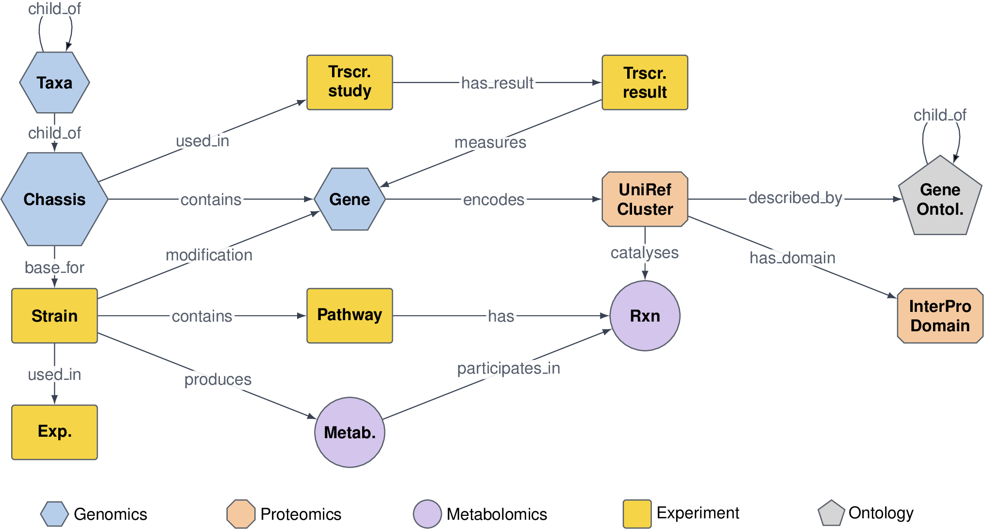
Canopy’s knowledge graph is constructed using BioCypher [13]. We implement ten adapter modules that ingest data from complementary sources and yield nodes and edges in a unified schema.
3.1.0.1 Node types.
The graph contains 13 node types spanning five biological scales: (i) molecular metabolites (InChIKey, SMILES, formula) and reactions; (ii) protein UniRef90 clusters together with their InterPro domains; (iii) genomic genes, chassis organisms, and engineered strains; (iv) functional annotations from the Gene Ontology, metabolic pathways, and NCBI taxonomy; and (v) experimental fermentation runs alongside transcriptomic experiments with per-gene expression measurements.
3.1.0.2 Edge types.
Thirty-four edge types capture relationships across these scales: catalytic associations linking proteins to the reactions they catalyse, pathway membership, genetic modifications (knockouts, knockins, and overexpression edits applied to a strain), functional annotations, ontological structure, experiment tracking, and gene-expression links between transcriptomic measurements and the genes they quantify.
3.1.0.3 Property schema.
Each node property carries a mandatory prefix that declares its role: sys_ for system keys used in deduplication (not exported as features), feat_ for numeric values, text_ for free text routed to the text encoder,
seq_ for amino acid sequences routed to the protein encoder, and smi_ for SMILES routed to the chemical encoder. This dispatch ensures graph construction, embedding, and training share a single source of truth.
3.1.0.4 Data sources.
Molecular data is drawn from MetaNetX [42] and KEGG [43]. Protein data comes from UniRef90 [44] with sequences from UniProt [45] and domain annotations from InterPro [46]. Genomic data includes NCBI gene records [47] and taxonomy [48]. Functional annotations come from the Gene Ontology [49]. Experimental data is sourced from a quality-controlled literature corpus and a proprietary experimental database; transcriptomic data provides per-gene expression linked to experimental conditions.
| Domain | Node type | Count |
|---|---|---|
| Genomics | Taxon | 143 |
| Chassis | 26 | |
| Genomic Gene | 168,913 | |
| Proteomics | UniRef Cluster | 150,914 |
| InterPro Domain | 51,489 | |
| Metabolomics | Metabolite | 1,495,667 |
| Reaction | 83,796 | |
| Experiment | Strain | 6,910 |
| Pathway | 1,872 | |
| Experiment | 4,791 | |
| Transcriptomic | 4,860,266 | |
| Ontology | GO Term (BP/MF/CC) | 38,739 |
| Total | 6,863,526 |
3.2 Multi-Modal Feature Encoding↩︎
Canopy employs three pretrained foundation models as frozen extractors. Protein sequences (seq_) are encoded by ESM-2 [10] (esm2_t33_650M_UR50D) and mean-pooled across residues. Chemical structures (smi_) are encoded by MoLFormer-XL [11]. Biomedical text (text_) is encoded by S-PubMedBERT, applied to GO definitions, gene names and summaries, pathway names, and
experiment descriptions. Numeric features (feat_) are z-score normalised using per-type statistics; categorical integers are one-hot encoded. All features for a node are concatenated into \(\mathbf{x}_{v}\);
per-type input projection handles dimensional heterogeneity.
3.3 Model Architecture↩︎
![Figure 4: Readout. After L stacked HGT layers, JumpingKnowledge max-pools the per-layer representations \{h_v^{(\ell)}\} (combined with a learnable input-residual scale \alpha^{\text{(in)}}_{[\tau]}) and a final per-type LayerNorm produces the encoder output h_v^{\mathrm{out}}.](/article/2607.06224/_pdflatex/zwptmlrd.png "fig:")
![Figure 5: Pretraining objective. Four parallel heads consume the encoder output \{z_v\}_{v\in V}: link prediction (BCE), per-type masked node modelling (MSE), graph-distance regression (MSE), and an Experiment\leftrightarrowExperiment contrastive loss (MSE on cosine similarity). Their weighted sum, using [50] uncertainty weighting, forms the training objective.](/article/2607.06224/_pdflatex/aivpynzu.png "fig:")
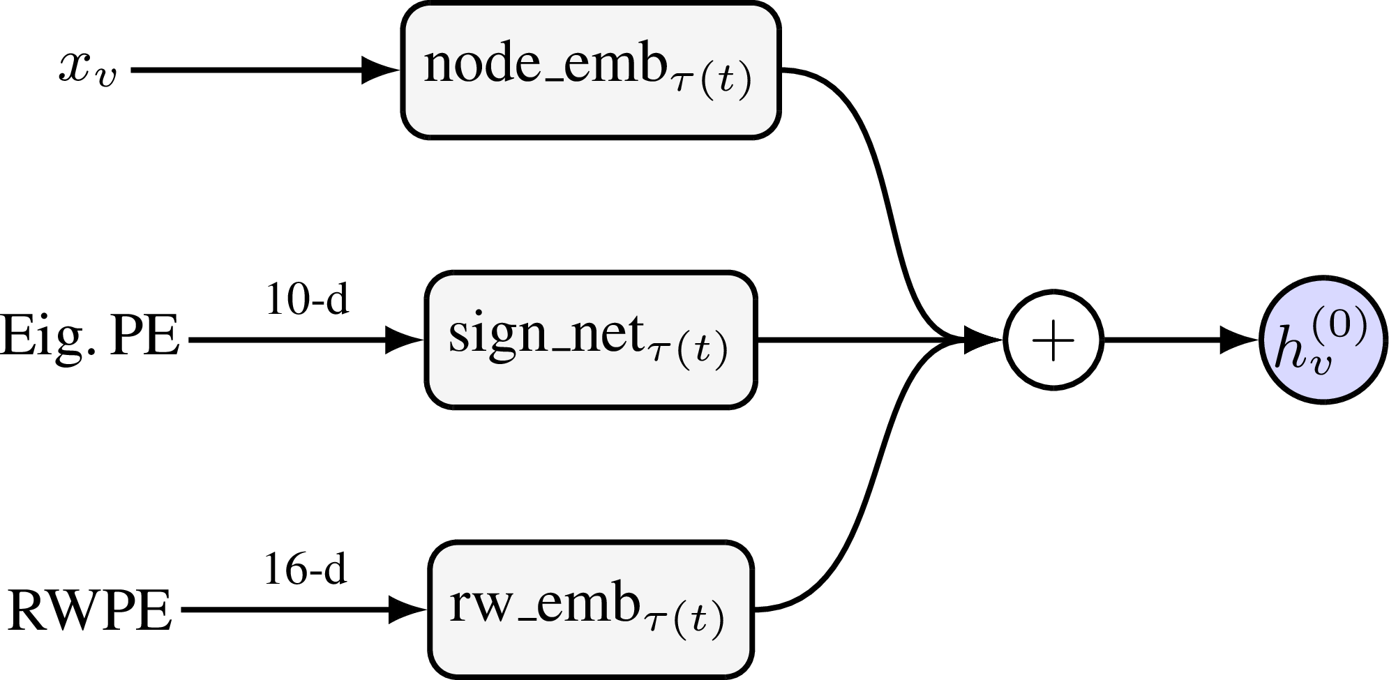
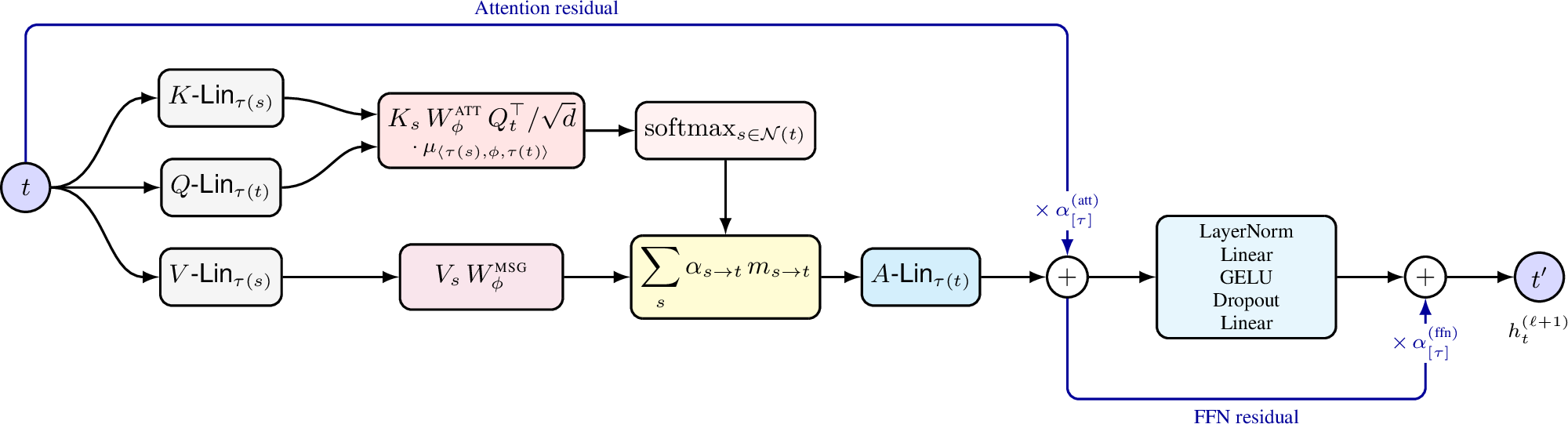
Canopy’s encoder is a Heterogeneous Graph Transformer that processes typed nodes and edges natively, extending HGTConv [8] with several modern components. Figures 2–4 give a schematic overview of the full architecture, including the per-type and per-relation parameterisation that distinguishes HGT from a homogeneous GNN.
3.3.0.1 Input projection.
For each node type \(t\), a learnable linear projection \(\mathbf{W}_{t}\) maps \(\mathbf{x}_{v}\) to a hidden representation of dimension \(d = d_{h} \cdot H\), with \(d_{h}\) the per-head dimension and \(H\) the number of heads.
3.3.0.2 Positional encodings.
We augment node features with two complementary signals. The \(k\) smallest non-trivial Laplacian eigenvectors are computed via randomised SVD and processed through SignNet [36]: \[\text{SignNet}(\mathbf{e}) = \text{MLP}(\mathbf{e}) + \text{MLP}(-\mathbf{e}).\] Random walk structural encodings of length \(\ell\) are computed per subgraph sample and projected per-type. Both encodings are added element-wise to the projected features.
3.3.0.3 Transformer blocks.
The model stacks \(L\) blocks: per-type pre-norm; HGTConv with type-dependent multi-head attention; GELU; a residual connection scaled by a learnable ScaleLayer initialised at 0.1; a per-type FFN with expansion \(r\) and dropout; and a second scaled residual. The small initial scale stabilises training of deep networks by letting the residual stream dominate early. On top of the stack, we apply Jumping Knowledge [38] with max-pooling across all \(L\) layers per type. A virtual node type is added with bidirectional edges to all other nodes, reducing effective graph diameter and providing a shortcut path between otherwise disconnected components. The final representations are layer-normalised.
3.4 Multi-Task Self-Supervised Pretraining↩︎
We pretrain Canopy with four complementary objectives.
3.4.0.1 Hold-out integrity.
The same hash-keyed Experiment-node split used at probe time (Section 4.1) gates every pretraining objective that touches an Experiment node: edges incident to any val/test Experiment are excluded from the
link-prediction label set, masked-node-modelling ignores held-out Experiment rows when sampling its mask, and the contrastive Experiment-clustering loss filters held-out Experiments out of its pair pool before sampling. Held-out Experiment nodes remain in
the message-passing graph so probe-time message passing matches the pretrain-time graph the model was conditioned on; only supervision signal involving their identity, features, or neighbour structure is removed.
3.4.0.2 Link prediction.
Thirty percent of edges are deterministically reserved as supervision labels via an MD5 hash of edge endpoints, ensuring consistent splits across sampling runs (subject to the hold-out filter above). A dot-product predictor scores edges, \(\hat{y}_{uv} = \sigma(\mathbf{z}_{u}^{\top}\mathbf{z}_{v})\), trained with binary cross-entropy. For each edge type we draw negatives at a 1:1 ratio with positives by uniformly sampling type-constrained \((src, dst)\) pairs from the corresponding node pools within the sampled subgraph and rejecting pairs that are already edges.
3.4.0.3 Masked node modelling.
We mask 15% of node features per batch. Per-type linear decoders reconstruct masked features under MSE, which acts as a regulariser against representation collapse.
3.4.0.4 Distance prediction.
For each subgraph, 200 random node pairs are sampled and their shortest-path distances computed via BFS on the undirected graph before virtual-node edges are added (capped at 5 hops); virtual nodes would otherwise collapse the diameter to two and trivialise the target. A distance head (the Hadamard product of source and target embeddings followed by a two-layer MLP) regresses these distances under MSE, supervising pairwise embedding distances against the graph metric.
3.4.0.5 Contrastive experiment-pair loss.
Experiment node embeddings are contrasted within each batch with a target similarity inversely proportional to graph distance, \(s_{ij} = 1 - d_{ij}/d_{\max}\), trained with temperature-scaled cosine similarity (\(\tau {=} 0.07\)).
3.4.0.6 Loss combination.
The four losses are combined via homoscedastic uncertainty weighting [50]. Each task has a learnable log-variance \(\log\sigma_{i}\), and the total loss is \[\mathcal{L} = \sum_{i} \frac{\mathcal{L}_{i}}{2\sigma_{i}^{2}} + \log\sigma_{i}.\] \(\log\sigma_{i}\) is clamped at \(-4.0\) to prevent collapse; tasks with noisier supervision automatically receive lower weight.
3.5 Scalable Subgraph Sampling↩︎
Training on the full graph is infeasible; Canopy uses a Neo4j-backed streaming sampler that constructs mini-batch subgraphs in parallel worker processes and writes each to disk as a PyTorch Geometric [51] HeteroData object. The sampler supports three strategies (simple BFS, batched random walks, and multi-anchor); we use multi-anchor by default. Seeds
are split 50/50 between yield-bearing Experiment nodes (so every probe target appears in some subgraph) and inverse-degree-weighted random nodes (so peripheral nodes are not crowded out by hubs).
For each Experiment seed batch the multi-anchor strategy resolves four BFS anchors: the seed Experiment; its Strain (via uses_strain); parent Taxon plus capped
sibling strains (via belongs_to, capped at 10 per species); and adjacent MetabolicPathways (via has_pathway from the Strain). It also resolves four directed
metapath anchors that walk fixed causal chains the undirected BFS under-covers: Experiment\(\to\)Metabolite (target compound), Pathway\(\to\)Reaction\(\to\)UnirefCluster (pathway enzymes), Strain\(\to\)GenomicGene\(\to\)UnirefCluster (genetic edits to encoded proteins), and the reverse-direction chain Metabolite\(\to\)Reaction\(\to\)UnirefCluster\(\to\)GenomicGene (target enzymes). Each anchor is allocated a fraction of a global node budget \(N_{\max}\) (default 1,000); unused budget from inactive anchors is
proportionally redistributed. Ontological edges (subclass_of, part_of, regulates) and transcriptomic measurement edges are excluded from BFS expansion to prevent
hub-dominated subgraphs but are included in the final subgraph if both endpoints are present. The multi-anchor configuration rebalances the GenomicGene fraction from 78% to 15% and increases Experiment-node coverage roughly \(13\times\) relative to a naive 5-hop BFS. The 30% link-supervision split is computed deterministically via MD5 hashing of (src, rel, dst), so an edge belongs to the same set regardless of which subgraph contains
it; edges incident to held-out Experiment nodes are kept in the message-passing graph but excluded from supervision. Continuous scalar features are z-score normalised per node type, and random-walk positional encodings are added to each subgraph at
materialisation.
3.6 Downstream Tasks↩︎
The prediction target is the measured product titer of each fermentation Experiment: the experimentally reported concentration of the target compound from a physical microbial culture. Titers are drawn from two sources: published metabolic-engineering studies (literature-mined) and unpublished in-house design-build-test-learn runs recorded in our LIMS. After pretraining, we train lightweight probes on frozen experiment-node embeddings: a linear probe and a two-layer MLP probe for titer regression. We report \(R^{2}\), RMSE, and Spearman \(\rho\) for regression, and AUROC and F1 for binary classification (above/below median titer). This protocol isolates representation quality from probe capacity.
4 Experiments↩︎
4.1 Setup↩︎
4.1.0.1 Knowledge graph statistics.
Canopy’s graph comprises 6.9 M nodes across 13 types and 11.2 M edges across 34 typed relations (Table 1, Section 3.1). At training time we additionally materialise reverse edges, self-loops, and virtual-node edges, bringing the per-batch typed-tuple count above 100.
4.1.0.2 Sampling.
We sample 10,000 subgraphs with the multi-anchor expansion (\(k{=}3\), \(N_{\max}{=}1000\)) of Section 3.5. Pretraining uses the deterministic MD5 edge-supervision split described in Section 3.5; the downstream titer probe uses a 5x CV Experiment-node split (Experiment IDs hashed and bucketed) so test experiments are unseen during both pretrain and probe fitting.
4.1.0.3 Model configurations.
We evaluate three scales:
| Config | Hidden | Heads | Layers | FFN | Params |
|---|---|---|---|---|---|
| Demo | 64 | 4 | 6 | 4 | \(\sim\)80M |
| 500M | 128 | 4 | 6 | 4 | \(\sim\)0.5B |
| 3B | 256 | 8 | 12 | 4 | \(\sim\)3B |
4.1.0.4 Training.
AdamW (\(\beta_{1}{=}0.9, \beta_{2}{=}0.999\)) with cosine annealing and linear warmup; bfloat16 mixed precision; FSDP for distributed training across Intel Data Center GPU Max accelerators (Dawn). Gradient clipping at \(\ell_{2}\) norm 1.0. Hyperparameters tuned via a two-tier Optuna [52] sweep: Tier 1 (1,000 trials at 500M, \(\sim\)500 XPU-hours, search over \(h \in \{64,128,192,256\}\), \(L \in \{4,6,8\}\)); Tier 2 (200 trials at 3B, \(\sim\)800 XPU-hours, search narrowed from Tier 1). A single model trains to convergence in 7 XPU-hours at 500M (7 h on one Max GPU) and 160 XPU-hours at 3B (40 h on four); the \(\sim\)500 and \(\sim\)800 XPU-hour budgets above amortise over the 1,000 and 200 median-pruned trials of each tier. Reported parameter counts are for the trainable HGT only: the ESM-2, MoLFormer, and PubMedBERT encoders are frozen and their node features precomputed, so pretraining does not backpropagate through them.
4.1.0.5 Baselines.
Ridge, MLP (two hidden layers, 128\(\to\)64), and XGBoost (500 trees, depth 6) trained directly on the 429-dim raw experiment-condition feature vector (the same input that feeds the Experiment node in the graph), using the identical MD5-hashed train/test split as the Canopy probe. We further compare against graph baselines sharing the same probe and split: a homogeneous GraphSAGE backbone (evaluated both in a vanilla form and with Canopy’s SignNet, Jumping Knowledge, and virtual-node augmentations) and a vanilla HGT backbone without those augmentations. Together with Canopy itself (the HGT backbone with the augmentations), these separate the contribution of the heterogeneous backbone from that of the augmentations.
4.2 Main Results↩︎
| Method | \(R^{2}\uparrow\) | AUROC\(\uparrow\) |
|---|---|---|
| Ridge (raw conditions) | 0.086 | 0.698 |
| XGBoost (raw conditions) | 0.236 | 0.726 |
| MLP (raw conditions) | 0.078 | 0.691 |
| GraphSAGE (vanilla) | 0.241 | 0.713 |
| GraphSAGE \(+\) SN/JK/VN | 0.334 | 0.734 |
| HGT (vanilla) | 0.308 | 0.711 |
| (Demo) | 0.301 | 0.703 |
| (500M) | 0.380 | 0.805 |
| (3B) | 0.413 | 0.820 |
4.3 Ablations↩︎
Unless stated otherwise, ablations are run at the 500M scale defined in Section 4.1 with a 5k-sample budget; the runs in Table 3 use the full 10k-sample budget. Absolute \(R^{2}\) values in the ablations therefore sit below the headline numbers and should be read as relative comparisons.
We ablate the four self-supervised tasks (Table 4), the three architectural augmentations (SignNet PE, Jumping Knowledge, and virtual nodes; Table 5), and network depth (Table 6). For depth, we compare the default \(L{=}6\) architecture against an iso-parameter shallow variant (\(L{=}2\), \(h{=}224\)) at 500M scale. The shallow model reaches a higher peak probe \(R^{2}\), runs \(\sim\)2\(\times\) faster per epoch, and, unlike the deeper variant, does not exhibit probe degradation through 20 epochs. We attribute this to a lower oversmoothing burden once HGTConv attention has enough per-head capacity (\(d_{h}{=}56\)); Jumping Knowledge alone is insufficient at \(L{=}6\) on this graph. We retain the deeper default in the headline configuration: the gap is small (\(\Delta R^{2}{=}0.011\)) and the deeper topology matches the 3B configuration from which we report headline numbers. Mitigations beyond JK and scaled residuals (DropEdge, GraphNorm, or deeper feature fusion) remain unexplored and are a natural next ablation.
| Link | MNM | Dist | Contrast | \(R^{2}\uparrow\) / \(\Delta\)pp | |
|---|---|---|---|---|---|
| ✔ | ✔ | ✔ | ✔ | 0.359 | |
| ✔ | ✔ | ✔ | \(-1.6\) | ||
| ✔ | ✔ | ✔ | \(-0.6\) | ||
| ✔ | ✔ | ✔ | \(-4.7\) | ||
| ✔ | ✔ | ✔ | \(-7.6\) |
| Variant | \(R^{2}\uparrow\) / \(\Delta\)pp |
|---|---|
| Full | 0.359 |
| \(-\) SignNet PE | \(-2.7\) |
| \(-\) JK aggregation | \(-3.5\) |
| \(-\) Virtual nodes | \(-10.3\) |
| \(-\) All three | \(-11.1\) |
| Variant | \(R^{2}\uparrow\) / \(\Delta\)pp | AUROC / \(\Delta\)pp |
|---|---|---|
| \(L{=}2,\,h{=}224\) (shallow) | 0.3703 | 0.7881 |
| \(L{=}6,\,h{=}128\) (deep) | \(-1.0\) | \(-1.1\) |
4.3.0.1 Task weighting.
The four pretraining losses operate on very different scales: BCE for link prediction, MSE for masked-node and distance, and contrastive cosine for experiment pairs. Under flat (equal) weighting the highest-scale loss dominates the gradient and the probe collapses: removing the learned weighting drops \(R^{2}\) by \(9.18\) (\(\Delta R^{2}{=}{-}9.18\) relative to the learned scheme), well below the constant-mean predictor (Table 7). The homoscedastic uncertainty scheme of [50] attains \(R^{2}{=}0.359\). The learned \(\log\sigma_{i}\) values converge to per-task scales that balance gradient contributions automatically and adapt as the relative difficulty of each task shifts during training, removing the manual sweep over fixed per-task weights that would otherwise be needed.
| Weighting | \(R^{2}\uparrow\) | \(\Delta R^{2}\) |
|---|---|---|
| Learned (Kendall) | 0.359 | — |
| Flat (equal) | — | \(-9.18\) |
5 Discussion↩︎
Each of the four pretraining objectives contributes (Table 4), with no single task dominating. Learned uncertainty weighting (Table 7) eliminates manual loss balancing and adapts as training progresses.
The 3B model improves \(R^{2}\) from 0.380 to 0.413 over the 500M model, a modest gain relative to the 6\(\times\) parameter increase. With 4,791 total literature-mined fermentation
records, the regime is likely data-bound rather than capacity-bound at this scale; substantiating scaling claims will require more experimental data, particularly across the long tail of compounds and organisms. In deployment, titer prediction is used to
rank candidate designs for the wet lab rather than to replace measurement; in this triage setting the meaningful gain is in regression, from the best tabular baseline (\(R^{2}{=}0.24\)) to Canopy’s cross-organism representation (\(R^{2}{=}0.41\)). We report AUROC for completeness but read it with caution: fermentation volume (feat_volume) correlates with titer (Pearson
\(0.15\)) and on its own separates above/below-median titer at AUROC \(0.65\), so the binary task is partly trivialised and all methods sit in a narrow AUROC band regardless of regression
skill. Because each fermentation costs weeks of bench time, even a modest improvement in how designs are ranked can reduce the number of physical builds per successful design, though we do not yet quantify this end-to-end.
5.0.0.1 Limitations.
First, experimental data is sparse relative to the KG, with uneven distribution across compounds and organisms. Second, the model is predictive rather than mechanistic; attention analysis offers some interpretability but does not replace mechanistic modelling. Third, our baselines do not include a graph-free pooled-encoder control, e.g., concatenating frozen ESM-2 and MoLFormer embeddings of a strain’s genes and target compound and applying an MLP; such a probe would isolate the contribution of graph structure from the underlying foundation-model encoders and is a planned ablation. Fourth, release scope is constrained for this submission: the 4,791-experiment literature-mined benchmark and its split files will be released in a forthcoming publication, while the in-house LIMS records and trained model weights are not released with this workshop paper, with an archival release of the full pipeline planned to accompany a later journal submission. Fifth, we do not yet isolate the contribution of individual data sources. A node-type feature-masking ablation, which zeros proteomic (UniRef/InterPro), genomic, or transcriptomic features at probe time, would reveal which modalities are influential versus redundant. A per-fold check would test whether the experiment-level split induces feature-distribution shift. Both are planned and inform the data-expansion priorities below.
5.0.0.2 Future work.
Several extensions are already underway. On the representation side, we are scaling node features with larger and more sophisticated embedding models, ingesting orders of magnitude more protein sequences, and adding predicted protein structures as a complementary modality. On the data side, we are expanding the KG with DNA parts (promoters, RBSs, terminators, CDS variants) and metagenomic sequences from environmental and engineered communities, broadening coverage well beyond the current cultured-organism backbone. On the application side, the same frozen embeddings are being extended from titer prediction to chassis selection and de novo pathway design, both of which reuse Canopy’s heterogeneous representation but condition on different query node types. Substantiating the “foundation model” framing also requires breadth in downstream evaluation; beyond titer prediction, we plan probes on chassis selection, gene essentiality, reaction prediction, and cross-organism transfer (e.g., pretraining on E. coli experiments and evaluating on yeast) to test whether the same frozen embeddings transfer across distinct metabolic-engineering tasks. Finally, we are pairing the learned representation with generative strain-design pipelines: a flow-matching model conditioned on Canopy embeddings proposes candidate multi-gene interventions, which are then scored by the frozen titer probe inside a Bayesian-optimisation loop, turning the predictive oracle into a closed-loop generative design system.
5.0.0.3 Broader impact.
Accelerating strain design supports a shift from petrochemical to fermentative production of chemicals, fuels, and therapeutics.
6 Conclusion↩︎
Frozen Canopy embeddings outperform tabular and homogeneous graph baselines on titer prediction, providing a cross-organism representation that can be reused as the conditioning substrate for downstream generative strain-design pipelines.
Impact Statement↩︎
This paper presents work whose goal is to advance the field of machine learning for biological design. There are many potential societal consequences of our work, including positive impact through greener bioproduction.
Acknowledgements↩︎
The authors acknowledge the use of resources provided by the Dawn National AI Research Resource (AIRR). Dawn is operated by the University of Cambridge and is funded by the UK Government’s Department for Science, Innovation and Technology (DSIT) via UK Research and Innovation, the Science and Technology Facilities Council [ST/Z000890/1], Dell Technologies and Intel.
7 Knowledge graph construction details↩︎
Canopy’s graph is assembled with BioCypher [13], which separates
what the graph contains from how it is collected. A single declarative schema (YAML, keyed by Biolink-aligned node and edge types) fixes the allowed types, their identifier namespaces, and their property contracts. Ten adapter modules
each emit typed node and edge streams against that schema; BioCypher rejects labels that are not declared, collapses sub-classes onto the declared parent type, and writes neo4j-admin-importable CSVs. Adapters can therefore be added, swapped,
or version-pinned without touching graph code, and the same schema drives both build-time validation and downstream sampling. The ten adapters span public reference resources (sequence, structure, pathway, ontology), a literature-mined fermentation corpus,
and one in-house LIMS adapter contributing unpublished DBTL records (Table 8).
| Adapter | Source | Nodes / edges produced |
|---|---|---|
| Genomic | UniProt REST + curated chassis list | Chassis, GenomicGene; ENCODES (Gene\(\to\)UnirefCluster), HAS_GENE (Chassis\(\to\)Gene). |
| UniRef | UniRef90 .tsv, MetaNetX cross-refs | UnirefCluster; CATALYZED_BY (Reaction\(\to\)UnirefCluster), HAS_GO_TERM. |
| InterPro | protein2ipr.dat.gz (bulk) or UniProt batch API | InterProDomain; HAS_DOMAIN (UnirefCluster\(\to\)Domain). |
| Gene Ontology | GO OBO release (obonet) | GOTerm (BP/MF/CC); ontology hierarchy edges (subclass_of, part_of, regulates). |
| MetaNetX | MNXref [42] | Metabolite, Reaction; HAS_PARTICIPANT, HAS_PRODUCT. |
| Taxonomy | NCBI Taxonomy | Taxon; BELONGS_TO (Strain\(\to\)Taxon). |
| Transcriptomic | Public RNA-seq compendia | Transcriptomic measurement nodes; MEASURED_BY_TRANSCRIPTOMIC, DERIVED_FROM_TRANSCRIPTOMIC, USES_STRAIN_TRANSCRIPTOMIC edges. |
| Experimental scrape | Literature-mined fermentation records | Experiment, Strain, MetabolicPathway; USES_STRAIN, HAS_PATHWAY, TARGETS_COMPOUND, MEASURES_COMPOUND, HAS_KNOCKOUT, HAS_KNOCKIN, HAS_OVEREXPRESSION. |
| Pathway enrichment | KEGG REST | enriches MetabolicPathway nodes with KEGG metadata; HAS_STEP (Pathway\(\to\)Reaction). |
| LIMS (in-house) | Internal experiment registry | supplements Experiment / Strain with unpublished DBTL records and the edit-edge types above. |
7.0.0.1 Schema harmonisation.
BioCypher’s ontology layer maps every adapter’s emitted labels to Biolink superclasses. Only types declared in the project schema are retained at build time, and sub-class collapse prevents label fragmentation (e.g.”BiologicalProcess” and
“MolecularFunction” are both rolled up under GOTerm). Edges referencing undeclared node types are dropped before import and logged.
7.0.0.2 Identifier normalisation and deduplication.
Cross-source identifiers follow a fixed precedence: MetaNetX MNX IDs for metabolites and reactions, UniRef90 cluster IDs for proteins, NCBI gene IDs for genes, NCBI Taxonomy IDs for taxa, GO IDs for ontology terms, and InterPro IDs for domains. Organism
names in the literature-mined corpus are normalised through a curated synonym table that maps frequently-confused taxonomic labels (e.g.Pichia pastoris \(\to\) Komagataella phaffii, Clostridium
thermocellum \(\to\) Acetivibrio thermocellus) to the canonical chassis list. Duplicate metabolite and reaction nodes from MetaNetX cross-references are merged on MNX ID; Uniref\(\to\)Reaction and Uniref\(\to\)GOTerm mappings are resolved against the MetaNetX curated reaction model and the GO release pinned at build time. Edges with
malformed or missing endpoints are dropped at adapter time and logged.
7.0.0.3 Build pipeline.
Adapters write CSVs to a staging directory, BioCypher emits the matching neo4j-admin headers and edge files, and the resulting graph is loaded into Neo4j 5 via neo4j-admin import. The final graph contains 6.86 M nodes and
11.2 M schema-typed edges across 13 node types and 34 typed relations (Table 1).
8 Hyperparameter sweep details↩︎
Hyperparameters are selected with a staged Optuna sweep that narrows the search as model scale increases (Section 4.1). Tier 1 explores broadly at the 500M scale on a single XPU; Tier 2 refines around the Tier 1 optimum
at the 3B operating point under FSDP across four XPUs, optionally with gradient checkpointing. All trials optimise the held-out titer probe \(R^{2}\) at its best epoch, and both studies use Optuna’s TPESampler
with median pruning.
Tables 9 and 10 list the Tier 1 and Tier 2 search spaces in full. Trials whose hidden_channels is not divisible by heads are pruned at sample time.
| Parameter | Range / set | Sampling |
|---|---|---|
| Architecture | ||
| hidden_channels | \(\{64, 128, 192, 256\}\) | categorical |
| num_layers | \([2, 8]\) | integer |
| heads | \([2, 8]\) | integer |
| ffn_expansion | \(\{2, 4\}\) | categorical |
| dropout | \([0.05, 0.40]\) | float |
| Optimisation | ||
| lr | \([10^{-4}, 5{\times}10^{-3}]\) | log-uniform |
| weight_decay | \([10^{-4}, 10^{-1}]\) | log-uniform |
| warmup_epochs | \([1, 10]\) | integer |
| cosine_end_offset | \([1, 30]\) | integer |
| batch_size | \(\{8, 16, 32, 64, 128, 256\}\) | categorical |
| accumulate_grad_batches | \(\{1, 2, 4\}\) | categorical |
| Probe geometry | ||
| probe_hidden_dim | \(\{32, 64, 128, 256\}\) | categorical |
| probe_num_layers | \([1, 4]\) | integer |
| probe_dropout | \([0.0, 0.3]\) | float |
| Parameter | Range / set | Sampling |
|---|---|---|
| Architecture | ||
| hidden_channels | \(\{192, 256, 384\}\) | categorical |
| num_layers | \([8, 12]\) | integer |
| heads | \([4, 8]\) | integer |
| ffn_expansion | \(\{2, 4\}\) | categorical |
| dropout | \([0.05, 0.30]\) | float |
| Optimisation | ||
| lr | \([5{\times}10^{-5}, 3{\times}10^{-3}]\) | log-uniform |
| weight_decay | \([10^{-4}, 10^{-1}]\) | log-uniform |
| warmup_epochs | \([2, 10]\) | integer |
| cosine_end_offset | \([1, 15]\) | integer |
| batch_size | \(\{32, 64, 128\}\) | categorical |
| accumulate_grad_batches | \(\{1, 2, 4, 8\}\) | categorical |
The Tier-1 winner combines \(L{=}6\), \(h{=}128\) (matching the 500M row of Table 2) with \(\mathrm{bs}{=}256\), \(\mathrm{lr}{=}2{\times}10^{-3}\), four warmup epochs, a cosine_end_offset of 6, and all four pretraining losses active. This configuration is used for the 500M headline run and seeded the Tier-2 search at 3B
scale.