Chunky Chains: Graph Drawings on Small Screens
July 07, 2026
Abstract
We introduce , a graph drawing style designed for small screens such as smartphones, where vertical scrolling is the dominant means of interaction. A Chunky Chain consists of a vertical chain of chord diagrams, called . Vertices are placed as circular arcs on bucket boundaries, and edges are drawn inside a bucket or through connecting consecutive buckets. Since every bucket contains only a bounded number of vertices, the drawing has bounded width. The combinatorial core is the choice of a . Given a \(c\), the vertices are partitioned into an ordered set of buckets, each of size at most \(c\). Edges whose endpoints lie in the same or in adjacent buckets are . Edges that are “skipping” at least one bucket are , and we draw them only partially. The goal is to minimize the number of long edges.
We present a combinatorial framework for producing high quality Chunky Chains and analyze the complexity of its steps. We develop exact and heuristic algorithms, and experimentally evaluate their effectiveness. Our experiments show that many real-world graphs have good Chunky Chain visualizations. In a case study, we discuss Chunky Chains for graphs with certain temporal features.

1 Introduction↩︎
Smartphone screens are arguably the most common type of screen that displays information nowadays. Due to their limited size, content rarely fits entirely on the screen, requiring users to explore it through zooming, panning, and (vertical) scrolling. In many applications, such as social media feeds, scrolling is the dominant mode of navigation.
Following this trend, graph visualizations with small width (but possibly large height) are natural to consider. Hence, the task (T1) is to visualize graphs on narrow screens in a linear
fashion that promotes vertical scrolling to explore the drawing. To this end, we present . Intuitively, a Chunky Chain is a graph drawing that places vertices on a vertical chain of circles. We call them and draw them as chord diagrams. Adjacent vertices
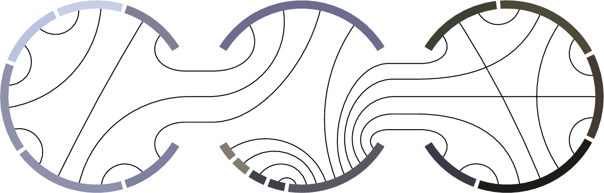
should ideally be assigned to the same or adjacent buckets. See 1 for an example of a Chunky Chain that visualizes the spatial color co-occurrences in Vincent van Gogh’s “Starry Night Over the Rhône” (see 8 for details). Naturally, such a constraint on the aspect ratio benefits the visualization of sequential or weakly branching structures the most. We aim to
(T2) reveal these structures with Chunky Chains. Interestingly, in 1 our algorithm unveils a hidden correlation between the colors as our algorithm apparently ordered the colors from blue, over teal and green, to
ocher.
Problem Statement.
From a combinatorial perspective, we want to find a of a given graph \(G\). A bucket arrangement is a partition of \(V(G)\) into \(k\) buckets \(B_1,\dots,B_k\). Ideally, we want to find a bucket arrangement such that each edge is short. An edge \(\{u,v\}\) with \(u\in B_i, v\in B_j\) is , if we have \(|i-j|<2\). The smallest \(\max_i |B_i|\) of such a bucket arrangement is a graph parameter known as in the literature.
Problem 1 (Bucketwidth). Given a graph \(G\), find a bucket arrangement of \(G\) of minimum width that consists of only short edges.
Unfortunately, the width of a screen (and potential space for labels) restricts the number of vertices that can be assigned to a bucket. This requires an additional input parameter that limits the of each bucket. Consequently, it may not be possible that every edge is short. We call edges in a given bucket arrangement for which this fails . Since we want to avoid long edges, we obtain the following combinatorial core of Chunky Chains.
Problem 2 (Bucket Integrity). Given a graph \(G\) and a capacity \(c\in\mathbb{N}\), find a bucket arrangement of \(G\) with width at most \(c\) and the minimum number of long edges.
Note that this problem can be viewed as an edge-deletion distance problem to the decision version of Bucketwidth. In the following, we set \(n=|V(G)|\) and \(m=|E(G)|\) if the graph \(G\) is clear from the context, and we write \(N(v)\) for the neighborhood of a vertex \(v\). For a given bucket arrangement, \(\mathcal{L}\) denotes the set of long edges, and we set \(\ell = |\mathcal{L}|\).
Related Work.
While an aspect ratio (width/height) close to 1 is often pursued in graph drawing, technical and environmental constraints can push towards an unbalanced aspect ratio even apart from digital screens. A historic example is the Tabula Peutingeriana [1], a Late Antique Roman road map on an enormous parchment scroll measuring 33 cm in height and 680 cm in length (a stunning aspect ratio of approximately 0.05).
Our design is inspired by ChordLink [2], [3], a hybrid drawing style combining node-link and chord diagrams [4]. ChordLink was introduced by Angori, Didimo, Montecchiani, Pagliuca, and Tappini. While ChordLink integrates into an interactive workflow and tries to keep the layout stable, our framework is designed to create a layout from scratch without user input. Kindermann, Sauer, and Wolff [5] proved that several steps of the ChordLink pipeline are -hard to compute. In a user study with 82 participants, several tasks related to structural properties of the network could be performed more accurate (albeit slower) with ChordLink compared to classical node-link diagrams [6], [7]. The drawings by Six and Tollis [8] can be considered a precursor of ChordLink. They use circular layouts instead of chord diagrams.
Crossing reduction in circular layouts (or the equivalent task of reducing crossings between chords in chord diagrams) has been proven to be -hard by Masuda, Kashiwabara, Nakajima, and Fujisawa [9]. Among many others, Klawitter, Mchedlidze, and Nöllenburg [10] presented heuristics for this problem. We built our heuristic for crossing minimization in Chunky Chains (see 4.2) upon their algorithm. Our design of gate nodes, that allow us to avoid the node duplication performed by ChordLink, is inspired by Baur and Brandes’ multi-circular layout [11]. We draw long edges only partially. See [12] for an overview of partial edge drawings.
We are not the first ones to consider graph drawings on smartphone screens. Da Lozzo, Di Battista, and Ingrassia [13], [14] draw the neighborhood of a user-selected focus vertex and explore smartphone-specific interaction methods. Aulbach, Fink, Schuhmann, and Wolff [15] select a maximum-weight subgraph that can be drawn inside the restricted area of a small screen. For planar graphs, only polynomially bounded coordinate-precision is required to draw it entirely inside a fixed polygon [16], [17]. Another way to tackle the issue of small screens is to limit the aspect ratio. Efficient algorithms are known for binary trees [18], [19]. Heuristic methods have been presented for layered drawings [20], [21] and, very recently, orthogonal layouts [22]. In principle, all linear layouts can be drawn with bounded width (depending on the edge geometry). See [23] for an overview of linear layouts.
On the combinatorial side, Bucket Integrity is a generalization of Bucketwidth (see 1 2). Bucketwidth has mainly been investigated as a means to obtain approximation results for Bandwidth since the bucketwidth of a graph \(G\) is within a factor of 2 of the bandwidth of \(G\) [24]–[29]. Aside from applications for Bandwidth, Bucketwidth is related to several width measures in parameterized complexity theory. In particular, it is the pendant to tree-partition width [30]–[32] in the same way as pathwidth is the pendant to treewidth. Tree-partition width is defined analogously to Bucketwidth but the quotient graph of the partition is allowed to be a tree. Several intractable problems for treewidth become tractable for tree-partition width [33]. Partition width measures are also important in graph drawing. For example, for drawing graphs with few slopes [34], computing straight line 3d grid graphs with small volume [35], [36], and bounding several notions of crossing numbers [37].
Contribution and Organization.
We introduce Chunky Chains, a drawing style that aims to visualize graphs on narrow screens. We start with a definition and quality metrics in 2. We investigate theoretical aspects of the underlying combinatorial problem and practical approaches, culminating in a pipeline for drawing Chunky Chains. In particular, we analyze the (parameterized) complexity of Bucket Integrity and propose an -algorithm with respect to the vertex cover number, and an exact algorithm which is tight under the exponential time hypothesis. Furthermore, we consider a tractable variant of Bucket Integrity called Ordered Bucket Integrity motivated by heuristics (see 3).
The pipeline for drawing Chunky Chains consists of three steps; see 4. Firstly, vertices are assigned to buckets. Here we devise an ILP and heuristics. Secondly, we compute an ordering of the vertices within the buckets to minimize crossings. Finally, we consider geometric aspects of drawing Chunky Chains. We conclude with a case study (5), an experimental evaluation (6), and open questions (7).
2 The Chunky Chain Method↩︎
We outline the functional requirements of a Chunky Chain, describe its structural design, and identify the key metrics that quantify its effectiveness.
Requirements.
Because we are targeting smartphone screens, we do not want to burden our users with horizontal scrolling [tkey:T1]. Therefore, we require that our drawings have (R1) bounded width. Precisely, we require it to be polynomially bounded in some user-defined parameter. Furthermore, for a comprehensible drawing, we require (R2) vertices to be unobstructed, unambiguous, and (optionally) labeled. It is difficult to follow long edges, especially if they make many turns. Therefore, we require (R3) constant edge complexity. Our edges are sequences of segments where each segment is either a straight line segment, a circular arc, or a cubic Bézier curve. We require edges to be comprised of a constant
number of segments.
Methodology.
A Chunky Chain is a series of chord diagrams. We call the set of vertices that is drawn as one chord diagram a . In a chord diagram every vertex is represented by a circular arc. All vertices of a bucket lie on a circle and each circle has the same radius. We bound the width of the chord diagrams (and therefore the width of the drawing) with an input parameter \(c\) which limits the size of each bucket [tkey:R1]. Vertex labels can be attached to each vertex at the boundary of the diagram [tkey:R2] where they do not obstruct other parts of the drawing. An edge between two vertices in the same bucket is represented by a curve inside the circle that connects the two arcs of the vertices. Edges between two vertices of adjacent buckets are routed through two , special vertices (that we usually do not draw) at the top and bottom of each chord diagram. Long edges are partially drawn using two arrows starting at the incident vertices, respectively, and a corresponding pair of labels. See 2 for illustration (rotated by \(90^\circ\) to better utilize the space on the page) and 5 for a real-world example.
Quality Metrics.
The Chunky Chains method naturally leads to some quality metrics. First and foremost, (M1) the number of fully drawn edges (i.e., the number of short edges) should be as high as possible. We
also prefer (M2) few gate transitions in order to reduce the risk of loosing track in crowded areas and because of the limited space in gate nodes.
Many common graph drawing metrics apply to Chunky Chains. We can equivalently state [tkey:M2] as preferring shorter edges because edges that stay inside a bucket are shorter than
those connecting adjacent buckets (and shorter edges are easier to follow and often mean less scrolling). Furthermore, we want to keep (M3) the number of crossings in our drawings low.
3 Combinatorial Results↩︎
We investigate the (parameterized) complexity of Bucket Integrity and derive useful characteristics of bucket arrangements, starting with an upper bound on the number of buckets for optimal bucket arrangements. This bound is of interest because it limits the vertical extent of a Chunky Chain, and thus the amount of scrolling required in the worst case. Also, this upper bound is a crucial ingredient in our integer linear programming (ILP) formulation (see 4.1). Later we consider a variant of Bucket Integrity called Ordered Bucket Integrity which turns out to be useful for heuristic algorithms.
Lemma 1. Let \((G, c)\) be an instance of Bucket Integrity. Any optimal bucket arrangement of \(G\) uses at most \(\lfloor\frac{3n}{2c}\rfloor\) many buckets and \(\lfloor\frac{3n}{2(c+2)}\rfloor\) are sometimes required.
Proof. We first show that \(\lfloor\frac{3n}{2c}\rfloor\) is indeed an upper bound on the number of buckets. Towards a contradiction, suppose there is a graph \(G\) and a capacity \(c\) where every optimal solution requires at least \(a := \lfloor\frac{3n}{2c}\rfloor +1\) many buckets. Subsequently, every solution has at least \(a/3 \ge n/2c\) many (non-overlapping) triplets of consecutive buckets. Thus, the average number of vertices in each triplet is at most \(2c\), implying that there must be a triplet with at most \(2c\) vertices. This triplet can be compressed into two buckets by removing the middle bucket (and distributing the vertices in the middle bucket) which cannot introduce any long edges. This is a contradiction to the assumption that every optimal solution requires at least \(a\) buckets.
For any capacity \(c\), there exists a family \(\mathcal{G}_{c}\) of graphs for which every optimal solution requires \(\Lambda' = \lfloor\frac{3n}{2(c+2)}\rfloor\) many buckets. For a given capacity \(c\) and a natural number \(\Lambda' > 2\), the graph \(G_{\Lambda'} \in \mathcal{G}_{c}\) consists of \({\Lambda'}\) cliques \(C_1, \dots, C_{\Lambda'}\) of size \(\lfloor 2c/3 \rfloor+ 1\), where for each \(1\leq i \leq {\Lambda'}-1\), the induced subgraph of \(C_i \cup C_{i+1}\) is a complete graph.
Obviously, \(\Lambda'\) many buckets suffice to construct a solution without any long edge. Suppose there exists a solution where the vertices of a clique \(C_i\), \(2 \leq i \leq \Lambda'-1\), are contained in two consecutive buckets, i.e., there are two vertices \(u, v\) of \(C_i\) that are in different buckets \(B_u\), \(B_v\). These vertices have \(2c + 1\) many neighbors in common (other than themselves). Consequently, at least one neighbor is neither in \(B_u\) nor in \(B_v\), resulting in a long edge. Therefore, each \(C_i\) with \(2\leq i \leq \Lambda'-1\) is contained in one bucket. Technically, \(C_1\), \(C_{\Lambda'}\) can be distributed among two consecutive buckets, respectively. However, there exists at least one vertex of \(C_1\) (\(C_{\Lambda'}\) respectively) that is in a bucket that only contains vertices of \(C_1\) (\(C_{\Lambda'}\) respectively). This follows from the fact that in a bucket that contains some clique \(C_i\), the entire clique \(C_i\) must be in this bucket, the clique \(C_1\) (\(C_{\Lambda'}\) respectively) can only be contained in at most two consecutive buckets, and two buckets cannot contain three cliques. Therefore, the number of buckets is at least \(\Lambda'\). ◻
A (Parameterized) Complexity Overview.
Since Bucket Integrity is a generalization of Bucketwidth, we know that Bucket Integrity is -hard due to the -hardness of Bucketwidth. We show that there is no subexponential time algorithm for Bucket Integrity and propose an exact algorithm that matches this single-exponential lower bound.
Lemma 2. Assuming the Exponential Time Hypothesis, Bucket Integrity cannot be solved in \(2^{o(n)}\cdot n^{O(1)}\) time.
Proof. Note that we can solve Hamiltonian Path using Bucket Integrity by setting the capacity to 1. Then, a given graph \(G\) has a Hamiltonian path if and only if the number of long edges is \(|E(G)| - n + 1\). However, Hamiltonian Path cannot be solved in \(2^{o(n)}\cdot n^{O(1)}\) unless the Exponential Time Hypothesis fails [38]. ◻
Note that this lower bound can be reached by a dynamic program that leverages the path structure of a Bucket Integrity solution.
Theorem 1. Let \((G, c)\) be an instance of Bucket Integrity. An optimal solution of \((G, c)\) can be computed in \(O(5.6569^n)\) time and \(O(2.8285^n)\) space.
Proof. We use dynamic programming over subsets of vertices of \(G\). Let \(L\) be a subset of \(V(G)\) of size at most \(n/2\), and let \(G[L]\) be the subgraph of \(G\) induced by \(L\). We define a table entry \(D[L, B]\) to be the minimum number of long edges for a bucket arrangement of \(G[L]\), in which \(B \subseteq L\) is the rightmost bucket.
We compute the table \(D\) by using the following base cases. We set \(D[B, B] = 0\) for all \(B \subseteq V\) with \(|B| \leq c\). This corresponds to the case where all vertices are in a single bucket. Additionally, we set \(D[L, B] = \infty\) for all \(|B| > c\) since this constitutes an invalid bucket arrangement for any \(L\).
For the recursive case, let \(E[U, W]\) denote the set of edges in \(G\) with one endpoint in \(U \subseteq V(G)\) and one endpoint in \(W\subseteq V(G)\). Then, for some \(B' \subseteq L \setminus B\) that represents the unique adjacent bucket of \(B\), the set \(E[B, L\setminus (B'\cup B)]\) describes all long edges that go over \(B'\) in \(G[L]\) in any bucket arrangement, where \(B'\) and \(B\) are the last two buckets. This allows us to compute \(D[L, B]\) as follows. \[\begin{align} D[L, B] = \min_{B' \subseteq L\setminus B}\{D[L\setminus B, B'] + |E[B, L\setminus (B'\cup B)]|\}. \end{align}\]
Note that in any (optimal) bucket arrangement, there is a bucket \(M\) whose removal results in two halves that each have at most \(n/2\) vertices. Based on this observation and \(D\) we compute an optimal solution as follows.
We iterate over all possible subsets \(M \subseteq V(G)\) of size at most \(c\). For a given set \(M\), we test all possible subsets \(L\) of vertices that lie to the left of \(M\); a choice of \(L\) determines the subset of vertices \(R\) that lies to the right of \(M\). Hence, we can calculate the minimum number of long edges for a fixed \(L\), \(M\), and \(R\) by \[\begin{align} |E[L, R]| + \min_{B \subseteq L}\{D[L, B] + |E[L\setminus B, M]|\} + \min_{B \subseteq R}\{D[R, B] + |E[R\setminus B, M]|\}. \end{align}\] This corresponds to iterating over two rows in \(D\) (one for \(L\) and one for \(R\)). Therefore, we get a total runtime of \(O^*(4^n)\) for the computation of \(D\), since there are \(O(2^n \cdot 2^{n/2})\) entries, and we need \(O^*(2^{n/2})\) time to compute one entry. We consider \(O(4^n)\) combinations of \(M\) and \(L\). For a combination \((M, L)\) we compute the minimum number of long edges of this combination in \(O^*(2^{n/2})\) time. Hence, we get a total runtime of \(O^*(4^n) + O^*((4\sqrt{2})^n)\) with a space consumption of \(O((2\sqrt{2})^n\log n)\). ◻
Due to the connection between Bucket Integrity and Bucketwidth, we can consult known results of Bucketwidth to derive several observations about the (parameterized) complexity of Bucket Integrity.
Bucket Integrity is
(i) -hard even on graphs with bounded pathwidth (and therefore bounded treewidth),
(ii) -hard even if the number of long edges is bounded,
(iii) -hard even if the maximum degree of the input graph is bounded,
(iv) -hard with respect to the capacity \(c\),
(v) inapproximable within any constant factor unless \(\P = \NP\).
Observations ([np-hard-pw-tw]) and ([inapprox]) follow from the fact that Bandwidth cannot be approximated within any constant even for caterpillars of hairlength 3 unless \(\P = \NP\) and an observation that Bucketwidth and Bandwidth are within a factor of 2 from each other [25]. Observation ([np-hard-l]) is a direct consequence of the fact that Bucketwidth is -hard, and observation ([np-hard-max-degree]) and ([np-hard-c]) follow from the proof in 2 since the proof uses \(c=1\) and Hamiltonian Path is -hard even on graphs with bounded degree [39].
Even though Bucket Integrity is -hard for graphs with bounded pathwidth, we can still derive an upper bound on the pathwidth of the input graph in terms of the capacity and the number of long edges. Therefore, a solution of Bucket Integrity with few long edges and small capacity implies that the input graph has small pathwidth.
Lemma 3. Let \((G, c)\) be an instance of Bucket Integrity and let \(\ell\) be the minimum number of long edges required in any bucket arrangement of \(G\). Then, \(\operatorname{pw}(G) \leq 2c + \ell - 1\).
Proof. Take a solution with \(\ell\) long edges. For two adjacent buckets, create an intermediate bucket that contains the vertices of every edge between vertices of the adjacent buckets. This intermediate bucket contains at most \(2c\) vertices. For every long edge \(\{u, v\} \in E(G)\), where \(u\) is in bucket \(i\) and \(v\) is in bucket \(j\) \((i < j)\), choose either \(u\) or \(v\) and add it into every bucket \(k\) for \(i < k < j\). The buckets form a valid path decomposition and every bucket has size at most \(2c + \ell\). ◻
It would be desirable to derive an upper bound on a function of \(c\) and \(\ell\) that only depends on structural graph parameters, but not on the input size. Unfortunately, for any combination of parameters that are invariant under (graph) duplication such as \(\operatorname{pw}(G)\) or the maximum degree of \(G\), this is impossible if \(\ell > 0\). To see this, suppose a graph \(G\) and a given capacity \(c\) requires \(\ell\) long edges. Then, we can simply take \(k\) copies of \(G\). As a consequence, the number of long edges increases to \(k\cdot\ell\) but the graph parameters do not change.
On the positive side, Bucket Integrity becomes fixed-parameter tractable when parameterized by the vertex cover number of the input graph.
Theorem 2. Let \((G, c)\) be an instance of Bucket Integrity and let \(C\) be a minimum vertex cover of \(G\). An optimal solution of \((G, c)\) can be computed in \(2^{O(|C|\log|C|)}\cdot n^{O(1)}\) time.
Proof. Let \(I = V(G) \setminus C\) be the remaining vertices in \(G\). Note that \(I\) is an independent set, since \(C\) is a vertex cover. The general idea of the algorithm is the following. Firstly, we guess a bucket arrangement of the vertices in \(C\) in -time. Then, for a fixed bucket arrangement of \(C\), we optimally place the vertices of \(I\) into buckets in polynomial time by reducing this subproblem to a matching problem. Out of all bucket arrangements, we choose the one with the fewest long edges.
To guess the optimal bucket arrangement of the vertex cover in -time we show that a bucket arrangement of \(C\) with \(k = 3|C|\) buckets suffices to consider. Indeed, if we place three (or more) buckets between buckets that contain vertices in \(C\), then every vertex \(v\) in \(I\) that is not placed immediately adjacent to a bucket that contains a vertex in \(C\) will only be incident to long edges due to the independence of \(I\). Thus, we can alternatively add such vertices in a post-processing step using additional buckets that are placed at the end of the arrangement. As a consequence, we only need to consider buckets that contain vertices in \(C\) or are immediately adjacent to a bucket with vertices in \(C\), implying that \(3|C|\) buckets suffice.
Now, assume that a bucket arrangement of \(C\) is fixed, i.e., we have \(B_1, \dots, B_{3|C|}\) buckets where \(C\) is divided into buckets \(B_1, \dots, B_{3|C|}\) conforming to the capacity constraints with \(c - |B_i|\) free each in which we can place vertices in \(I\). We construct an auxiliary bipartite weighted graph \(H\) whose vertices comprise the vertices in \(I\), every free slot of the bucket arrangement, and a dummy slot-vertex \(s_{v}^\mathrm{r}\) for every vertex in \(I\). Edges in \(H\) are between slots and vertices in \(I\). For each edge \(\{v, s\}\), where \(v \in I\) and \(s\) is a free slot, we define the weight \(w(\{v, s\})\) to be the number of long edges incident to \(v\) if we place \(v\) in slot \(s\). Since \(N(v)\) is a subset of \(C\), this number is independent of the placement of other vertices in \(I\). If \(s = s_{v}^\mathrm{r}\) we set \(w(\{v, s_v^\mathrm{r}\}) = |N(v)|\). An optimal placement of the vertices in \(I\) given the fixed bucket arrangement is now equivalent to finding a minimum weight matching in \(H\) which can be done in polynomial time.
In total, we guess \(3|C|^{|C|} \in 2^{{O}(|C|\log|C|)}\) many bucket arrangements. For each bucket arrangement we need polynomial time to determine the optimal number of long edges for this bucket arrangement. Therefore, Bucket Integrity is with respect to the vertex cover number. ◻
Ordered Bucket Integrity.
We consider a variant of Bucket Integrity that is solvable in polynomial time. When designing heuristics for Bucket Integrity, this variant proved to be effective (see [ssec:arrangement] [sec:experiments]).
Problem 3 (Ordered Bucket Integrity). Let \(\sigma = \langle v_1,\dots,v_n\rangle\) be an ordered set of vertices in a graph \(G\) and let \(c\in\mathbb{N}\). A bucket arrangement\(B_1, \dots, B_k\) of \(G\) is called (with respect to \(\sigma\)) if \(i < j\) implies \(p \leq q\) for every \(v_i \in B_p, v_j \in B_q\).
Even though it would be tempting to simply divide the ordering into chunks of size \(c\), this approach is not optimal (in fact, there are instances in which many buckets are not completely filled). However, we can still compute an optimal solution in polynomial time.
Theorem 3. Ordered Bucket Integrity can be solved in \(O(nc^2)\) time and space.
Proof. We use dynamic programming. Let \(D[i, d, f]\) be the minimum number of long edges of a bucket arrangement of the induced subgraph of the first \(i\) vertices in \(\sigma\) where the last two buckets \(B_{k-1}\), \(B_k\) have a size of \(|B_{k-1}| = d\) and \(|B_{k}| = f\). By definition, an optimal solution can be found by computing \(\min_{1\leq d,f \leq c} D[n, d, f]\).
We use the base case \(D[0, d, f] = 0\) for all \(1 \leq d, f\leq c\). For \(i \geq 1\), we do the following. Since we compute an ordered bucket arrangement, \(v_i\) has to be in the last bucket of any bucket arrangement of the first \(i\) vertices. Thus, any edge \(\{v_i, v_j\}\) in \(G[\{v_1, \dots, v_i\}]\) is a long edge in any ordered bucket arrangement whose last two buckets have sizes \(d\) and \(f\), respectively, if \(j\) is at most \(i-d-f\). Therefore, we can compute the recursive case for \(i > 0\) and \(1 \leq d, f\leq c\) as follows. \[\begin{align} D[i, d, f] = \begin{cases} D[i-1, d, f-1] + |\{\{v_i, v_j\} \in E(G) \mid j \leq i-d-f\}| & \text{if } f > 1, \\ \displaystyle\min_{1 \leq d' \leq c}\{D[i-1, d', d] + |\{\{v_i, v_j\} \in E(G) \mid j < i-d\}|\} &\text{else.} \end{cases} \end{align}\] Since every edge \(\{v_i, v_j\}\) is always a long edge if \(|j-i| > 2c\), we can remove these edges in a preprocessing step. As a consequence, \(|N(v)| \in O(c)\). Now, to process a vertex \(v_i\) for cases with \(f > 1\), we order (increasingly) the neighbors \(N(v_i) \cap \{v_1, \dots, v_i\}\) of \(v_i\) by their indices in \(\sigma\) which can easily be done in \(O(c\log c)\) time. Let \(N_\sigma(v_i)\) be this order. We fill the two-dimensional table \(D[i, d, f]\) of \(v_i\), by iterating over pairs \(d, f\) whose sum \(d+f\) correspond to increasing values in the range \(\{1, \dots, 2c\}\). In other words, we fill the table along the diagonals of \(D[i, d, f]\) from top-left to bottom-right. Since we fill the table for increasing values of \(d+f\), we can maintain the current number of short edges incident to \(v_i\) by moving an index \(x\) through the sorted neighborhood \(N_\sigma(v_i)\) from right to left while iterating over increasing the values of \(d+f\). Initially, \(x=|N_\sigma(v)|\) and points to the rightmost neighbor left to \(v_i\) in \(\sigma\). For each pair \(d, f\) we test if the index of the vertex \(v_j\), that \(x\) currently points to, is at least \(i-(d+f)\). If this is the case, \(v_j\) is in one of the last two buckets which makes \(\{v_i, v_j\}\) a short edge, and we increment \(x\). In this way, \(|N_\sigma(v_i)| - x\) corresponds to the number of long edges incident to \(v_i\) for the current choice of \(d\) and \(f\). There are at most \(O(nc)\) many entries where \(f=1\). For each of these entries we can easily compute its value in \(O(c)\) time. Consequently, we can process a vertex \(v_i\) in \(O(c^2)\) time, yielding a total runtime of \(O(nc^2)\). We can retrieve an optimal bucket arrangement from the table \(D\) using standard techniques. ◻
4 Pipeline↩︎
We use a three-phase pipeline to compute Chunky Chain visualizations. The input is a graph \(G\) and a capacity \(c\in\mathbb{N}\). Firstly, we compute a bucket arrangement for \(G\) that has width at most \(c\) and few long edges (see 4.1). Secondly, we order the vertices in each bucket such that few edges cross (see 4.2). Thirdly, we calculate the geometry for the actual drawing (see 4.3).
4.1 Computing Bucket Arrangements↩︎
The basic structure of a Chunky Chain is determined by a bucket arrangement. The input parameter \(c\) limits the width of our drawing [tkey:R1] while, for drawing quality, we seek to produce as few long edges as possible [tkey:M1]. Note that graph parameters can already hint at the number of long edges. If \(c \leq \lceil(\Delta+1)/3\rceil\), where \(\Delta\) is the maximum degree of any vertex in \(V(G)\), any bucket arrangement of width \(c\) has long edges. When \(G\) has bandwidth \(b_G\) and \(c \geq b_G\), then a bucket arrangement with width \(c\) exists that has only short edges.
To compute a bucket arrangement, we present an integer linear programming (ILP) formulation for Bucket Integrity and a heuristic that is faster on large graphs. We use \([n]\) as a shorthand for \(\{1, \dots, n\}\).
Integer Linear Programming Formulation for Bucket Integrity.
Based on the definition of 2, we can formulate an intuitive ILP that minimizes the number of long edges, using binary variables representing a vertex to bucket assignment, and binary variables for each edge representing whether the edge is long or not. The upper bound \(\Lambda\) on the number of buckets that 1 provides can be used to limit the number of variables used. The weakness of this formulation is that we need \(O(\Lambda^2)\) constraints for every edge in order to model a long edge. Alternatively, we can maximize the number of short edges which yields a more compact formulation. More precisely, we use the following variables.
\(x_{i,v}\) for \(v\in V(G)\), \(i\in[\Lambda]\), equals \(1\) if \(v\) is in bucket \(i\), \(0\) otherwise.
\(y_{i,u,v}\) for \(\{u,v\}\in E(G)\) and \(i\in[\Lambda]\), equals \(1\) if \(\{u,v\}\) is a short edge and \(u\) is in bucket \(i\), \(0\) otherwise.
\[\begin{align} \text{Maximize }\quad\sum_{\substack{\{u,v\}\in E(G)\\i\in[\Lambda]}} y_{i,u,v} \\ \text{subject to } \sum_{i=1}^\Lambda x_{i,v} & =1 && \text{for all } v\in V(G) \tag{1} \\ \sum_{v\in V(G)} x_{i,v} &\leq c && \text{for all } i\in[\Lambda] \tag{2} \\ x_{i,u} &\geq y_{i,u,v} && \text{for all } \{u,v\}\in E(G), i\in[\Lambda] \tag{3} \\ x_{i-1,v} + x_{i,v} + x_{i+1,v} &\geq y_{i,u,v} && \text{for all } \{u,v\}\in E(G), i\in\{2,\dots,\Lambda-1\} \tag{4} \\ x_{1,v} + x_{2,v} &\geq y_{1,u,v} && \text{for all } \{u,v\}\in E(G) \tag{5} \\ x_{\Lambda-1,v} + x_{\Lambda,v} &\geq y_{\Lambda,u,v} && \text{for all } \{u,v\}\in E(G) \tag{6} \\ x_{i,w},y_{i,u,v} &\in\{0,1\} && \text{for all } i\in[\Lambda], w\in V(G), \{u,v\}\in E(G) \end{align}\] Constraints 1 and 2 ensure that each vertex is placed in exactly one bucket and that each bucket contains at most \(c\) vertices. 3 and 4 ensure that \(y_{i,u,v}\) is \(1\) if and only if \(\{u,v\}\) is short and \(u\) is in bucket \(i\). 5 and 6 are special cases of 4 for the first and the last bucket. The objective counts the number of short edges (that we want to maximize).
A Meta-Heuristic Approach.
While state-of-the-art ILP solvers produce good results for graphs with up to 100 vertices (see 6), heuristics can help in cases where we need quick response times or when expensive solvers are unavailable. From 3 we know that Ordered Bucket Integrity can be solved efficiently. We use it to find good solutions for Bucket Integrity. There are many ways to order a graph. In our experiments (see 6), we tested bandwidth heuristics and a dimensionality reduction approach.
However, finding good orderings for instances where the minimum number of long edges is large turned out to be difficult. We propose the following strategy to find one. Intuitively, we iteratively simplify a given instance by removing edges that are most likely long, thereby creating an instance in which the ordering heuristic produces good solutions. Our algorithm works as follows. (i) Given a black box ordering strategy, let \(\sigma_G\) be the ordering determined for graph \(G\). Solve Ordered Bucket Integrity for \(G\) and \(\sigma_G\). If \(\ell=0\) stop and return \(\sigma_G\). (ii) Find an edge that is probably long and remove it from \(G\). To this end, determine the set of edges \(\mathcal{C}\) that maximize \(|\sigma_G(u) - \sigma_G(v)|\). Among the edges in \(\mathcal{C}\), find the edge \(\{u,v\}\) that maximizes \((\deg(u) - 1)\cdot(\deg(v) - 1)\) and remove it from \(G\). (iii) Let \(G'\) be the graph without \(\{u,v\}\). If \(G'\) is connected, replace \(G\) with \(G'\) and go to (i). Otherwise, recurse on the connected components of \(G'\) and concatenate the results.
Post-processing.
With a bucket arrangement in place, we apply a post-processing step that reduces the number of gate transitions [tkey:M2] without increasing the width of the chosen arrangement. We consider all pairs of nodes \(u,v\) with \(u\in B_i\) and \(v\in B_{i+1}\) such that \(B_{i-1}\cap N(u) = \varnothing\) and \(B_{i+2}\cap N(v) = \varnothing\). We calculate how many gate transitions we can avoid by swapping \(u\) and \(v\) and greedily perform the most beneficial swap. We repeat this strategy until no more beneficial swaps are possible.
4.2 Crossing Minimization↩︎
The bucket arrangement determines which vertex is part of which chord diagram. The second phase of our pipeline is concerned with minimizing crossings [tkey:M3] in each chord diagram by ordering the vertices and placing the gate nodes (i.e., the sections that connect adjacent chord diagrams). Unfortunately, crossing minimization in circular layouts is -hard [9].
-Algorithm Parameterized by the Capacity.
If the capacity is bounded by a constant, we can use dynamic programming to compute an exact solution in polynomial time. Let \(G\) be a given graph with a fixed bucket arrangement \(B_1, \dots, B_k\) with capacity \(c\). Then, an optimal ordering of the vertices inside all buckets that minimizes the number of crossings can be computed in \(2^{O(c^2\log c)}\cdot n\) time.
For every \(1 \le i \le k-1\), let \(E_{i,i+1}\) denote the set of edges between buckets \(B_i\) and \(B_{i+1}\). A is a permutation \(\tau_i\) of \(E_{i,i+1}\) that describes the order in which these edges pass through the gate between \(B_i\) and \(B_{i+1}\). The state \(MC[i,\tau_i]\) stores the minimum number of crossings in the first \(i\) buckets, assuming that the edges in \(E_{i,i+1}\) respect the permutation \(\tau_i\). For fixed incoming and outgoing gate states \(\tau_{i-1}\) and \(\tau_i\), we can compute the minimum number of crossings \(T_i(\tau_{i-1}, \tau_i)\) in \(B_i\) by enumerating all possible orderings of \(B_i \cup \{\tau_{i}, \tau_{i-1}\}\). Then, the recurrence is given by \[\begin{align} MC[i, \tau_i] = \min_{\tau_{i-1}}\{MC[i-1, \tau_{i-1}] + T_i(\tau_{i-1}, \tau_i)\}. \end{align}\] As base case, we set \(MC[0, \varnothing] = 0\). For each gate between two consecutive buckets, there are at most \((c^2)!\) possible edge orders. Hence, for each bucket, the dynamic program considers at most \(((c^2)!)^2\) pairs of left and right gate orders. For each such pair, we enumerate at most \((c+2)!\) local vertex arrangements and count crossings naively among \(O(c^2)\) local edges in \(O(c^4)\) time. Thus, the total running time is \(O\!\left(k \cdot ((c^2)!)^2 \cdot (c+2)! \cdot c^4\right) \subseteq 2^{O(c^2 \log(c))} \cdot n\) with a space consumption of \(O(k\cdot (c^2)!)\).
Heuristic Algorithm.
The runtime of the dynamic program is prohibitive even for small values of \(c\). Therefore, we use a heuristic. We handle the buckets of our arrangement from top to bottom using the vertex order we determined for the previous bucket to order the next one. Our heuristic is based on the ConGreedy algorithm by Klawitter, Mchedlidze, and Nöllenburg [10], [40]. It works as follows.
Suppose we want to greedily order \(B_i\), given a fixed order \(\pi_{i-1}\) of \(B_{i-1}\). To this end, let \(\widetilde{v}\) be a vertex that represents the gate connecting \(B_i\) with \(B_{i+1}\). The neighborhood of \(\widetilde{v}\) is the (multi-)set of vertices in \(B_i\) that are adjacent to a vertex in \(B_{i+1}\) (i.e., if a vertex in \(B_i\) is adjacent to \(x\) vertices in \(B_{i+1}\) it occurs \(x\) times in \(N(\widetilde{v})\)). We iteratively construct an order \(\pi_i\) of \(B_i \cup \{\widetilde{v}\}\) as follows. In each iteration, we pick a vertex \(v\) which has the most placed neighbors. We break ties by picking the vertex with the lowest degree. The vertex \(v\) is placed into a position in \(\pi_i\) that incurs the minimum number of crossings in the current (concatenated) ordering \(\pi_{i-1}\pi_i\). After every vertex in \(B_i \cup \{\widetilde{v}\}\) is processed, we can split \(\pi_i\) at \(\widetilde{v}\) into a right half \(\pi^{\text{R}}_{i}\) and a left half \(\pi^{\text{L}}_{i}\) (without \(\widetilde{v}\)).
We place each vertex exactly once. For each vertex we look at each of its \(O(c)\) placed neighbors and evaluate each of \(O(c^2)\) closed edges for potential crossings. Therefore, the total runtime is \(O(nc^3)\).
4.3 Geometry↩︎
In 2 we specified the broad shape of a Chunky Chain without enforcing the exact geometry of every object. Here, we give one implementation of Chunky Chains such that the edge complexity remains constant [tkey:R3], and we do not introduce additional crossings [tkey:M3]. For aesthetic reasons, we make all buckets the same size and reserve the same portion of each circle for all gate nodes (so they all have the same central angle \(\alpha\)). This also simplifies the construction which works as follows (see 3).

Figure 3: (a) overlapping chords introduce unnecessary crossings (see the orange chords). Our chord geometry (b) and (c) uses simple circular arcs and effectively avoids unnecessary crossings.. a — Chord diagram from [2]., b — Our chord geometry., c — Some edges need smoothing.
We call the point where the arc of a node and the curve of one of its adjacent edges intersect a , and we represent the portion of an edge that is between two gate nodes as a vertical line segment. Given a distance \(\delta_{\mathrm{min}}\), we first find the minimum radius for the buckets such that (i) any two ports within the same bucket have an arc length of at least \(\delta_{\mathrm{min}}\), (ii) there is at least \(\delta_{\mathrm{min}}\) space on the circle between any port and any other node arc, (iii) the vertical line segments of the edges that connect two gate nodes are at least \(\delta_{\mathrm{min}}\) apart from each other, (iv) each gate node can have a central angle \(\alpha\) without violating (i)–(iii). We draw all buckets with this radius and reserve space for each gate node using \(\alpha\). We draw the vertex arcs such that they fill the remaining space on each circle. The size of each vertex arc is proportional to its vertex degree.
We draw the edges as follows. Firstly, we determine the position of the ports of each edge. For each node arc, we uniformly distribute all its ports on the arc. We draw edges with both endpoints in the same bucket as follows. If the ports of the edge lay exactly antipodal, we draw it as a straight line segment. Otherwise, we draw it as a circular arc such that at both ports it is perpendicular to the bucket’s circle (see the black chord in 3 (b)). We split edges that span two adjacent buckets into three parts; two that both remain entirely inside one bucket and a third that connects them with a vertical line segment. We draw the former parts like edges with both endpoints in the same bucket.
Note that this construction corresponds to the Poincaré disk model (hyperbolic geometry), where our circular arcs correspond to lines. It is well known that two lines in the Poincaré disk model intersect at most once. Two edges that previously did not intersect must have an even number of crossings between each other. Hence, using circular arcs cannot introduce new crossings.
With the geometry as described so far, some edges bend when transiting a gate note (see the red chords in 3 (c)). We replace parts of the edge arcs with Bézier curves to smooth these bends out (see the blue chords in 3 (c)). Edges that transit through the center of the gate node are already smooth by construction. However, depending on the actual geometry, smoothing can introduce undesired overlaps. For example, while in 5 (b) our default parameters worked fine, we had to choose a more conservative strategy for 5 (a).
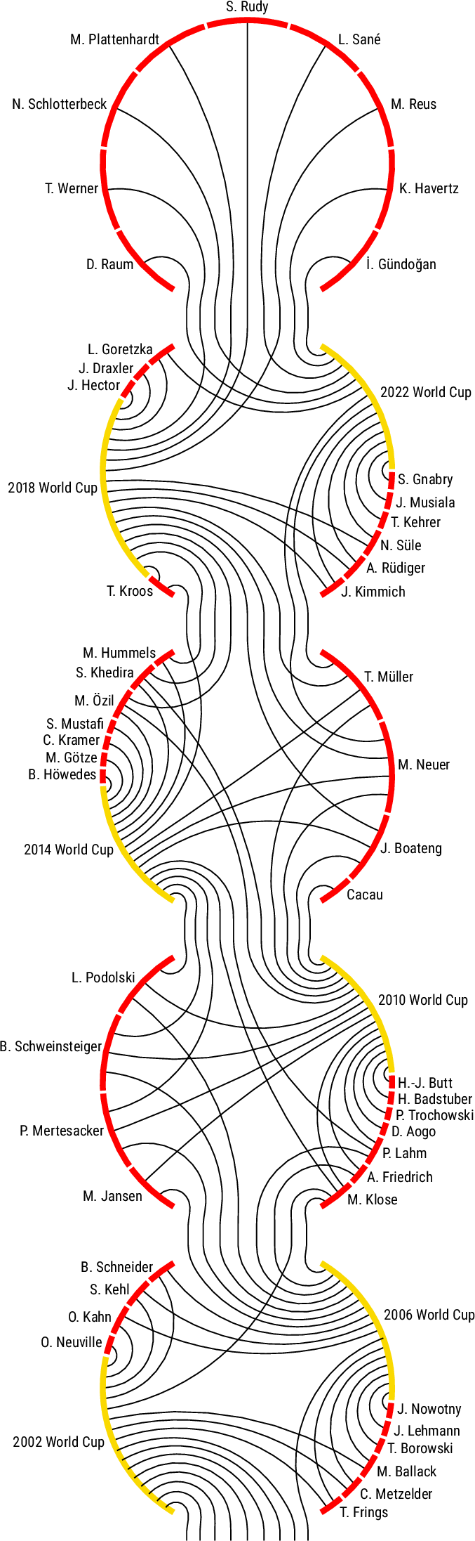
Figure 4: No caption.
Figure 5: Chunky Chains of player appearances at FIFA World Cups between 1990 and 2022. (a) 88 players and 9 World Cups with \(c = 12\); (b) 64 players and 7 World Cups with \(c = 8\).. a — Germany men’s national football team, b — United States women’s national soccer team
5 Case Study: Player Appearances at FIFA World Cups↩︎
Some graphs have a natural ordering of their nodes. We believe that Chunky Chains can help to reveal it [tkey:T2]. For our case study, we created bipartite graphs of football players and FIFA World Cups where an edge denotes the appearance of a player in the starting squad of any game at the respective World Cup. While Wold Cups have a strict temporal ordering, players appear at different competitions depending on the course of their career. We expect that our algorithms are able to order the World Cups by year only based on the player appearances. We use the dataset from [41]. 5 shows the graphs for two of the teams as Chunky Chains (see [42] for more).
In both drawings, the World Cups are ordered chronologically. With a capacity of twelve players per bucket, the drawing in 5 (a) requires no long edge. The drawing in 5 (b) contains three long edges and uses a capacity of eight players per bucket. In both cases, almost all edges are short [tkey:M2]. Since the crossings are contained in the chord diagrams, and Chunky Chains enforce a vertical structure, edges are easy to follow. Chunky Chains benefit from the way long edges are handled. By drawing them only partially and excluding them from the main layout process, the remaining graph can be arranged more freely.
We compare our drawings with three standard graph drawing approaches, (i) a two-track hierarchical layout produced by Graphviz’ dot engine, (ii) a force-directed layout produced by Graphviz’ neato engine, and (iii) a matrix
representation (see 10 and the supplementary material [42]).
The two-track layout (see 13) captures the temporal order of the World Cups well. Having two strictly separate tracks, highlights the bipartition of the input. However, it introduces a large amount of whitespace and many edge crossings (even some double crossings), which makes it difficult to follow individual player appearances. The edges are also quite long. In comparison, Chunky Chains utilize space more efficiently.
The force-directed layout (see 14) produces a compact drawing. While there is, to a certain extent, a temporal structure in the drawing, it is not easily recognizable. Moreover, edges are often routed in a complicated way. Partial overlaps of the edges make connections ambiguous and seriously hinder comprehensibility.
The matrix representation (see 1 2) displays the chronological order of the World Cups and shows the bipartite structure clearly. Because of the sparsity of our graphs, the space is not used efficiently. Since the drawing is relatively long, it is difficult to follow a column and correctly identify the row of a certain entry.
This case study suggests that Chunky Chains are capable of revealing linear structures [tkey:T2] while avoiding some drawbacks of the standard approaches.
6 Experiments↩︎
We conducted experiments to answer two research questions. The first one is, (RQ1) do commonly drawn graphs allow for good Chunky Chain drawings? We have established that graphs with a low
bucketwidth (or few long edges with respect to a given bucket capacity) benefit our drawing style [tkey:M1]. Thus, our second question is: (RQ2) are the methods presented in 4.1 capable of finding good bucket arrangements?
Benchmark Sets.
We used two datasets. Firstly, we evaluated our algorithms on the well-known Rome Graphs [43], a collection of 11,531 mostly real networks. Secondly, we generated a synthetic dataset of 1,170 \(k\)-paths (edge-maximal graphs of pathwidth \(k\)) with 10 to 200 vertices and \(k\in\{3,5,7\}\). From [obs:bi] (i) we know that bounded pathwidth is not necessarily helpful when solving Bucket Integrity and 3 only shows that pathwidth is bounded by bucket capacity and number of long edges (not vice versa). Nonetheless, the pathwidth is an established measure for how path-like a graph is, and therefore it is intuitive that graphs with bounded pathwidth may have good Chunky Chain visualizations. 6 shows the edge density distribution for the two datasets.
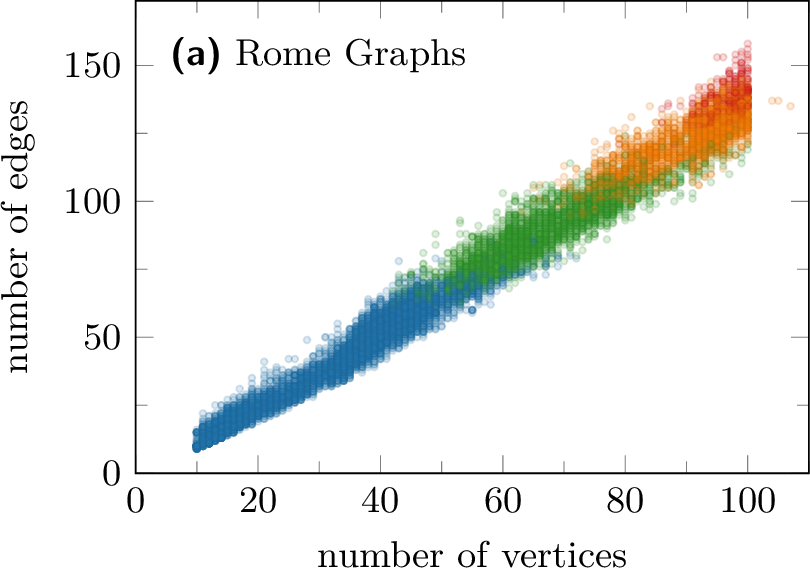
Figure 6: Number of vertices and edges for each graph in the two datasets. Graphs that could be solved to optimality for \(c\in\{4,8,12\}\) within one hour have blue markers, for \(c\in\{8,12\}\), they have green markers, and for \(c=12\), they have orange markers. Otherwise, they have red markers..
Benchmarking Environment.
We implemented the algorithms from 4.1. We used Gurobi optimizer 13.0.11 and HiGHS 1.14.02 [44] for ILP-solving and set a time limit of one hour for both. We call them Gurobi
and HiGHS, respectively. For our experiments, we used a set of identical compute nodes each running Debian 13 with Linux 6.12 on two AMD EPYC™ 9654 96-core processors alongside 1 TiB of RAM. Each solver job had exclusive access to eight cores
and 16 GiB of RAM (four cores and 8 GiB of RAM) for Gurobi (HiGHS). While Gurobi made use of all eight cores, we could not manage to get HiGHS use more than two cores. Both solvers used less than 4 GiB of RAM with all our instances.
We solve Ordered Bucket Integrity to obtain a heuristic solution for Bucket Integrity and use the following strategies to determine the vertex order. Two are heuristics for bandwidth
minimization, Cuthill-McKee[45] (cmk) and node centroid hill climbing [46], [47] (nchc). The third one is principal component analysis [48] (pca) – a method for dimensionality reduction – applied on the all-pairs shortest path matrix of \(G\). We
order the vertices by the first principal component.
The heuristics perform poorly on instances with many long edges. We therefore combine them with the meta-heuristic described in 4.1 and call the combined approaches cmk*, nchc*, and
pca*, respectively.
We implemented the ordering heuristics and the meta-heuristic in the Scala programming language3. The experiments concerned with the heuristics were conducted on a machine running Fedora 43 with Linux 7.0 on a single AMD Ryzen™ 7 7840HS and 64 GiB of RAM. While these processors share the ZEN4 micro-architecture, a difference in performance is expected. However, the results shown in 10 span seven orders of magnitude, so we consider it negligible.
Results.
We tried to find optimal bucket arrangements for the graphs in our datasets and \(c\in\{4,8,12\}\). We removed trivial instances where \(n\leq 2c\). Somewhat expected, our experiments show that it is easier to find such arrangements for larger capacities. The colors in 6 show which instances we could solve to optimality within one hour. Two patterns become apparent. Firstly, the stripes of equal color (i.e., instances that could be solved for the same capacities) are almost horizontal. This suggests that the number of edges, rather than the number of vertices, characterizes more difficult instances. Secondly, the inherent structure of the \(\{3,5,7\}\)-paths seems to help to solve Bucket Integrity for significantly larger instances (in terms of number of edges). [fig:cml-rome,fig:cml-kpaths] show that instances that require many long edges are also harder to solve.

Answering [tkey:RQ1], we can see in [fig:cml-rome] that the majority of the Rome Graphs can be drawn without long edges using capacity 8 and with less than ten long edges using capacity 4. 8 shows the normalized number of long edges for the \(\{3,5,7\}\)-paths. The box plots show little dispersion which advocates a linear correlation between the number of long edges and the number of edges, for constant capacity \(c\) and constant pathwidth. We also see that at least empirically, there is a connection between these parameters.
Regarding [tkey:RQ2], we assess the quality of our methods by measuring the normalized number of unnecessarily long edges, \((\ell_{\mathrm{heur}}-\ell_{\mathrm{opt}})/m\), where \(\ell_{\mathrm{heur}}\) is the number of long edges produced by the respective (heuristic) method and \(\ell_{\mathrm{opt}}\) is the optimum. We compared instances where we could not prove optimality to the best result of all methods. [fig:heur-rome,fig:heur-kpaths] show the results.
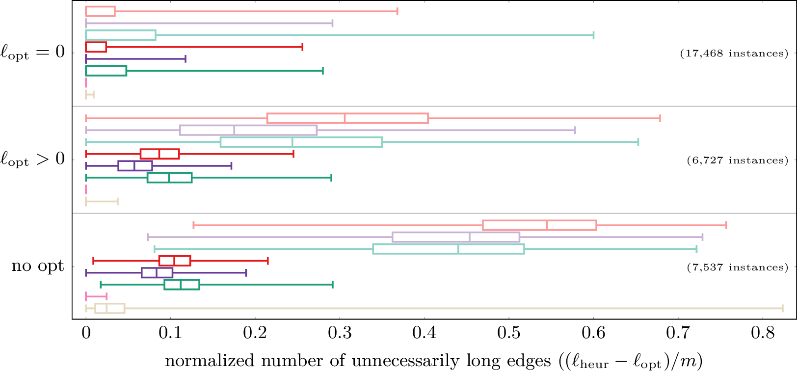
Figure 9: Quality of the heuristics on the two datasets measured as percentage of unnecessarily long edges \(\left((\ell_{\mathrm{heur}}-\ell_{\mathrm{opt}})/m\right)\). The bottommost set of box plots (no opt) contains instances that we could not solve to optimality. We compare them to the best known result.. a — Rome Graphs, b — \(\{3,5,7\}\)-paths
If \(\ell_{\mathrm{opt}}=0\), our heuristics find the optimal solution more often than not. Using the meta-heuristic is universally beneficial. The difference is particularly pronounced when \(\ell\) is large. At least on the Rome Graphs, HiGHS reliably finds (near-)optimal results. It is, however, very slow (see 10). Of the heuristics, nchc* outperforms the
others. While not quite as good, cmk* is much faster.

Figure 10: Running times per share of the dataset. The y-axis is logarithmic..
7 Conclusion and Future Work↩︎
We introduced a new visualization paradigm called Chunky Chains which is suitable for displaying graphs on narrow screens. We presented exact algorithms and a pipeline for drawing Chunky Chains in practice. Our experiments show that many real-world graphs can be drawn as Chunky Chains with small capacity. However, we leave several questions open.
Solvers have trouble finding good bounds with our ILP formulation. The large number of variables with non-integral values suggests that the model is weak. Can we strengthen it?
Is there a faster exact algorithm for minimizing crossings given a bucket arrangement?
The meta-heuristic for Bucket Integrity removes edges until it finds a bucket arrangement with zero long edges. Sometimes, terminating earlier gives a better solution. Can we identify such cases beforehand?
Can all outerplanar graphs be drawn as planar Chunky Chains?
We can make Chunky Chains even narrower when we use confluent edges (see 9). How does this impact the comprehensibility of our drawing style? Is it worth the increased cognitive load?
8 Spatial Color Co-occurrence Graphs↩︎
Spatial color co-occurrence graphs are inspired by Art Palette4, a tool for searching art collections for artworks that match a certain color combination. Our use case, however, is different. We are interested in colors that often occur in close proximity to each other. We visualize them with Chunky Chains (see the examples shown in 1 11)5.

We process the artworks as follows. We first downscale the image in order to speed up later steps and to smooth out artifacts like craquelure. Then, we apply a quantization filter6 based on the octtree algorithm [49] to reduce the image to a small set of colors. We now build a co-occurrence matrix of colors by going through all pairs of adjacent pixels and count how often color \(a\) is next to color \(b\). We remove all but the largest entries such that the remaining entries account for 95 % of the pixel transitions. Finally, we interpret the matrix as adjacency matrix and keep the largest connected component.
This type of graph can be used by artists as inspiration to find harmonic color combinations based on previous work. Also, such drawings can facilitate master studies of artists (and artworks) as contrasts, color schemes, the color key (major or minor), and value grouping may be easily revealed with our drawings.
9 Confluent Chunky Chains↩︎
With conventional Chunky Chains, the drawing’s width is \(O(c^2)\), for a given capacity \(c\). We can reduce the width to \(O(c)\) by allowing confluent edges. We assign edges to “tracks” such that, intuitively, two vertices are connected if a train can travel along that track, i.e., it does not make sharp turns. See 12 for a confluent version of 1.
Observe that for any two adjacent buckets \(B_i\) and \(B_{i+1}\), if we restrict \(G\) to only the edges connecting vertices in \(B_i\) with vertices in \(B_{i+1}\), the resulting subgraph \(G'\) is bipartite. We use a technique presented by Eppstein, Goodrich, and Meng [50], [51] to draw \(G'\) confluently. The number of tracks necessary equals the size of a biclique cover of \(G'\). Note that the size of the smaller bipartition bounds the size of the biclique cover. Finding a biclique cover of minimum size, however, is -hard, even for bipartite graphs [52].
While drawing edges confluently can obviously help with reducing the number of gate transitions [tkey:M2], it can also reduce the number of crossings [tkey:M3].
10 Supplemental Figures Concerning 5↩︎
See 13 14 1 2 on the following pages.

Figure 14: Two drawings of the graphs from 5 using the neato engine for force-directed layouts.. a — Germany men’s national football team (same graph as 5
(a))., b — United States women’s national soccer team (same graph as 5 (b)).
| N. Süle | |||||||||
| K. Havertz | |||||||||
| L. Sané | |||||||||
| D. Raum | |||||||||
| L. Goretzka | |||||||||
| A. Rüdiger | |||||||||
| S. Rudy | |||||||||
| J. Kimmich | |||||||||
| İ. Gündoğan | |||||||||
| J. Draxler | |||||||||
| S. Gnabry | |||||||||
| N. Schlotterbeck | |||||||||
| J. Musiala | |||||||||
| T. Kehrer | |||||||||
| M. Plattenhardt | |||||||||
| T. Werner | |||||||||
| J. Hector | |||||||||
| M. Reus | |||||||||
| T. Kroos | |||||||||
| M. Neuer | |||||||||
| M. Hummels | |||||||||
| M. Özil | |||||||||
| T. Müller | |||||||||
| J. Boateng | |||||||||
| S. Khedira | |||||||||
| Cacau | |||||||||
| M. Götze | |||||||||
| C. Kramer | |||||||||
| S. Mustafi | |||||||||
| B. Höwedes | |||||||||
| P. Lahm | |||||||||
| M. Jansen | |||||||||
| P. Mertesacker | |||||||||
| P. Trochowski | |||||||||
| H.-J. Butt | |||||||||
| M. Klose | |||||||||
| A. Friedrich | |||||||||
| B. Schweinsteiger | |||||||||
| L. Podolski | |||||||||
| D. Aogo | |||||||||
| H. Badstuber | |||||||||
| C. Metzelder | |||||||||
| O. Neuville | |||||||||
| O. Kahn | |||||||||
| S. Kehl |
continued on the following page
| T. Davidson | |||||||
| C. Dunn | |||||||
| L. Horan | |||||||
| A. Dahlkemper | |||||||
| C. Press | |||||||
| K. O’Hara | |||||||
| M. Pugh | |||||||
| J. Ertz | |||||||
| T. Heath | |||||||
| M. Brian | |||||||
| S. Mewis | |||||||
| R. Lavelle | |||||||
| B. Sauerbrunn | |||||||
| M. Klingenberg | |||||||
| A. Krieger | |||||||
| M. Rapinoe | |||||||
| L. Holiday | |||||||
| A. Naeher | |||||||
| A. Rodriguez | |||||||
| A. Morgan | |||||||
| S. Leroux | |||||||
| C. Lloyd | |||||||
| H. Solo | |||||||
| N. Kai | |||||||
| H. O’Reilly | |||||||
| A. Wambach | |||||||
| R. Buehler | |||||||
| A. LePeilbet | |||||||
| C. Rampone | |||||||
| S. Boxx | |||||||
| L. Lindsey | |||||||
| K. Markgraf | |||||||
| L. Chalupny | |||||||
| C. Parlow | |||||||
| C. Whitehill | |||||||
| M. Dalmy | |||||||
| A. Wagner | |||||||
| S. Cox | |||||||
| L. Osborne | |||||||
| B. Scurry | |||||||
| T. Roberts | |||||||
| K. Lilly | |||||||
| M. Hamm | |||||||
| T. Milbrett | |||||||
| B. Chastain | |||||||
| K. Bivens | |||||||
| J. Foudy | |||||||
| J. Fawcett | |||||||
| S. Higgins | |||||||
| S. Webber | |||||||
| T. Venturini | |||||||
| H. Manthei | |||||||
| T. Staples | |||||||
| L. Hamilton | |||||||
| D. Belkin | |||||||
| A. Cromwell | |||||||
| C. Overbeck | |||||||
| C. Jennings-Gabarra | |||||||
| W. Gebauer | |||||||
| T. Bates | |||||||
| M. Akers | |||||||
| L. Henry | |||||||
| M. Harvey | |||||||
| A. Heinrichs |
References↩︎

Find digital versions of “Starry Night Over the Rhône” at https://artsandculture.google.com/asset/uQE3XORhSK37Dw and of “Still Life with Asphodels” at https://artsandculture.google.com/asset/rwHGE7FnTOc2wQ.↩︎
We use the implementation provided with https://sksamuel.github.io/scrimage/.↩︎