Drift Happens: An Empirical Study of Neural Architecture Robustness to Temporal Distribution Shift
July 07, 2026
Abstract
Real-world data distributions evolve over time, inducing temporal distribution shift that can substantially degrade the reliability of deployed machine learning systems. However, the extent to which architectural choices and their associated inductive biases affect temporal robustness remains insufficiently understood.
We present a systematic empirical comparison of temporal robustness across three heterogeneous, time-indexed domains encompassing image classification, multi-label text classification, and text regression tasks. Using a unified evaluation framework based on temporal drift matrices, we train models on cumulative historical data and evaluate their performance on both earlier and later time periods, thereby quantifying cross-temporal generalization. Our study spans model families ranging from simple multilayer perceptrons and convolutional networks to recurrent networks and pretrained Transformer-based encoders.
Collectively, the results show that architectural inductive biases systematically shape temporal robustness: models whose inductive biases lead them to exploit localized, highly discriminative features attain the highest in-distribution accuracy, yet those features are often the ones that change most over time, so these models degrade fastest, while pretrained encoders that draw on coarser, more stable representations drift more gradually. These observations offer practical guidance for selecting architectures for real-world systems subject to temporal drift.
1 Introduction↩︎
Machine learning models are typically trained under the assumption that training and test data are drawn from the same distribution. In practice, this assumption rarely holds: real-world data evolves over time, exhibiting temporal distribution shift that can degrade model performance in ways that standard held-out evaluation fails to capture. A model that achieves high accuracy on held-out data from the same time period may fail when deployed on future inputs.
While distribution shift is well-documented, less understood is how architectural choices influence a model’s robustness to temporal drift.
Do different inductive biases (the translation invariance of convolutions, the sequential modeling of recurrent nets, the attention of Transformers) lead to different rates of temporal degradation?
Do frozen, pretrained encoders resist temporal drift better than models trained end to end?
These questions have practical implications for model selection, yet systematic comparisons across architectures and domains remain scarce.
This work investigates the temporal robustness of neural classifiers across three domains: image classification (Yearbook), text regression (Amazon Reviews), and multi-label text classification (arXiv). For each
domain, we evaluate diverse architectures, from simple baselines to pretrained transformers, using a unified framework based on temporal drift matrices and provide qualitative explanations for model degradation via gradient saliency maps. Our contributions
are threefold:
We provide a unified empirical assessment of temporal robustness across three long-range, time-indexed domains, enabling direct comparison of how neural architectures behave under temporal distribution shift.
We organize time-indexed evaluation in the spirit of Wild-Time [1] into temporal drift matrices, a compact representation that quantifies cross-temporal generalization by measuring performance when training on cumulative historical data and testing on both earlier and later time periods.
We systematically compare a broad spectrum of model families, from multilayer perceptrons, convolutional and residual networks, and recurrent networks to transformers trained on the data and frozen pretrained encoders, highlighting how architectural assumptions relate to degradation patterns across modalities and tasks.
Taken together, our results characterize how performance deteriorates as the temporal gap between training and evaluation widens across domains and model classes. The features an inductive bias extracts within the training period are what lift in-distribution performance, yet they are the most tied to it and the first to degrade as the data drifts, so the very features that make a model accurate in distribution are the least robust over time. Frozen pretrained encoders, relying on coarser and more transferable representations, trade in-distribution accuracy for steadier degradation. These findings guide architecture selection in non-stationary real-world environments.
2 Background and Related Work↩︎
2.1 Temporal Distribution Shift↩︎
A central challenge in real-world machine learning systems is that the data-generating process is rarely stationary. As models are deployed over months, years, or decades, both inputs and label semantics may evolve, causing systematic discrepancies between distributions encountered during training and those observed at inference. Such temporal evolution, commonly referred to as temporal distribution shift, is pervasive across domains. Understanding the structure of this shift is essential for assessing and improving temporal robustness. However, prior work has largely focused on static or domain-level distribution shifts [2]–[4], with limited attention to drift that unfolds sequentially over time, particularly in non-generated, in-the-wild settings [1].
Following established terminology in concept drift research [5], temporal distribution shift can be characterized along three complementary axes (Figure 1):
Covariate shift occurs when the input distribution \(P(X)\) changes while the conditional \(P(Y \mid X)\) remains fixed. This type of shift commonly arises in natural data streams where observational setups, sociocultural conventions, or user behavior gradually evolve.
Label shift refers to changes in the marginal label distribution \(P(Y)\). Long-term textual or behavioral datasets frequently exhibit such imbalance drift as the prevalence of topics, categories, or rating patterns changes over time.
Concept drift denotes changes in the conditional distribution \(P(Y \mid X)\), implying that identical inputs may correspond to different labels at different time points. This form of drift is particularly pronounced in domains where semantics or visual attributes evolve, such as historical portraits [6] or online platforms.
In practice, these forms of drift rarely occur in isolation and often manifest in combination [7]. As a result, the temporal robustness of a model depends not only on the magnitude of drift but also on how its architectural assumptions and inductive biases interact with the evolving data distribution.
2.2 Model Robustness to Distribution Shift↩︎
![Figure 1: Drift types in a binary classification setting. Circles and stars indicate the label classes; the curve represents the decision boundary. Concept drift induces a change in the decision boundary, Covariate drift (virtual drift) changes the input distribution, and Label drift alters the relative class frequency [8].](/article/2607.05908/_pdflatex/xgtsynfv.png "fig:")
Understanding how learning algorithms behave under distribution shift has become an important research direction. Early work approached robustness through domain adaptation [2] and out-of-distribution generalization [3], formalizing shift as a
transition between a small number of discrete source and target domains. The introduction of large-scale benchmarks such as WILDS [4],
which focuses on naturally occurring distribution shifts without explicit temporal indexing, and more recently Wild-Time [1],
which explicitly models time-indexed data and temporal distribution shifts, has broadened this perspective by providing evaluation protocols that more closely reflect real-world deployment scenarios.
A complementary line of research has examined robustness through model diagnostics and monitoring. Methods for detecting drift onset by examining changes in latent representations or predictive uncertainty have shown promise in deep learning settings [9], [10]. Recent empirical analyses have characterized how concept drift manifests in practice, including its locality and temporal progression across large-scale data streams [7]. At the systems level, work on data-centric and continual-learning infrastructures has explored how to maintain model quality over time through cost-aware retraining and pipeline orchestration [8], [11]–[14].
Despite these advances, robustness studies commonly focus either on a single architecture evaluated across multiple datasets or on a single dataset used to compare a narrow set of architectures. As a result, comparatively little is known about how architectural design choices interact with long-range temporal drift across heterogeneous modalities and tasks. This gap is particularly relevant given the diversity of inductive biases exhibited by modern neural models: convolutional networks encode locality and translation equivariance, recurrent networks capture sequential structure [15], [16], and Transformer-based encoders rely on self-attention with minimal structural priors [17]. Likewise, large-scale pretraining in vision and language [18], [19] introduces representations shaped by broad historical data, yet their behavior under extended temporal drift remains poorly characterized.
The present study addresses this open question by comparing these architectural families under a shared temporal evaluation protocol and across multiple modalities, enabling a controlled analysis of how model design influences robustness under real-world temporal distribution shift.
2.3 Robustness Evaluation vs.Temporal Adaptation↩︎
This work evaluates the inherent temporal robustness of neural architectures under distribution shift, measuring how different model families, trained only on cumulative historical data, perform as the temporal gap between training and evaluation widens. This isolates the robustness arising from architectural design and pretraining alone, prior to any adaptive intervention.
A complementary line of research instead investigates how models can adapt once drift is detected, through scheduled or cost-aware retraining [11], [12], continual-learning pipelines [8], [13], [14], or accuracy-aware data maintenance [20], addressing when to retrain, how much data to incorporate, and how to trade performance against cost. Our study is orthogonal to that literature and provides a foundation on which such adaptation strategies can be designed, evaluated, and compared.
3 Methods and Experimental Approach↩︎
Temporal distribution shift manifests differently across modalities, tasks, and time scales, yet existing empirical studies typically vary a single axis at a time, leaving open how architectural design, label structure, and drift mechanism jointly shape temporal robustness (Section 2). Our setup targets exactly this cross-cutting comparison: we combine three long-range, time-indexed datasets with a diverse suite of neural architectures spanning multiple inductive biases, all evaluated under the unified temporal protocol of Section 4 (temporal drift matrices), so that architectural differences, rather than differences in splitting or evaluation, drive the observed robustness patterns.
3.1 Datasets↩︎
Our empirical analysis spans three qualitatively distinct temporal scenarios, chosen to cover different modalities, tasks, and sources of distribution shift. Each dataset captures multiple decades of real-world temporal evolution, making it suitable for cross-temporal evaluation.
3.1.1 Yearbook: A Century of Portraits↩︎
The Yearbook dataset [21] contains 37,921 frontal portraits of American high-school seniors from
valstore/yearbook/cutoff-firstvalstore/yearbook/cutoff-first to valstore/yearbook/cutoff-lastvalstore/yearbook/cutoff-last , which we align and process as 3-channel \(32\times32\) tensors. Although acquisition is largely
standardized, stylistic attributes (e.g., hairstyles, clothing, accessories) vary substantially across decades. The dataset provides binary sex labels that are approximately balanced over time. It is a canonical benchmark for temporal shift: Wild-Time
[1] uses a pre-/post-1970 split and reports marked out-of-distribution degradation, and Modyn [14] observes accuracy decay as the train–test time gap grows. We reproduce this trend (Fig. 2), consistent with
covariate and concept drift.
3.1.2 Amazon Reviews 2023: E-commerce↩︎
The Amazon Reviews dataset [22] comprises 571.54 million reviews across 33 product categories, spanning May 1996 to September
2023. Each review has a timestamp, star rating, and free-text content. We cast a review-level sentiment regression task, predicting the 1–5 rating from the text, which exhibits strong covariate and concept drift due to evolving language, consumer behavior,
and platform usage. We focus on seven categories, restrict to 2014–2023, and draw a stratified sample of 300,000 reviews.
3.1.3 arXiv: Scientific Discourse↩︎
The arXiv dataset [23] defines a multi-label task over 2,866,787 title–abstract records annotated with 176 subject categories. We
concatenate titles and abstracts, keep seven leaf categories (11), and use valstore/arxiv/cutoff-firstvalstore/arxiv/cutoff-first – valstore/arxiv/cutoff-lastvalstore/arxiv/cutoff-last submissions whose categories fall
within them (papers may carry several). Category mix and terminology shift, inducing label and covariate drift[8]. Wild-Time
[1] reports roughly 20% degradation under temporal splits for a related arXiv task, and the gap is not substantially closed by domain
generalization or continual learning methods, motivating our architectural comparison.
3.2 Model Implementation↩︎
We evaluate architectures spanning different inductive biases to understand how model design affects temporal robustness. Rather than covering the full architecture landscape, we select families that span the spectrum of inductive-bias strength: from simple baselines without structural assumptions that establish lower bounds on performance, to modern architectures that incorporate structural priors, to pre-trained models that leverage large-scale external data. This spread is what lets us attribute robustness differences to the priors themselves.
3.2.1 Image Classification↩︎
For the Yearbook dataset, we evaluate four model families trained on the data, each at three sizes (small, medium, large), for valstore/yearbook/scratch-modelsvalstore/yearbook/scratch-models architectures, complemented by
valstore/yearbook/frozen-modelsvalstore/yearbook/frozen-models pretrained vision encoders used as frozen backbones.
The four families differ in the spatial prior they encode. At one extreme, the multilayer perceptron (MLP) flattens the image and applies only fully connected layers, imposing no spatial structure. The convolutional
network (CNN) builds in locality and translation equivariance through convolutional filters with batch normalization and pooling, and the residual network (ResNet) extends it with skip connections [24] that ease optimization at greater depth. At the other extreme, the vision Transformer (ViT) drops convolution for
self-attention over patches [25], a far weaker spatial prior, with a small patch size suited to the \(32\times32\) inputs. Across all four, the small, medium, and large variants scale depth and width.
Finally, we assess transfer learning using pretrained vision encoders trained on large-scale curated or web-scale datasets. The underlying hypothesis is that representations learned from diverse data may exhibit stronger temporal robustness
than features learned solely from historical portraits. We consider valstore/yearbook/frozen-modelsvalstore/yearbook/frozen-models pretrained models. The self-supervised DINOv2-S [26] and DINOv3-S [27] are pretrained on large curated image
collections; CLIP-B32 [28] and SigLIP-B [29] use contrastive image-text pretraining, the latter with a sigmoid loss; ConvNeXt-S [30], ResNet50-IN [24], and ViT-S16-IN21k [25] are trained with supervised ImageNet labels, the last on ImageNet-21k; and MAE-B [31] and EVA02-B [32] are pretrained with masked
image modeling. In all cases, we freeze the pretrained backbone and train only a linear classification head, isolating the contribution of pretrained representations from the effects of fine-tuning dynamics.
3.2.2 Text Models↩︎
For the Amazon Reviews and arXiv datasets, we evaluate model families that differ in their inductive biases for representing textual structure. The same architectures serve both datasets, differing only in output layer and
loss, with Amazon Reviews using regression under a weighted mean squared error and arXiv multi-label classification under a weighted binary cross-entropy.
All four families operate on cached RoBERTa token embeddings. The feed-forward baseline (FFN) averages them into a single 768-dimensional vector and passes it through a small MLP head that discards order entirely, with
variants scaling the hidden width from 128 to 2048. The convolutional model (TextCNN) [33] applies
one-dimensional convolutions to capture local n-gram patterns, scaling the number and width of its filters. The recurrent models read the sequence token by token, as a single-layer bidirectional GRU [16], a single-layer bidirectional LSTM [15], and a two-layer bidirectional LSTM with attention. The Transformer encoders replace recurrence with self-attention [17] and learnable positional embeddings, ranging from 1 to 5 layers and 4 to 6 heads.
Finally, we assess transfer learning from pretrained language encoders. We consider frozen encoders with a light head trained on the pooled output: BERT [18], RoBERTa [19], DeBERTa-v3 [34], ELECTRA [35], MPNet [36], ModernBERT [37], and
DistilBERT [38] on both text tasks, plus MiniLM-L6 [39] on arXiv. As with the vision encoders, freezing isolates pretrained representations from fine-tuning.
4 Evaluation Framework↩︎
Standard held-out evaluation measures performance on data from the training distribution, which under temporal shift can look strong even as the model fails on future data. We therefore measure cross-temporal generalization explicitly.
4.1 Temporal Drift Matrices↩︎
Let \(\mathcal{D} = \{(x_i, y_i, t_i)\}_{i=1}^{N}\) denote a dataset where each example is associated with a timestamp \(t_i\). We divide the timeline into \(K\) disjoint intervals \(\mathcal{T} = \{T_1, \ldots, T_K\}\), where \(T_k = [t_k^{\text{start}}, t_k^{\text{end}})\). Let \(\mathcal{D}_k = \{(x, y, t) \in \mathcal{D} : t \in T_k\}\) denote the subset of data from interval \(k\).
For training, we construct cumulative datasets \(\mathcal{D}_{\leq k} = \bigcup_{j=1}^{k} \mathcal{D}_j\) containing all data up to and including interval \(k\). A model \(f_k\) trained on \(\mathcal{D}_{\leq k}\) has access to historical data over time \(t_k^{\text{end}}\) but no knowledge of future periods. This cumulative strategy reflects realistic deployment scenarios in which models are periodically retrained on all historical data.
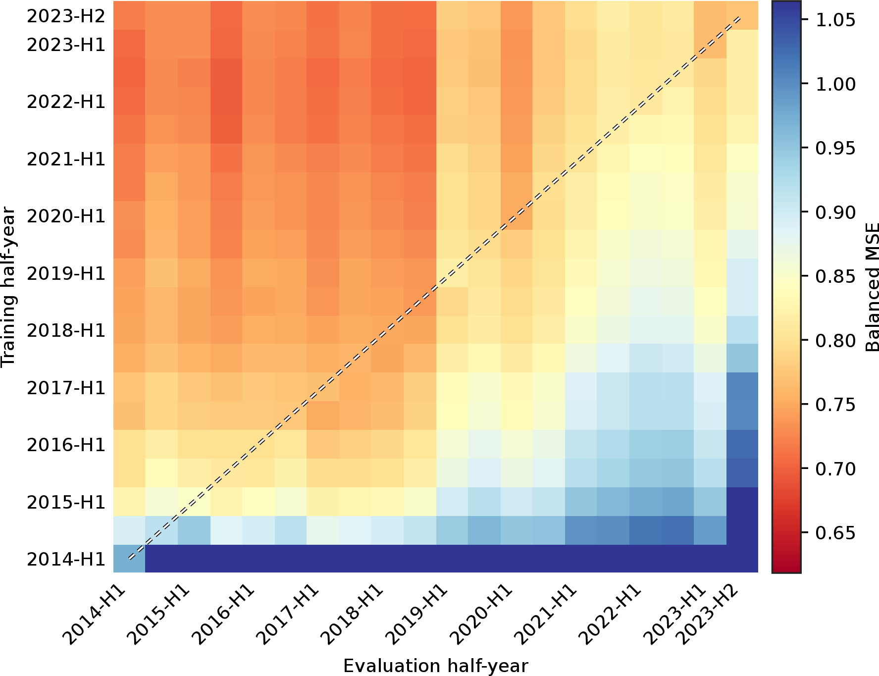
The temporal drift matrix \(M \in \mathbb{R}^{K \times K}\) captures cross-temporal generalization: \[M_{ij} = \text{perf}(f_i, \mathcal{D}_j)\] where \(\text{perf}(\cdot, \cdot)\) denotes a performance metric (accuracy, macro AUC, or balanced MSE depending on the task). Entry \(M_{ij}\) measures how well a model trained on data through period \(i\) performs on data from period \(j\).
The structure of \(M\) reveals aspects of temporal robustness. Following our plotting convention, rows are the training cutoff (“trained up to”) and columns the evaluation period (“evaluated on”), with time increasing upward and to the right from a lower-left origin. The diagonal \(M_{ii}\) is in-distribution performance on data held out from the training period; the upper-left (\(j < i\)) is held-out performance on earlier in-training periods; and the lower-right (\(j > i\)) is forward generalization to data unseen during training. This lets us read how performance degrades (or improves) as the temporal gap between training and evaluation widens.
4.2 Temporal Splitting Strategy↩︎
Each slice \(\mathcal{D}_k\) is partitioned once into a stratified training split \(\mathcal{D}_k^{\text{train}}\) (70%) and a held-out test split \(\mathcal{D}_k^{\text{test}}\) (30%), shared across all models via a fixed split seed. For in-distribution evaluation (when \(j \leq i\)), we use only the held-out test split of \(\mathcal{D}_j\) to prevent data leakage:
\[\nonumber \mathcal{D}_{\text{eval}}^{(i,j)} = \begin{cases} \mathcal{D}_{j}^{\text{test}} & \text{if } j \leq i \text{ (in-distribution)} \\ \mathcal{D}_{j}^{\text{train}} \cup \mathcal{D}_{j}^{\text{test}} & \text{if } j > i \text{ (out-of-distrib.)} \end{cases}\]
For out-of-distribution evaluation on future time slices, we use all available samples from that period to maximize statistical power, since by definition none of this data was seen during training. Evaluating on periods that overlap the training data (\(j \leq i\)) is deliberate: these held-out entries verify that a model retains performance across the historical periods it was trained on and provide the in-distribution reference from which forward decay is measured.
4.3 Training Protocol↩︎
The image models are trained with Adam [40] and the text models with its decoupled-weight-decay variant AdamW, a standard choice that
behaves robustly across heterogeneous architectures; fixing one optimizer per modality avoids per-model optimizer tuning as a confound. Learning rates are task-specific, with exact hyperparameters pinned in versioned experiment presets. Training proceeds
for a fixed number of epochs, and model selection is based on the final checkpoint. Every configuration is trained under multiple random seeds, five on Yearbook and three on the text tasks (7), and
all results average over seeds.
We adopt a cumulative temporal training strategy: for each slice \(T_k\) we train a model \(f_k\) on \(\mathcal{D}_{\leq k}\), all examples observed up to \(T_k\), yielding a sequence \(\{f_1, \dots, f_K\}\) that each represent the best model obtainable from the data available at that point in time. All checkpoints are stored and evaluated on every slice to construct the full temporal drift matrix \(M\).
The loss follows the task structure and is tailored to address label imbalance.
For binary classification on Yearbook, we minimize standard two-class cross-entropy on logits and labels, the maximum-likelihood objective for a two-class softmax model.
For multi-label classification on arXiv, each paper may belong to multiple subject categories. We keep only seven leaf categories as the label space, retaining papers that carry at least one of them. The label distribution remains
skewed, with negative examples substantially outnumbering positives for each category. We therefore use a weighted binary cross-entropy with logits, applied independently to each of the \(C = 7\) categories: \[\begin{align}
\mathcal{L}_{\text{BCE}} &= -\frac{1}{n}\sum_{i=1}^{n} \sum_{c=1}^{C} \big[ w_c \, y_{ic} \log(\sigma(z_{ic})) \\ &\qquad + (1-y_{ic}) \log(1-\sigma(z_{ic})) \big],
\end{align}\] where \(z_{ic}\) denotes the logit for class \(c\), \(\sigma(\cdot)\) is the sigmoid function, and \(y_{ic}
\in \{0,1\}\) is the binary label. The class weights \(w_c\) are defined as \[w_c = \frac{|\{i : y_{ic} = 0\}|}{|\{i : y_{ic} = 1\}|},\] i.e., the ratio of negative to positive
examples for each category. This reweighting compensates for label imbalance by amplifying the contribution of rare positive labels, preventing the model from achieving deceptively high accuracy by predicting the all-zero vector.
For regression on Amazon Reviews, we train models to predict the star rating using a weighted mean squared error: \[\mathcal{L}_{\text{WMSE}} = \frac{1}{n}\sum_{i=1}^{n} w_{y_i} (y_i -
\hat{y}_i)^2,\] where \(y_i \in \{1,2,3,4,5\}\) is the true rating and \(\hat{y}_i\) is the prediction. The rating-specific weights \(w_r\) are
defined as \[w_r = \frac{n}{n_r},\] with \(n\) the total number of samples and \(n_r\) the number of samples with rating \(r\). Because the empirical rating distribution is heavily skewed toward high scores, an unweighted MSE would be dominated by the majority class and largely ignore rare low-rating events. The inverse-frequency
weighting counteracts this imbalance, ensuring that errors on minority ratings remain visible in the objective and that temporal degradation in performance cannot be explained solely by changes in the prevalence of positive reviews.
4.4 Evaluation Metrics↩︎
To populate each entry of the drift matrix \(M\), we require a scalar performance metric per train-test time pair. We match each metric to the task’s label structure: accuracy for Yearbook, whose binary
labels are approximately balanced (8.1); balanced MSE (\(\text{MSE}_{\text{bal}}\)) for Amazon Reviews, which reweights its skewed rating distribution (8.2); and macro AUC (\(\overline{\text{AUC}}\)) for arXiv, whose imbalanced multi-label categories require a threshold-free, per-class average (8.3). The two classification tasks thus receive different metrics because their label structures differ; the drift protocol itself is identical.
4.5 Summary Statistics of the Drift Matrix↩︎
In the drift matrix \(M\), the row index \(i\) is the training cutoff and the column index \(j\) is the evaluation period, so the entry \(M_{ij}\) is the performance of a model trained on all data up to period \(i\) when it is tested on period \(j\).
Three numbers summarize the matrix, each averaged only over the cells that are filled, since a train-test pair with no completed run leaves its cell empty. The in-distribution score is the average of the diagonal, \[\mathrm{ID}(M) = \operatorname{mean}_{i} M_{ii}, \label{eq:in95distribution}\tag{1}\] a model’s performance on the same period it was trained through. The future score averages the cells with \(j > i\), where the evaluation period falls after the training cutoff, \[\mathrm{Fut}(M) = \operatorname{mean}_{j > i} M_{ij}. \label{eq:future}\tag{2}\] The decay is the difference between the two, oriented so a larger value always means worse temporal robustness, since accuracy and \(\overline{\text{AUC}}\) are better when high while \(\text{MSE}_{\text{bal}}\) is better when low, \[\mathrm{Dec}(M) = \begin{cases} \mathrm{ID}(M) - \mathrm{Fut}(M) & (\text{accuracy},\;\overline{\text{AUC}}),\\ \mathrm{Fut}(M) - \mathrm{ID}(M) & (\text{MSE}_{\text{bal}}). \end{cases} \label{eq:decay}\tag{3}\] so a positive decay is a loss of performance on future periods and a negative one, which is uncommon, a gain. Together, future score and decay order every model from most to least temporally robust.
Beyond these whole-matrix scores, we look at how robustness depends on the training time itself. Fixing one cutoff \(i\), a single row of the matrix, we pair its diagonal cell \(M_{ii}\) with the average over the later periods in that row (\(\operatorname{mean}_{j>i} M_{ij}\)) and the decay between them, reading these at a few cutoffs spread evenly across the timeline (the last one is left out, as it has no future). Averaging the same quantities within each architecture family lets us compare the families directly.
To place each model against the others, we average the matrices over the cohort \(\mathcal{C}\) of models into the cohort-mean matrix \[\bar{M}_{ij} = \frac{1}{|\mathcal{C}|}\sum_{m \in \mathcal{C}} M^{(m)}_{ij}, \label{eq:cohort95mean}\tag{4}\] defined at the cells every model fills; each model’s deviation is \(\Delta^{(m)}_{ij} = M^{(m)}_{ij} - \bar{M}_{ij}\).
5 Results↩︎
Each model is summarised through its drift matrix by the in-distribution, forward, and decay scores of 4.5, namely its performance on the period it was trained through, its mean performance on the later periods held out from training, and the difference between the two. How far a model degrades between them is governed by two factors that recur across the three domains, the strength of its inductive bias and whether it relies on a frozen pretrained encoder.

5.1 Image Classification↩︎
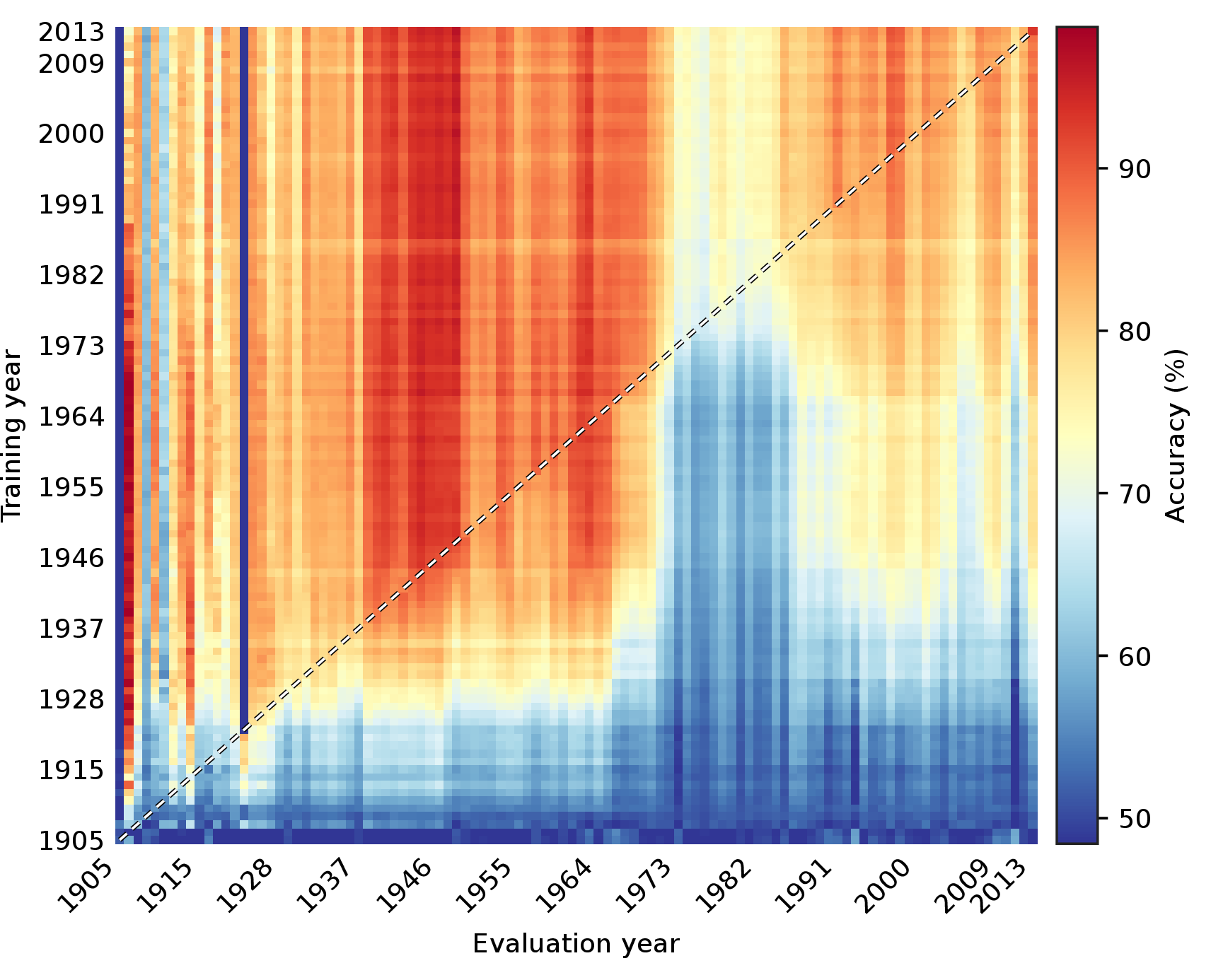
On Yearbook, the model families separate sharply in distribution, along the diagonal of the cohort-mean matrix in the Yearbook panel of 2. MLP-S, which flattens the image into a vector and
imposes no spatial structure, sits at about \(\ifcsname valstore/yearbook/model/mlp_s/indist\endcsname\csname valstore/yearbook/model/mlp_s/indist\endcsname \else\errmessage{unknown value key:
yearbook/model/mlp_s/indist}\fi\%\), while the CNNs and ResNets reach near \(\ifcsname valstore/yearbook/model/cnn_l/indist\endcsname\csname valstore/yearbook/model/cnn_l/indist\endcsname \else\errmessage{unknown value key:
yearbook/model/cnn_l/indist}\fi\%\) for CNN-M and CNN-L (¿tbl:tab:robustness95yearbook?). What sets these apart is their inductive bias toward locality and translation equivariance, by which they build features from small local
regions of the image and recognise a pattern wherever it appears, and this lets them exploit the cues that most sharply separate male from female portraits within a given period. The ViTs and frozen encoders fall between these two ends.
Temporal robustness reverses this ordering, and we read it from the decay, the accuracy a model loses once the evaluation year moves past its training cutoff (¿tbl:tab:robustness95yearbook?). The CNNs and ResNets, strongest in distribution, decay the most, by \(\ifcsname valstore/yearbook/model/cnn_l/decay\endcsname\csname valstore/yearbook/model/cnn_l/decay\endcsname \else\errmessage{unknown value key: yearbook/model/cnn_l/decay}\fi\) and \(\ifcsname valstore/yearbook/model/cnn_m/decay\endcsname\csname valstore/yearbook/model/cnn_m/decay\endcsname \else\errmessage{unknown value key: yearbook/model/cnn_m/decay}\fi\) points for CNN-L and CNN-M, so their accuracy on future years falls to about \(\ifcsname valstore/yearbook/model/cnn_l/future\endcsname\csname valstore/yearbook/model/cnn_l/future\endcsname \else\errmessage{unknown value key: yearbook/model/cnn_l/future}\fi\%\). MLP-S is the steadiest model of all, with only \(\ifcsname valstore/yearbook/model/mlp_s/decay\endcsname\csname valstore/yearbook/model/mlp_s/decay\endcsname \else\errmessage{unknown value key: yearbook/model/mlp_s/decay}\fi\) points of decay, though from its lower starting accuracy of \(\ifcsname valstore/yearbook/model/mlp_s/future\endcsname\csname valstore/yearbook/model/mlp_s/future\endcsname \else\errmessage{unknown value key: yearbook/model/mlp_s/future}\fi\%\). The frozen pretrained encoders form a third group, more stable than the CNNs but less accurate to begin with, decaying by \(\ifcsname valstore/yearbook/frozen/decay-min\endcsname\csname valstore/yearbook/frozen/decay-min\endcsname \else\errmessage{unknown value key: yearbook/frozen/decay-min}\fi\) to \(\ifcsname valstore/yearbook/frozen/decay-max\endcsname\csname valstore/yearbook/frozen/decay-max\endcsname \else\errmessage{unknown value key: yearbook/frozen/decay-max}\fi\) points, with the self-supervised DINOv3-S steadiest among them and the supervised ImageNet-21k backbone least.
What lifts a model in distribution is also what undermines it over time. The features a strong inductive bias extracts to separate the classes raise its in-distribution accuracy, but they are the most specific to the years it
was trained on, and the first to lose their meaning once hairstyles, clothing, and image quality drift. The sharper a model’s in-distribution lead, the faster it erodes as the data ages. Robustness on Yearbook is therefore not a
property an architecture optimises on its own, but the other side of fitting a single period too closely, closer to overfitting across time than across samples (9).
The forgetting curves in 4 show this playing out year by year. Each curve plots a model’s accuracy against the gap between its training cutoff and the evaluation year, so reading from left to right traces how quickly it forgets (9.7). The strongly biased networks start far above the rest, near \(90\%\) at a zero gap, and their curves descend the steepest. As the gap widens the curves draw together and then cross, so the families that led in distribution lose their edge on the most distant years, and every model settles near two-class chance.
5.1.1 Saliency Maps↩︎
The gradient saliency maps in 3 show where this fragility comes from. Extending the training window from 1950 to 1970 sharpens where the convolutional models look: the CNN tightens from a diffuse scatter over the cheeks and mouth to a compact, near-symmetric pair of bright spots at the eyes, the detail that most sharply tells the classes apart, and the ResNet shifts the same way while keeping a broader spread across the central face. The MLP, without that bias, spreads its attribution across the whole frame at either cutoff, the background included. The same precision that lets the convolutional models read this discriminative detail binds them to it: those localized features are the most specific to the training period and the most exposed to drift, while the MLP’s blunter reading is less tied to any era.
5.2 Text Models↩︎
Each text model is a light head trained on cached, frozen RoBERTa embeddings (3), a shared representation over which the families differ only in inductive bias. Amazon Reviews is a rating
regression scored by balanced MSE, where lower is better, and arXiv is a multi-label classification scored by macro AUC.
5.2.1 Amazon Reviews↩︎
On Amazon Reviews the recurrent and Transformer models fit the training reviews most closely, since both read the wording in context, the recurrent networks token by token and the Transformers through self-attention, and so capture how a
review’s words compose into its rating. That fit shows up as the lowest in-distribution error, down to \(\ifcsname valstore/amazon_reviews/model/bigru_s/indist\endcsname\csname
valstore/amazon_reviews/model/bigru_s/indist\endcsname \else\errmessage{unknown value key: amazon_reviews/model/bigru_s/indist}\fi\) balanced MSE for BiGRU-S, with the Transformers alongside them at \(\ifcsname
valstore/amazon_reviews/model/tx_s/indist\endcsname\csname valstore/amazon_reviews/model/tx_s/indist\endcsname \else\errmessage{unknown value key: amazon_reviews/model/tx_s/indist}\fi\) for TX-S (2,
¿tbl:tab:robustness95amazon95reviews?). The FFN, which averages the embeddings and discards word order, sits higher at about \(\ifcsname valstore/amazon_reviews/family/ffn/indist\endcsname\csname
valstore/amazon_reviews/family/ffn/indist\endcsname \else\errmessage{unknown value key: amazon_reviews/family/ffn/indist}\fi\), and the frozen encoders higher still, between \(\ifcsname
valstore/amazon_reviews/frozen/indist-min\endcsname\csname valstore/amazon_reviews/frozen/indist-min\endcsname \else\errmessage{unknown value key: amazon_reviews/frozen/indist-min}\fi\) and \(\ifcsname
valstore/amazon_reviews/frozen/indist-max\endcsname\csname valstore/amazon_reviews/frozen/indist-max\endcsname \else\errmessage{unknown value key: amazon_reviews/frozen/indist-max}\fi\).
Temporal robustness runs the other way, and the models that fit the reviews most tightly are the ones whose error grows fastest. The recurrent networks decay the most, by up to \(\ifcsname valstore/amazon_reviews/model/bilstm_m/decay\endcsname\csname valstore/amazon_reviews/model/bilstm_m/decay\endcsname \else\errmessage{unknown value key: amazon_reviews/model/bilstm_m/decay}\fi\) balanced MSE, so their error on future reviews climbs to about \(\ifcsname valstore/amazon_reviews/model/bilstm_m/future\endcsname\csname valstore/amazon_reviews/model/bilstm_m/future\endcsname \else\errmessage{unknown value key: amazon_reviews/model/bilstm_m/future}\fi\), while the FFN is the steadiest of the trained models, gaining only \(\ifcsname valstore/amazon_reviews/model/ffn_s/decay\endcsname\csname valstore/amazon_reviews/model/ffn_s/decay\endcsname \else\errmessage{unknown value key: amazon_reviews/model/ffn_s/decay}\fi\) to \(\ifcsname valstore/amazon_reviews/model/ffn_l/decay\endcsname\csname valstore/amazon_reviews/model/ffn_l/decay\endcsname \else\errmessage{unknown value key: amazon_reviews/model/ffn_l/decay}\fi\). The decay is sharpest for models trained on the earliest reviews, where the recurrent family worsens by \(\ifcsname valstore/amazon_reviews/family/recurrent/28/decay\endcsname\csname valstore/amazon_reviews/family/recurrent/28/decay\endcsname \else\errmessage{unknown value key: amazon_reviews/family/recurrent/28/decay}\fi\), and it narrows toward the recent cutoffs as fewer years remain ahead (10). The frozen encoders again sit at higher error but drift less than the trained models, and DeBERTa-v3 is the most stable model anywhere in the study, at \(\ifcsname valstore/amazon_reviews/model/deberta_v3_base_frozen/decay\endcsname\csname valstore/amazon_reviews/model/deberta_v3_base_frozen/decay\endcsname \else\errmessage{unknown value key: amazon_reviews/model/deberta_v3_base_frozen/decay}\fi\) of decay.
What makes these models fit the reviews so well is also what later undermines them. The way they compose the wording into a rating is the most specific to how reviews were written in the training years, and the first to lose its meaning as the language shifts. Far enough forward the in-distribution ranking inverts, and the models that fit the reviews most tightly end among the least accurate, while the order-free FFN, never sharp, stays the steadiest.
5.2.2 arXiv↩︎
On arXiv a stronger inductive bias yields no in-distribution advantage, and so costs no temporal robustness. Sorting a paper into its subject categories is close to recognising its topic, and the topic is already encoded in the frozen
RoBERTa embeddings every model is built on, so no architecture finds structure the others miss. The feed-forward, convolutional, recurrent, and Transformer families therefore reach almost the same in-distribution macro AUC, between about \(\ifcsname valstore/arxiv/scratch/indist-min\endcsname\csname valstore/arxiv/scratch/indist-min\endcsname \else\errmessage{unknown value key: arxiv/scratch/indist-min}\fi\%\) and \(\ifcsname
valstore/arxiv/scratch/indist-max\endcsname\csname valstore/arxiv/scratch/indist-max\endcsname \else\errmessage{unknown value key: arxiv/scratch/indist-max}\fi\%\), within a point of one another (2,
¿tbl:tab:robustness95arxiv?).
Robustness is just as uniform, and each family loses a similar small \(\ifcsname valstore/arxiv/scratch/decay-min\endcsname\csname valstore/arxiv/scratch/decay-min\endcsname \else\errmessage{unknown value key: arxiv/scratch/decay-min}\fi\) to \(\ifcsname valstore/arxiv/scratch/decay-max\endcsname\csname valstore/arxiv/scratch/decay-max\endcsname \else\errmessage{unknown value key: arxiv/scratch/decay-max}\fi\) points going forward, with the frozen encoders in the same band apart from DeBERTa-v3 and ELECTRA, which fall further at \(\ifcsname valstore/arxiv/model/deberta_v3_base_frozen/decay\endcsname\csname valstore/arxiv/model/deberta_v3_base_frozen/decay\endcsname \else\errmessage{unknown value key: arxiv/model/deberta_v3_base_frozen/decay}\fi\) and \(\ifcsname valstore/arxiv/model/electra_base_frozen/decay\endcsname\csname valstore/arxiv/model/electra_base_frozen/decay\endcsname \else\errmessage{unknown value key: arxiv/model/electra_base_frozen/decay}\fi\) points (11). Where the bias gains nothing in distribution it forms no period-specific features to lose, so no family decays faster than the rest. The later years stay close to the training distribution: the backbone learned this vocabulary before any model saw it, leaving temporal shift little to take away.
6 Conclusion and Future Work↩︎
Across image classification, text regression, and multi-label text classification, in-distribution accuracy turns out to neither guarantee nor predict temporal robustness. What governs the rate of degradation is instead the strength of a model’s
inductive bias and whether it relies on a frozen pretrained encoder. A stronger bias extracts the most discriminative, period-specific features and leads in distribution, yet those same features are the first to lose their meaning as the data drifts, so
the architectures that fit the training period most tightly are the ones that degrade fastest. Frozen pretrained encoders occupy a different regime, conceding in-distribution accuracy in return for steadier behaviour over time, and on arXiv,
where the task is already solved by the pretrained representation and the bias buys no advantage, no family decays faster than the rest. The practical reading is that the model with the best held-out score at training time is often the least robust once
deployed, so architecture selection should weigh the expected horizon between retraining cycles, not in-distribution accuracy alone.
6.1 Limitations↩︎
Our comparison covers the most common inductive biases, convolutional, recurrent, and attention-based, against simple baselines and frozen encoders, but many architectures remain untested and the study is best read as a first systematic pass rather than
an exhaustive one. It spans three datasets across two modalities, and broadening it to further domains and other forms of distribution shift would show how widely the pattern holds. The text tasks are the most constrained, using a narrow label space, a
five-point rating for Amazon Reviews and seven categories for arXiv, spanning only about a decade and a quarter of a century against a full century for Yearbook, and running on a stratified subsample rather than the
complete corpora. Because too few examples fall within each time slice to train a text encoder from scratch, the text models also share a single frozen RoBERTa representation, so their absolute scores should be read in that light. We average
over a small fixed seed set rather than conducting formal significance tests, and hyperparameter choices and seed variance may still affect fine-grained rankings; we therefore emphasize family-level patterns over individual placements. The families are
also not capacity-matched. The small, medium, and large variants within each family expose scale effects, and on Yearbook the smallest MLP, CNN, and ResNet variants decay less than their larger siblings,
so inductive bias and capacity remain partially confounded. The analysis is also descriptive rather than mechanistic. We measure how robustness varies with inductive bias and pretraining without isolating the precise cues responsible, and we evaluate
inherent robustness under cumulative training rather than any adaptive policy, which leaves the question of retraining orchestration to systems such as Modyn [14].
6.2 Future Work↩︎
These limitations point to several extensions. The comparison can be widened to a broader range of inductive biases, to capacity-matched pairs that disentangle bias from scale, and to additional datasets, modalities, and drift mechanisms, and carried to longer temporal spans with the full corpora and richer label spaces, where language drift should be more pronounced and the gap between architectures wider. The drift matrices can also be paired with scheduled or drift-triggered retraining under explicit compute budgets, measuring not only how much a model decays but how cheaply that decay can be undone [12]. Most of all, moving from description to mechanism, by tying inductive bias and pretraining back to the specific features that drift, would turn the observed regularity into an account of why temporal robustness behaves as it does.
6.3 Availability↩︎
Code, experiment definitions, and paper-generation scripts are available at github.com/learning-mechanisms/drift-happens; public run histories and matrix artifacts at wandb.ai/drift-happens/drift-happens. The extended preprint and drift-happens.org retain the complete per-model drift-matrix galleries. Code is Apache-2.0; paper, figures, and documentation are CC BY 4.0 where we hold the rights, and external datasets and models keep their original licenses.
Appendix↩︎
7 Reproducibility↩︎
Experiments are defined as versioned preset snapshots and run through the repository command-line interface in a Pixi-pinned environment; run metadata records the git state and pixi.lock hash, and regenerated paper and website assets are
checked against a committed checksum manifest. Each experiment is a staged run for one dataset, architecture, and seed: the training stage fits all cumulative temporal checkpoints, and the evaluation stage scores them on every time slice to form the drift
matrix. We use seeds \(0\)–\(4\) for Yearbook and \(0\)–\(2\) for Amazon Reviews and
arXiv, averaging over them. Public run histories and per-run matrix artifacts are available in the Weights & Biases project at https://wandb.ai/drift-happens/drift-happens.
Table ¿tbl:tab:compute95estimate? summarizes the measured compute on NVIDIA A100 GPUs, summing the W&B _runtime of each finished train and evaluation stage. GPU-hours are successful-stage wall times under one GPU per
run; the four-GPU node-hour column divides these by four for ideal packed execution, excluding queueing, data preprocessing, failed attempts, and scheduling idle time.
| Dataset | Model-seed configs | Train GPU-h | Eval GPU-h | 4-GPU node-h |
|---|---|---|---|---|
| Yearbook | 105 | 23.7 | 9.3 | 8.2 |
| Amazon Reviews | 57 | 116.6 | 136.7 | 63.3 |
| arXiv | 60 | 272.3 | 101.9 | 93.5 |
| Total | 222 | 412.6 | 247.9 | 165.1 |
| Dataset | Model-seed configs | Train GPU-h | Eval GPU-h | 4-GPU node-h |
|---|---|---|---|---|
| Yearbook | 105 | 23.7 | 9.3 | 8.2 |
| Amazon Reviews | 57 | 116.6 | 136.7 | 63.3 |
| arXiv | 60 | 272.3 | 101.9 | 93.5 |
| Total | 222 | 412.6 | 247.9 | 165.1 |
3pt
3pt
8 Per-Dataset Protocol and Metrics↩︎
The drift-matrix protocol of 4 is shared across the three datasets, but each instantiates it at its own time granularity and is scored with the metric matched to its label structure (1). For each task we require a scalar performance measure that is both aligned with the task and robust to the class imbalance present in that dataset; a metric dominated by the label distribution would conflate shifts in the data with changes in the model.
| Dataset | Span | Slice | \(K\) | Metric |
|---|---|---|---|---|
| Yearbook | 1905–2013 | yearly | 104 | accuracy |
| Amazon Reviews | 2014–2023 | half-yearly | 20 | balanced MSE |
| arXiv | 2000–2025 | yearly | 26 | macro AUC |
8.1 Yearbook↩︎
We slice the 1905–2013 timeline into one-year intervals, keeping the \(K = 104\) years with enough samples. The task is binary classification with roughly balanced classes, so we score it with standard accuracy, the fraction of portraits classified correctly. Balance is what makes accuracy trustworthy here: when neither class dominates, a model cannot earn a good score by always predicting the same label, so accuracy rises and falls only as the model genuinely classifies more or fewer cases correctly. Higher values are better.
8.2 Amazon Reviews↩︎
We slice the 2014–2023 timeline into half-year intervals, giving \(K = 20\) slices. The task is regression: the model predicts a star rating from one to five and is scored by squared error. The difficulty is that the ratings are strongly skewed toward five-star reviews, so a single mean squared error taken over all reviews would mainly measure performance on the majority and would barely react to the rarer low ratings. To keep every rating level visible, we first compute the mean squared error separately within each rating and then average those per-rating values equally over the rating levels present, \[\nonumber \text{MSE}_{\text{bal}} = \frac{1}{|\mathcal{R}|}\sum_{r \in \mathcal{R}} \text{MSE}_r, \qquad \text{MSE}_r = \frac{1}{|\mathcal{S}_r|}\sum_{i \in \mathcal{S}_r}(y_i - \hat{y}_i)^2,\] where \(\mathcal{S}_r = \{i : y_i = r\}\) is the set of reviews whose true rating is \(r\) and \(\mathcal{R} = \{r : |\mathcal{S}_r| > 0\}\) is the set of rating levels present in the slice (at most the five levels one to five). Because every present level contributes equally, a model that began to drift on the scarce one- and two-star reviews would reveal it here. Unlike the other two metrics, lower values are better.
8.3 arXiv↩︎
We slice the 2000–2025 timeline into one-year intervals, giving \(K = 26\) slices. The task is multi-label: a paper can belong to several of the \(C = 7\) subject areas at once, and those areas are very unevenly populated. This raises two problems. First, fixing a single decision threshold is arbitrary and tends to favour the frequent subjects, so a threshold-based score such as accuracy is misleading. Second, an average that weights papers equally is again dominated by the common subjects. We address the first by scoring each subject with the Area Under the ROC Curve, which summarises performance over all thresholds at once: \(\text{AUC}_c\) is the probability that a randomly chosen paper carrying subject \(c\) is given a higher score for that subject than a randomly chosen paper that does not carry it. We address the second by averaging the per-subject values uniformly, so each subject counts the same regardless of how many papers it contains, \[\nonumber \overline{\text{AUC}} = \frac{1}{C}\sum_{c=1}^{C} \text{AUC}_c, \qquad \text{AUC}_c = \int_0^1 \text{TPR}_c(t)\, d\text{FPR}_c(t),\] where \(\text{TPR}_c(t)\) and \(\text{FPR}_c(t)\) denote the true- and false-positive rates for subject \(c\) at threshold \(t\). Higher values are better, and a model that ranked every paper correctly within every subject would reach \(1\).
9 Yearbook – Drift Matrices↩︎
The cohort-mean and per-model deviation matrices shown here, and the in-distribution, future, and decay quantities tabulated below, are defined in Section 4.5.
9.1 Model Roster↩︎
Figure 6: 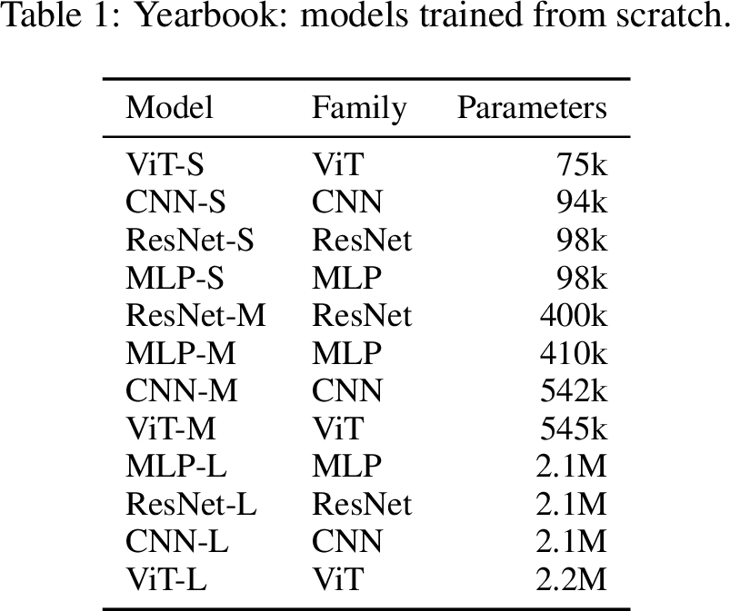 .
.
Figure 7: 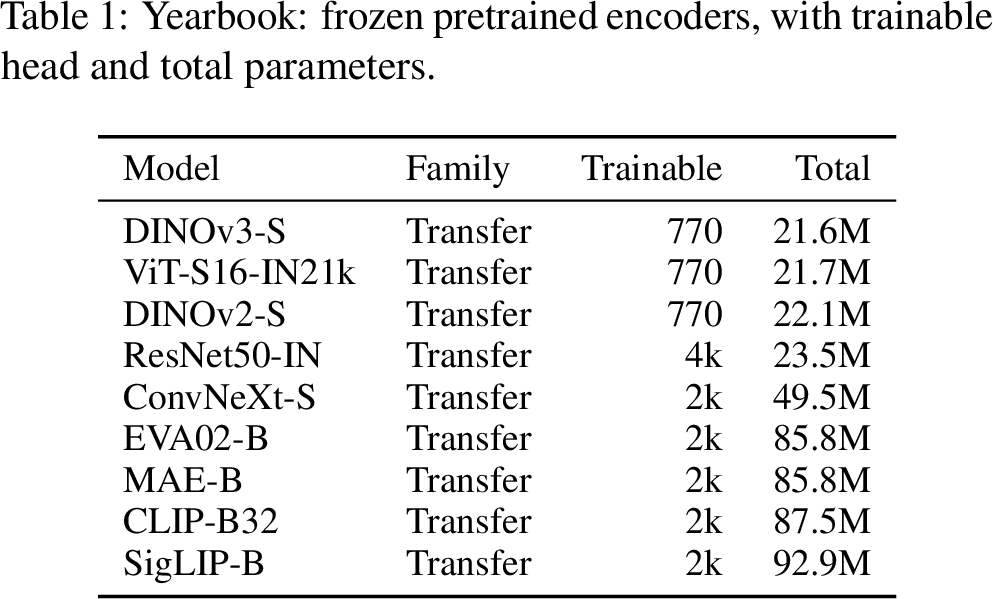 .
.
9.2 MLP↩︎

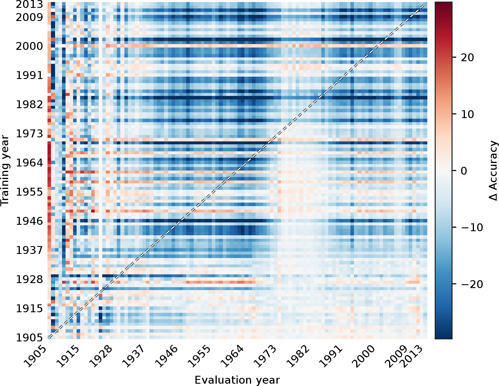

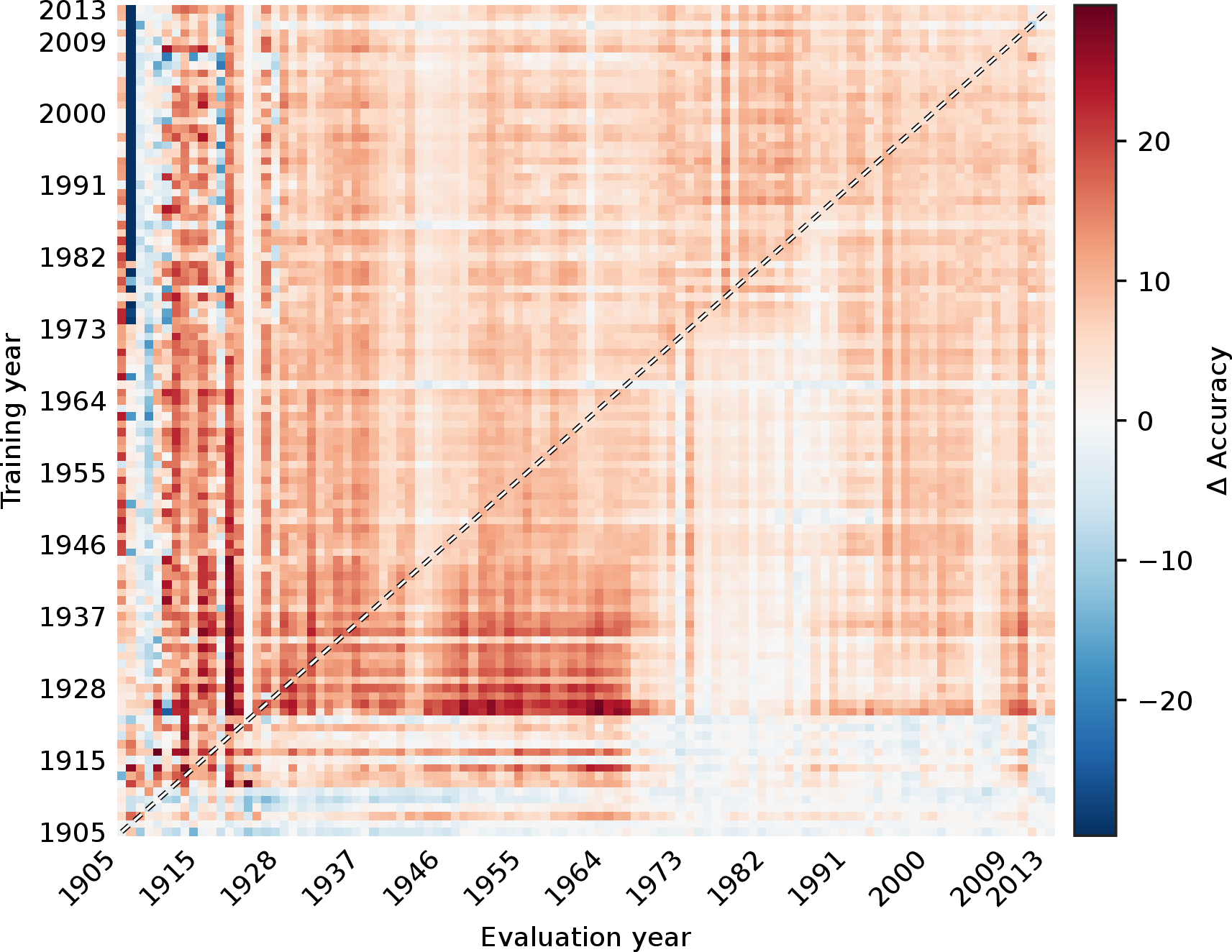


Figure 8: MLP models: Accuracy drift matrix \(M^{(m)}\) and deviation from the cohort mean \(\Delta^{(m)} = M^{(m)} - \bar{M}\) for each model, shown on a sequential and a zero-centred diverging scale, respectively.. b — MLP-S, d — MLP-M, f — MLP-L
9.3 CNN↩︎

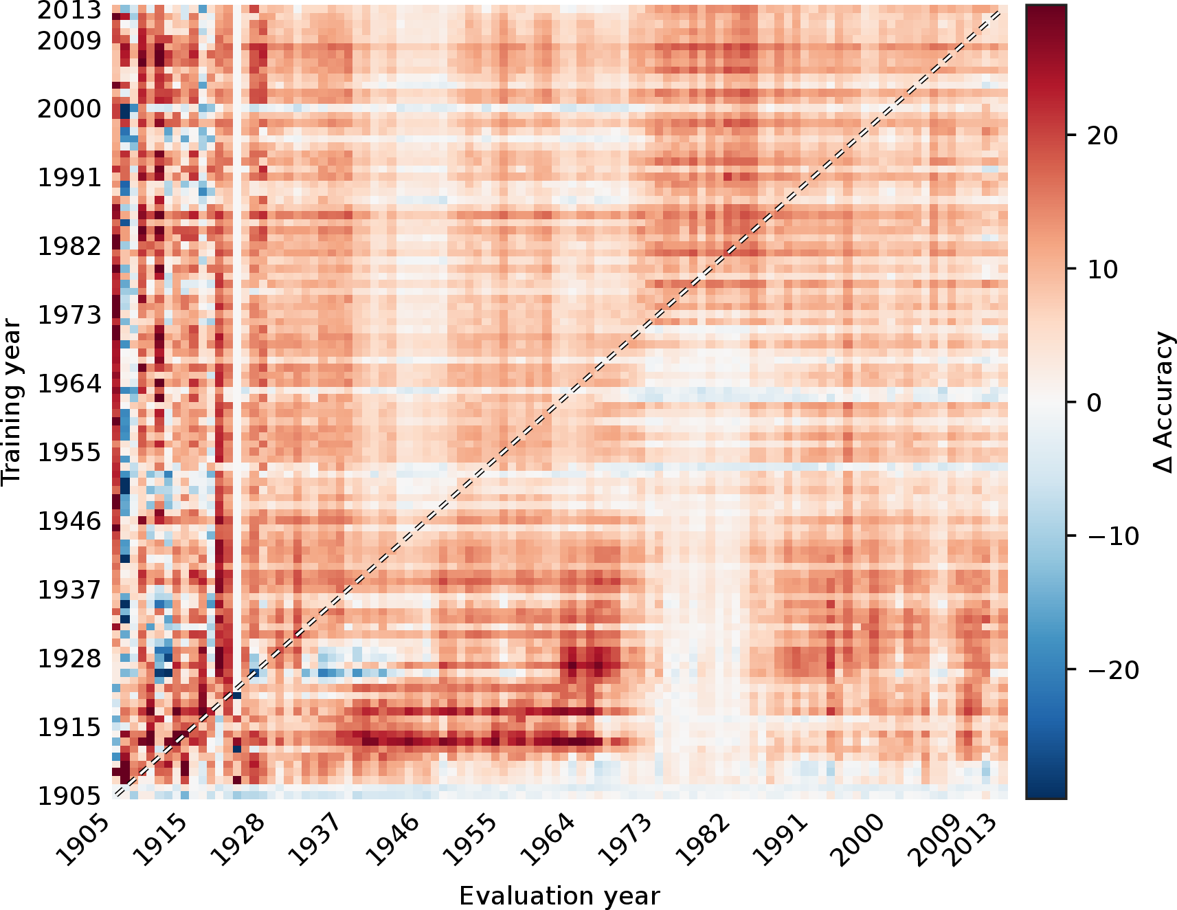

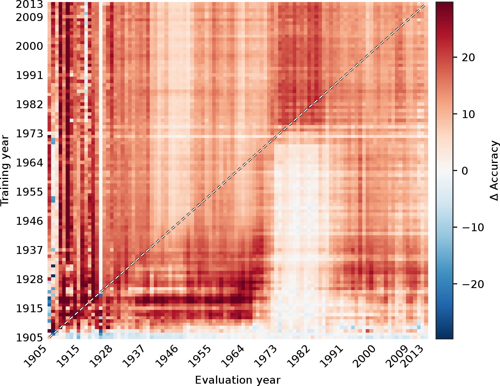

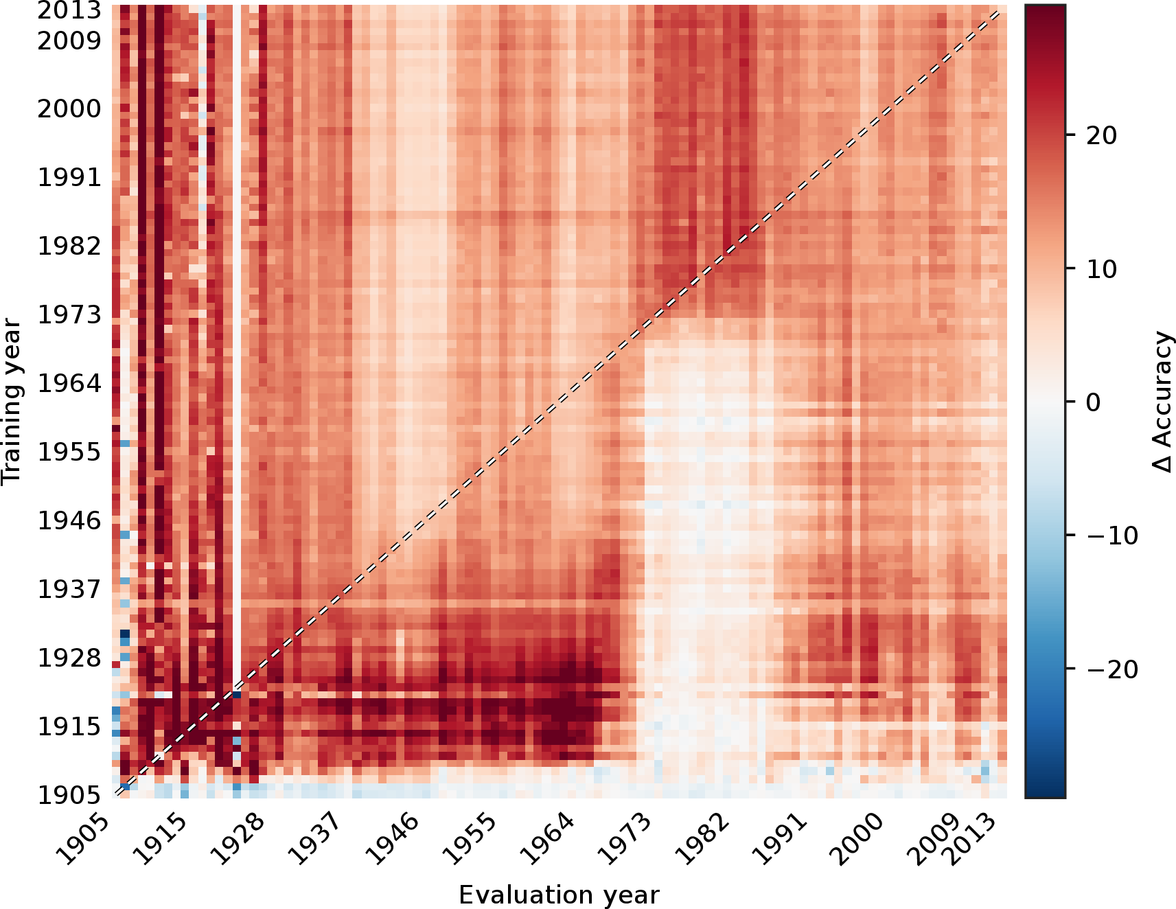
Figure 9: CNN models: Accuracy drift matrix \(M^{(m)}\) and deviation from the cohort mean \(\Delta^{(m)} = M^{(m)} - \bar{M}\) for each model, shown on a sequential and a zero-centred diverging scale, respectively.. b — CNN-S, d — CNN-M, f — CNN-L
9.4 ResNet↩︎

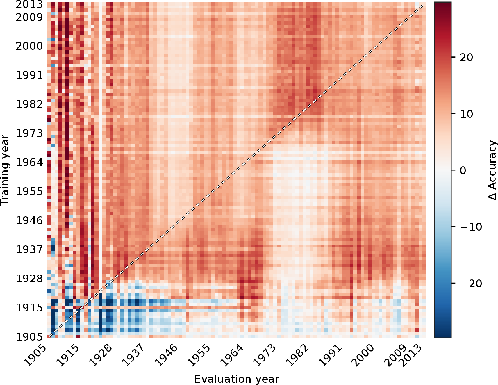

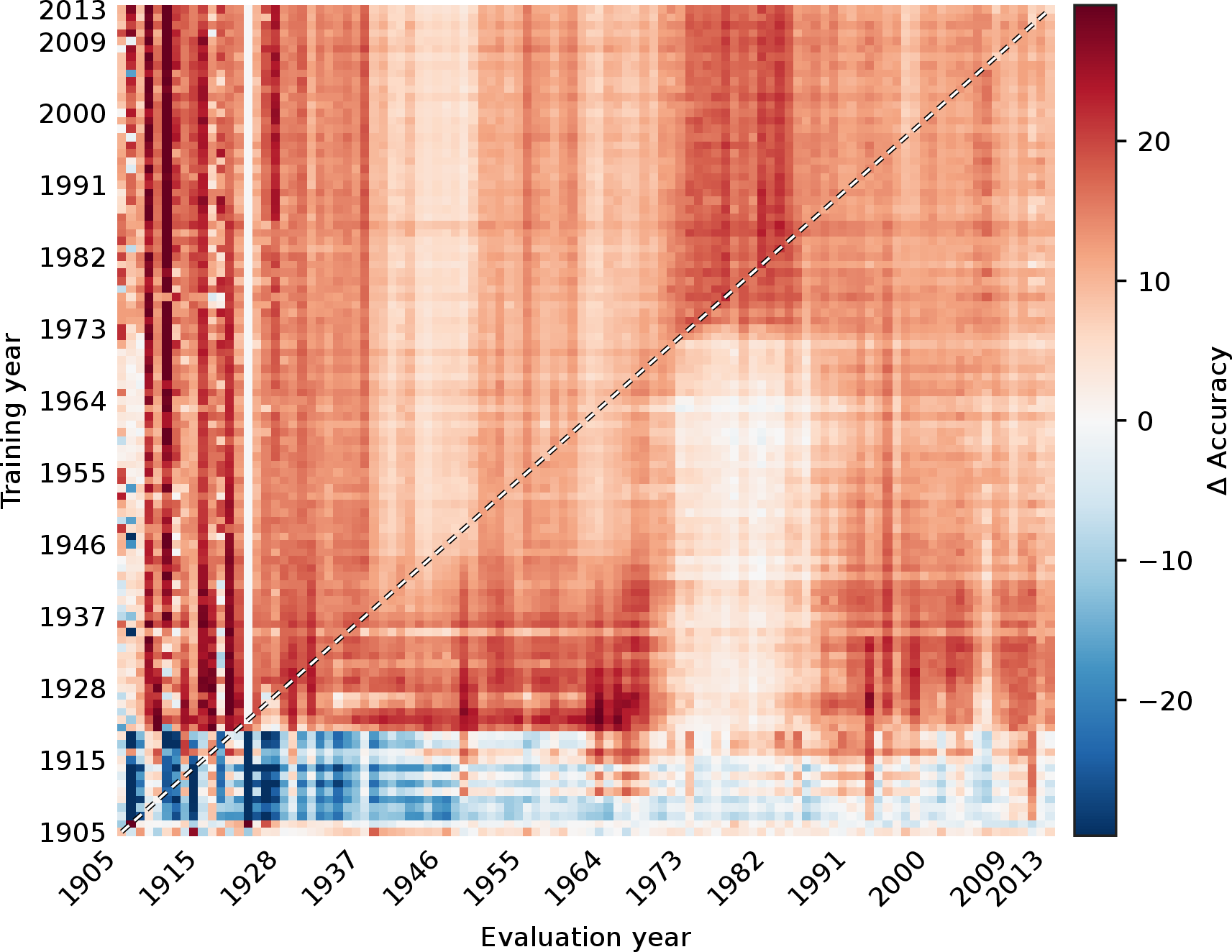

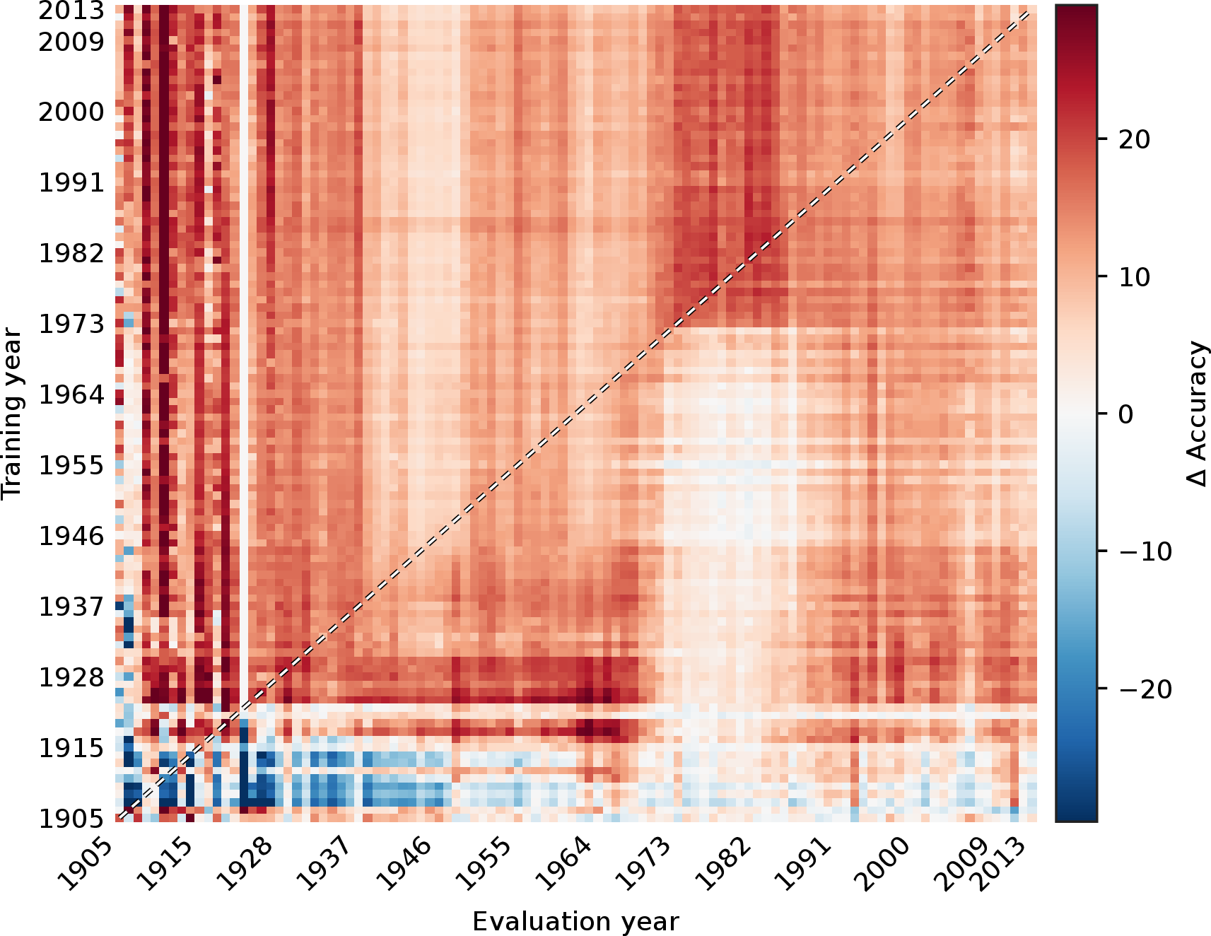
Figure 10: ResNet models: Accuracy drift matrix \(M^{(m)}\) and deviation from the cohort mean \(\Delta^{(m)} = M^{(m)} - \bar{M}\) for each model, shown on a sequential and a zero-centred diverging scale, respectively.. b — ResNet-S, d — ResNet-M, f — ResNet-L
9.5 ViT↩︎

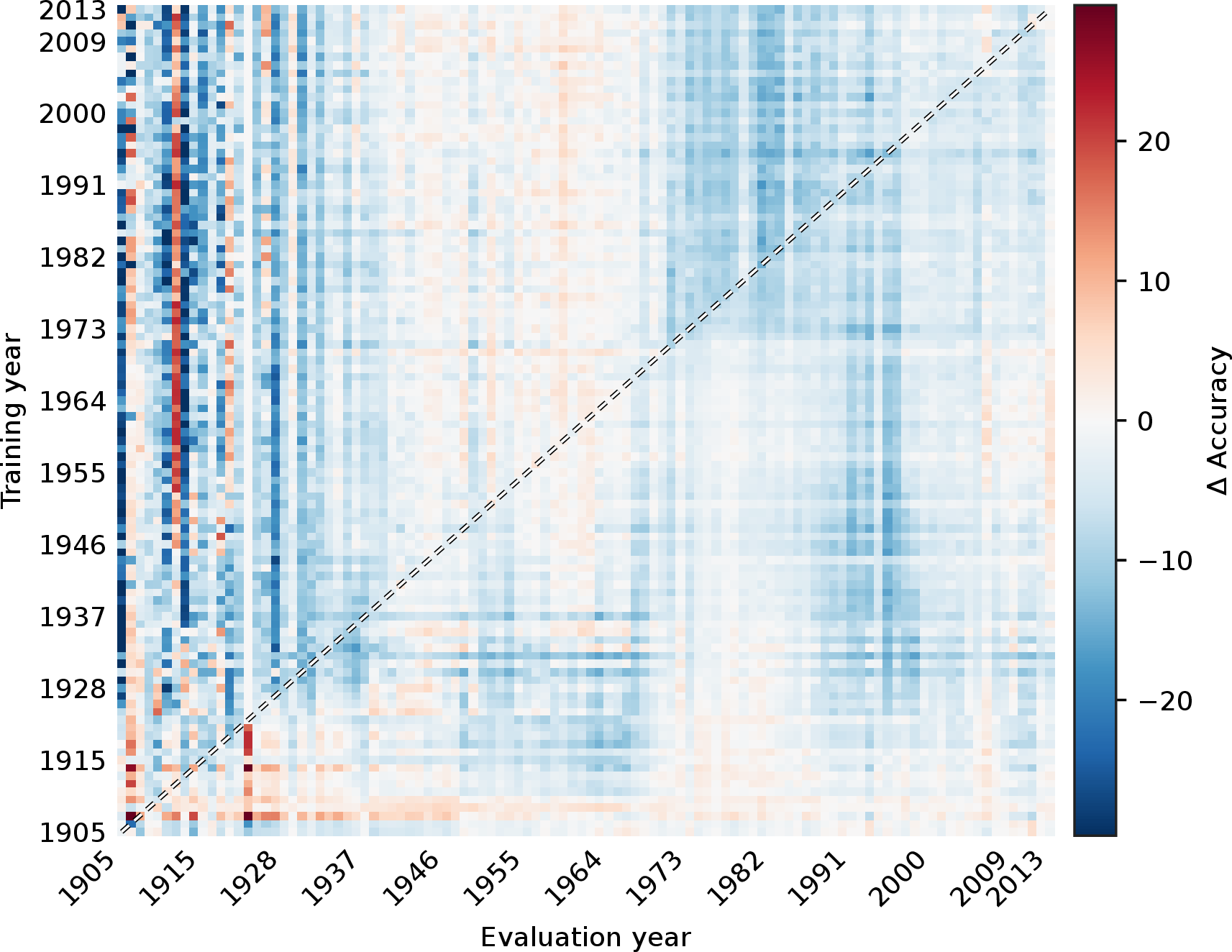

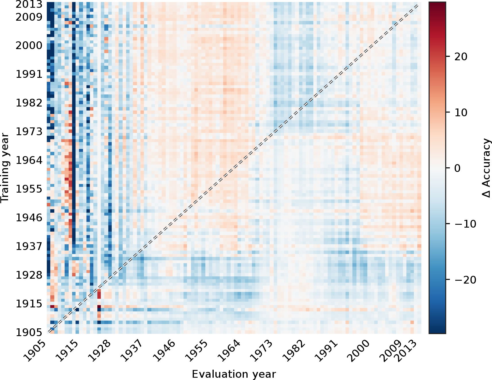

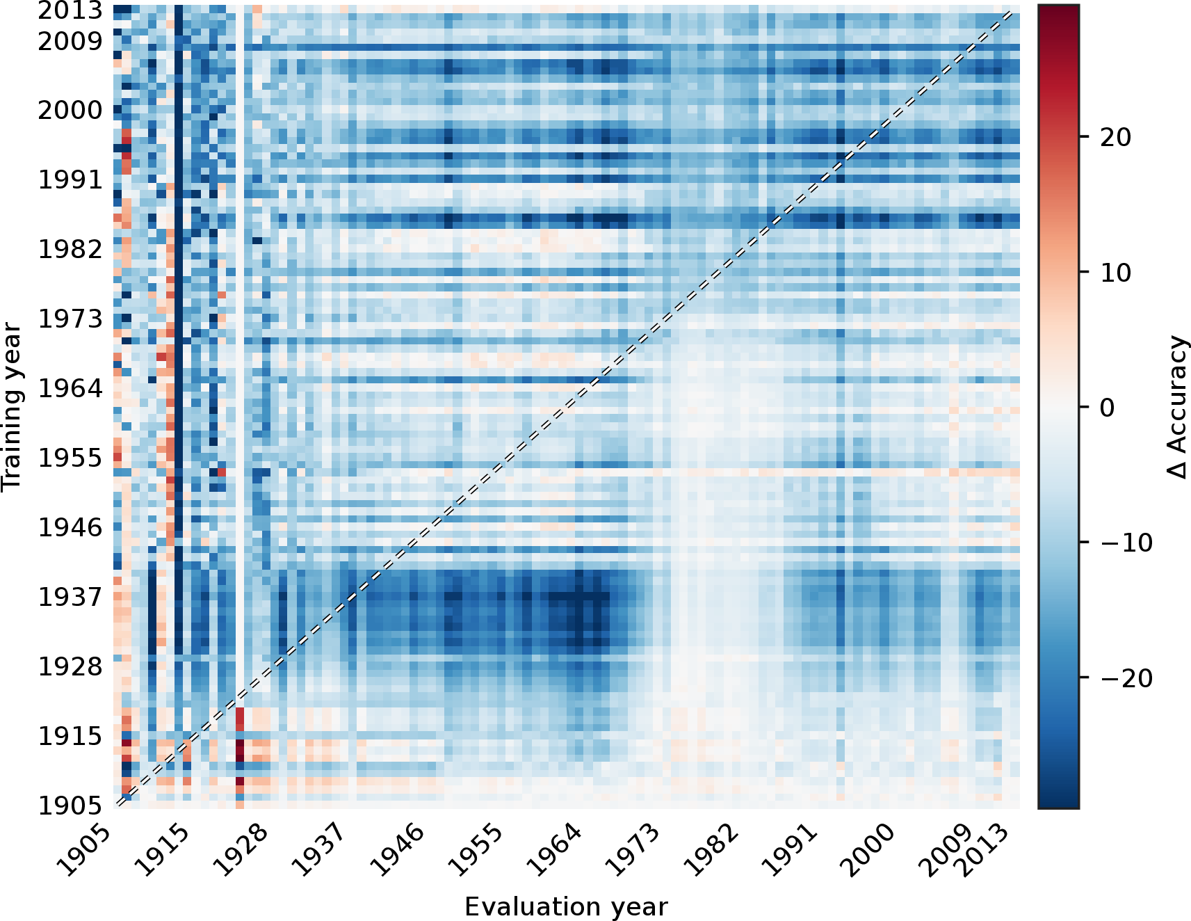
Figure 11: ViT models: Accuracy drift matrix \(M^{(m)}\) and deviation from the cohort mean \(\Delta^{(m)} = M^{(m)} - \bar{M}\) for each model, shown on a sequential and a zero-centred diverging scale, respectively.. b — ViT-S, d — ViT-M, f — ViT-L
9.6 Transfer↩︎

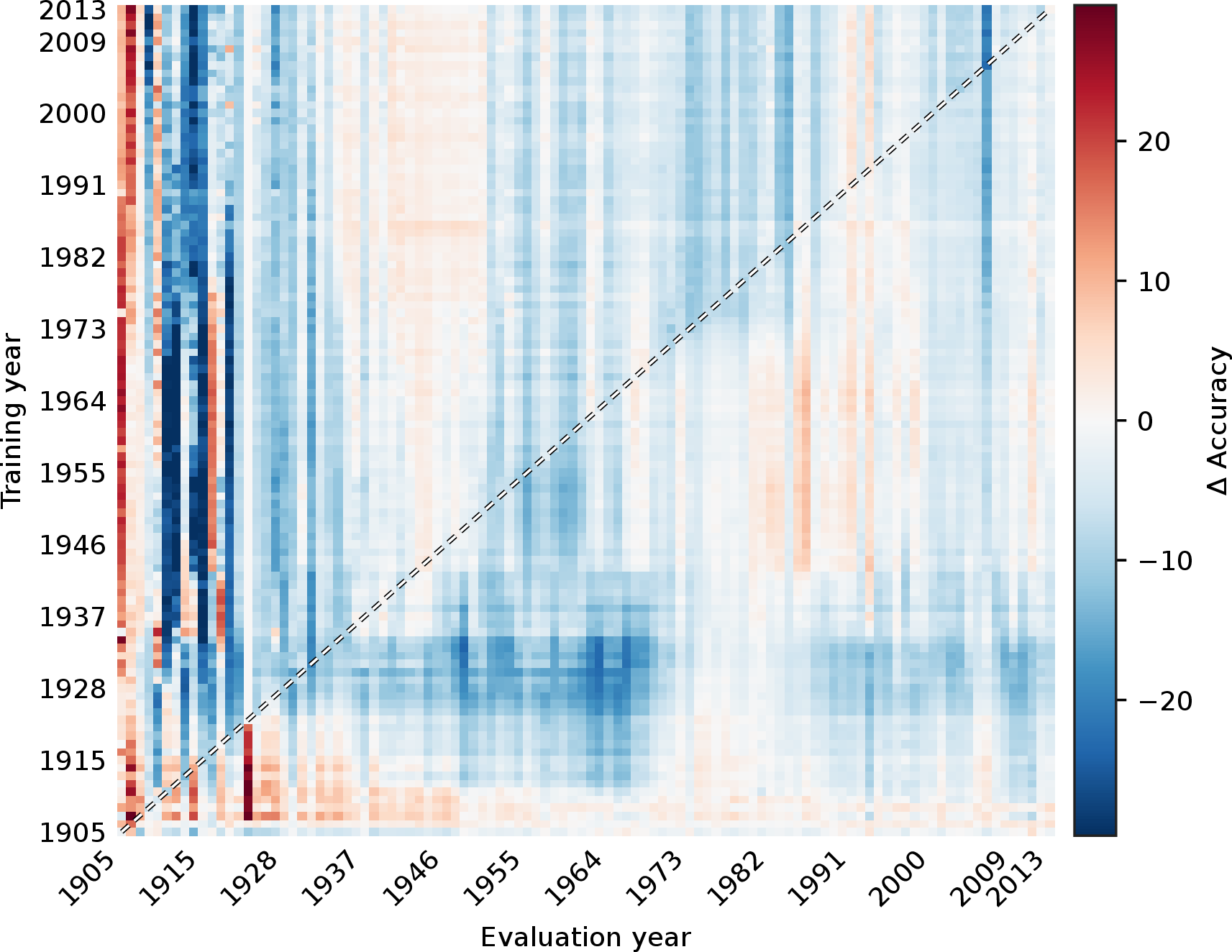

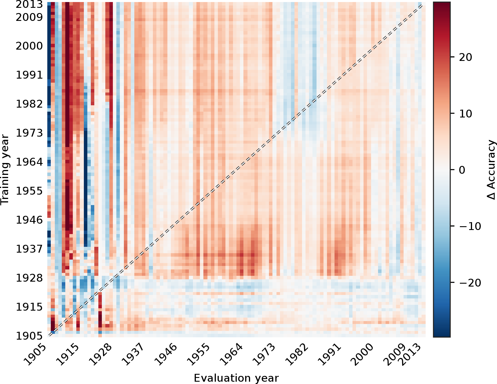

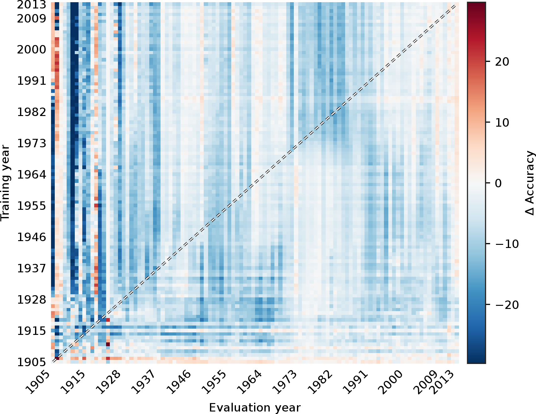

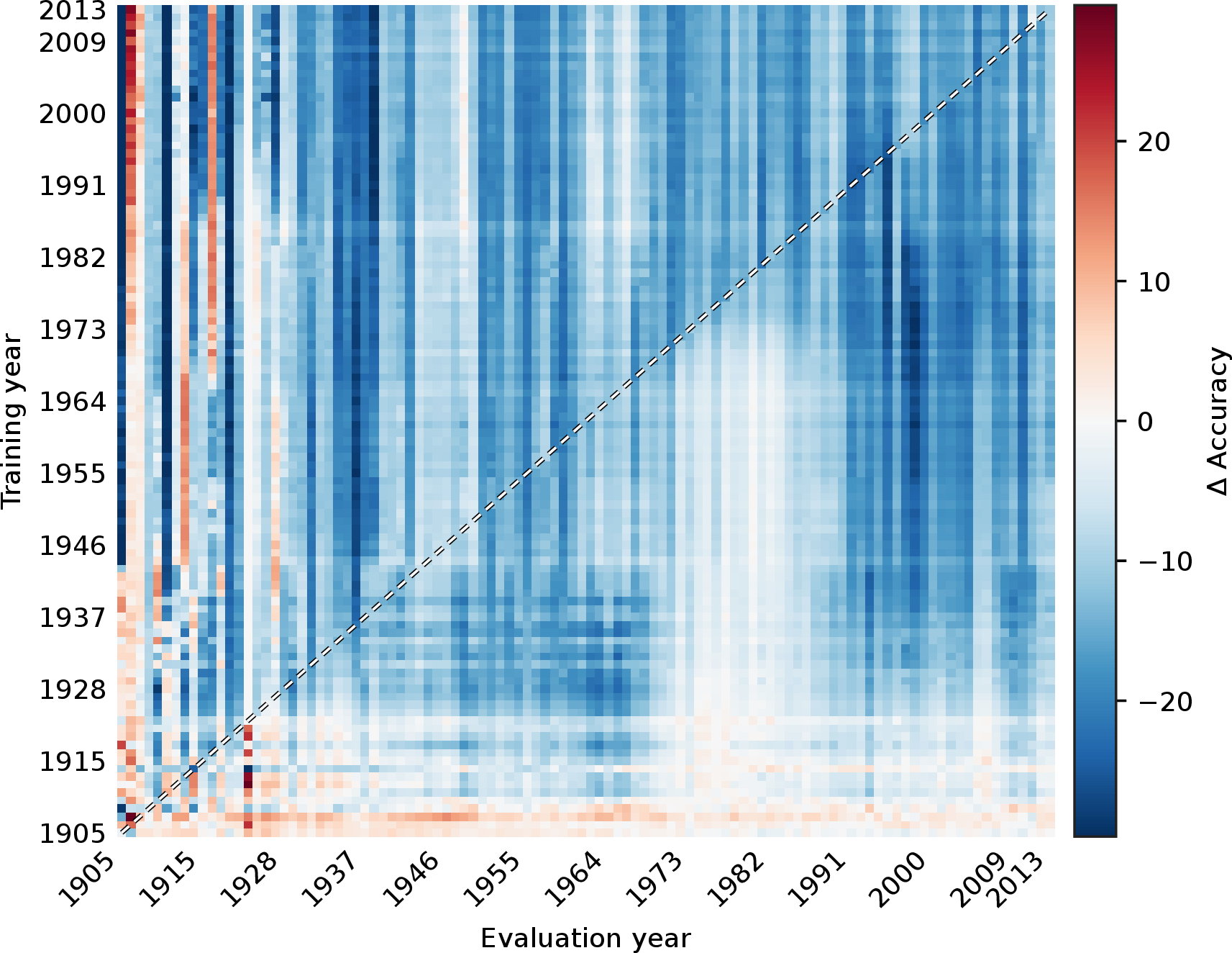

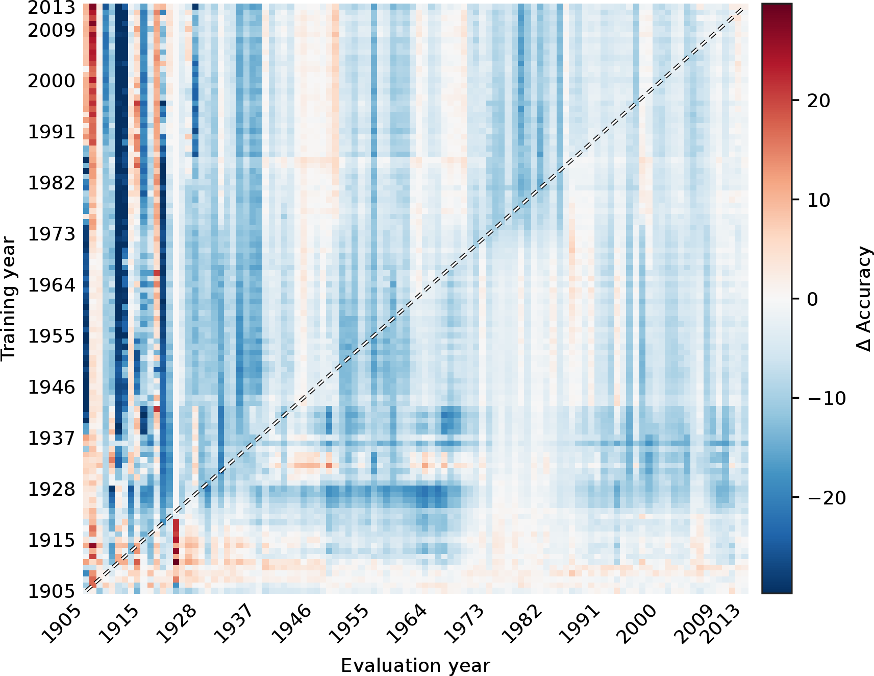

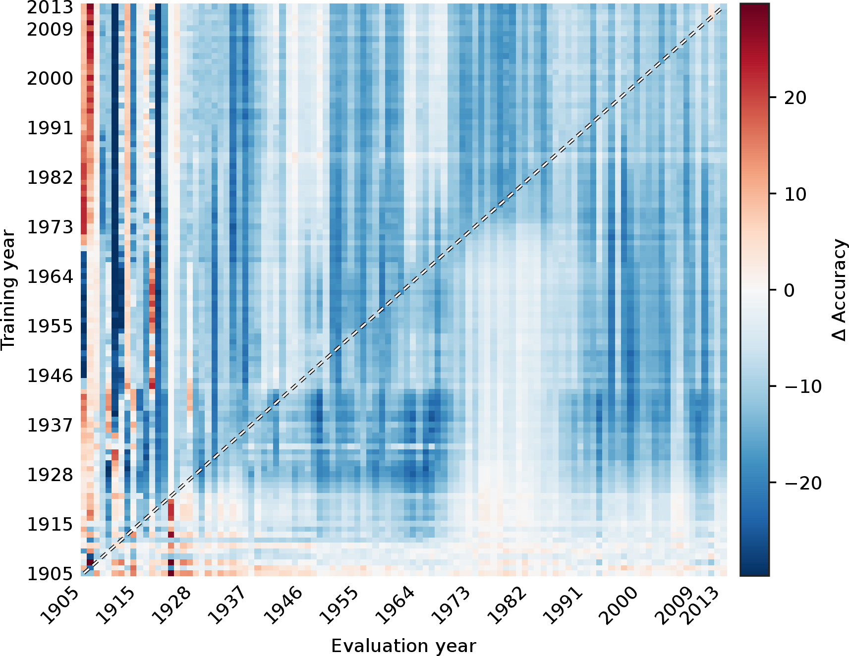


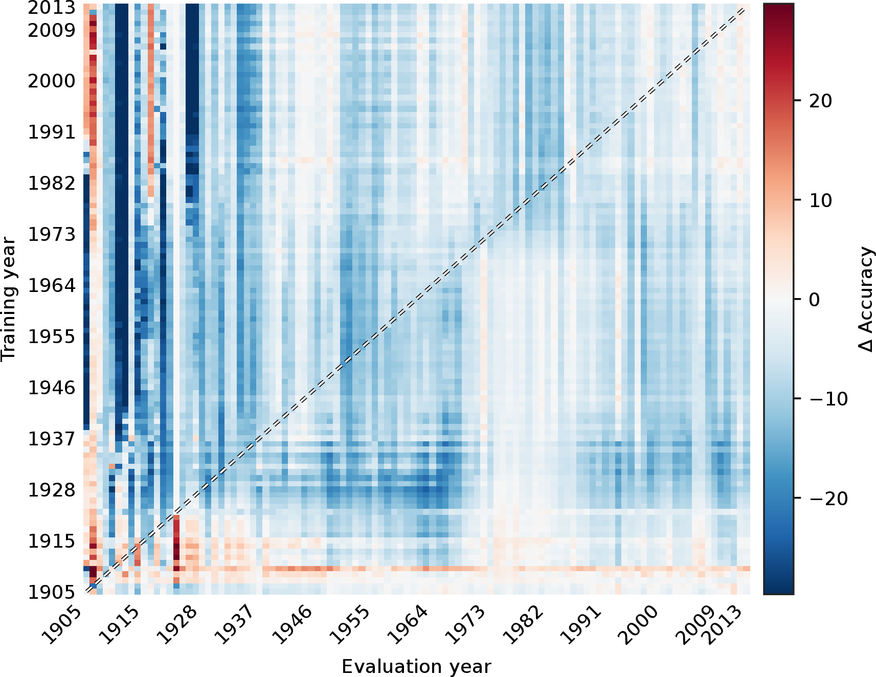

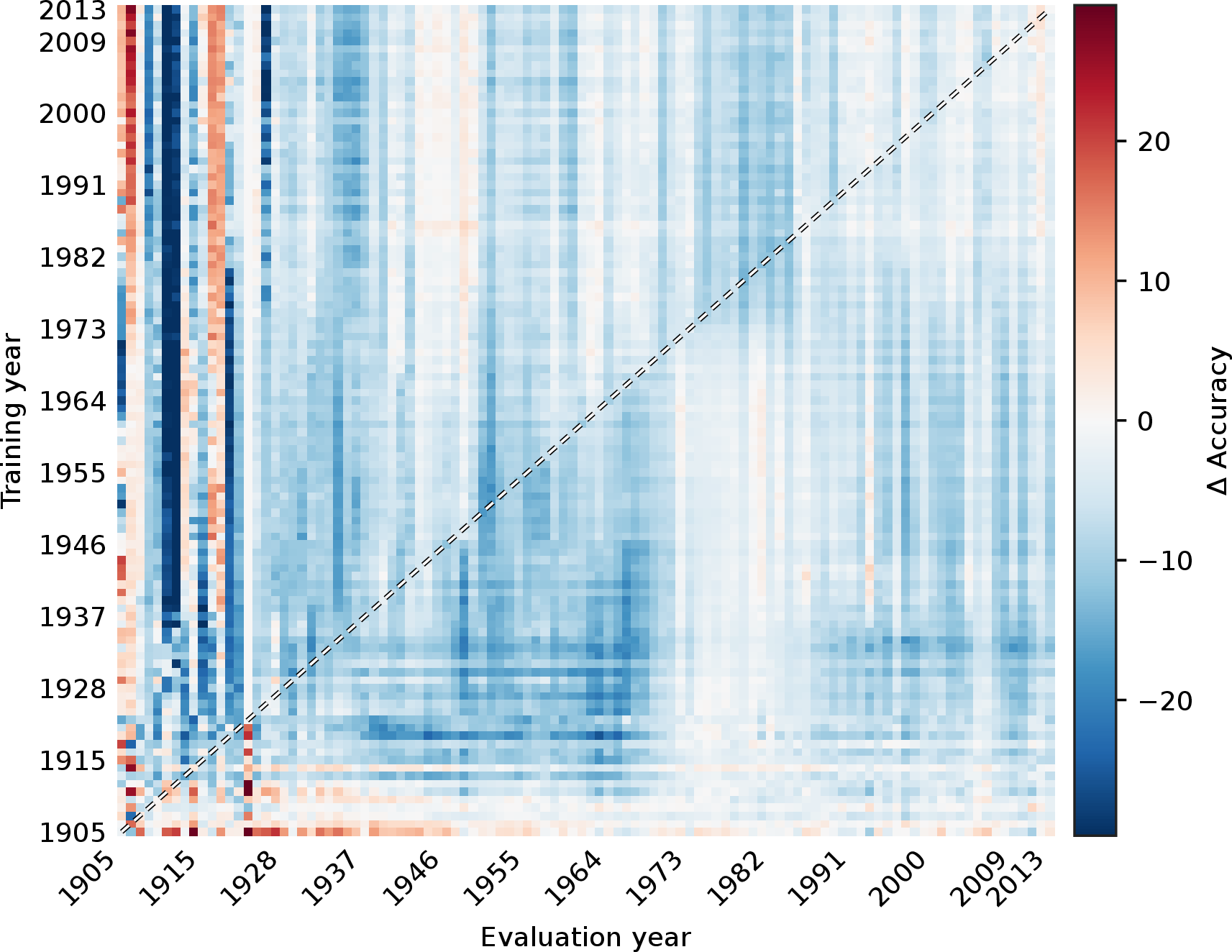
Figure 12: Transfer models: Accuracy drift matrix \(M^{(m)}\) and deviation from the cohort mean \(\Delta^{(m)} = M^{(m)} - \bar{M}\) for each model, shown on a sequential and a zero-centred diverging scale, respectively.. b — CLIP-B32, d — ConvNeXt-S, f — DINOv2-S, h — DINOv3-S, j — EVA02-B, l — MAE-B, n — ResNet50-IN, p — SigLIP-B, r — ViT-S16-IN21k
9.7 Forgetting and Rankings↩︎
To see how quickly each model forgets, we summarize its drift matrix as a forgetting curve. The curve plots the Accuracy against the lag \(\ell = j - i\), the number of slices between the training cutoff \(i\) and the evaluation slice \(j\). At each lag we average over all training cutoffs, \[F(\ell) = \operatorname{mean}_{i} M_{i,\,i+\ell}.\] The result is the Accuracy at a fixed temporal distance, independent of which period a model was trained on. This separates the effect of temporal distance from the difficulty of any single slice.
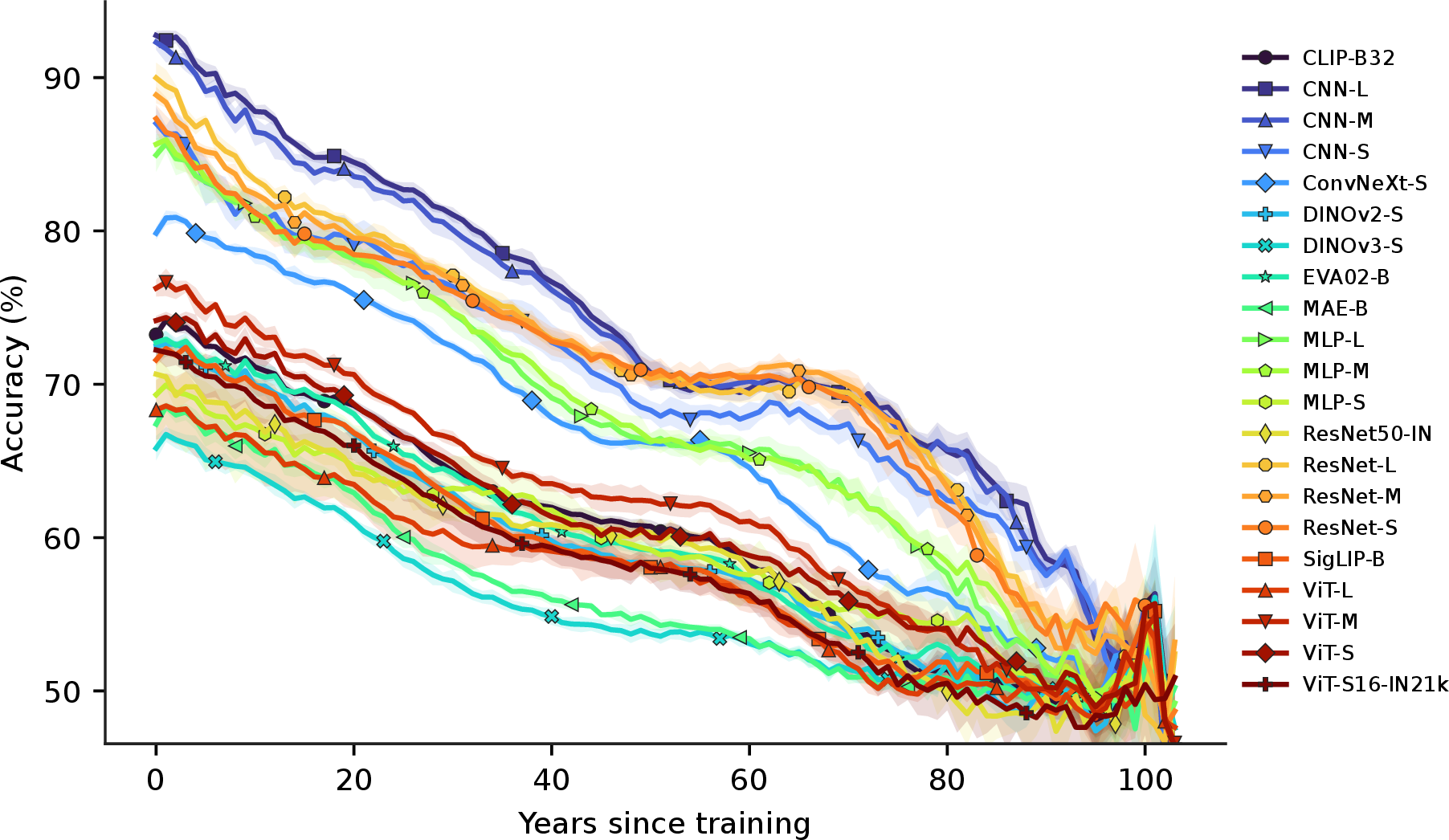
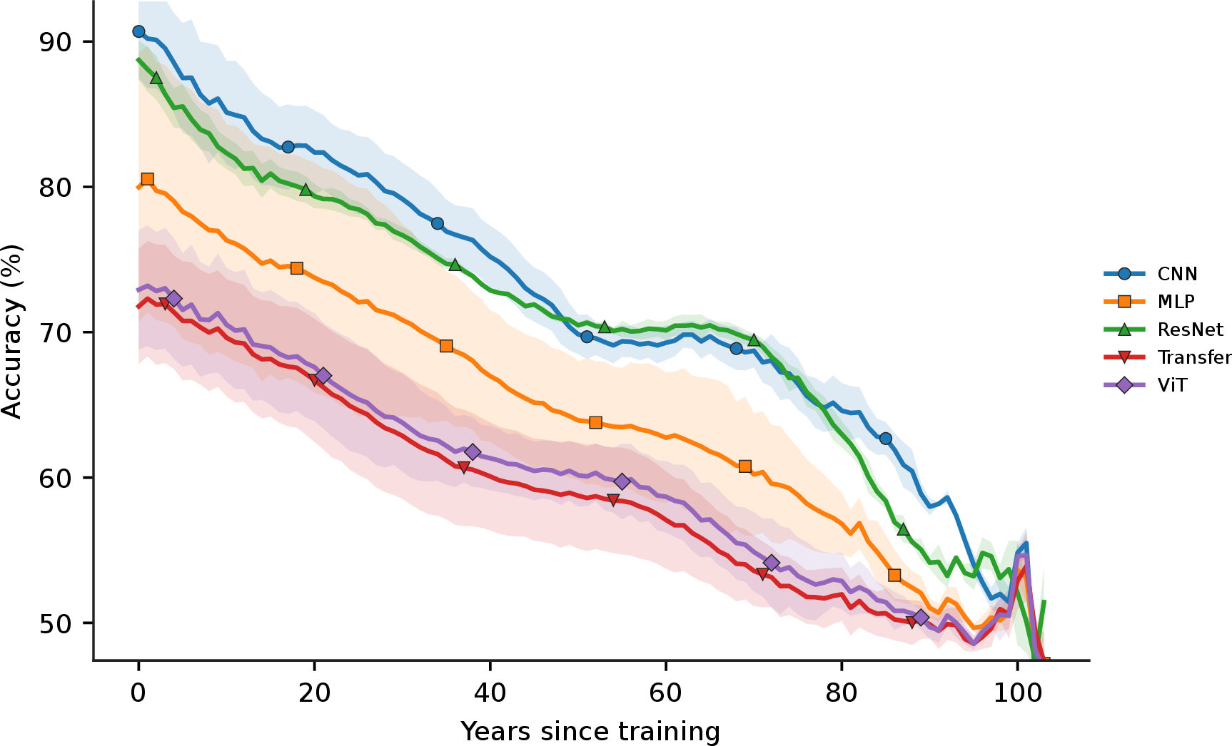
Figure 13: Forgetting curves: each model (left) and averaged within each family (right).. a — Per model, b — Per model family


Figure 14: Models ranked by mean future performance and by temporal decay.. a — By future performance, b — By decay
9.8 Result Tables↩︎
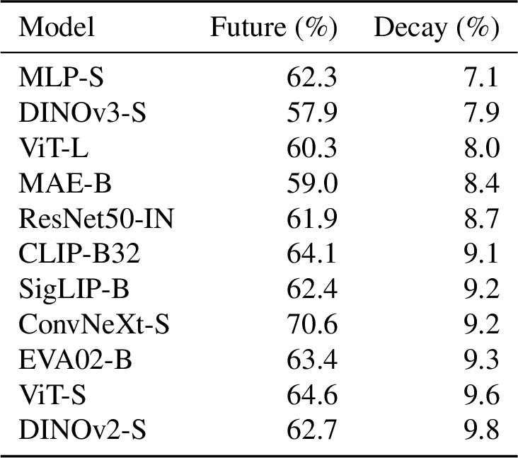
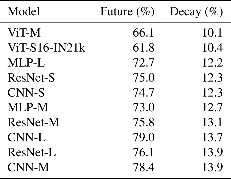
Figure 15: 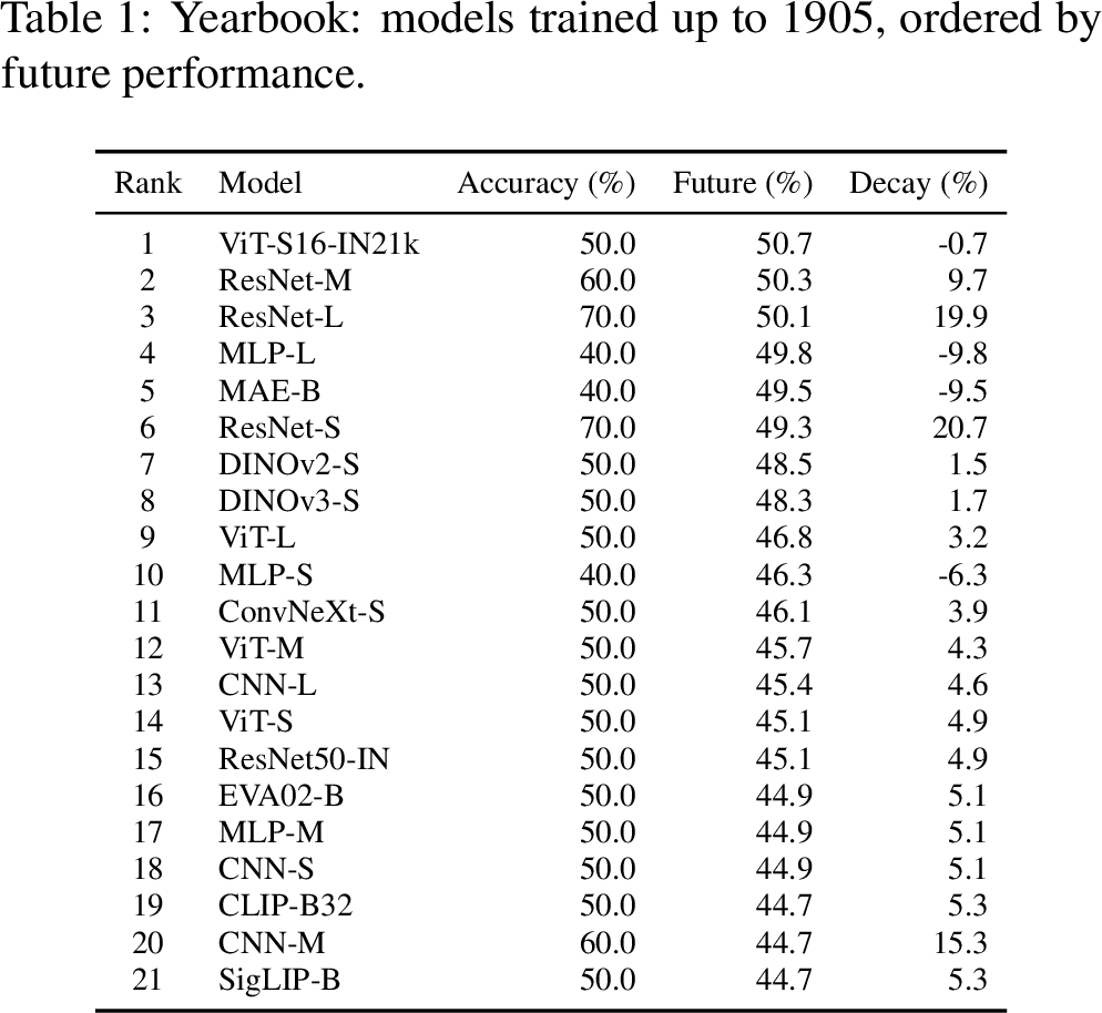 .
.
Figure 16: 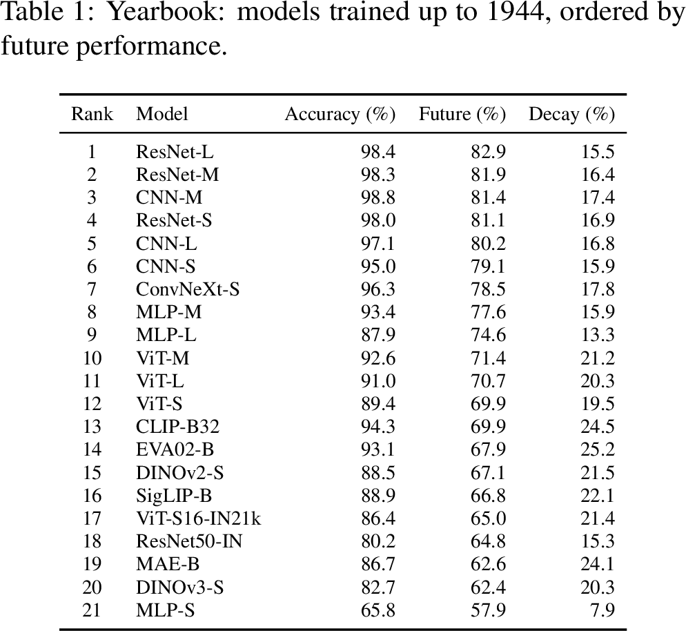 .
.
Figure 17: 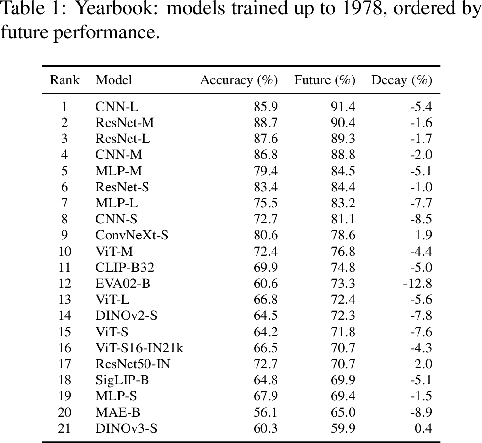 .
.
Figure 18: 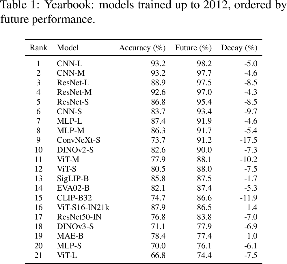 .
.
| 1905 | 1944 | 1978 | 2012 | |||||
| Family | Future | Decay | Future | Decay | Future | Decay | Future | Decay |
| CNN | 45.0 | 8.3 | 80.3 | 16.7 | 87.1 | -5.3 | 96.4 | -6.4 |
| MLP | 47.0 | -3.7 | 70.0 | 12.4 | 79.0 | -4.8 | 86.6 | -5.3 |
| ResNet | 49.9 | 16.8 | 82.0 | 16.2 | 88.0 | -1.4 | 96.6 | -7.1 |
| Transfer | 46.9 | 1.9 | 67.2 | 21.4 | 70.6 | -4.4 | 85.4 | -6.1 |
| ViT | 45.9 | 4.1 | 70.7 | 20.3 | 73.7 | -5.9 | 83.5 | -8.4 |
10 Amazon Reviews – Drift Matrices↩︎
The cohort-mean and per-model deviation matrices shown here, and the in-distribution, future, and decay quantities tabulated below, are defined in Section 4.5.
10.1 Model Roster↩︎
Figure 20: 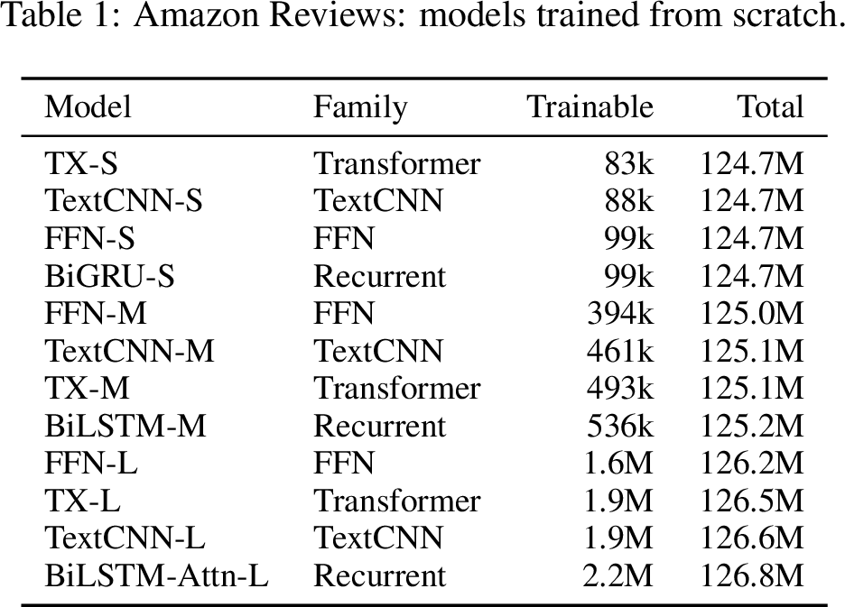 .
.
Figure 21: 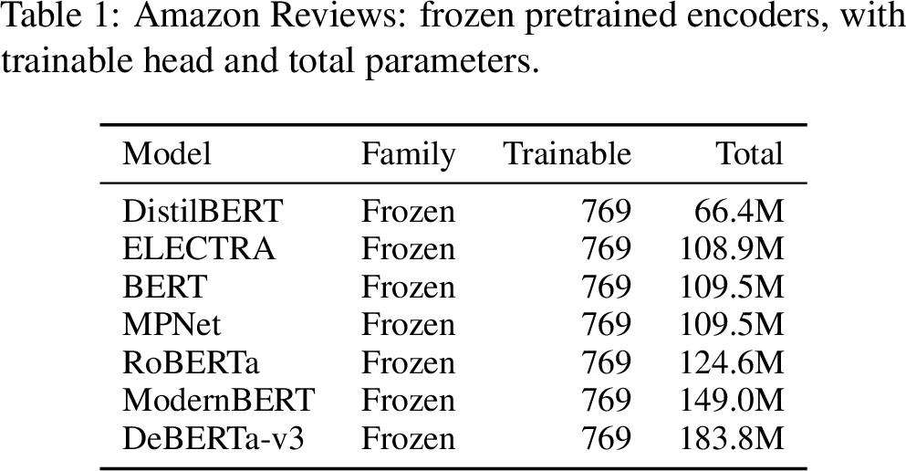 .
.
10.2 FFN↩︎

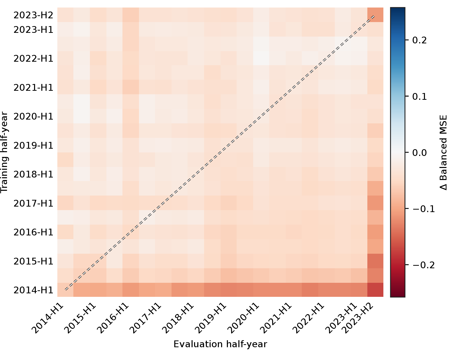

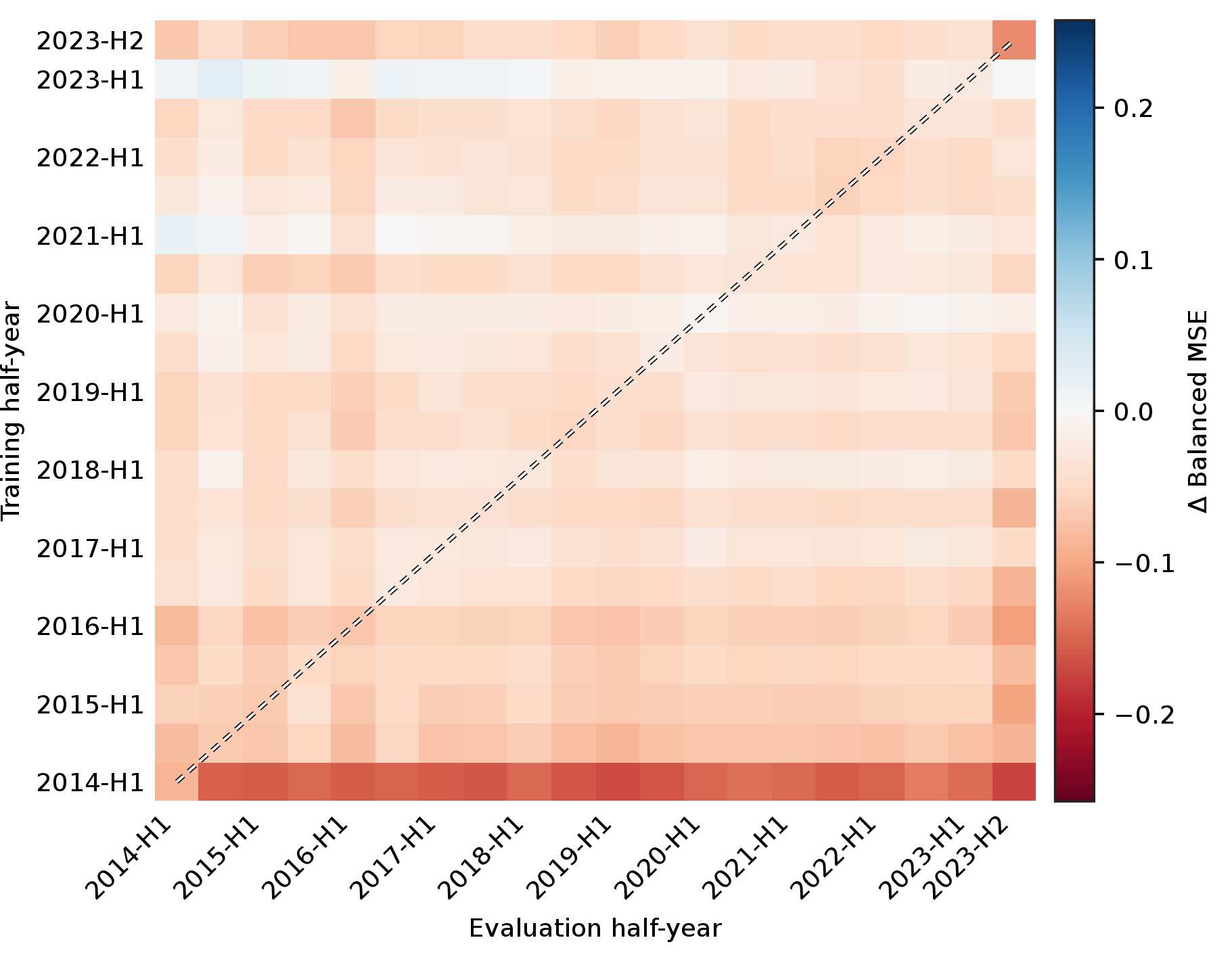

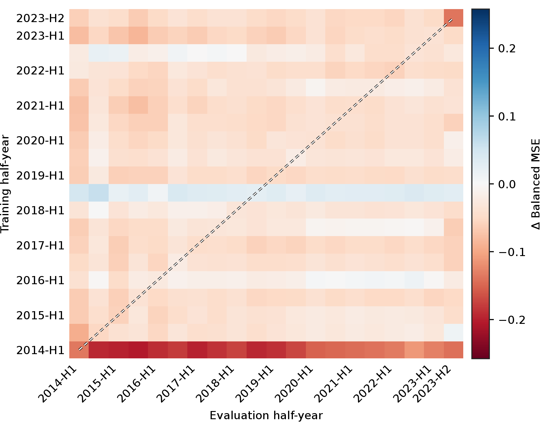
Figure 22: FFN models: Balanced MSE drift matrix \(M^{(m)}\) and deviation from the cohort mean \(\Delta^{(m)} = M^{(m)} - \bar{M}\) for each model, shown on a sequential and a zero-centred diverging scale, respectively.. b — FFN-S, d — FFN-M, f — FFN-L
10.3 TextCNN↩︎

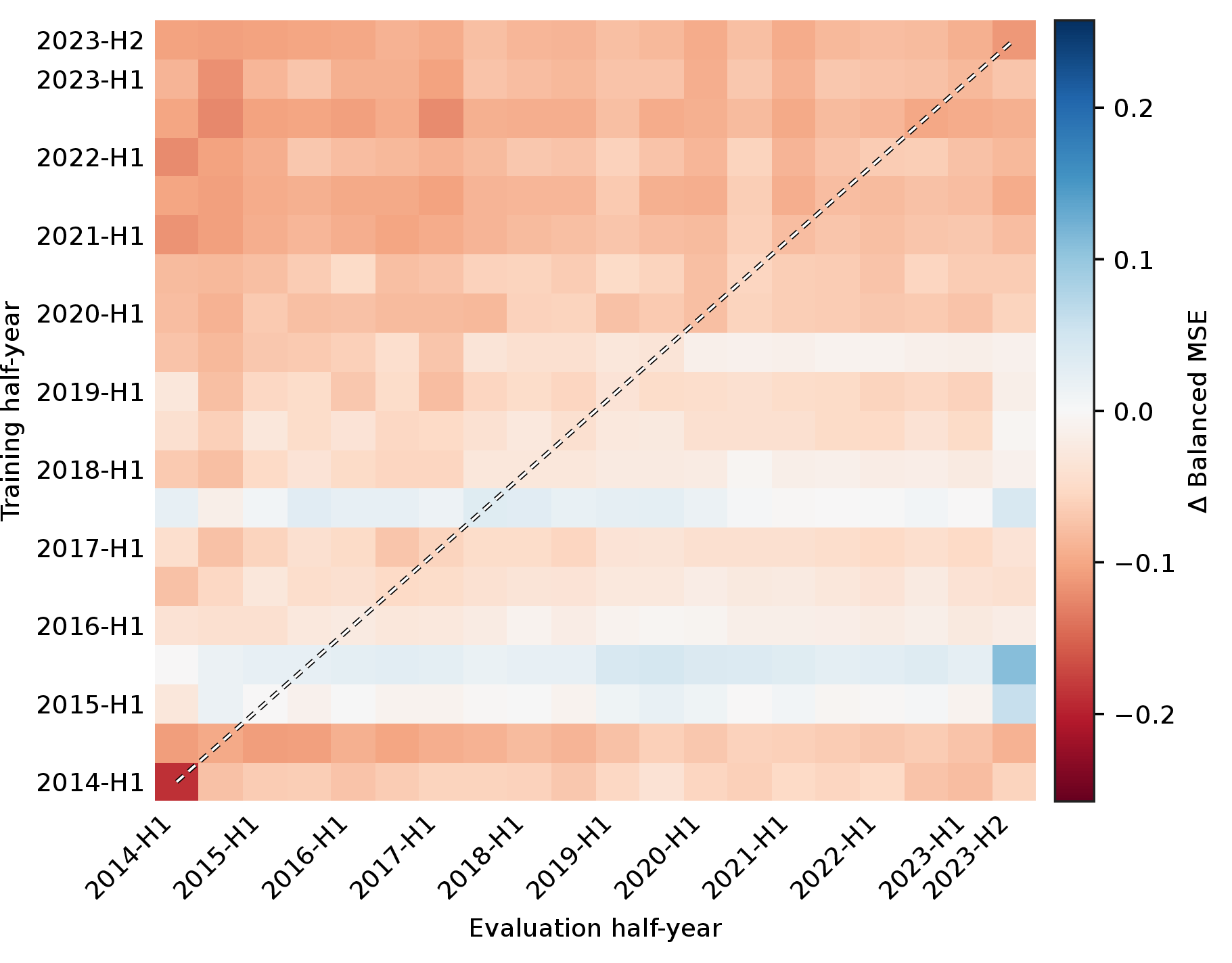

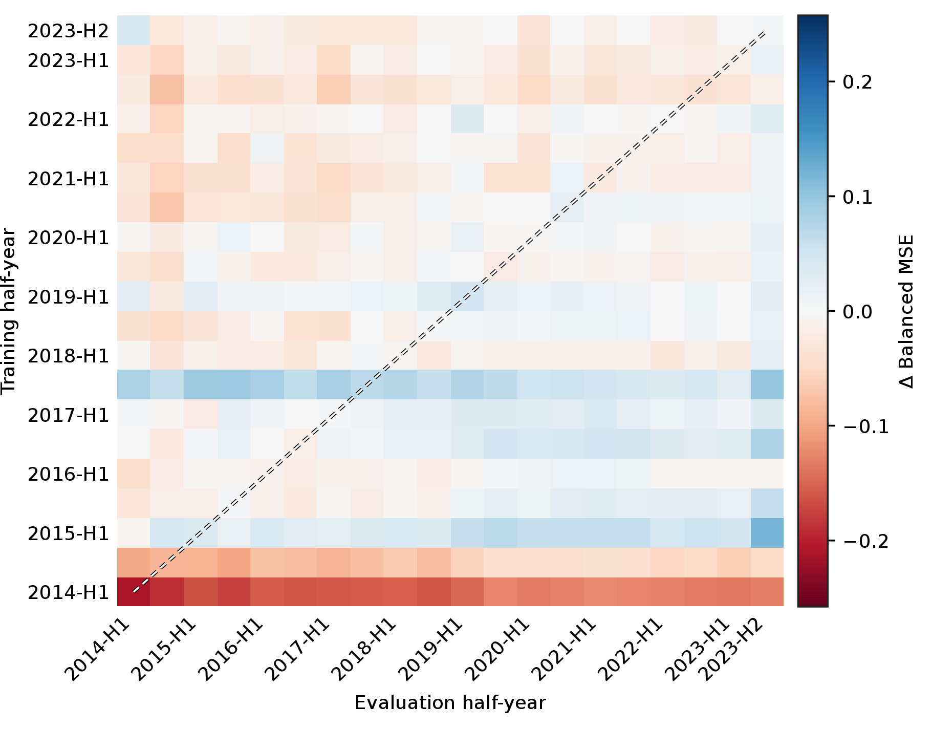

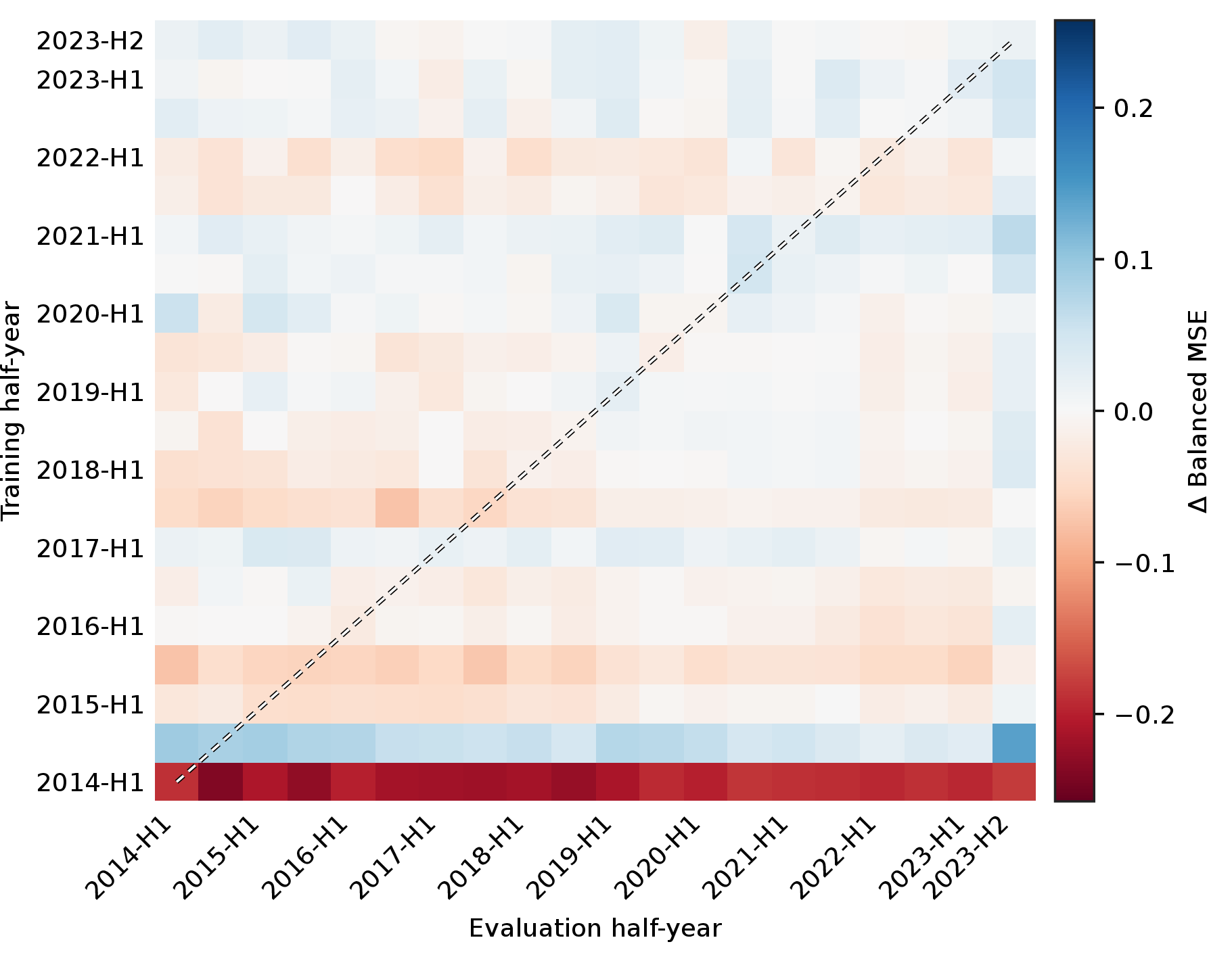
Figure 23: TextCNN models: Balanced MSE drift matrix \(M^{(m)}\) and deviation from the cohort mean \(\Delta^{(m)} = M^{(m)} - \bar{M}\) for each model, shown on a sequential and a zero-centred diverging scale, respectively.. b — TextCNN-S, d — TextCNN-M, f — TextCNN-L
10.4 Recurrent↩︎

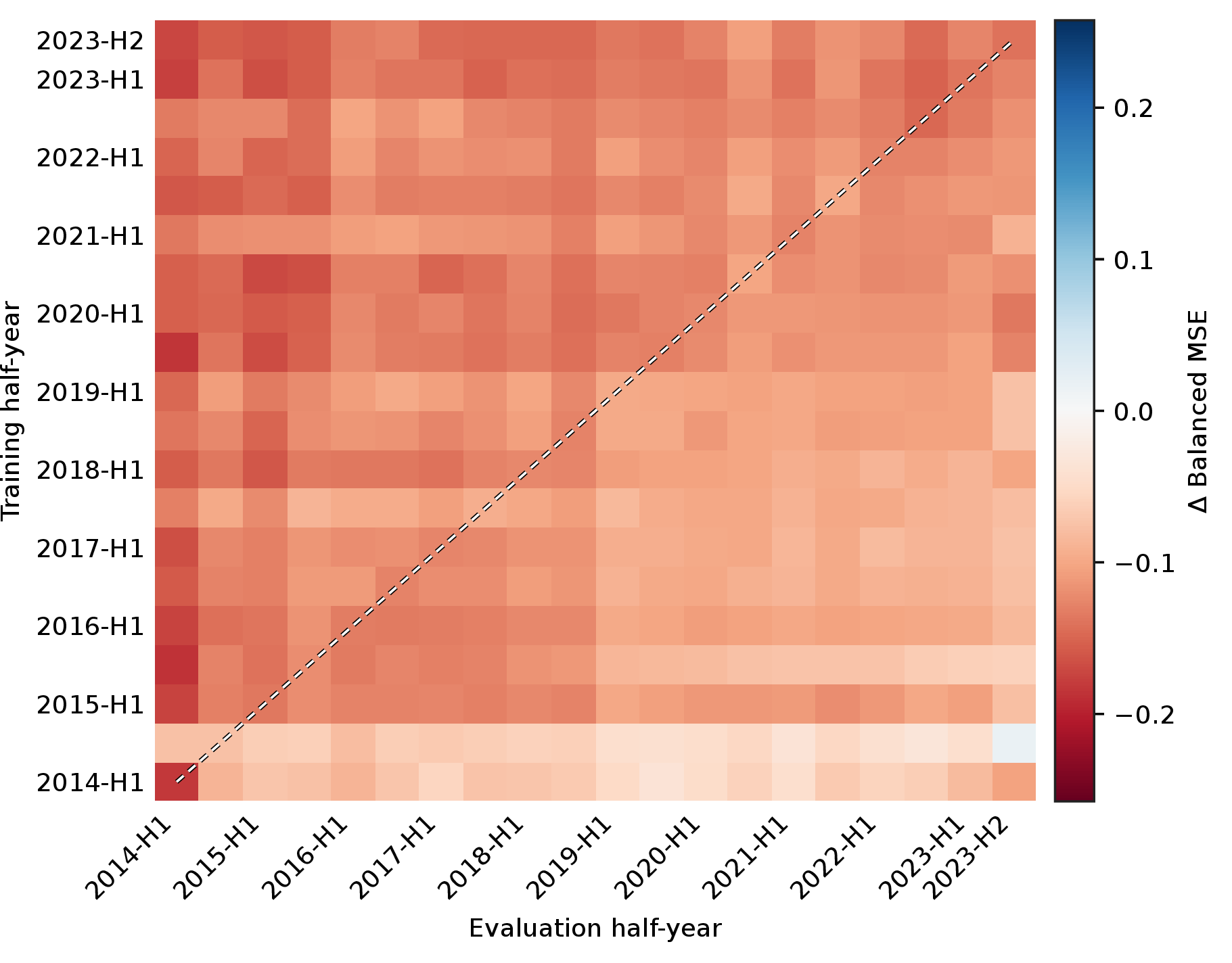

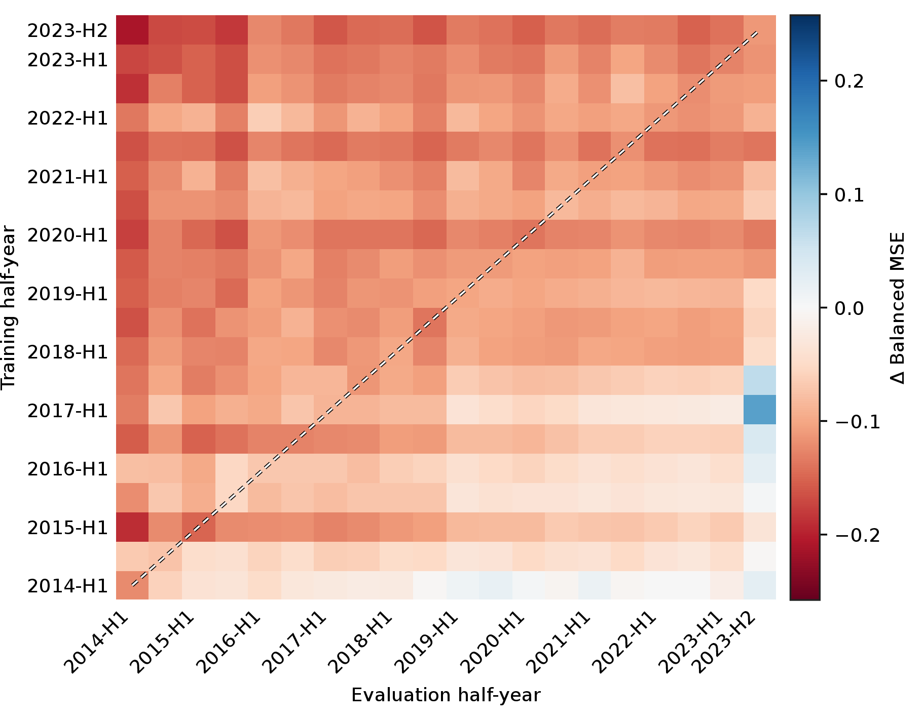

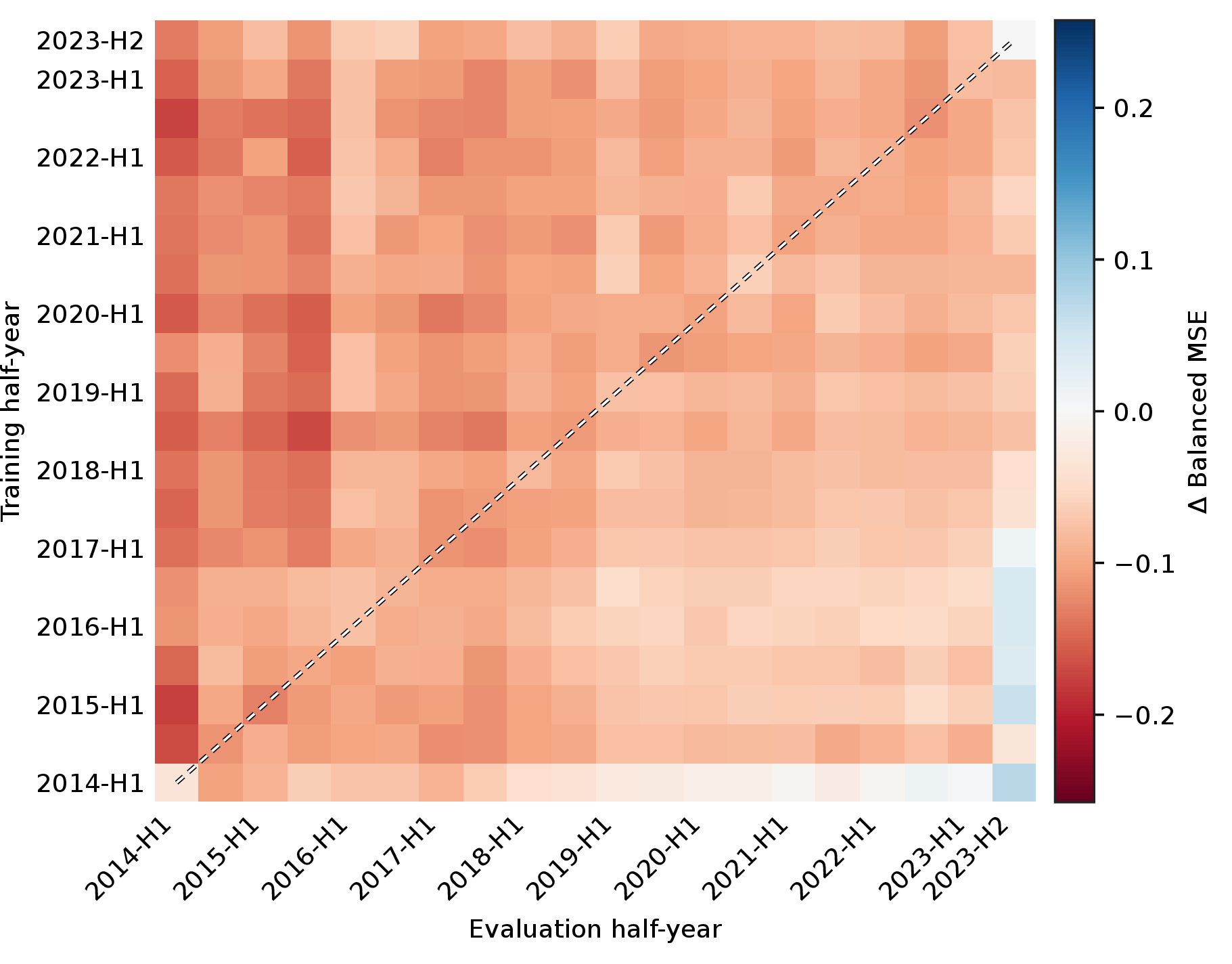
Figure 24: Recurrent models: Balanced MSE drift matrix \(M^{(m)}\) and deviation from the cohort mean \(\Delta^{(m)} = M^{(m)} - \bar{M}\) for each model, shown on a sequential and a zero-centred diverging scale, respectively.. b — BiGRU-S, d — BiLSTM-M, f — BiLSTM-Attn-L
10.5 Transformer↩︎

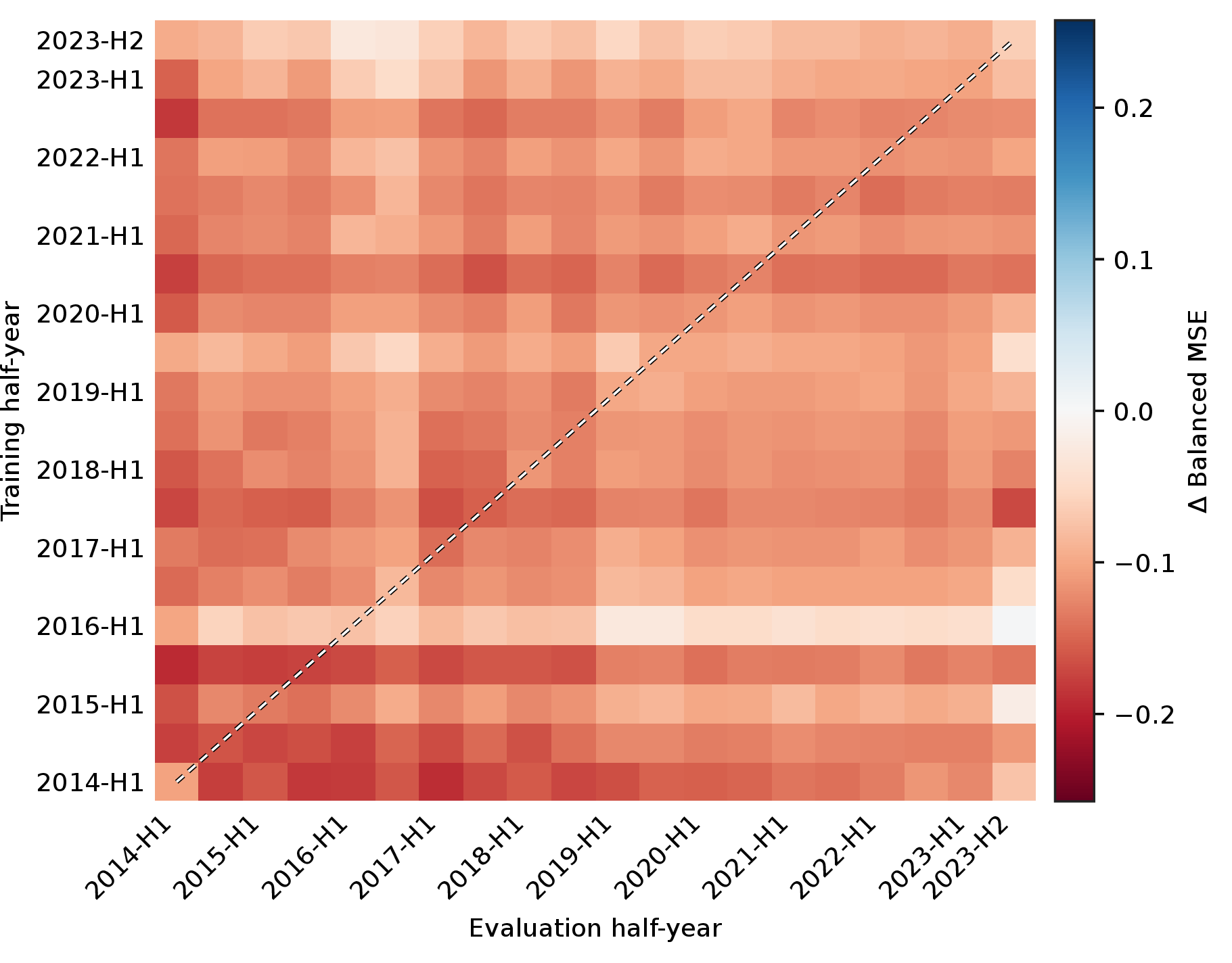

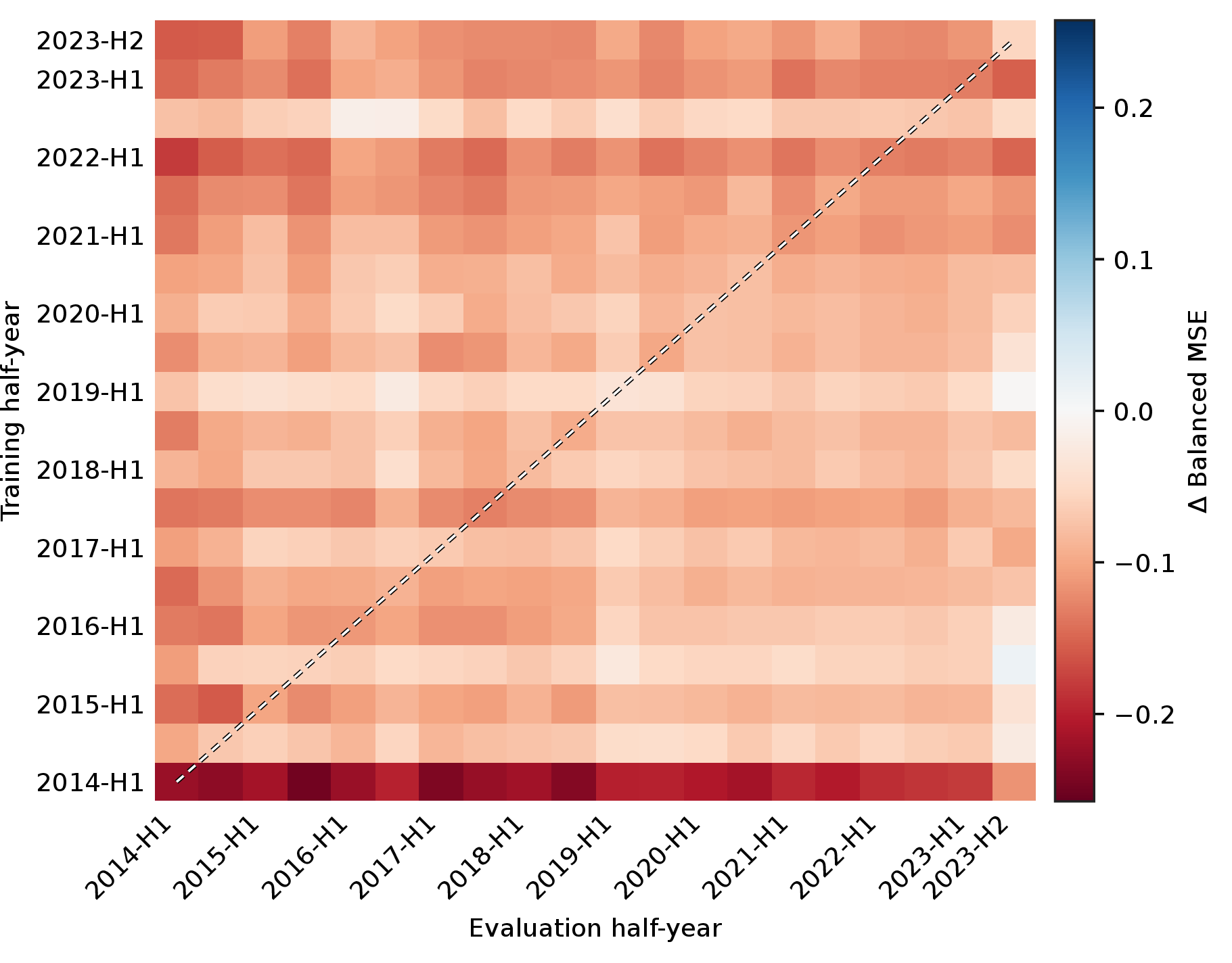


Figure 25: Transformer models: Balanced MSE drift matrix \(M^{(m)}\) and deviation from the cohort mean \(\Delta^{(m)} = M^{(m)} - \bar{M}\) for each model, shown on a sequential and a zero-centred diverging scale, respectively.. b — TX-S, d — TX-M, f — TX-L
10.6 Frozen↩︎

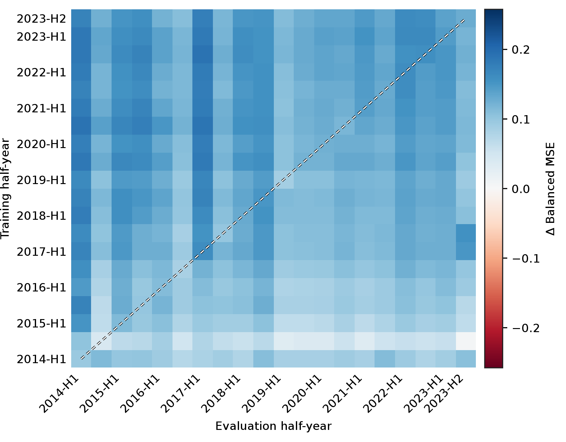

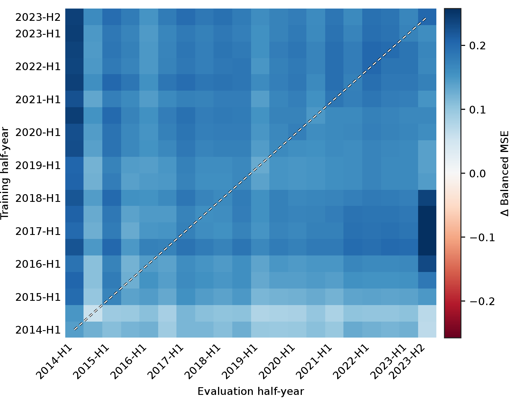

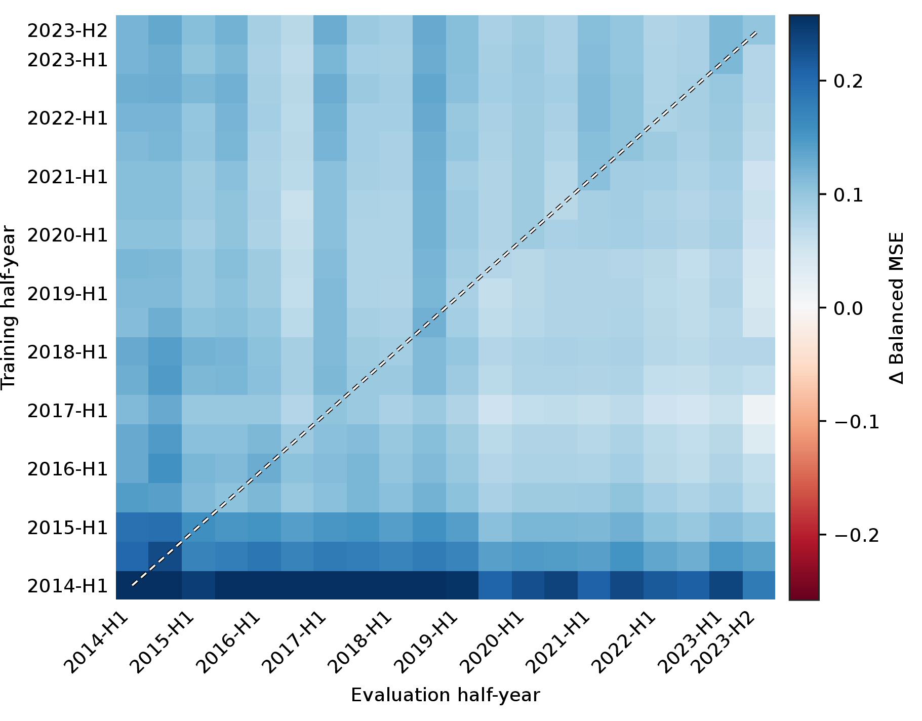

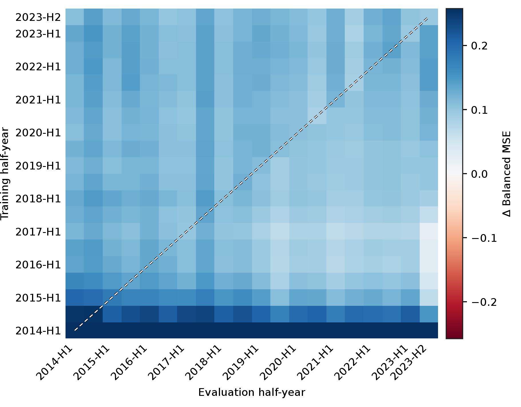

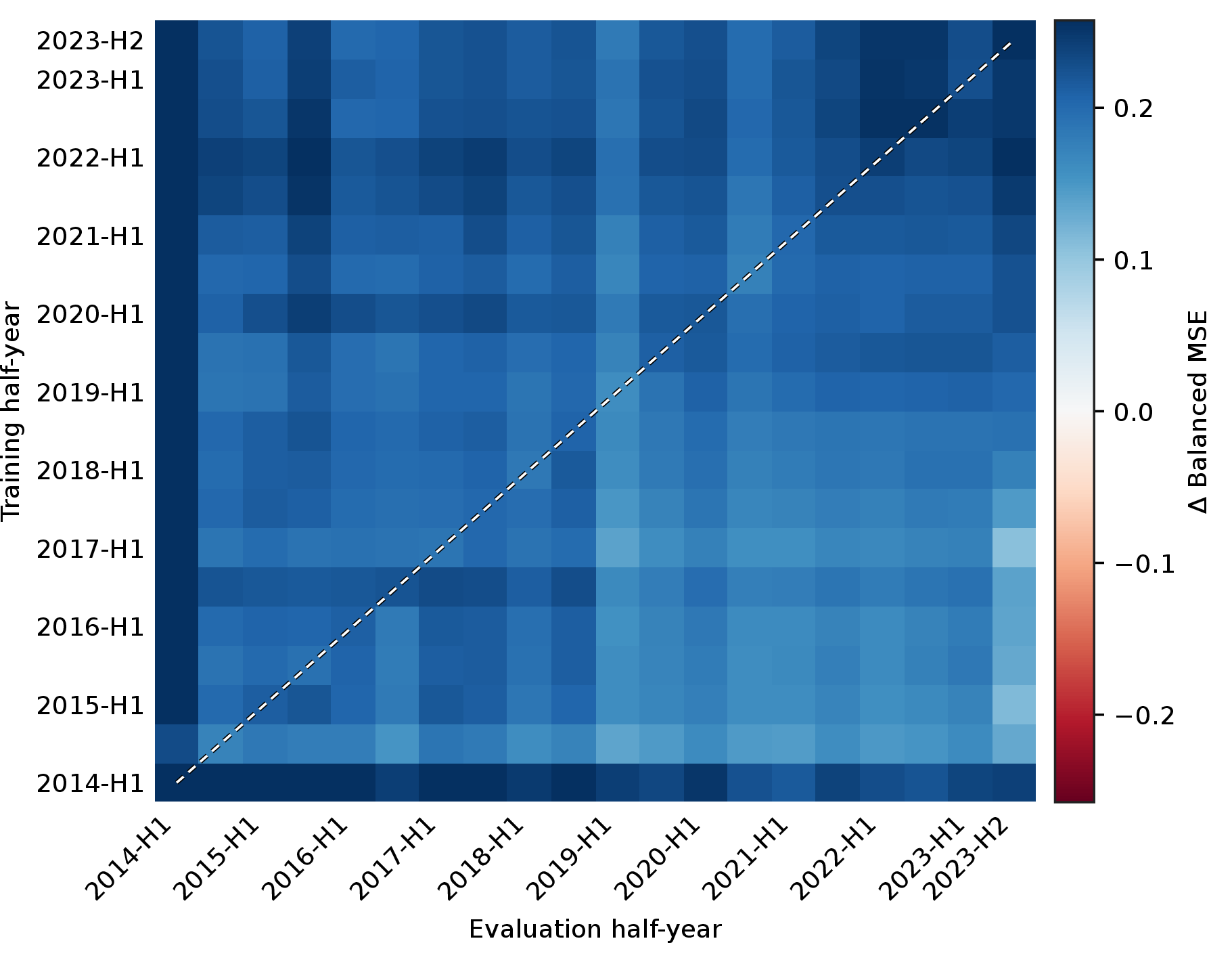

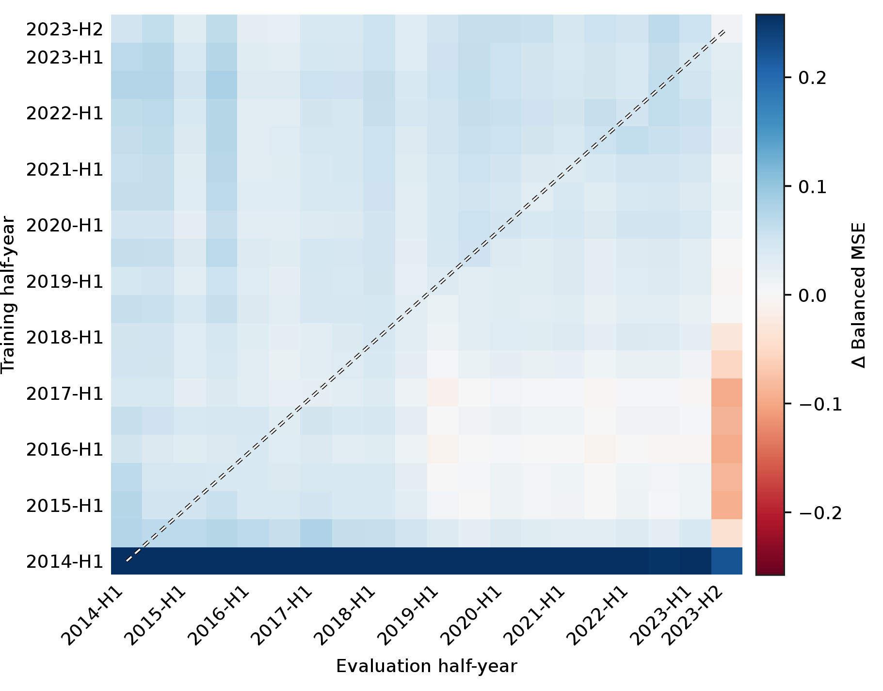

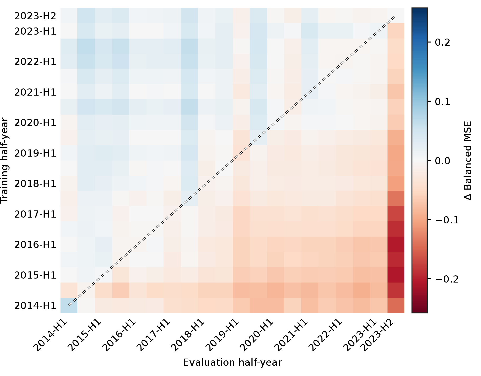
Figure 26: Frozen models: Balanced MSE drift matrix \(M^{(m)}\) and deviation from the cohort mean \(\Delta^{(m)} = M^{(m)} - \bar{M}\) for each model, shown on a sequential and a zero-centred diverging scale, respectively.. b — BERT, d — DistilBERT, f — ELECTRA, h — MPNet, j — ModernBERT, l — RoBERTa, n — DeBERTa-v3
10.7 Forgetting and Rankings↩︎
To see how quickly each model forgets, we summarize its drift matrix as a forgetting curve. The curve plots the Balanced MSE against the lag \(\ell = j - i\), the number of slices between the training cutoff \(i\) and the evaluation slice \(j\). At each lag we average over all training cutoffs, \[F(\ell) = \operatorname{mean}_{i} M_{i,\,i+\ell}.\] The result is the Balanced MSE at a fixed temporal distance, independent of which period a model was trained on. This separates the effect of temporal distance from the difficulty of any single slice.
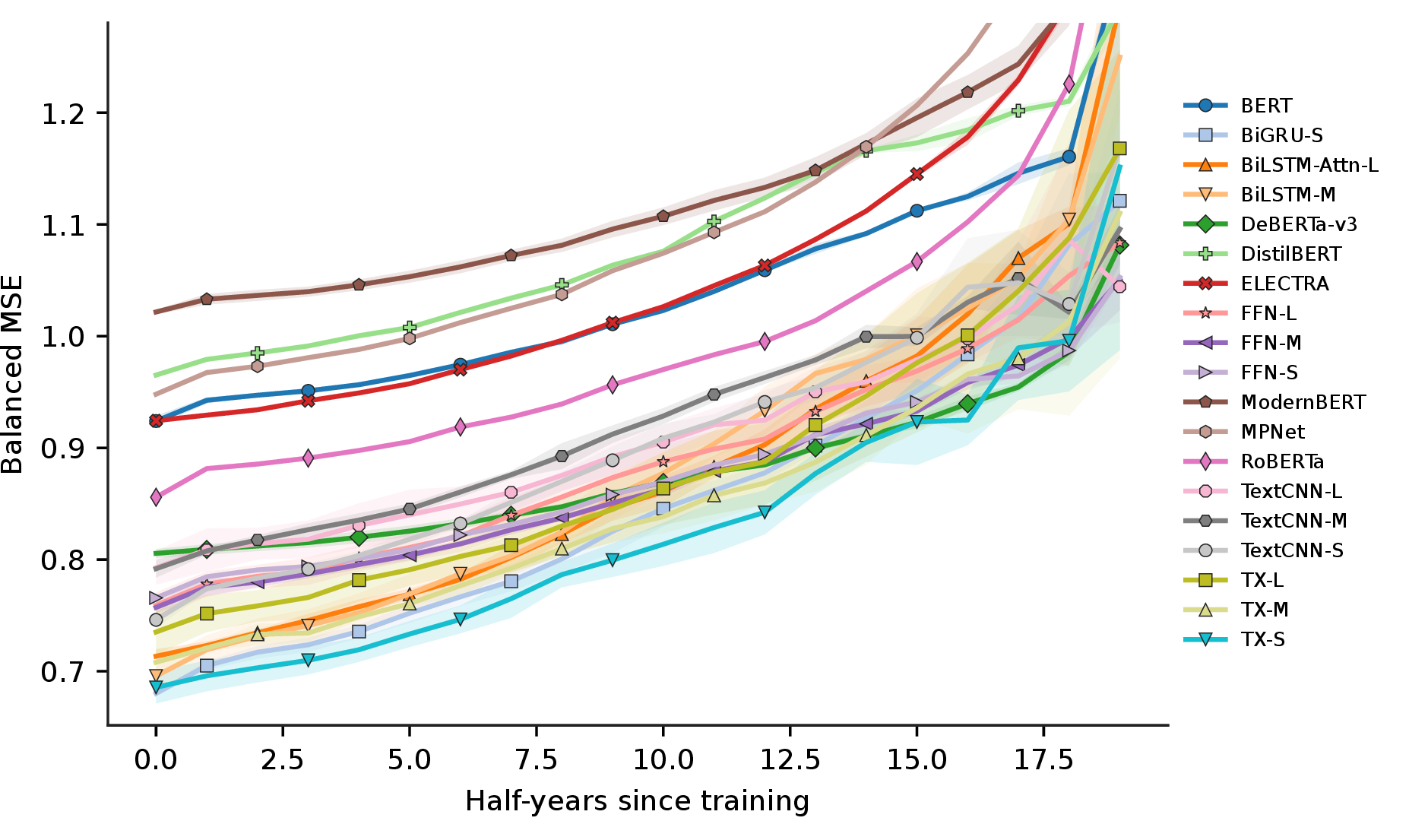
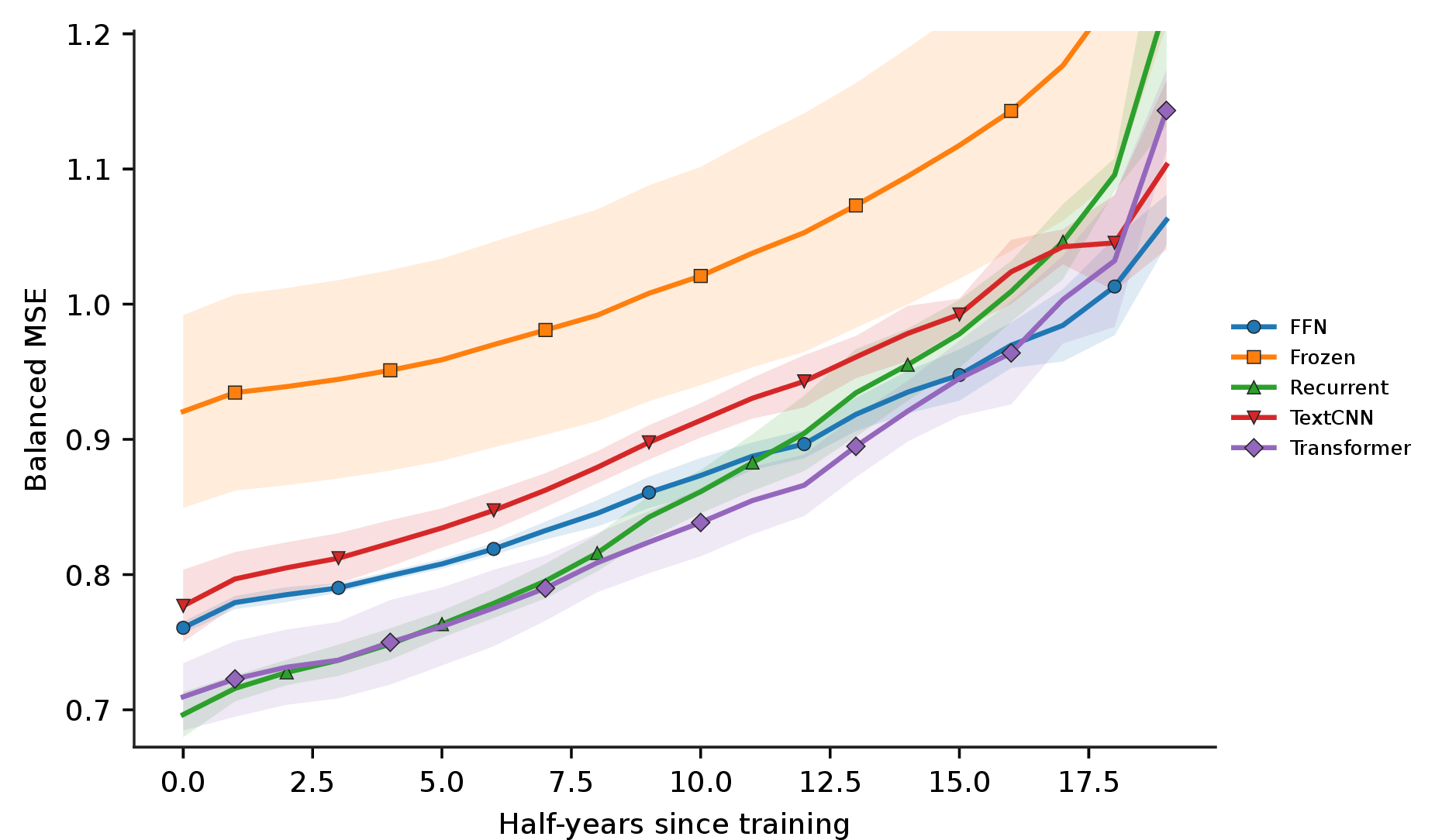
Figure 27: Forgetting curves: each model (left) and averaged within each family (right).. a — Per model, b — Per model family


Figure 28: Models ranked by mean future performance and by temporal decay.. a — By future performance, b — By decay
10.8 Result Tables↩︎

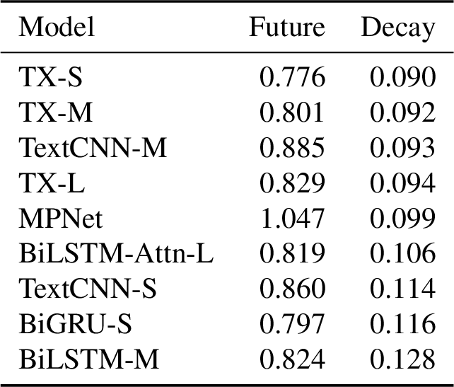
Figure 29:  .
.
Figure 30: 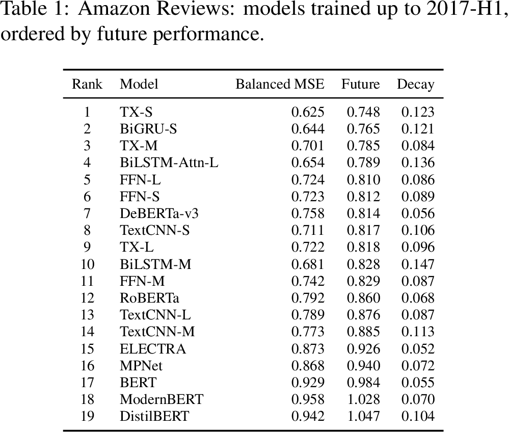 .
.
Figure 31:  .
.
Figure 32: 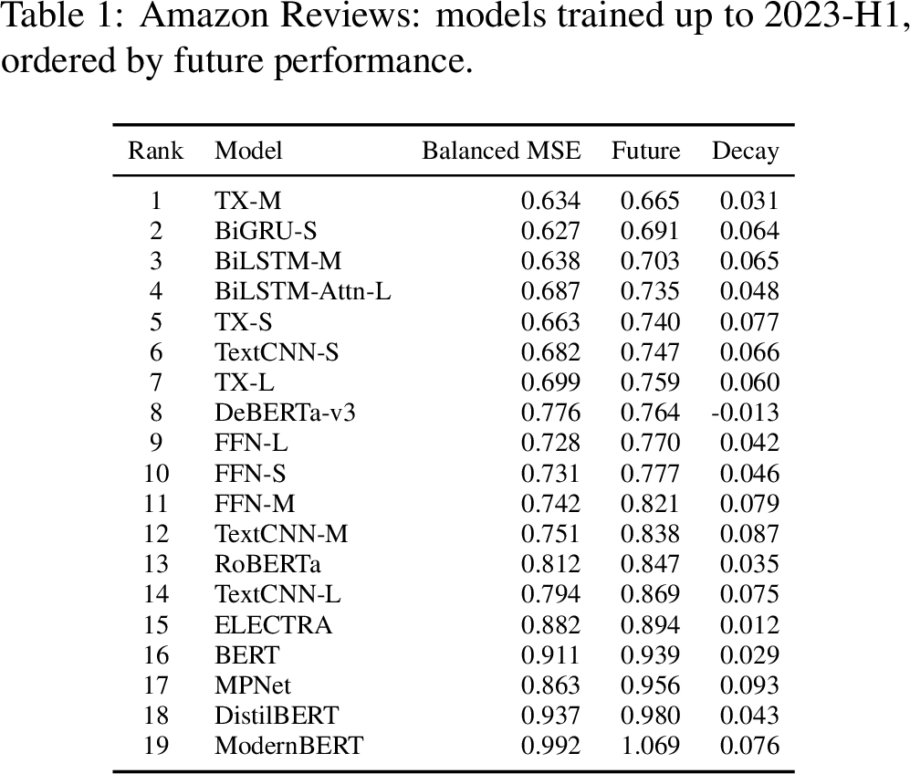 .
.
| 2014-H1 | 2017-H1 | 2020-H1 | 2023-H1 | |||||
| Family | Future | Decay | Future | Decay | Future | Decay | Future | Decay |
| FFN | 0.993 | 0.117 | 0.817 | 0.087 | 0.802 | 0.073 | 0.789 | 0.056 |
| Frozen | 1.351 | 0.131 | 0.943 | 0.068 | 0.934 | 0.073 | 0.921 | 0.039 |
| Recurrent | 1.101 | 0.242 | 0.794 | 0.134 | 0.723 | 0.094 | 0.710 | 0.059 |
| TextCNN | 1.002 | 0.227 | 0.859 | 0.102 | 0.811 | 0.090 | 0.818 | 0.076 |
| Transformer | 0.967 | 0.173 | 0.784 | 0.101 | 0.748 | 0.080 | 0.721 | 0.056 |
11 arXiv – Drift Matrices↩︎
The cohort-mean and per-model deviation matrices shown here, and the in-distribution, future, and decay quantities tabulated below, are defined in Section 4.5. The label space comprises the leaf categories
cs.LG, hep-ph, cs.CV, cs.AI, hep-th, quant-ph, and gr-qc.
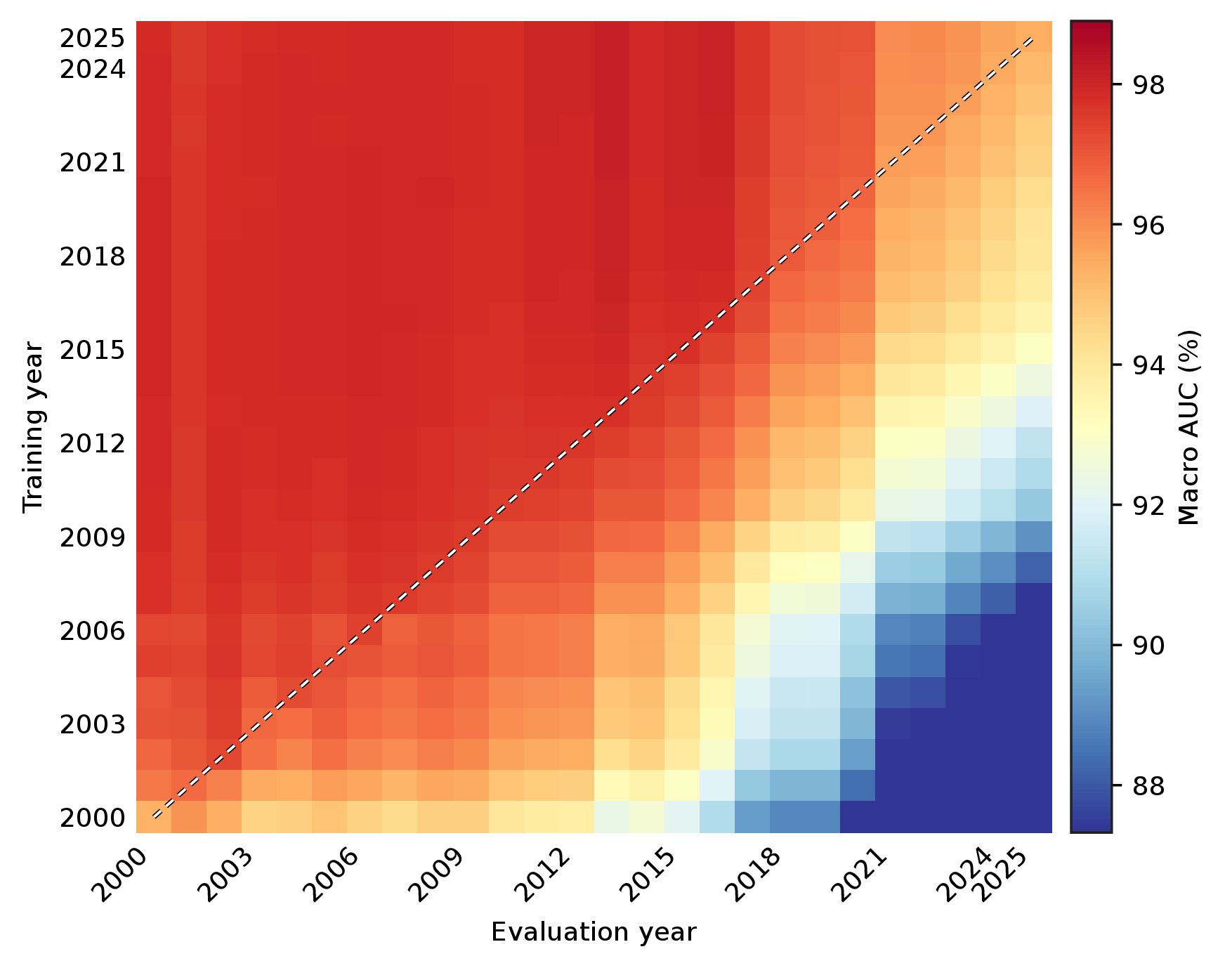
11.1 Model Roster↩︎
Figure 34: 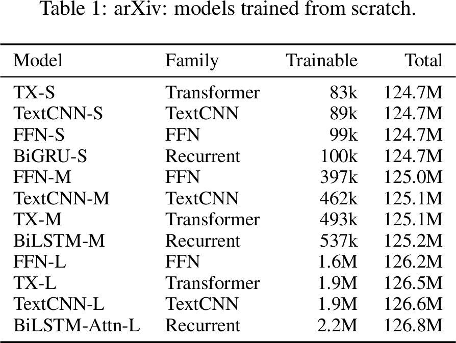 .
.
Figure 35: 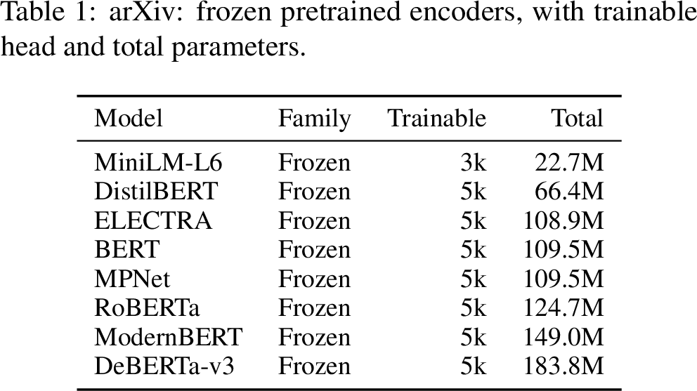 .
.
11.2 FFN↩︎

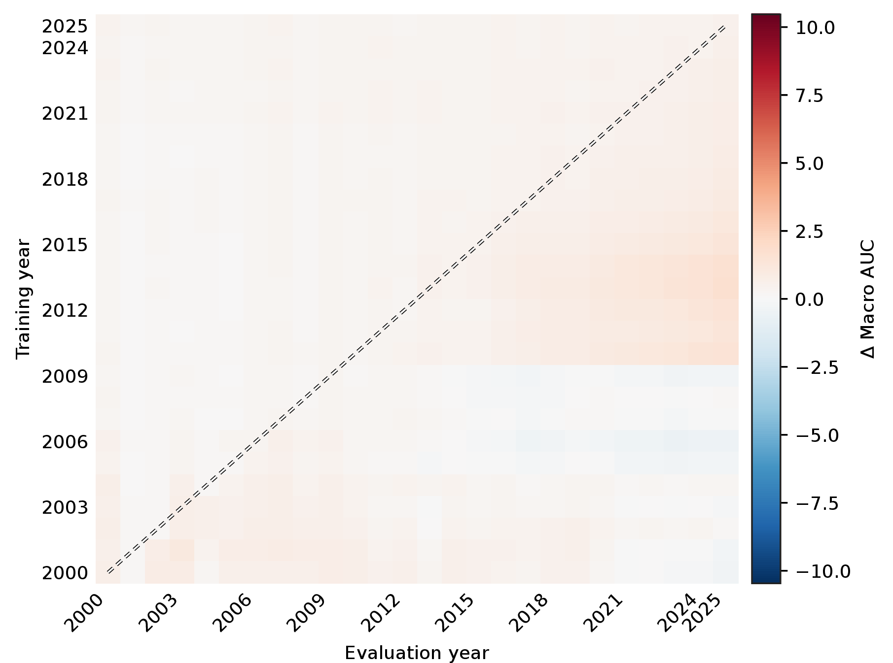

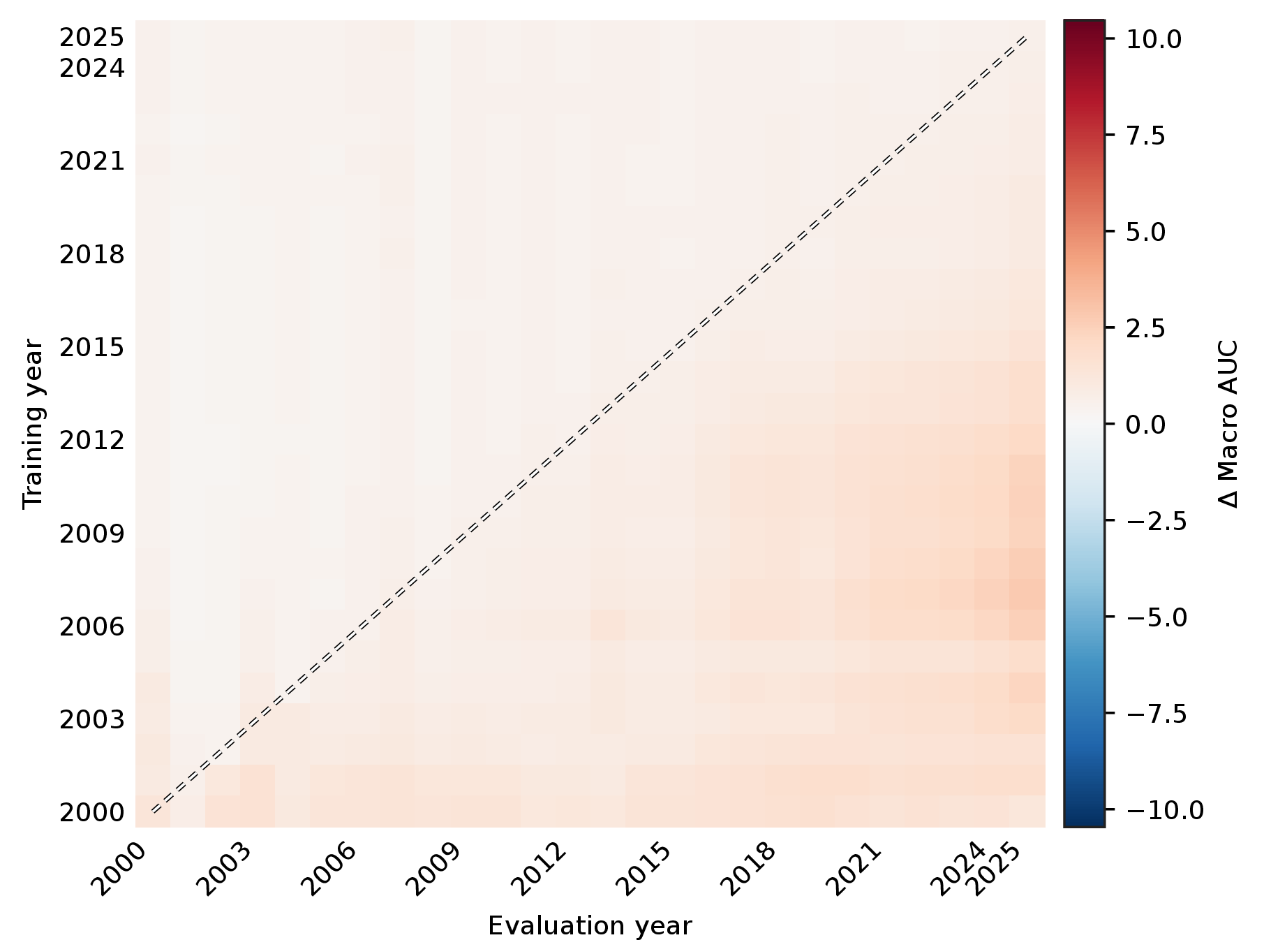

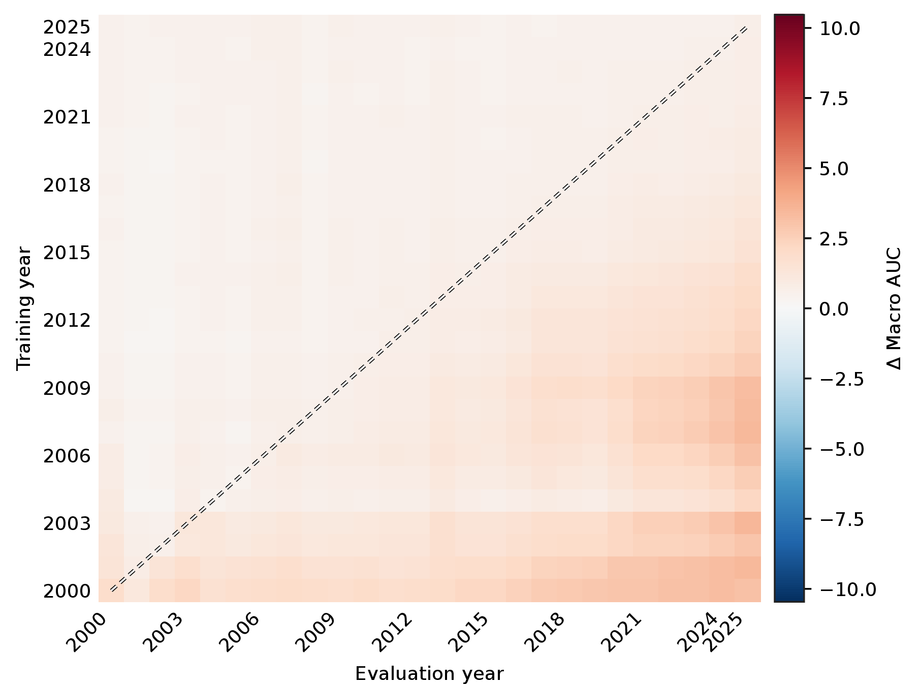
Figure 36: FFN models: Macro AUC drift matrix \(M^{(m)}\) and deviation from the cohort mean \(\Delta^{(m)} = M^{(m)} - \bar{M}\) for each model, shown on a sequential and a zero-centred diverging scale, respectively.. b — FFN-S, d — FFN-M, f — FFN-L
11.3 TextCNN↩︎

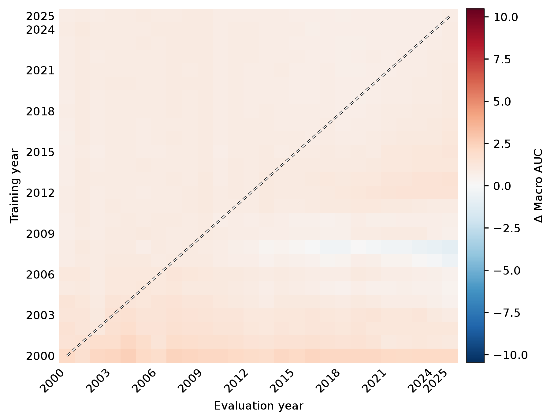

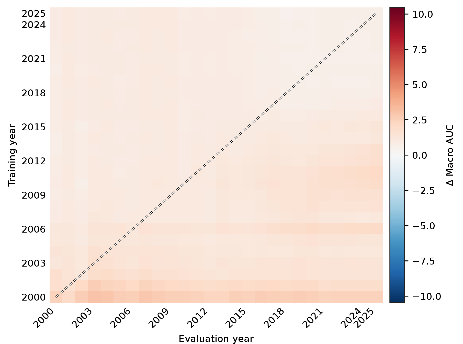

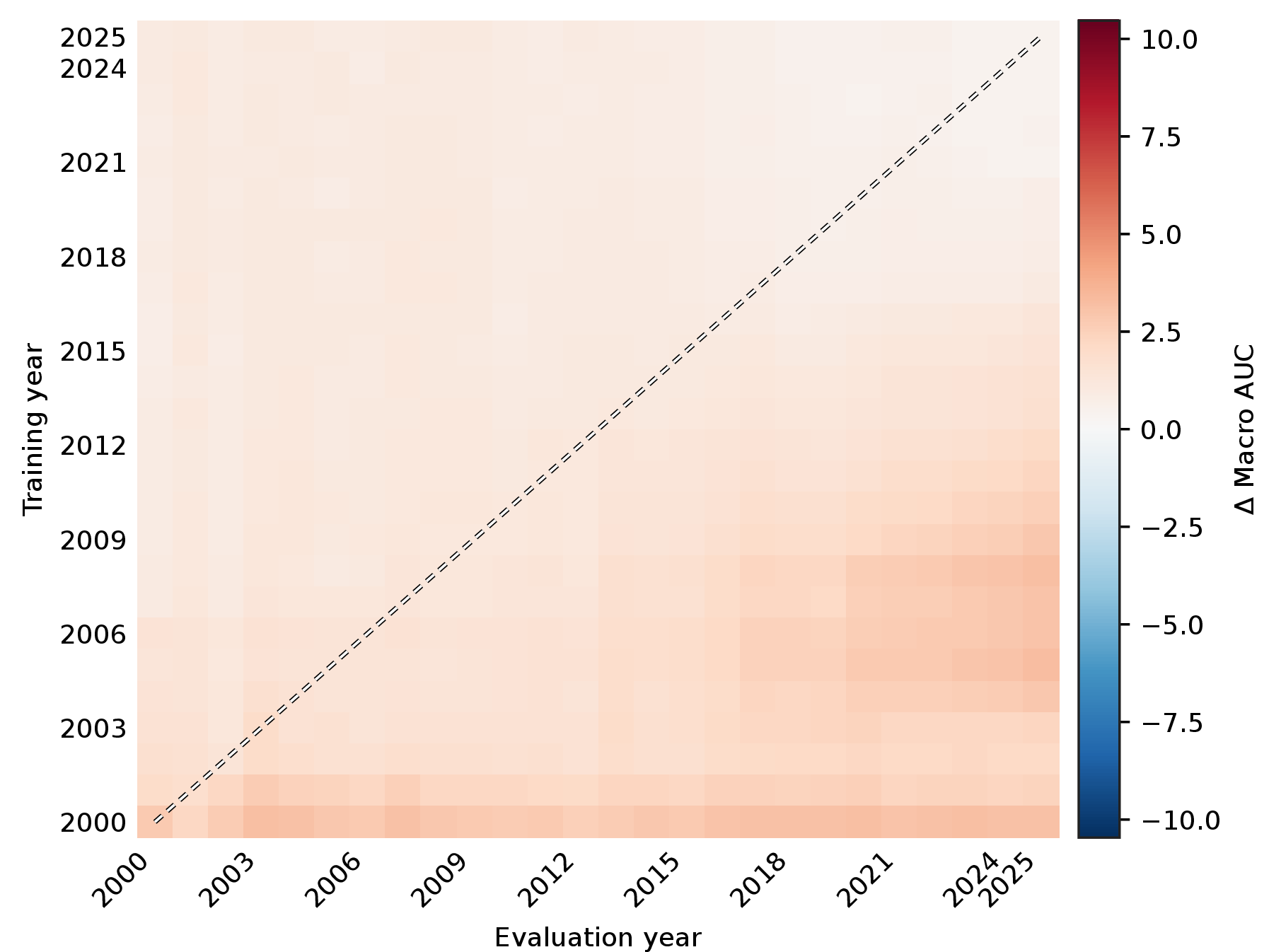
Figure 37: TextCNN models: Macro AUC drift matrix \(M^{(m)}\) and deviation from the cohort mean \(\Delta^{(m)} = M^{(m)} - \bar{M}\) for each model, shown on a sequential and a zero-centred diverging scale, respectively.. b — TextCNN-S, d — TextCNN-M, f — TextCNN-L
11.4 Recurrent↩︎

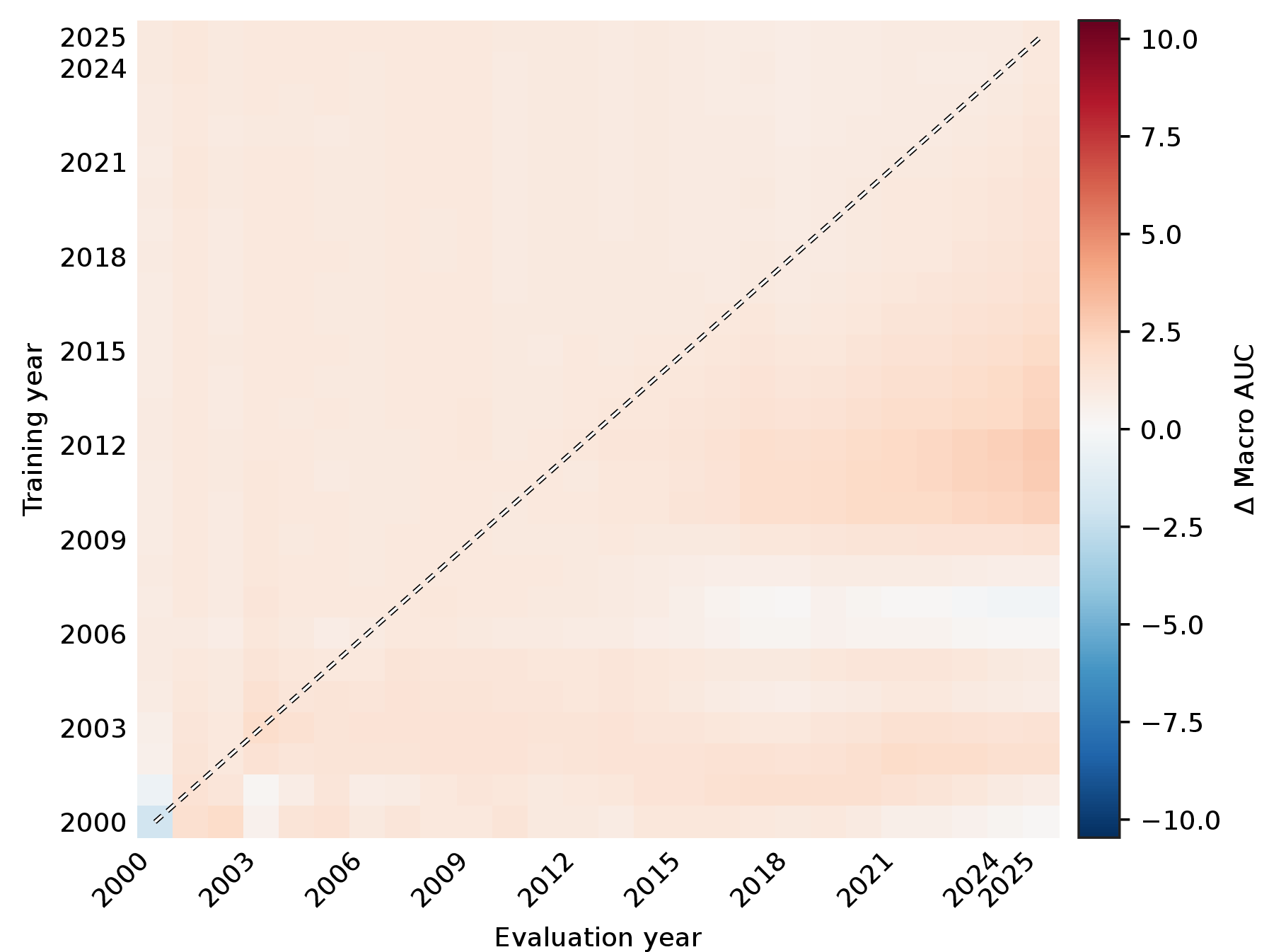

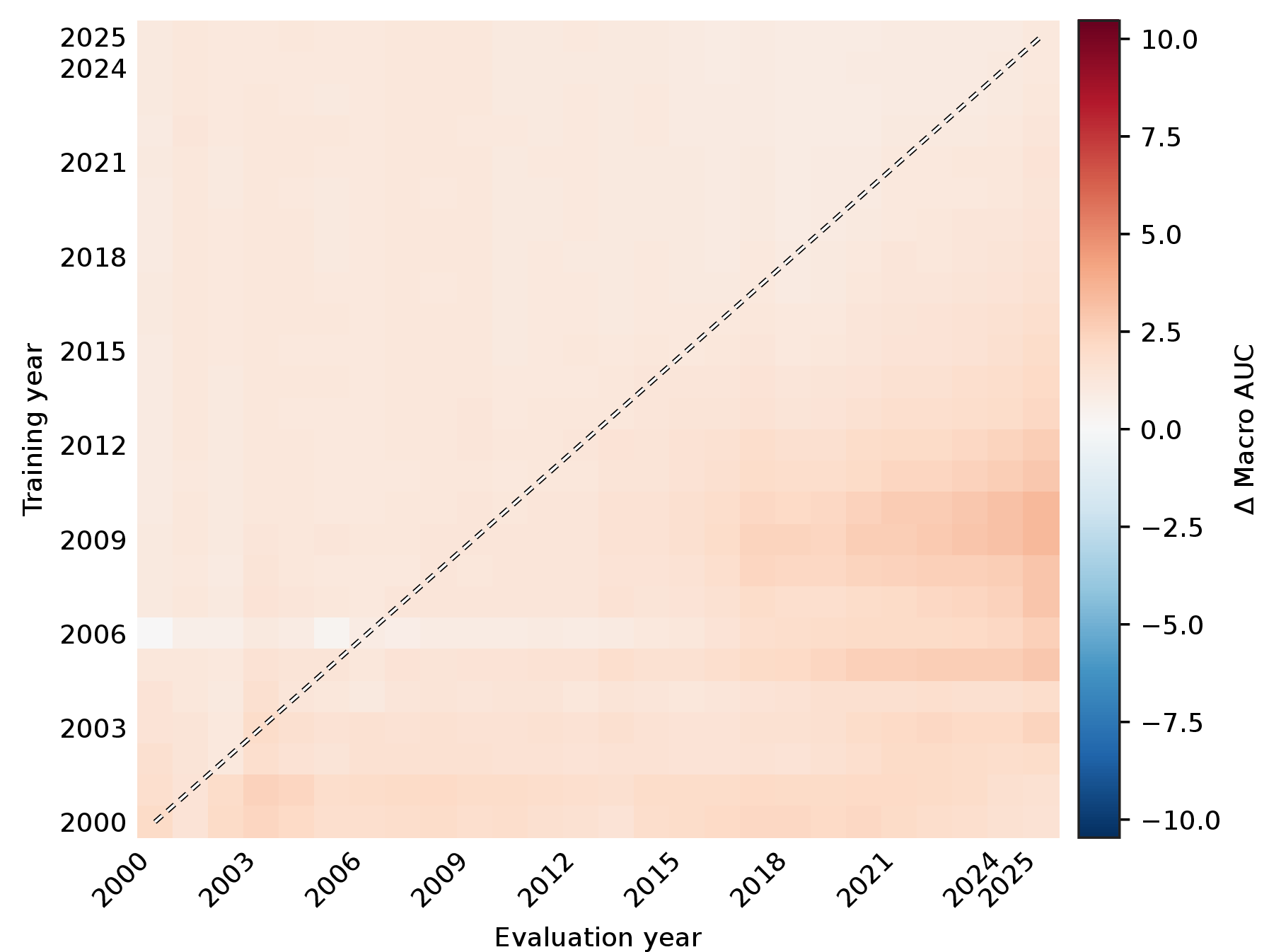

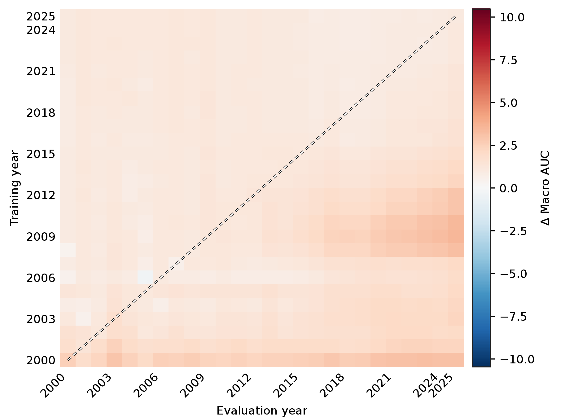
Figure 38: Recurrent models: Macro AUC drift matrix \(M^{(m)}\) and deviation from the cohort mean \(\Delta^{(m)} = M^{(m)} - \bar{M}\) for each model, shown on a sequential and a zero-centred diverging scale, respectively.. b — BiGRU-S, d — BiLSTM-M, f — BiLSTM-Attn-L
11.5 Transformer↩︎

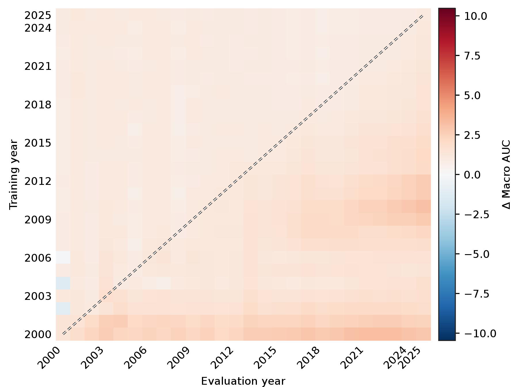

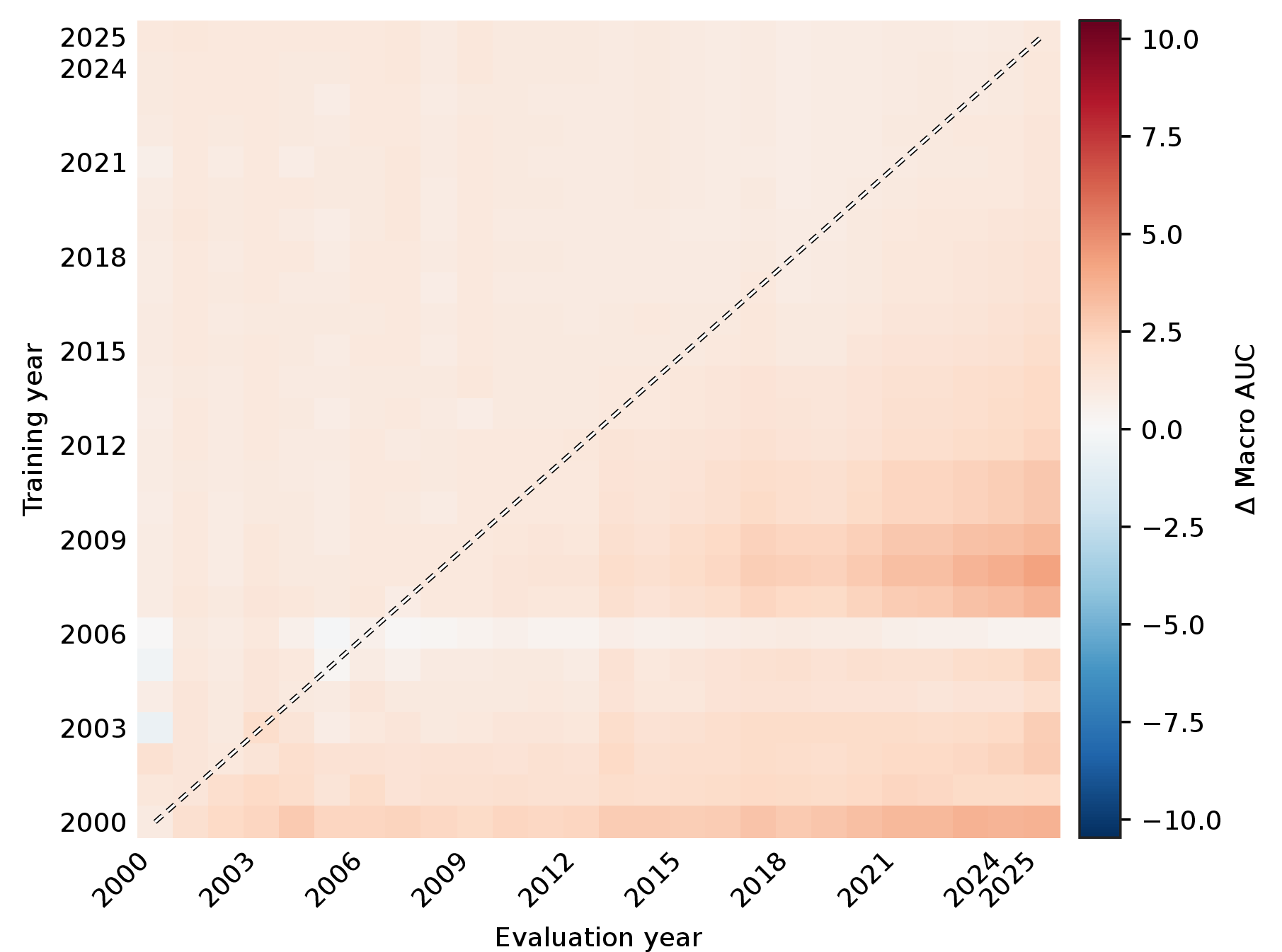

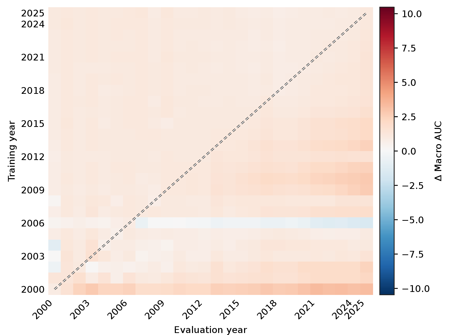
Figure 39: Transformer models: Macro AUC drift matrix \(M^{(m)}\) and deviation from the cohort mean \(\Delta^{(m)} = M^{(m)} - \bar{M}\) for each model, shown on a sequential and a zero-centred diverging scale, respectively.. b — TX-S, d — TX-M, f — TX-L
11.6 Frozen↩︎

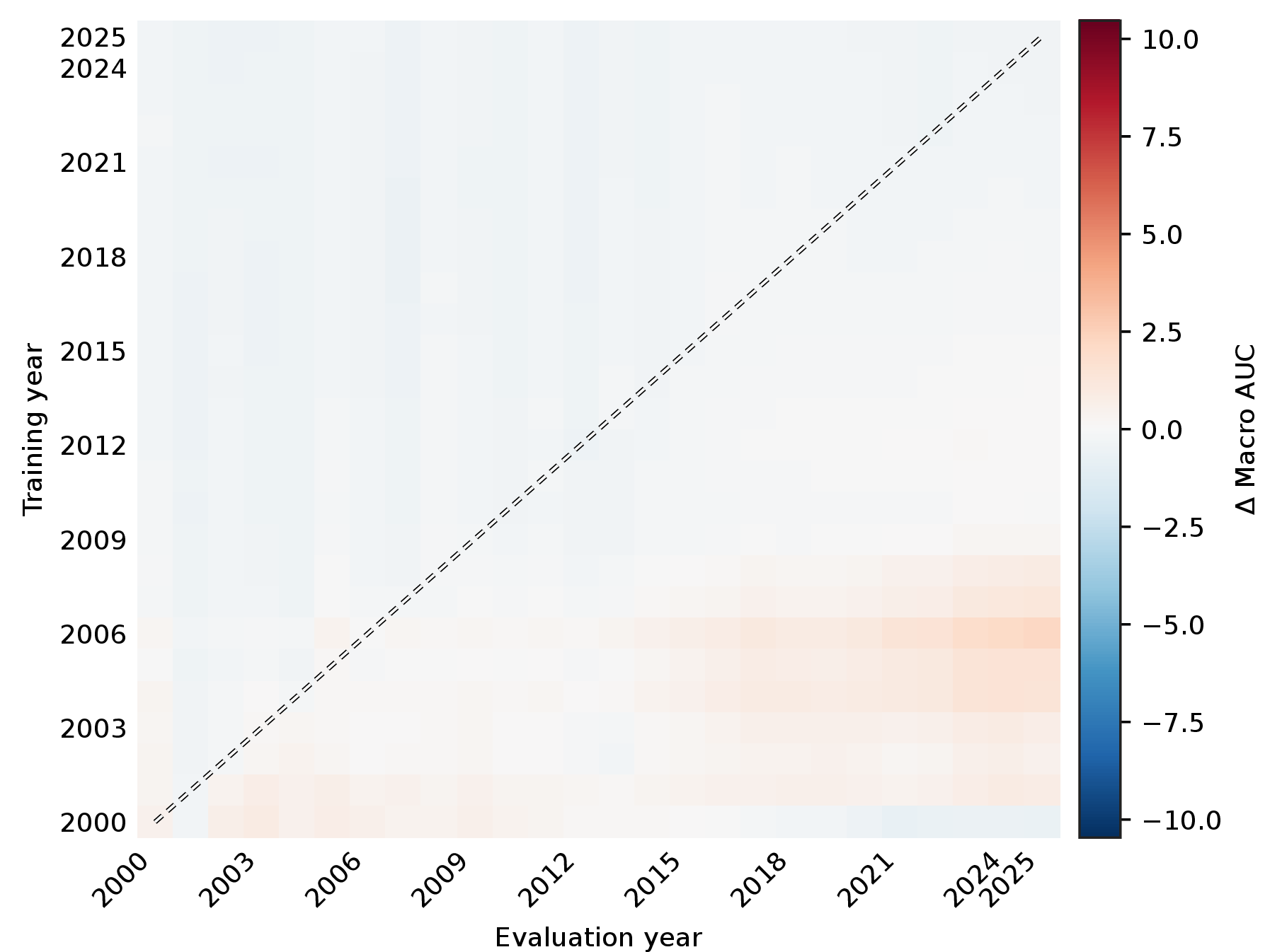

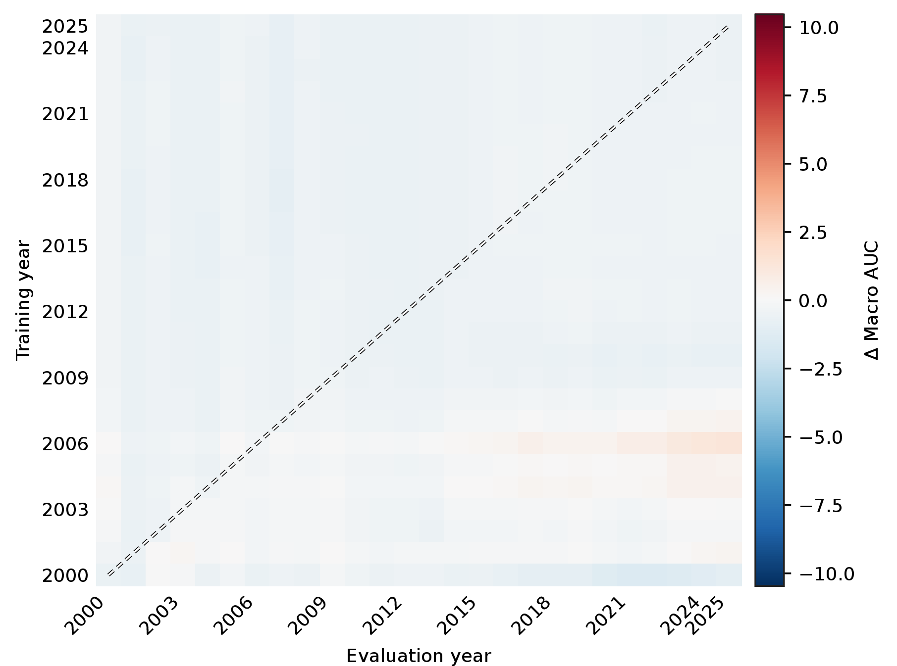

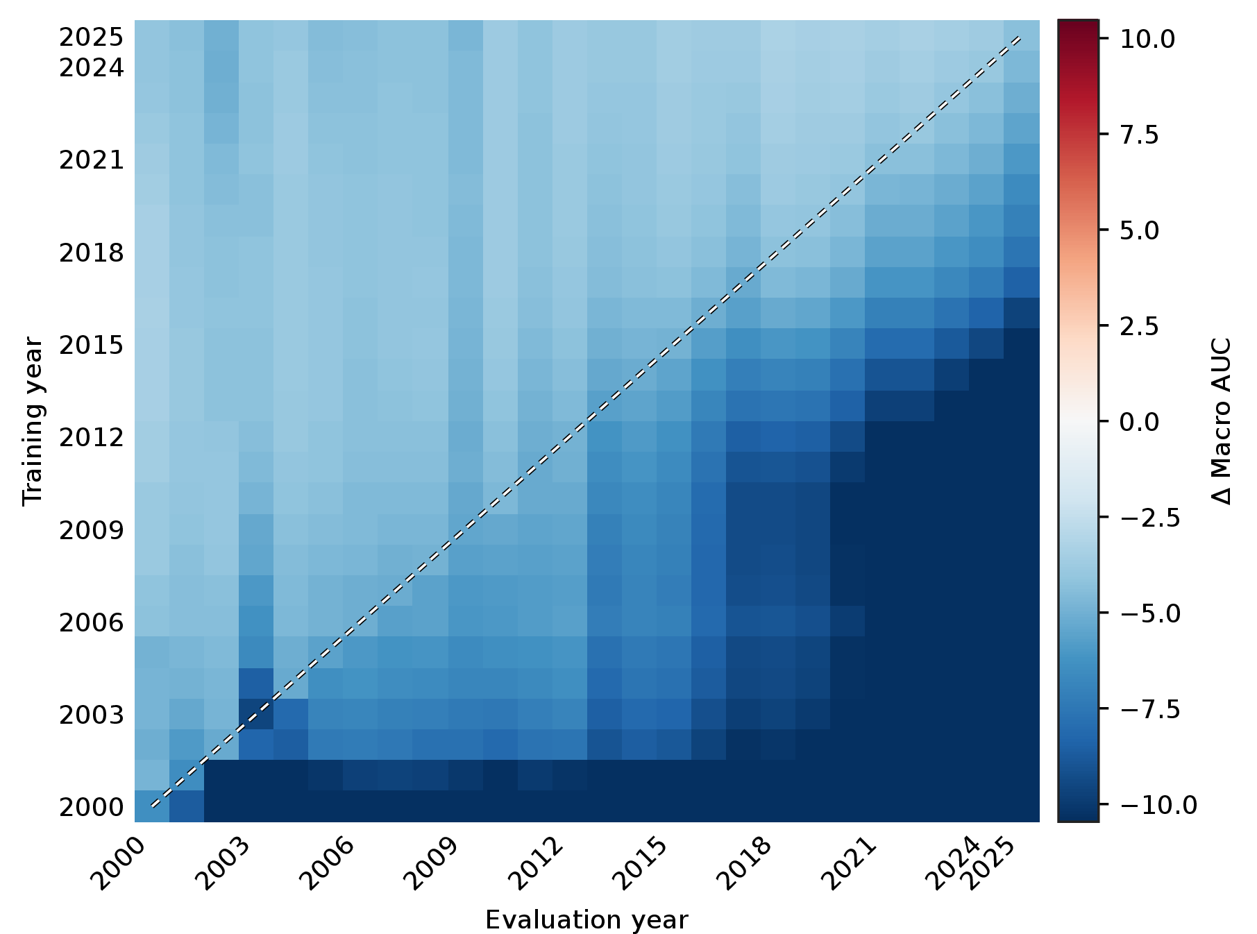

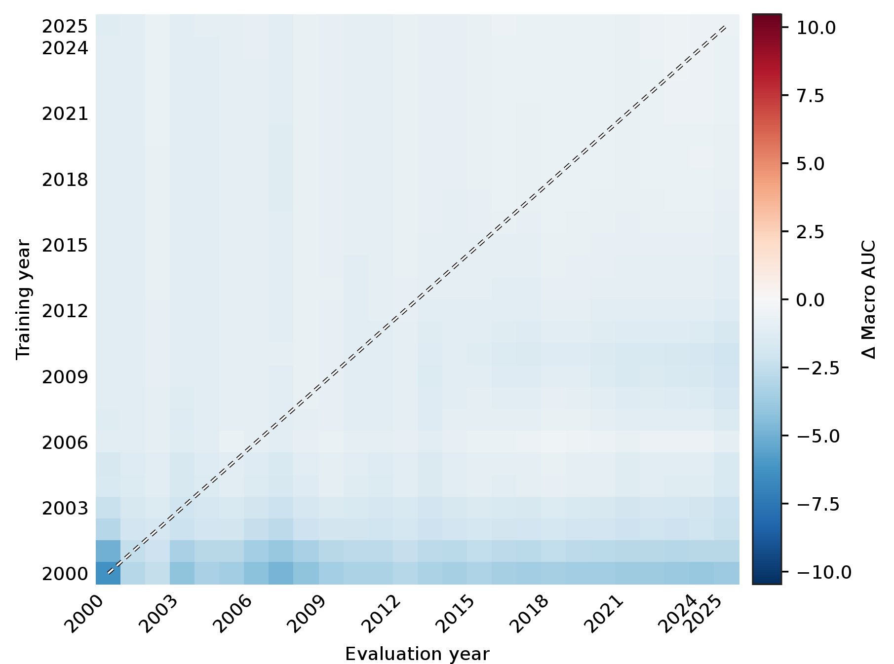


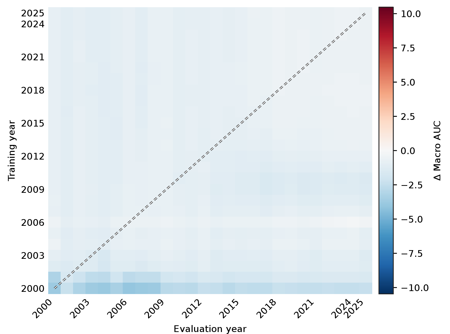

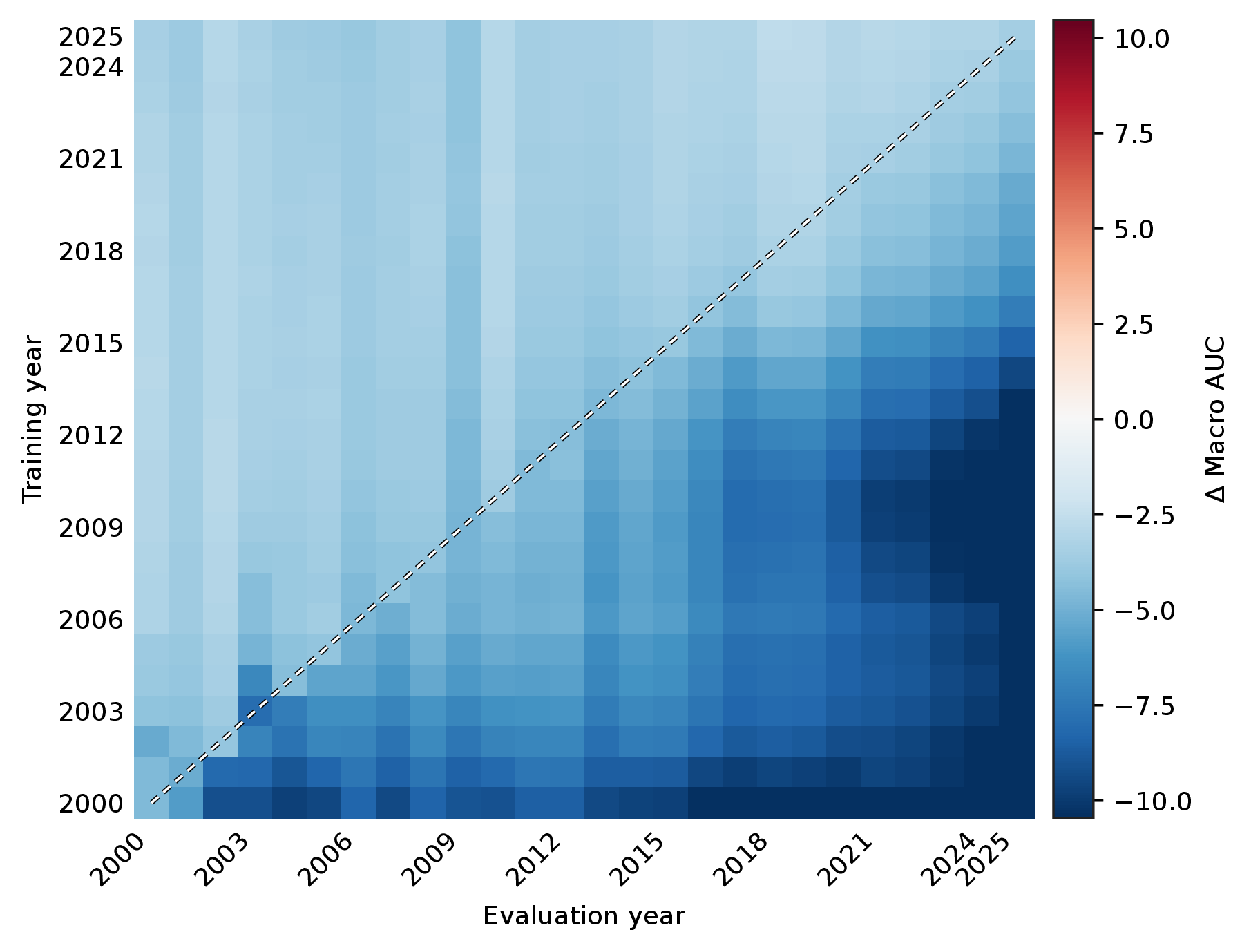

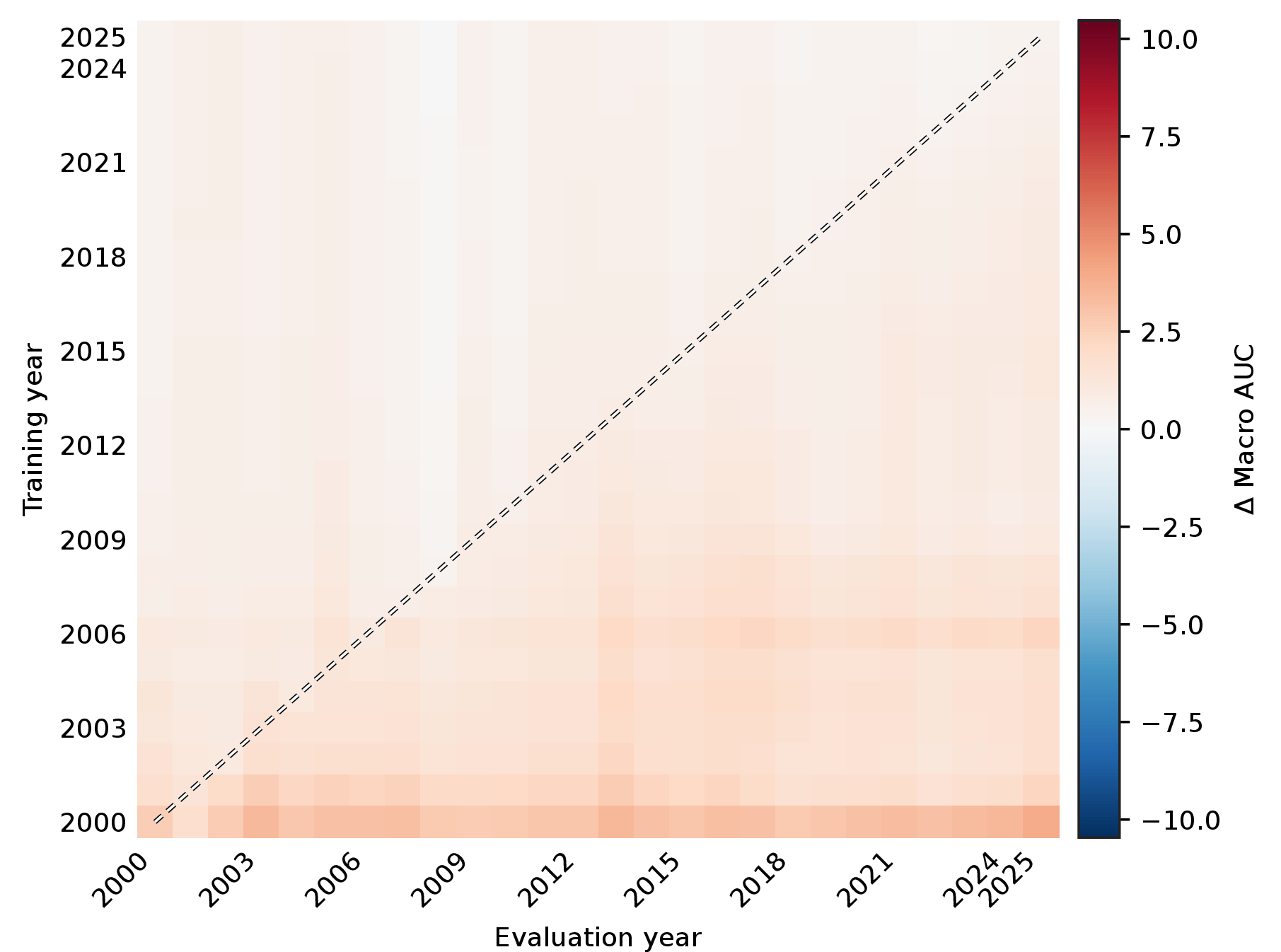
Figure 40: Frozen models: Macro AUC drift matrix \(M^{(m)}\) and deviation from the cohort mean \(\Delta^{(m)} = M^{(m)} - \bar{M}\) for each model, shown on a sequential and a zero-centred diverging scale, respectively.. b — BERT, d — DistilBERT, f — ELECTRA, h — MPNet, j — ModernBERT, l — RoBERTa, n — DeBERTa-v3, p — MiniLM-L6
11.7 Forgetting and Rankings↩︎
To see how quickly each model forgets, we summarize its drift matrix as a forgetting curve. The curve plots the Macro AUC against the lag \(\ell = j - i\), the number of slices between the training cutoff \(i\) and the evaluation slice \(j\). At each lag we average over all training cutoffs, \[F(\ell) = \operatorname{mean}_{i} M_{i,\,i+\ell}.\] The result is the Macro AUC at a fixed temporal distance, independent of which period a model was trained on. This separates the effect of temporal distance from the difficulty of any single slice.
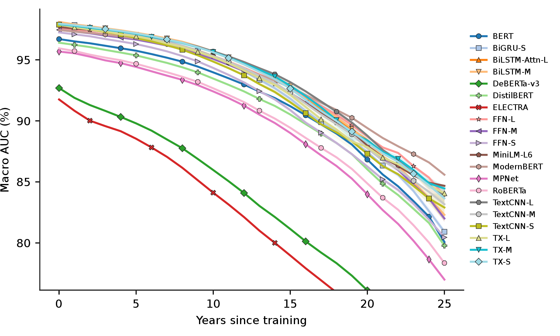
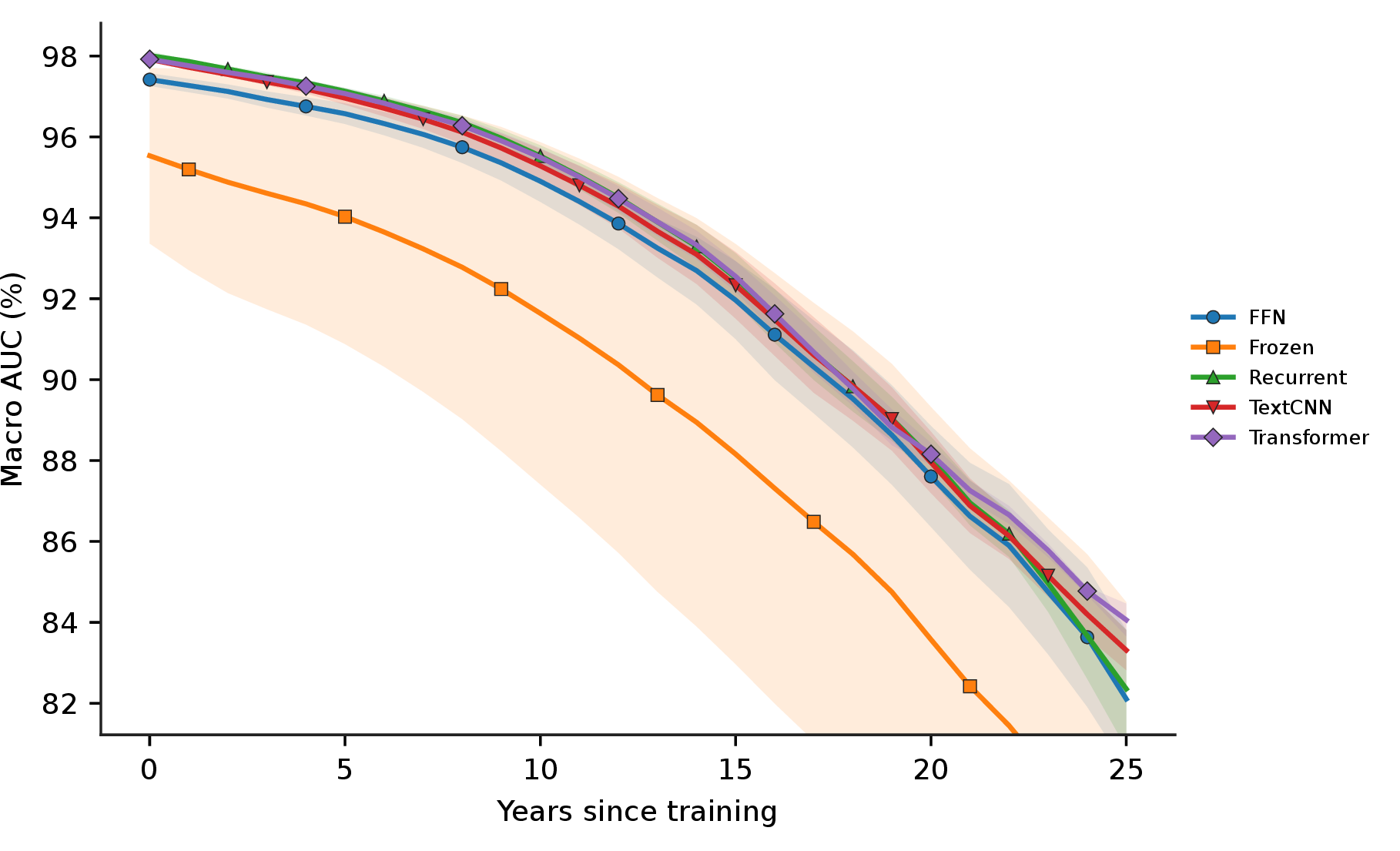
Figure 41: Forgetting curves: each model (left) and averaged within each family (right).. a — Per model, b — Per model family


Figure 42: Models ranked by mean future performance and by temporal decay.. a — By future performance, b — By decay
11.8 Result Tables↩︎
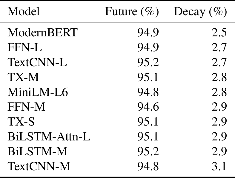
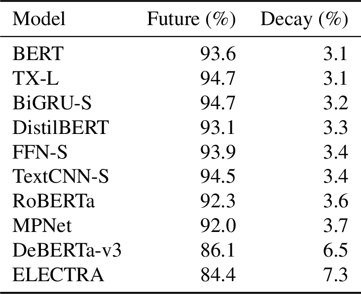
Figure 43: 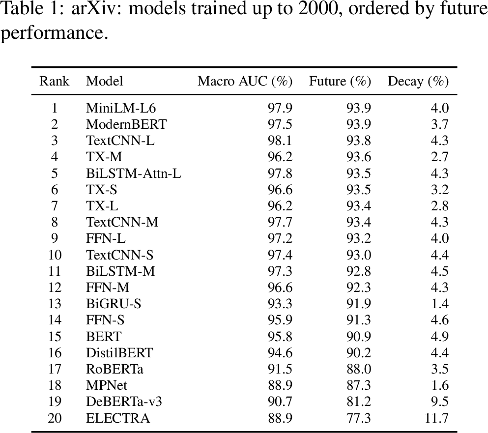 .
.
Figure 44:  .
.
Figure 45: 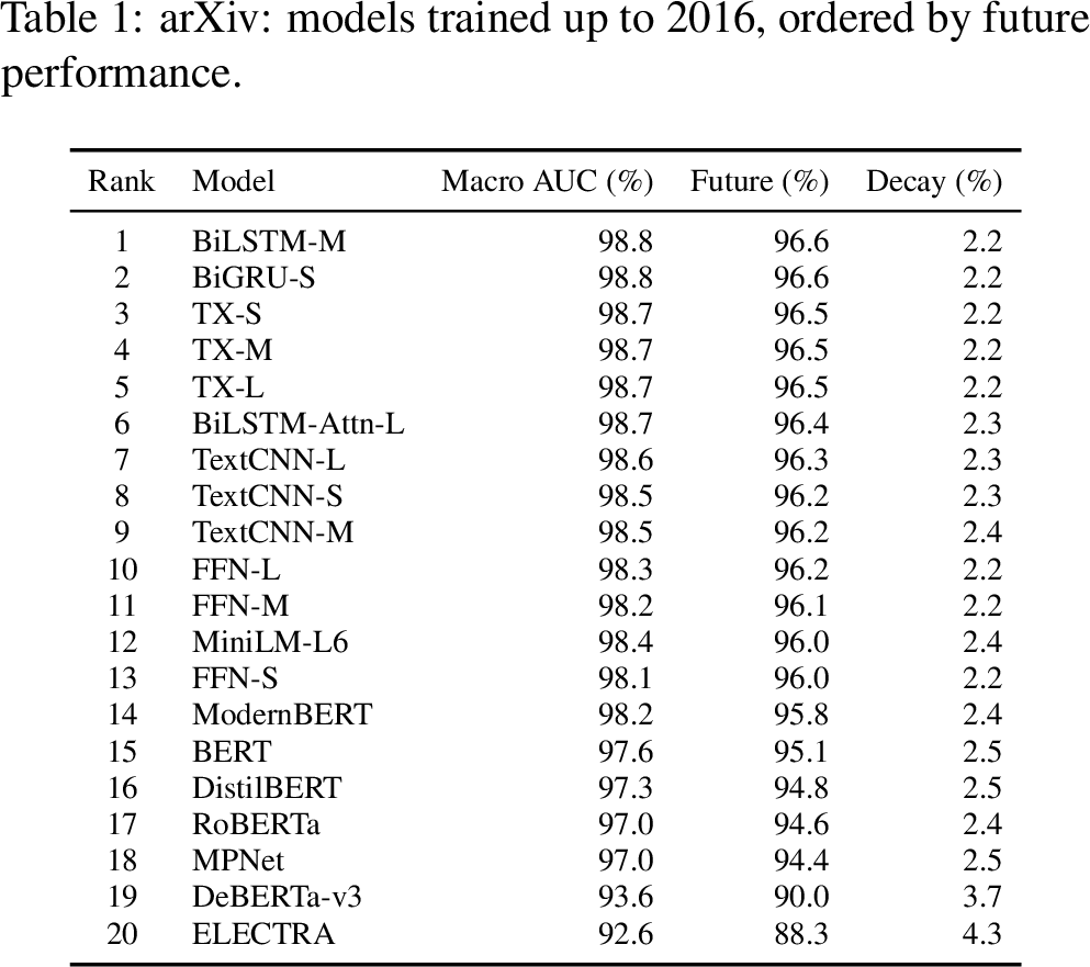 .
.
Figure 46: 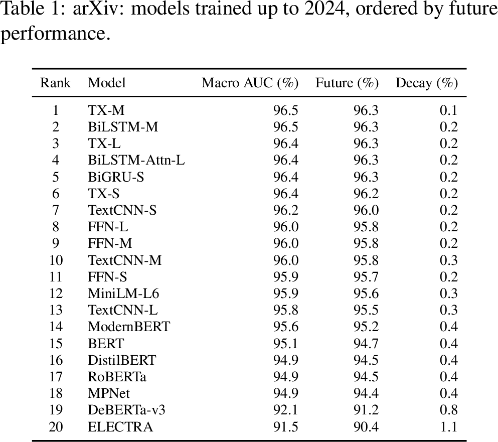 .
.
| 2000 | 2008 | 2016 | 2024 | |||||
| Family | Future | Decay | Future | Decay | Future | Decay | Future | Decay |
| FFN | 92.2 | 4.3 | 94.6 | 3.3 | 96.1 | 2.2 | 95.8 | 0.2 |
| Frozen | 87.8 | 5.4 | 91.6 | 4.6 | 93.6 | 2.8 | 93.8 | 0.5 |
| Recurrent | 92.7 | 3.4 | 95.2 | 3.4 | 96.5 | 2.2 | 96.3 | 0.2 |
| TextCNN | 93.4 | 4.3 | 94.7 | 3.9 | 96.2 | 2.3 | 95.8 | 0.3 |
| Transformer | 93.5 | 2.9 | 95.4 | 3.0 | 96.5 | 2.2 | 96.3 | 0.2 |