Level-Crossing Density as a Mesh-Free High-Frequency
Auxiliary Loss for Implicit Neural Representations
July 07, 2026
Abstract
Coordinate-MLP implicit neural representations (INRs) exhibit spectral bias: they fit low-frequency structure quickly and high-frequency detail slowly or not at all. Existing remedies act in the frequency domain (e.g., the Focal Frequency Loss), on activations and encodings (SIREN, Fourier features, FINER), or through coarse-to-fine curricula—and the loss-based remedies presuppose a regular sampling grid on which a discrete Fourier transform is available. We revisit a classical object from random-field theory, the Rice level-crossing density, and turn it into a differentiable training objective. By the co-area formula, the density of level crossings of a field is a direct functional of its gradient magnitude concentrated on level sets, and for stationary processes it is monotone in the ratio of spectral moments \(\sqrt{\lambda_2/\lambda_0}\)—i.e., it is a spatial-domain, closed-form proxy for high-frequency content. We construct a smoothed Monte-Carlo estimator of the crossing density that is evaluated pointwise at arbitrary sample locations, requires no grid, no FFT, and no mesh, and match it to the empirical crossing density of the supervision signal across a set of levels. We validate the estimator against exact crossing counts and the Rice formula, then evaluate the loss under strict information parity against the Focal Frequency Loss, normalized Sobolev supervision, and MSE-only training, on regular grids and on scattered non-uniform samples, and we report the outcome without embellishment. Where supervision is scarce and irregular, every auxiliary spectral loss is transformative (\(+2.3\)–\(3.0\) dB over MSE-only on PE-MLP, \(+1.4\)–\(1.8\) dB on SIREN); on an edge-dominated natural image the crossing-density loss matches the alternatives—within \(0.2\)–\(0.5\) dB of FFL on PSNR, matching or exceeding it on SSIM—without beating them, while on a statistically homogeneous texture, the regime closest to the stationary fields of the Rice theory, it overtakes FFL by \(0.6\) dB. Its further distinctions are structural: it is the only loss requiring neither a sampling grid nor trustworthy pointwise gradient targets, and an oracle-gradient diagnostic shows it is uniquely insensitive to gradient-target quality. On dense regular grids, where auxiliary drives are unnecessary, finite-difference gradient targets actively hurt—a caution that applies equally to Sobolev training. We release code, raw results, and all experiment scripts.
1 Introduction↩︎
Implicit neural representations (INRs) parameterize a signal as a neural network \(f_\theta:\mathbb{R}^d\to\mathbb{R}^m\) mapping coordinates to values, and have become a standard representation for images, signed distance fields, and radiance fields [1]–[4]. Their best-known failure mode is spectral bias [5], [6]: trained with a plain reconstruction loss, coordinate MLPs learn low frequencies first and high frequencies slowly, blurring fine detail. The community’s responses fall into three families: (i) architectural fixes—Fourier feature encodings [7], periodic activations [1], their variable-periodic [8], wavelet [9], and Gaussian [10] relatives, multiplicative filter networks [11], band-limited architectures [12], and hash grids [13]; (ii) loss-based fixes—frequency-domain objectives such as the Focal Frequency Loss (FFL) [14] and gradient-domain (Sobolev) supervision [15], [16]; and (iii) curricula that schedule frequency content coarse-to-fine [17], [18].
The loss-based family has a structural blind spot. A discrete Fourier transform is defined on a regular grid. When supervision arrives as scattered samples—point clouds for neural SDFs, non-uniformly sampled sensor data, adaptively sampled renderings—a frequency-domain loss must first resample the scattered data onto a grid, and the interpolation step smears exactly the high-frequency content the loss is meant to supervise. Gradient-matching losses are pointwise and thus mesh-free, but they supervise the gradient at each point, so their targets inherit, pointwise and at full strength, whatever noise the gradient-estimation step introduces.
This paper proposes a third kind of spatial-domain objective, borrowed from random-field theory. The Rice formula [19], [20] states that for a stationary Gaussian process the expected number of crossings of level \(u\) per unit length is \[\mu(u) \;=\; \frac{1}{\pi}\sqrt{\frac{\lambda_2}{\lambda_0}}\; e^{-u^2/(2\lambda_0)}, \qquad \lambda_k = \int \omega^k \, dS(\omega), \label{eq:rice}\tag{1}\] where \(S\) is the spectral measure. The crossing rate is monotone in \(\sqrt{\lambda_2/\lambda_0}\), the RMS angular frequency: how often a field crosses a level is a direct, closed-form functional of how much high-frequency energy it carries. This link between zero-crossing rates and spectral content is classical in signal processing [21], [22]; our contribution is not the link itself but its instantiation as a differentiable training objective for INRs, and an empirical study of where such an objective helps.
Concretely, we estimate the crossing density of the INR’s output field with a smoothed Monte-Carlo form of the Kac–Rice integrand, \[\hat{c}_\varepsilon(u) \;=\; \frac{1}{N}\sum_{i=1}^N \delta_\varepsilon\!\bigl(f_\theta(x_i)-u\bigr)\, \bigl\lVert \nabla_x f_\theta(x_i)\bigr\rVert, \label{eq:estimator}\tag{2}\] where the \(x_i\) are the (arbitrary, possibly scattered) training coordinates, \(\delta_\varepsilon\) is a Gaussian bump, and \(\nabla_x f_\theta\) is exact via automatic differentiation. By the co-area formula, 2 estimates crossings per unit length in 1D, level-set length per unit area in 2D, and level-set area per unit volume in 3D. The auxiliary loss matches \(\hat{c}_\varepsilon(u)\) to the empirical crossing density of the ground truth at a small set of levels. Everything is pointwise: no grid, no FFT, no mesh, no stationarity or Gaussianity assumption.
Because a crossing-density profile is a distributional statistic—an average over the whole batch—it discards phase information: it says how much level-set geometry the field should have, not where. It is therefore an auxiliary drive alongside a reconstruction loss (which anchors locations), not a stand-alone objective, and its distributional character is exactly what we expect to make it robust on scattered domains: pointwise errors in derived gradient targets average out in 2 instead of being enforced point by point.
1.0.0.1 Claims.
We make three claims, each tested in Section 5. (1) The estimator 2 is an accurate, differentiable crossing-density estimator (validated against exact counts and against 1 ). (2) As an auxiliary loss it is a working high-frequency drive: wherever supervision is scarce it recovers most of the gap between MSE-only training and the information ceiling set by the samples, on two different backbones. (3) Against the strongest loss-based alternatives under strict information parity, it achieves PSNR parity on edge-dominated natural-image content (with SSIM matching or exceeding FFL’s and unique robustness to gradient-target quality) and overtakes FFL only on statistically homogeneous texture—the regime the Rice theory actually describes. We consider the disciplined measurement of (3), including its negative component, a contribution: the hypothesis that crossing statistics would broadly beat resampled frequency losses off-grid was plausible, cheap to state, and is here tested and bounded.
1.0.0.2 What we do not claim.
Coarse-to-fine frequency curricula exist [17], [18] and we do not claim one. The crossing-rate–frequency link is textbook [21]; we claim only the differentiable-loss instantiation and its evaluation. On regular grids we expect, and report, rough parity rather than dominance.
2 Related work↩︎
2.0.0.1 Spectral bias and architectural remedies.
Spectral bias was characterized by [5], with [6] extending the analysis to non-uniform input densities—directly relevant to our scattered-sampling setting, since their theory predicts that convergence at a given frequency slows further in sparsely sampled regions. Fourier feature encodings [7] and periodic activations [1] move the representable band up; FINER [8] makes the supported band tunable via variable-periodic activations; WIRE [9], Gaussian activations [10], multiplicative filter networks [11], BACON [12], and hash encodings [13] are alternative routes. All of these change the architecture; our proposal is orthogonal and combines with them (Section 5.4).
2.0.0.2 Loss-based remedies.
The Focal Frequency Loss [14] compares DFT spectra of prediction and target with an adaptive per-frequency weight and is the standard frequency-domain objective; it requires a regular grid. Sobolev training supervises derivatives [15], applied to INRs with finite-difference image derivatives by [16]; it is mesh-free but pointwise. Eikonal-type losses in shape representation [23] likewise constrain \(\lVert\nabla f\rVert\) pointwise (to unit norm for SDFs); our loss instead constrains an integral functional of \(\lVert\nabla f\rVert\) restricted to level sets. Frequency curricula [17], [18] schedule the encoding rather than add an objective.
2.0.0.3 Level crossings and the Kac–Rice formula.
Crossing counts of random processes go back to [20] and [19]; modern treatments include [24], [25], and [22] developed the 2D (level-set length) theory for random surfaces. Zero-crossing rates as frequency features are classical in signal processing and time-series discrimination [21]. To our knowledge—including searches over arXiv abstracts and the recent INR literature—level-crossing densities have not previously been used as a training objective for neural fields; the Kac–Rice machinery appears in machine learning mainly for counting critical points of loss landscapes, a different use entirely.
3 Method↩︎
3.1 Background: crossings, spectra, and the co-area identity↩︎
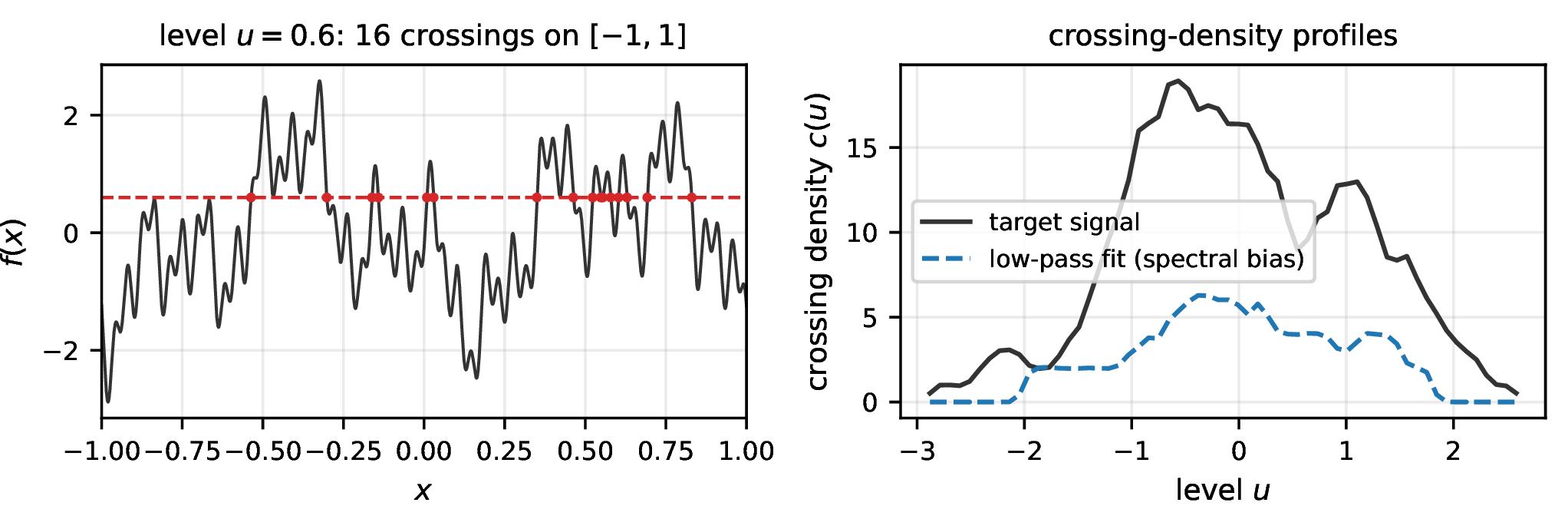
Let \(f:\Omega\subset\mathbb{R}^d\to\mathbb{R}\) be Lipschitz. For \(d=1\) and a level \(u\), let \(N_u(f;\Omega)\) be the number of solutions of \(f(x)=u\) in \(\Omega\). For stationary Gaussian processes, Rice’s formula 1 gives the expected crossing rate as a ratio of spectral moments: \(\lambda_0\) is the signal variance and \(\lambda_2\) the derivative variance, so \(\sqrt{\lambda_2/\lambda_0}\) is an RMS frequency. A field that lacks high-frequency energy crosses every level less often (Figure 2, right).
Two properties make the crossing density usable beyond the Gaussian setting. First, the Kac–Rice integrand: under mild conditions [25], \[\mathbb{E}\,N_u \;=\; \int_\Omega \mathbb{E}\bigl[\,\lvert f'(x)\rvert \,\big|\, f(x)=u\,\bigr]\, p_{f(x)}(u)\,dx ,\] which requires no stationarity. Second, and central for us, the deterministic co-area formula [26]: for Lipschitz \(f\) and integrable \(g\), \[\int_\Omega g\bigl(f(x)\bigr)\,\lVert\nabla f(x)\rVert\,dx \;=\; \int_{\mathbb{R}} g(u)\,\mathcal{H}^{d-1}\bigl(f^{-1}(u)\cap\Omega\bigr)\,du, \label{eq:coarea}\tag{3}\] where \(\mathcal{H}^{d-1}\) is the \((d{-}1)\)-dimensional Hausdorff measure. Taking \(g=\delta_\varepsilon(\cdot-u)\), a Gaussian kernel of bandwidth \(\varepsilon\), the left-hand side of 3 divided by \(\lvert\Omega\rvert\) becomes an \(\varepsilon\)-smoothed level-set density: crossings per unit length (\(d{=}1\)), level-set length per unit area (\(d{=}2\)), level-set area per unit volume (\(d{=}3\)). No probabilistic assumptions enter: 3 holds for the single deterministic field being fitted.
3.2 A differentiable Monte-Carlo estimator↩︎
Sampling coordinates \(x_1,\dots,x_N\) uniformly in \(\Omega\) (or using the given training coordinates) yields the estimator of 2 : \(\hat{c}_\varepsilon(u)=\frac{1}{N}\sum_i \delta_\varepsilon(f_\theta(x_i)-u)\,\lVert\nabla_x f_\theta(x_i)\rVert\) with \(\delta_\varepsilon(z)=(2\pi\varepsilon^2)^{-1/2}e^{-z^2/2\varepsilon^2}\). It is unbiased for the \(\varepsilon\)-smoothed level-set density and inherits the usual kernel trade-off: \(O(\varepsilon^2)\) smoothing bias across levels versus \(O(1/(N\varepsilon))\) variance. Three implementation points matter in practice.
Gradients are free and exact. \(\nabla_x f_\theta\) comes from automatic differentiation at arbitrary points; no finite differences, no grid. Backpropagating the loss through \(\lVert\nabla_x f_\theta\rVert\) is a double-backward operation, supported by all standard frameworks [27].
Levels at target quantiles. We place \(L\) levels \(u_1,\dots,u_L\) at uniformly spaced quantiles of the ground-truth values in the batch (between the 2nd and 98th percentile), which keeps every level populated regardless of the value histogram.
Same-batch targets. The target profile \(c^{\mathrm{gt}}(u_j)\) is the same estimator applied to the ground-truth values and gradient norms at the same batch points. Estimator and target then share sampling noise, which partially cancels in the difference—the loss compares two estimates of the same functional under the same measure, so even under non-uniform sampling both sides are biased identically toward densely sampled regions.
3.3 The Kac–Rice loss↩︎
The auxiliary loss matches the crossing-density profile at the \(L\) levels, normalized to be scale-free: \[\mathcal{L}_{\mathrm{KR}}(\theta) \;=\; \frac{1}{L} \sum_{j=1}^{L} \frac{\bigl(\hat{c}_\varepsilon(u_j) - c^{\mathrm{gt}}(u_j)\bigr)^2}{\bigl(c^{\mathrm{gt}}(u_j) + \bar c^{\mathrm{gt}}\bigr)^2}, \qquad \bar c^{\mathrm{gt}} = \tfrac1L\textstyle\sum_j c^{\mathrm{gt}}(u_j), \label{eq:loss}\tag{4}\] and the total objective is \(\mathcal{L}= \frac{1}{N}\sum_i (f_\theta(x_i)-y_i)^2 + \beta\,\mathcal{L}_{\mathrm{KR}}\). The normalization in 4 is not cosmetic: crossing densities grow linearly with frequency content, so the squared error grows quadratically, and an unnormalized version couples the effective weight \(\beta\) to the signal’s bandwidth. In early experiments the unnormalized loss with a weight tuned for one signal destabilized training on another; the relative form transfers across signals with a single \(\beta\).1
Defaults throughout: \(L=16\) levels, \(\varepsilon=0.15\,\sigma_y\) where \(\sigma_y\) is the standard deviation of the batch ground-truth values, and \(\beta=0.05\); all are ablated in Section 5.5.
3.3.0.1 What the loss constrains.
\(\mathcal{L}_{\mathrm{KR}}\) is a functional of the marginal level-set geometry: it pushes the field to have the right amount of level-crossing structure at each height, leaving where that structure goes to the reconstruction term. It cannot, alone, place an edge; it can insist that the total edge length at each gray level be right. This is weaker than a Fourier loss on a grid (which constrains amplitude at every frequency) but requires strictly less of the sampling process, and it is robust to pointwise target noise by construction: a zero-mean error of variance \(\sigma^2\) on individual gradient-norm targets perturbs each \(c^{\mathrm{gt}}(u_j)\) only at \(O(\sigma/\sqrt{N_j})\), with \(N_j\) the effective number of points near level \(j\), whereas a pointwise gradient-matching loss absorbs that noise at full variance.
3.3.0.2 Cost.
Relative to plain MSE, the additional cost is one backward pass for \(\nabla_x f_\theta\) (shared with any gradient-based loss) plus an \(O(NL)\) kernel evaluation, and double-backprop at
optimization time. In a back-to-back measurement (PE-MLP, \(16{,}384\) points, CPU; bench_timing.py in the released code, raw output in the result files), one training iteration took \(223\) ms with MSE only, \(473\) ms with the Kac–Rice term (\(2.12\times\)), and \(479\) ms with Sobolev (\(2.14\times\))—the two gradient-based losses share the dominant double-backward cost.
4 Estimator validation↩︎
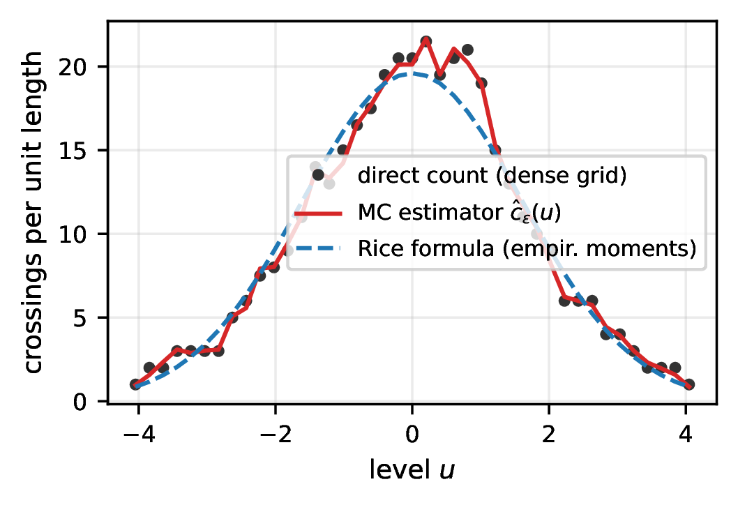
Before using 2 inside a loss we verify it in isolation (Figure 1). On deterministic multisine signals the estimator matches analytic crossing counts to within Monte-Carlo error (e.g., \(\sin(\pi k x)\) on \([-1,1]\) yields measured density \(k\pm2\%\) at \(N=2\times10^5\), and the 2D co-area version recovers the level-set length density of oriented gratings equally well). On an approximately Gaussian random field (60 random-phase sinusoids), the estimator agrees with direct sign-change counting on a dense grid within \(5\%\) across levels \(u\in[-2.5\sigma, 2.5\sigma]\), and with the Rice prediction 1 evaluated at empirical spectral moments within \(10\%\). These tests ship as unit tests with the code.
5 Experiments↩︎
5.1 Protocol↩︎
5.1.0.1 Backbones.
The primary backbone for loss comparisons is a ReLU MLP on Fourier positional encodings (PE-MLP; 3 hidden layers, width 256), the classic spectrally biased INR [7]. SIREN [1] and FINER [8] appear as architecture baselines under plain MSE, and we test composability by adding our loss to SIREN.
5.1.0.2 Baselines.
(i) MSE only; (ii) MSE + Focal Frequency Loss [14]—our implementation is numerically verified against the official package; (iii) MSE + normalized Sobolev (\(H^1\) gradient matching) [15], [16].
5.1.0.3 Tasks.
Regular grids (sanity check): a five-tone multisine in 1D (frequencies \(2,5,11,23,47\) half-cycles per unit) fitted from 1,024 grid points, and the camera image at \(128^2\). Scattered domains (the decisive test): the \(256^2\) camera image supervised only at \(N{=}8{,}192\) scattered locations (12.5% of
pixels) drawn from three densities—uniform (homogeneous), blobs (75% of samples in five Gaussian clusters), and ramp (linear density gradient)—plus a 1D variant and a synthetic multi-scale texture. On scattered tasks
all losses receive exactly the same information: the scattered pairs \(\{(x_i,y_i)\}\). FFL’s grid target is obtained by Delaunay-based linear interpolation (SciPy griddata [28]) and the loss is applied on random \(128^2\) crops of that grid each iteration (patch-based FFL, a mode the official
implementation supports); Sobolev and Kac–Rice gradient targets are central differences of that same interpolant sampled at the training points. Oracle-gradient variants (true image gradients; not legal supervision) isolate how much each
gradient-based method loses to interpolation noise.
5.1.0.4 Metrics.
PSNR on a dense evaluation grid; high-frequency PSNR (HF-PSNR: PSNR of the residual after removing a Gaussian low-pass, \(\sigma=4\) px); SSIM [29]; and relative spectral error in eight radial frequency bands. All results are mean \(\pm\) s.d.over three seeds (model initialization and, on scattered tasks, the sampling pattern). Adam [30] with cosine decay; full hyperparameters in Appendix 8.
5.2 Regular grids: parity, as expected↩︎
| 1D multisine | 2D camera \(128^2\) | |||
|---|---|---|---|---|
| 2-2(lr)3-5 Config | PSNR | PSNR | HF-PSNR | SSIM |
| MSE only | 70.64 \(\pm\) 0.11 | 40.52 \(\pm\) 1.10 | 42.46 \(\pm\) 1.10 | 0.97 \(\pm\) 0.00 |
| \(+\) FFL | 69.72 \(\pm\) 0.23 | 37.85 \(\pm\) 0.52 | 39.80 \(\pm\) 0.52 | 0.95 \(\pm\) 0.00 |
| \(+\) Sobolev | 70.41 \(\pm\) 0.22 | 29.30 \(\pm\) 0.12 | 31.26 \(\pm\) 0.12 | 0.90 \(\pm\) 0.00 |
| \(+\) Kac-Rice (ours) | 70.28 \(\pm\) 0.30 | 30.80 \(\pm\) 1.00 | 32.79 \(\pm\) 1.00 | 0.89 \(\pm\) 0.02 |
| SIREN (MSE) | 93.77 \(\pm\) 1.09 | 62.41 \(\pm\) 0.33 | 64.33 \(\pm\) 0.33 | 1.00 \(\pm\) 0.00 |
| FINER (MSE) | 73.57 \(\pm\) 7.68 | 139.72 \(\pm\) 3.09 | 141.56 \(\pm\) 3.04 | 1.00 \(\pm\) 0.00 |
5.2.0.1 1D: parity.
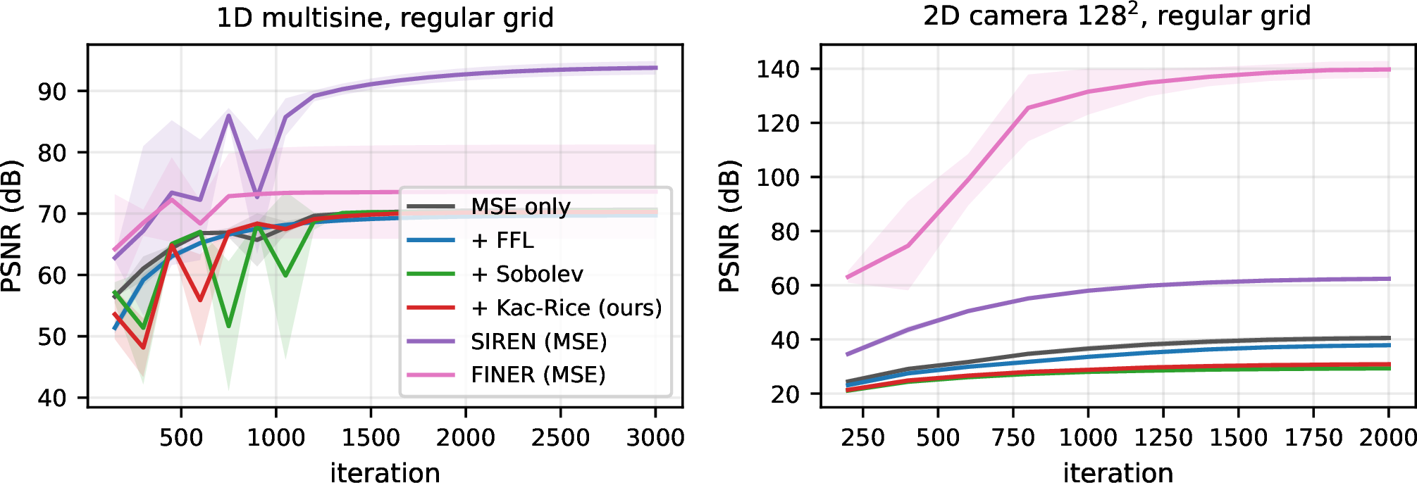
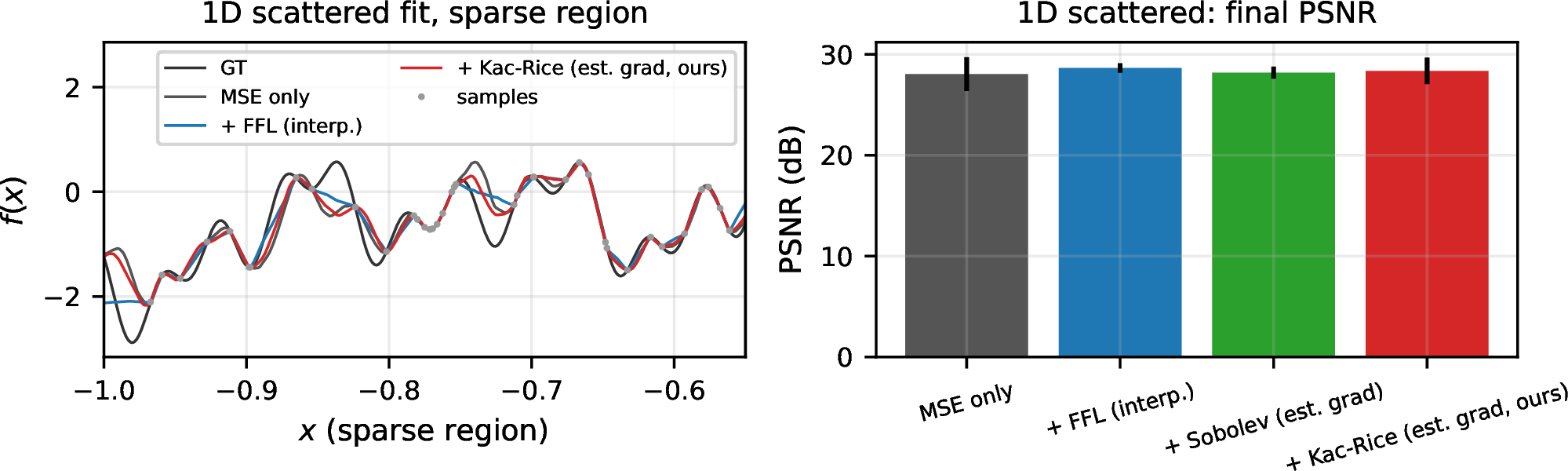
On the grid-sampled multisine, all four PE-MLP losses converge to statistically indistinguishable quality (MSE \(70.6\pm0.1\) dB, FFL \(69.7\pm0.2\), Sobolev \(70.4\pm0.2\), Kac–Rice \(70.3\pm0.3\)): with dense regular supervision, the reconstruction term alone eventually recovers all five tones, and no auxiliary drive changes the endpoint. SIREN, whose periodic activations match this signal family, reaches \(93.8\pm1.1\) dB; FINER reaches \(73.6\pm7.7\) dB with high seed variance. This is the expected sanity-check outcome: on-grid, auxiliary spectral losses neither help nor hurt materially in 1D.
5.2.0.2 2D: dense supervision does not need—and is hurt by—auxiliary drives.
On the \(128^2\) image (Table 1), MSE-only training is the best configuration (\(40.5\pm1.1\) dB); FFL costs \(2.7\) dB, and the two gradient-based losses cost \({\sim}10\) dB. The mechanism for the latter is instructive: the gradient targets are central differences of the discrete image, which are a low-pass-filtered version of the true local differences the MSE term is driving toward. At high fidelity the two objectives conflict, and a fixed \(\beta\) biases the optimum away from exact pixel reconstruction. (FFL’s target is the exact pixel grid, so it remains consistent with MSE and costs little.) [16] similarly report that Sobolev training for INRs requires care in how image derivatives are approximated. The architecture baselines put the loss family in perspective: on-grid, SIREN reaches \(62.4\pm0.3\) dB and FINER \(139.7\pm3.1\) dB (a numerically exact fit)—dense grid fitting is simply solved by activation engineering, and no auxiliary loss on a PE-MLP competes there. The practical reading, consistent with the few-shot literature [18]: auxiliary spectral objectives are tools for underdetermined regimes, not for dense overfitting, and we evaluate them where they are meant to operate—Section 5.3.
5.3 Scattered non-uniform domains: the decisive test↩︎
| blobs | ramp | uniform | ||||
|---|---|---|---|---|---|---|
| 2-3(lr)4-5(lr)6-7 Config | PSNR | HF-PSNR | PSNR | HF-PSNR | PSNR | HF-PSNR |
| griddata interp.(input) | 21.84 \(\pm\) 0.10 | 25.27 \(\pm\) 0.01 | 22.85 \(\pm\) 0.10 | 25.70 \(\pm\) 0.06 | 23.11 \(\pm\) 0.10 | 25.84 \(\pm\) 0.08 |
| MSE only | 18.88 \(\pm\) 0.12 | 22.76 \(\pm\) 0.02 | 19.73 \(\pm\) 0.09 | 22.89 \(\pm\) 0.07 | 20.18 \(\pm\) 0.07 | 23.19 \(\pm\) 0.05 |
| \(+\) FFL (interp.) | 21.62 \(\pm\) 0.12 | 25.01 \(\pm\) 0.05 | 22.48 \(\pm\) 0.12 | 25.31 \(\pm\) 0.09 | 22.73 \(\pm\) 0.11 | 25.46 \(\pm\) 0.09 |
| \(+\) Sobolev (est. grad) | 21.59 \(\pm\) 0.15 | 25.07 \(\pm\) 0.09 | 22.74 \(\pm\) 0.07 | 25.59 \(\pm\) 0.05 | 23.02 \(\pm\) 0.08 | 25.75 \(\pm\) 0.05 |
| \(+\) Kac-Rice (est. grad, ours) | 21.14 \(\pm\) 0.17 | 24.71 \(\pm\) 0.07 | 22.31 \(\pm\) 0.15 | 25.25 \(\pm\) 0.12 | 22.53 \(\pm\) 0.15 | 25.36 \(\pm\) 0.13 |
| \(+\) Sobolev (oracle grad) | 21.80 \(\pm\) 0.21 | 25.36 \(\pm\) 0.13 | – | – | – | – |
| \(+\) Kac-Rice (oracle grad) | 20.86 \(\pm\) 0.20 | 24.50 \(\pm\) 0.08 | – | – | – | – |
| SIREN (MSE) | 20.10 \(\pm\) 0.20 | 23.97 \(\pm\) 0.15 | – | – | – | – |
| SIREN \(+\) FFL (interp.) | 21.92 \(\pm\) 0.11 | 25.38 \(\pm\) 0.03 | – | – | – | – |
| SIREN \(+\) Sobolev (est. grad) | 21.50 \(\pm\) 0.14 | 25.06 \(\pm\) 0.10 | – | – | – | – |
| SIREN \(+\) Kac-Rice (ours) | 21.59 \(\pm\) 0.10 | 25.14 \(\pm\) 0.05 | – | – | – | – |
5.3.0.1 All auxiliary losses matter here; Kac–Rice ties FFL but does not beat it.
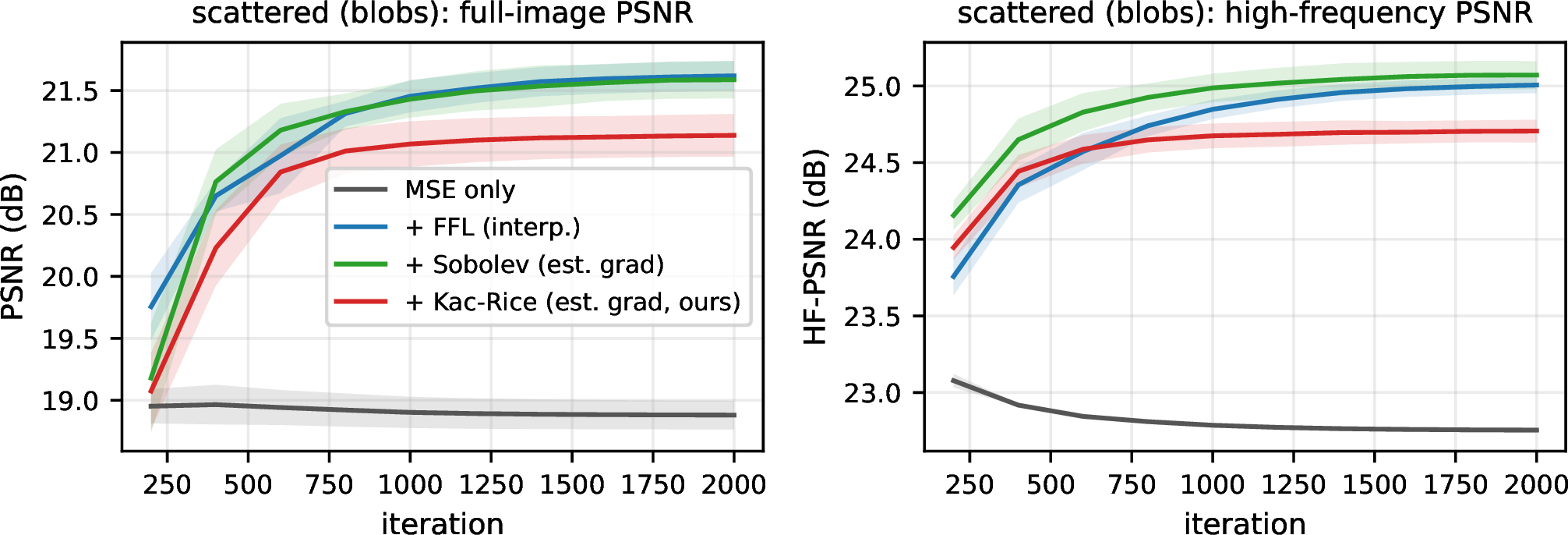
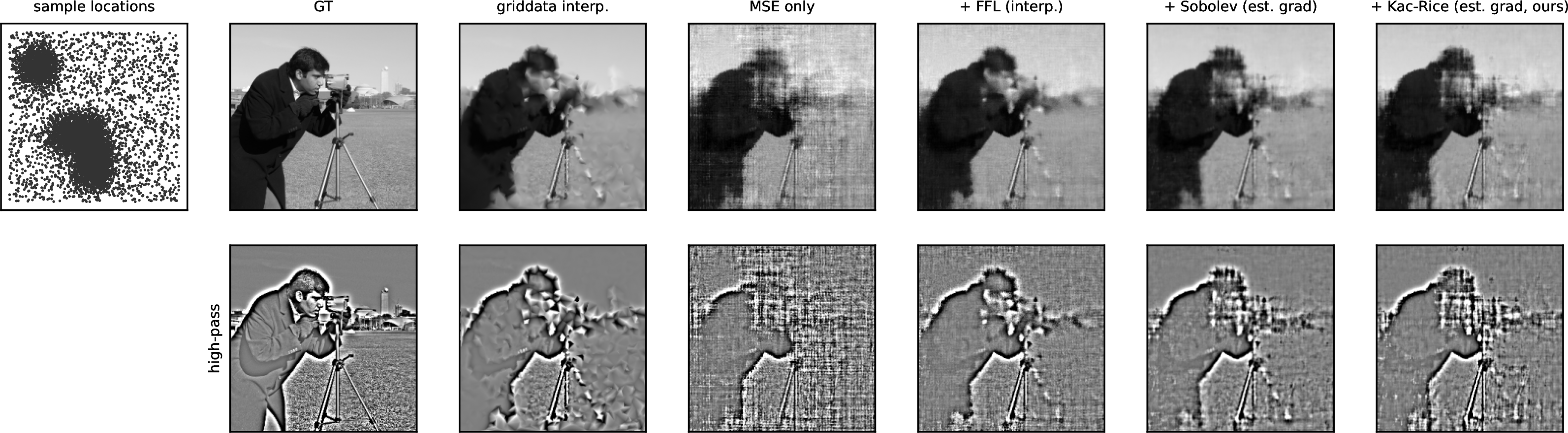
Table 2 is the decisive comparison, and we report it as measured. First, the regime change from Section 5.2 is dramatic: with scattered supervision, every auxiliary loss now adds \(+2.3\) to \(+3.0\) dB over MSE-only training (e.g.blobs: \(18.9\to21.1\)–\(21.6\) dB), and the qualitative gap is
larger than the numbers suggest—the MSE-only reconstructions in Figure 6 are blurred and streaked, while all three auxiliary variants recover coherent structure. Second, the central hypothesis of this paper is not
confirmed on the PE-MLP backbone: Kac–Rice lands within \(0.2\)–\(0.5\) dB of FFL-with-resampling on every sampling density (blobs \(21.1\)
vs.\(21.6\); ramp \(22.3\) vs.\(22.5\); uniform \(22.5\) vs.\(22.7\)) but does not overtake it, and the normalized Sobolev loss is the strongest or tied-strongest loss throughout. On SSIM the ordering partially reverses—Kac–Rice matches FFL on blobs and exceeds it on
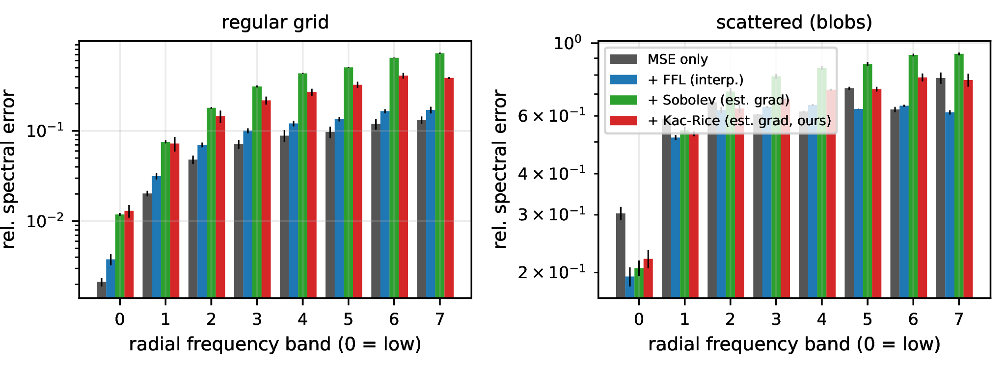
ramp and uniform (\(0.60/0.66/0.66\) vs.\(0.59/0.60/0.62\))—indicating the distributional loss buys structural coherence rather than pixel-wise accuracy; per-band
spectra (Figure 5, right) agree, with Kac–Rice showing the lowest error of the spatial-domain losses in the top two frequency bands. But the headline claim we set out to test—a clear PSNR win for crossing densities off-grid—did
not materialize.
5.3.0.2 The interpolation ceiling.
The griddata row of Table 2 is sobering context: at this sample budget, plain linear interpolation of the scattered samples scores within noise of the best INR configuration on PSNR (\(21.8\) on blobs). On the natural image, no loss studied here—frequency-domain or spatial—pushes a PE-MLP past the information ceiling that the interpolant itself sets (the texture task below is the sole, marginal
exception). What the INR adds over griddata is a compact, continuous, differentiable representation, not extra pixels; auxiliary losses determine how close to the ceiling one gets.
5.3.0.3 Content dependence: crossing statistics win on texture.
The synthetic multi-scale texture (Table 4) reverses the ordering. There Kac–Rice scores \(27.19\pm0.33\) dB (SSIM \(0.79\)) against FFL’s \(26.58\pm0.15\) (SSIM \(0.74\))—a \(+0.6\) dB advantage—with Sobolev at \(27.29\pm0.13\); the two spatial-domain losses match or
slightly exceed the griddata ceiling (\(26.96\)) while FFL stays below it. The pattern is theoretically coherent: the texture is statistically homogeneous, i.e.close to the stationary-random-field regime in
which crossing densities are an exact spectral functional 1 , whereas camera is edge-dominated and non-stationary, so its crossing profile is a blunter summary. Crossing-density supervision is at its best when the
signal looks like the random fields the theory was built for.
5.3.0.4 Oracle diagnostics: the distributional loss is robust to target smoothing.
Replacing estimated gradients with oracle image gradients helps Sobolev (\(21.6\to21.8\) dB) but does not help Kac–Rice (\(21.1\to20.9\) dB). This is the clearest direct evidence for the robustness mechanism of Section 3.3: Sobolev consumes gradient targets pointwise and benefits from their exactness, whereas Kac–Rice only consumes their batch statistics—smoothing noise largely cancels, and sharper targets, if anything, ask for crossing mass the MSE anchor cannot yet place. The practical consequence: Kac–Rice’s performance is insensitive to the quality of the gradient-estimation step, which is the step that is genuinely hard on scattered domains.
5.4 Composability with SIREN↩︎
Because the loss is orthogonal to architecture, it should stack with activation-based remedies. On the blobs task, SIREN+MSE scores \(20.10\pm0.20\) dB (SSIM \(0.56\));
adding Kac–Rice lifts it to \(21.59\pm0.10\) (SSIM \(0.65\)). To test whether this is specific to our loss we also ran SIREN with the two baseline auxiliaries: FFL reaches \(21.92\pm0.11\) (SSIM \(0.69\)) and Sobolev \(21.50\pm0.14\) (SSIM \(0.63\)). The honest conclusion is that composability is
a property of auxiliary spectral supervision in general, not of crossing densities in particular—though two details favor the distributional loss here: on SIREN, Kac–Rice edges Sobolev (the reverse of their PE-MLP ordering), and every SIREN+auxiliary
configuration beats its PE-MLP counterpart, so the loss and the activation fix address genuinely different parts of the problem.
5.5 Ablations↩︎
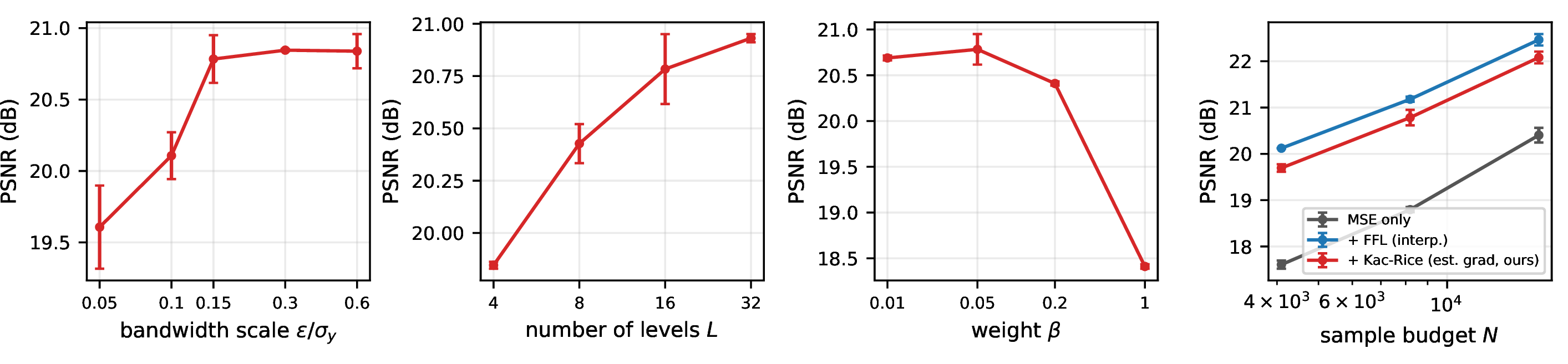
All ablations use camera/blobs at 1,000 iterations with 2 seeds (Figure 7); absolute numbers are therefore lower than in Table 2, and only relative sensitivity is
meaningful.
5.5.0.1 Bandwidth \(\varepsilon\).
The loss is robust for \(\varepsilon\ge0.15\,\sigma_y\) (PSNR \(20.8\)–\(20.9\) dB across \(\varepsilon/\sigma_y\in\{0.15,0.3,0.6\}\)) and degrades below it (\(19.6\) dB at \(0.05\)): a too-narrow Dirac starves most batch points of gradient signal, exactly the failure mode anticipated. The practical guidance is simply “not too small”—the nuisance parameter flagged at the outset turns out to have a wide plateau rather than a narrow sweet spot.
5.5.0.2 Number of levels \(L\).
Quality improves monotonically and saturates: \(19.9\), \(20.4\), \(20.8\), \(20.9\) dB for \(L=4,8,16,32\). Sixteen levels suffice.
5.5.0.3 Weight \(\beta\).
Performance is flat across \(\beta\in[0.01,0.2]\) (\(20.4\)–\(20.8\) dB) and collapses only at \(\beta=1\) (\(18.4\) dB), where the distributional term overwhelms reconstruction. The relative normalization of 4 is what makes this range transferable across signals.
5.5.0.4 Sample budget.
Across \(N\in\{4096, 8192, 16384\}\) the ordering is stable, with FFL ahead of Kac–Rice by a constant \({\sim}0.4\) dB (\(0.42/0.40/0.38\)). The auxiliary advantage over MSE is large at every budget but contracts slowly as sampling densifies—from \(+2.5/+2.1\) dB (FFL/Kac–Rice) at \(N{=}4096\) to \(+2.1/+1.7\) dB at \(N{=}16384\)—consistent with auxiliary drives mattering most when supervision is scarcest.
6 Discussion and limitations↩︎
6.0.0.1 What we learned.
Taking the experiments together, the honest verdict on the opening hypothesis is parity with a content-dependent edge, not a general victory: the crossing-density loss is a working, validated, mesh-free high-frequency drive that matches
frequency-domain and gradient-matching supervision on edge-dominated natural-image content, beats MSE-only training by large margins wherever supervision is scarce, and overtakes FFL only where the signal is statistically homogeneous (texture)—the regime
the underlying theory is actually about. Its remaining distinguishing properties are structural. First, it is the only loss in the comparison that needs neither a grid at any point in the pipeline (FFL needs one for its transform) nor trustworthy pointwise
gradient targets (Sobolev’s accuracy tracks target quality, while Kac–Rice is insensitive to it—the oracle diagnostic). Second, it buys structural metrics preferentially: SSIM matching (blobs) or exceeding (ramp,
uniform) FFL’s, and the best top-band spectral error among the spatial-domain losses, at a small PSNR cost. Where those structural properties are decisive—supervision without any usable grid, gradient targets too noisy to match pointwise—it is
a reasonable default; where a grid or clean gradients exist, existing losses are already sufficient.
6.0.0.2 Why no win?
The mechanism we can defend from the data: the crossing profile constrains \(L\) numbers per batch—a far weaker constraint than FFL’s full spectrum or Sobolev’s \(N\) pointwise gradients. Robustness and weakness here are two faces of the same statistic. The interpolation-ceiling observation sharpens this: at \(N{=}8{,}192\) samples all auxiliary losses already saturate what linear interpolation extracts from the samples, so there was little headroom for a cleverer loss to express an advantage. Regimes where the ceiling itself moves—strong shape priors, composed losses, or targets (b)-style scheduled crossing profiles that inject prior spectral knowledge rather than re-encoding sample information—are where a distributional drive could still separate; all remain untested here.
6.0.0.3 Limitations.
(i) Scope: 1D signals and 2D images only; neural SDFs from point clouds—arguably the setting where “no grid, noisy normals” bites hardest—and few-shot NeRF remain future work, and our conclusions should not be extrapolated to them. (ii) The loss
constrains distributional level-set geometry, not phase: it cannot place an edge, only demand total edge mass, so it is strictly an auxiliary term. (iii) Hyperparameters are benign but real: \(\varepsilon\) has a wide
plateau above \(0.15\sigma_y\), \(L{=}16\) suffices, and \(\beta\) tolerates a \(20\times\) range—but all were tuned on the
same image family used for evaluation. (iv) Double backprop makes each iteration \({\sim}2.1\times\) an MSE iteration, matching Sobolev. (v) Evaluation uses one natural test image plus one synthetic texture at one
resolution per task; broader image suites would tighten the estimates, though the seed-level spreads are already small relative to the effects discussed. (vi) camera is a standard public test image; no personal or sensitive data is
involved.
7 Conclusion↩︎
We turned the Rice level-crossing density into a differentiable, mesh-free, FFT-free auxiliary loss for INRs, validated the underlying estimator against exact crossing counts and the Rice formula, and evaluated it against the strongest loss-based alternatives under strict information parity. The result is a clean, honest data point for the field: crossing statistics work as a high-frequency drive—recovering \(+2.3\)–\(3.0\) dB over plain reconstruction on PE-MLP and \(+1.4\)–\(1.8\) dB on SIREN wherever supervision is scarce—but on natural images they match rather than beat frequency-domain and Sobolev supervision, pulling ahead of the frequency-domain loss only on statistically homogeneous texture, with their broader distinction being structural: no grid, no FFT, and demonstrated insensitivity to gradient-target noise. The broader point is that the geometry of level sets offers a family of spatial-domain spectral surrogates—crossing densities here; critical-point counts and Euler characteristics of excursion sets [24] are natural sequels—that remain defined exactly where frequency-domain tooling is not, and the settings that motivated this loss most strongly (point-cloud SDFs, scheduled crossing targets) remain open.
7.0.0.1 Reproducibility.
Code, experiment scripts, raw result JSONs, and the estimator’s unit tests are public at https://github.com/gunnerhowe/Research (directory kac-rice). All experiments were run
on a single consumer workstation (16-core CPU / RTX 3080); the complete suite reproduces in under a day of commodity compute.
8 Hyperparameters↩︎
| Backbone (loss comparisons) | PE-MLP: ReLU, 3 hidden layers, width 256 |
| Positional encoding | \(\{\sin,\cos\}(2^k\pi x)\), \(k=0..5\) (1D), \(k=0..7\) (2D) |
| SIREN / FINER | width 256, 3 hidden layers, \(\omega_0=30\); FINER default init |
| Optimizer | Adam, lr \(10^{-3}\) (PE-MLP) / \(5\times10^{-4}\) (SIREN, FINER) |
| Schedule | cosine decay to \(0.05\times\) lr |
| Iterations | 3,000 (1D), 2,000 (2D), 1,000 (ablations); full batch |
| Kac–Rice loss | \(L=16\) levels at quantiles \([0.02,0.98]\); \(\varepsilon=0.15\sigma_y\); \(\beta=0.05\) |
| Sobolev loss | normalized \(H^1\); weight \(0.05\) |
| FFL | \(\alpha=1\), weight \(1.0\); random \(128^2\) crops on scattered tasks |
| Scattered supervision | \(N=8{,}192\) samples of the \(256^2\) image (12.5%) |
| Seeds | 3 (init + sampling pattern); 2 for ablations |
9 Reproducibility↩︎
All code, raw result JSONs, and figure generators are public at https://github.com/gunnerhowe/Research (directory kac-rice). Every number and figure in this paper regenerates
from the released raw runs; no result exists only in the manuscript.
9.0.0.1 Environment.
Python 3.13.6, PyTorch 2.7.1, NumPy 2.4.4, SciPy 1.17.0, Matplotlib 3.10.7, on a single 16-core Windows workstation. All headline experiments ran on CPU in float32 (the machine’s GPU was shared with unrelated jobs; CPU wall-clock is not a reported metric, and the timing comparison of Section 3 uses the dedicated back-to-back benchmark below).
9.0.0.2 Commands.
Estimator correctness tests: python tests/test_correctness.py (7 tests: crossing counts, co-area, Rice agreement, FFL parity vs.the official package, gradient flow). Full experiment suite (parallel workers; resume-safe, so a single
sequential invocation is equivalent):
python experiments/run_paper.py –suites exp1_1d exp2_1d exp1_2d
python experiments/run_paper.py –suites exp2_2d –tag _a
python experiments/run_paper.py –suites ablations –tag _c
Figures and tables: python experiments/make_figures.py reads results/paper/*.json and writes every figure and LaTeX table used here. Timing artifact: python experiments/bench_timing.py writes
results/paper/timing.json (source of the \(2.12\times\)/\(2.14\times\) factors).
9.0.0.3 Seeds and scope.
Seeds \(0\)–\(2\) everywhere (model init and, on scattered tasks, sampling patterns), \(0\)–\(1\) for ablations; all seeds are set by CLI and recorded per run in the JSONs. Total compute: under one day on the single workstation.
10 Additional results↩︎
| Config | PSNR | HF-PSNR | SSIM |
|---|---|---|---|
| MSE only | 24.81 \(\pm\) 0.88 | 19.78 \(\pm\) 0.80 | 0.59 \(\pm\) 0.06 |
| \(+\) FFL (interp.) | 26.58 \(\pm\) 0.15 | 21.64 \(\pm\) 0.15 | 0.74 \(\pm\) 0.01 |
| \(+\) Sobolev (est. grad) | 27.29 \(\pm\) 0.13 | 22.23 \(\pm\) 0.22 | 0.81 \(\pm\) 0.01 |
| \(+\) Kac-Rice (est. grad, ours) | 27.19 \(\pm\) 0.33 | 22.17 \(\pm\) 0.10 | 0.79 \(\pm\) 0.02 |
References↩︎
The same reasoning applies to the Sobolev baseline, which we normalize by the mean squared ground-truth gradient norm; without this, its useful weight range also varies by orders of magnitude across signals.↩︎