Contextual Procurement Auctions with Bandit Learning
July 07, 2026
Abstract
We study repeated contextual procurement auctions in which the platform must learn context-dependent product values from bandit feedback. We give an exactly truthful explore-then-commit mechanism with \(\widetilde{O}((ng)^{1/3}T^{2/3})\) regret. We also give a frozen-payment UCB mechanism with a regret-incentive tradeoff: the near-UCB tuning attains \(\widetilde{O}(\sqrt{ngT})\) welfare regret, while for fixed \(n,g\) its total incentive error is \(\widetilde{O}(T^{3/4})\); the balanced tuning gives \(\widetilde{O}(T^{2/3})\) on both scales. Regret is measured as welfare loss relative to the full-information efficient allocation. We prove a matching lower bound for the frozen-payment regret-incentive tradeoff.
1 Introduction↩︎
Auctions are often used not merely to extract revenue, but to allocate scarce resources whose productive value is initially uncertain [1]; see also the standard auction-theory treatments of Milgrom [2] and Krishna [3]. A useful historical example is the leasing of the Laurion silver mines in classical Athens. The surviving Athenian records document leases and public sales administered by the poletai, the official sellers, and modern studies of these inscriptions show that the leased mines varied by location, history, classification, and price [4]–[6]. From a modern allocation perspective, a mining lease was not a known object with a fixed value. Its realized value depended on geological conditions, prior excavation, nearby discoveries, extraction technology, operating costs, and the state of silver demand. Selling a lease to the highest bidder could raise public revenue, but it need not allocate the right to the operator who would generate the greatest total surplus.
This example suggests a counterfactual design question that is still central today: how should a public operator allocate resources when the welfare contribution of each allocation is context-dependent and must be learned over time? A modern mechanism could deliberately explore under-sampled mine categories, use realized production as bandit feedback about productivity, and then allocate future rights using estimates of surplus rather than payments alone. The loss from early mistakes would be measured not only by foregone lease revenue, but by the cumulative social value lost from allocating public assets without knowing which operator can use them best. This is the lens of welfare regret: the gap between the welfare achieved by an online mechanism and the welfare that would have been achieved by an oracle that knew the true context-value relationship.
The same structure appears in contemporary infrastructure markets. Electricity markets are the leading example. System operators repeatedly procure and dispatch generation, storage, and demand response under contexts such as seasonality, weather, renewable output, fuel prices, congestion, and industrial load. The canonical spot-pricing and network-pricing literature treats efficient dispatch as an optimization of social surplus or system cost, with prices used to coordinate incentives rather than as the operator’s final objective [7], [8]; transmission pricing raises the same welfare-coordination issue in network form [9]. Similar issues arise in computational infrastructure. The growth of large language models has made compute allocation and model selection strongly context dependent: the value of assigning scarce GPU or inference capacity depends on task complexity, latency requirements, quality requirements, and provider costs. This connects to a broader literature on allocating heterogeneous computational resources [10]. Recent work explicitly models LLM provider selection as a reverse contextual bandit auction [11]. Emissions permit markets provide another example. Cap-and-trade systems create scarce rights to emit, and the economic objective is to meet environmental constraints at low social cost rather than simply to maximize auction proceeds [12], [13]. Auction design for such permits then becomes a means of allocating scarce environmental rights efficiently [14], [15].
We study a repeated contextual procurement auction that captures the procurement side of these allocation problems. There are \(n\) producers and a finite set of contexts. Producer \(i\) has a private cost \(k_i\). When producer \(i\) is selected in context \(c\), the platform obtains an unknown gross value with mean \(\mu_{i,c}\), observes only the selected producer-context outcome, and learns from this bandit feedback. Under truthful bidding, the social surplus of selecting \(i\) in context \(c\) is \(\mu_{i,c}-k_i\), and the outside option has surplus zero. The full-information benchmark is the efficient procurement mechanism that knows \(\mu\) and, in each context, selects the producer with the largest nonnegative surplus. Our goal is to design learning mechanisms with low welfare regret while controlling strategic incentives.
First, we formulate contextual procurement with private costs and unknown context-dependent values, using total-surplus regret as the performance measure. Second, we show that the natural UCB procurement allocation rule achieves \(\widetilde{O}(\sqrt{ngT})\) regret under truthful bidding. Third, we give an explore-then-commit mechanism whose exploration phase is bid-independent and whose commit phase uses empirical VCG-style critical payments; this mechanism is exactly dominant-strategy truthful and achieves \(\widetilde{O}((ng)^{1/3}T^{2/3})\) regret. Fourth, we introduce a frozen-payment UCB mechanism that separates payment learning from adaptive allocation learning. Its near-UCB tuning obtains regret \(\widetilde{O}(\sqrt{ngT})\), while its approximate-truthfulness guarantee follows a quantitative tradeoff with the payment-exploration error; the balanced tuning gives \(\widetilde{O}(T^{2/3})\) regret and incentive error for fixed \(n,g\). Finally, we prove a lower bound showing that the frozen-payment regret-incentive tradeoff is essentially unavoidable.
2 Related Work↩︎
Our full-information benchmark is the efficient single-parameter procurement mechanism, implemented by critical payments as in the standard VCG tradition; this tradition originates in Vickrey’s auction model [1], Clarke’s pivotal mechanism [16], and Groves mechanisms [17]. We refer to [18] for algorithmic mechanism-design background. This benchmark contrasts with Myerson’s optimal auction theory, where expected revenue is characterized by virtual values or virtual costs [19]; see also [2], [3]. The distinction is important for our motivation: virtual values and virtual costs are useful analytic transformations for characterizing optimal mechanisms, but regret measured in these transformed quantities is not a primitive economic loss such as welfare loss, payment loss, or buyer-surplus loss along the allocation path. Our regret is instead measured directly in expected surplus \(\mu_{i,c}-k_i\). Our approximate-incentive guarantees are also related to the broader study of approximately incentive compatible mechanisms [20], although our bounds arise from online learning and frozen payment estimation. Our single-unit procurement model is deliberately simpler than structured or capacitated procurement settings, where feasibility constraints and multi-unit supply create additional allocation structure [21], [22].
The learning side of our model is closest to stochastic bandits and UCB-style allocation rules, starting from sequential experimental design [23] and asymptotically efficient allocation [24], with UCB giving finite-time guarantees [25]; see also the survey of Bubeck and Cesa-Bianchi [26]. Contextual bandit algorithms extend this framework by using side information before allocation [27], [28]. Applied and linear variants provide standard contextual benchmarks [29], [30], with confidence-set methods for linear stochastic bandits also central [31]. In strategic bandit allocation, however, the learning path depends on bids, so monotonicity and payment computation are substantially more delicate. Babaioff, Sharma, and Slivkins characterized truthful multi-armed-bandit mechanisms and showed a fundamental cost of truthfulness for deterministic mechanisms [32]. Devanur and Kakade studied truthful pay-per-click auctions with unknown click rates [33]. Babaioff, Kleinberg, and Slivkins later used random resampling to obtain truthful-in-expectation mechanisms from monotone allocation rules while retaining near-optimal bandit regret [34]. Our mechanisms take a different route: exact truthfulness is obtained through bid-independent explore-then-commit, while the lower-regret UCB variant freezes payment estimates to obtain approximate truthfulness. Related incentive-aware bandit mechanisms have also been studied in crowdsourcing [35] and expertsourcing [36], as well as smart-grid demand response [37]. Strategic combinatorial bandit mechanisms build on the broader combinatorial bandit framework [38], [39].
Several recent papers combine contextual learning with auctions. Abhishek, Jain, and Gujar study truthful contextual multi-armed bandits for sponsored search auctions [40]. Zhang and Luo study contextual second-price pay-per-click auctions with the goal of minimizing revenue regret relative to an oracle with perfect click-through-rate predictions [41]. The closest recent work to our setting is that of Patra, Damle, Padala, and Gujar, who study truthful reverse auctions for adaptive LLM provider selection via contextual MABs [11].2 Their regret is defined relative to an optimal reverse-auction benchmark based on Myerson-style virtual costs. This is a natural surrogate for analyzing that mechanism-design objective, but virtual-cost regret has no direct realized economic interpretation: virtual costs include distributional information-rent corrections and are not the agents’ actual costs. A small virtual-cost regret therefore need not mean small welfare loss, payment loss, or buyer-surplus loss on the realized allocation path. Our objective is different: we target welfare regret relative to the efficient surplus benchmark. This difference matters in infrastructure settings where the operator acts as a planner and payments are primarily instruments for elicitation and coordination.
3 Model and Full-Information Benchmark↩︎
We study a repeated contextual procurement problem with unknown product values. There are \(n\) producers, indexed by \(i\in[n]\). Producer \(i\) owns a single product \(a_i\), whose context-dependent gross value is unknown to the platform and must be learned from bandit feedback.
Producer \(i\) has private production cost \(k_i\in[0,1]\). At the beginning of the interaction, producer \(i\) submits an ask bid \(b_i\in[0,1]\), which remains fixed throughout the horizon. Truthful bidding means \(b_i=k_i\).
There is a finite context set \(\mathcal{C}=\{1,\dots,g\}\). At each round \(t=1,\dots,T\), a context \(c_t\in\mathcal{C}\) is observed. The context process is exogenous and action-independent. It may be stochastic and depend on prior contexts, but its conditional law is unaffected by bids, allocations, reward realizations, or mechanism randomization. In particular, changing a producer’s report does not change the law of future contexts.
Let \(\mathcal{F}_{t-1}\) be the history immediately before context \(c_t\) is observed. If product \(a_i\) is selected in context \(c\), the platform observes a bounded random outcome \(Y_t(i)\in[0,1]\) with \(\mathbb{E}[Y_t(i)\mid \mathcal{F}_{t-1},c_t=c]=\mu_{i,c}\). Thus, for every adaptively selected producer–context pair, the centered observations form a bounded martingale-difference sequence. This conditional mean assumption, rather than a mean conditional only on the current context, is what permits the uniform UCB concentration bounds below. The unknown mean matrix is \(\mu=\{\mu_{i,c}\}_{i\in[n],c\in\mathcal{C}}\). The platform observes only bandit feedback: after choosing \(i_t\), it observes \(Y_t(i_t)\) and does not observe the counterfactual outcomes of other products.
If producer \(i\) is selected and paid \(p_{i,t}\), its realized utility is \(p_{i,t}-k_i\). The realized social surplus contribution is \(Y_t(i)-k_i\).
The learning objective in this paper is welfare-maximizing efficient procurement under truthful costs. Payments are used to control incentives, while regret is measured against the full-information efficient allocation; see Vickrey [1], Clarke [16], Groves [17], and the textbook treatment in [18].
Throughout the note, all tie-breaking rules are fixed ex ante and independent of the submitted bids.
For readability, the proofs are deferred to Appendix 10.
3.1 Full-Information Benchmark↩︎
We first define the benchmark mechanism that knows the true value matrix \(\mu\). For a bid profile \(b=(b_1,\dots,b_n)\) and context \(c\), define producer \(i\)’s score as \(S_i(c;b)=\mu_{i,c}-b_i\). The outside option \(\emptyset\) has score \(S_{\emptyset}(c;b)=0\). The full-information efficient procurement allocation rule chooses \[a^\star(c;b) \in \arg\max_{a\in[n]\cup\{\emptyset\}} S_a(c;b).\] Equivalently, the platform procures from a producer only when the largest score is nonnegative.
For producer \(i\), define the competing threshold and the full-information VCG critical payment by \[H_i(c;b_{-i}) = \max\left\{ 0, \max_{j\neq i} \left(\mu_{j,c}-b_j\right) \right\},\] and \[q_i^\star(c;b_{-i}) = \left[ \mu_{i,c}-H_i(c;b_{-i}) \right]_{[0,1]},\] where \([x]_{[0,1]}=\min\{1,\max\{0,x\}\}\). If producer \(i\) is selected, the platform pays \(q_i^\star(c;b_{-i})\). If producer \(i\) is not selected, it receives zero.
Because the score \(\mu_{i,c}-b_i\) is strictly decreasing in \(b_i\) and tie-breaking is fixed ex ante, the allocation rule is monotone nonincreasing in \(b_i\): a producer who reports a higher cost is weakly less likely to be selected. The critical-payment rule therefore implements the full-information efficient allocation truthfully, as in the VCG/critical-value tradition of Vickrey [1], Clarke [16], and Groves [17].
Proposition 1 (Full-information truthfulness and individual rationality). The full-information efficient allocation rule with the critical payments above is dominant-strategy truthful and ex-post individually rational.
Under truthful bidding, the full-information benchmark is \[\mathrm{OPT}(T) = \sum_{t=1}^T \max\left\{ 0, \max_{i\in[n]} \left(\mu_{i,c_t}-k_i\right) \right\}.\] For any learning allocation rule that selects \(i_t\in[n]\cup\{\emptyset\}\) at round \(t\), define its regret under truthful bidding by \[\begin{align} B_t &:= \max\left\{0,\max_{i\in[n]}(\mu_{i,c_t}-k_i)\right\},\\ \mathrm{Reg}(T) &:= \sum_{t=1}^T \left[ B_t - \mathbf{1}\{i_t\neq\emptyset\} (\mu_{i_t,c_t}-k_{i_t}) \right]. \end{align}\]
This regret notion compares the learning allocation directly with the full-information efficient allocation under truthful costs.
4 Explore-Then-Commit↩︎
We first define an explore-then-commit (ETC) mechanism. It separates learning from strategic allocation: the platform explores using a bid-independent rule, freezes the resulting value estimates, and then runs the efficient critical-price mechanism for the empirical instance. This gives a slower regret rate than UCB allocation, but it gives exact dominant-strategy truthfulness.
Let \(M\in\{1,\dots,T\}\) be the exploration length.
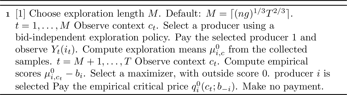
Exploration phase. For the first \(M\) rounds, the platform uses a bid-independent exploration policy. Both the exploration allocation rule and the exploration payments are assumed to be independent of the submitted bids. To ensure individual rationality during exploration, the exploration payment to a selected producer is set to \(1\) (or any other bid-independent constant \(\ge \max_i k_i\)); since this payment is bid-independent, it does not affect incentive compatibility. Let \(N^0_{i,c}\) be the number of observations of pair \((i,c)\) during exploration, and let \(\widehat\mu^0_{i,c}\) be the corresponding empirical mean.
Commit phase. After exploration, the estimates \(\widehat\mu^0\) are frozen. In each round \(t>M\), define \(\widehat S_i^0(c;b)=\widehat\mu^0_{i,c}-b_i\) for \(i\in[n]\) and \(\widehat S_{\emptyset}^0(c;b)=0\). The mechanism chooses \(i_t\in\arg\max_{a\in[n]\cup\{\emptyset\}}\widehat S_a^0(c_t;b)\). For the selected producer \(i_t=i\), define \(\widehat H_i^0(c_t;b_{-i})=\max\{0,\max_{j\neq i}(\widehat\mu^0_{j,c_t}-b_j)\}\) and pay the empirical VCG critical payment \(\widehat q^0_i(c_t;b_{-i})=[\widehat\mu^0_{i,c_t}-\widehat H_i^0(c_t;b_{-i})]_{[0,1]}\). If no producer is selected, no payment is made.
Assumption 1 (Uniform exploration coverage). There exists a constant \(c_{\mathrm{cov}}>0\) such that, with probability at least \(1-(Tng)^{-2}\), \[N^0_{i,c} \ge c_{\mathrm{cov}}\frac{M}{ng} \qquad \text{for all }(i,c)\in[n]\times\mathcal{C}.\] This is a joint coverage condition on the exogenous context process and the bid-independent exploration policy: during the exploration phase, each context must occur sufficiently often, and conditional on each context, the exploration policy must sample each producer sufficiently often. In particular, this assumption is nonvacuous only when \(M\) is at least of order \(ng\) (and typically \(ng\log(Tng)\) for high-probability coverage).
Remark 2 (A sufficient coverage condition). If the contexts are i.i.d. with \(\mathbb{P}(c_t=c)\ge\pi_{\min}>0\) for every \(c\), and exploration selects each producer uniformly and independently of bids, then Chernoff bounds give Assumption 1 with \(c_{\mathrm{cov}}=g\pi_{\min}/2\), provided \(M\ge C_0(n/\pi_{\min})\log(Tng)\) for a sufficiently large universal constant \(C_0\).
Theorem 3 (Explore-then-commit regret). Under the conditional reward assumption in the model, Assumption 1, and truthful bidding, the explore-then-commit procurement mechanism satisfies \[\mathbb{E}\!\left[\mathrm{Reg}(T)\right] = \widetilde{O}\!\left( M + T\sqrt{\frac{ng}{M}} \right).\] Choosing \(M\asymp(ng)^{1/3}T^{2/3}\) gives \(\mathbb{E}[\mathrm{Reg}(T)] =\widetilde{O}((ng)^{1/3}T^{2/3})\), which is \(\widetilde{O}(T^{2/3})\) for constant \(n\) and \(g\). Thus, for fixed \(n\) and \(g\), ETC has \(\widetilde{O}(T^{2/3})\) welfare regret.
Theorem 4 (Truthfulness of explore-then-commit). Suppose the exploration allocation rule and exploration payments are bid-independent, the commit-phase allocation and payments are computed from the frozen exploration estimates \(\widehat\mu^0\), and tie-breaking is fixed ex ante and bid-independent. Then the explore-then-commit procurement mechanism is dominant-strategy truthful. With the exploration payment set to \(1\), it is also ex-post individually rational.
Combining Theorems 3 and 4, for fixed \(n\) and \(g\), ETC has \(\widetilde{O}(T^{2/3})\) welfare regret and zero incentive error.
5 Frozen-Payment UCB↩︎
We next study a mechanism that keeps the adaptive allocation power of UCB but freezes the payment rule after an initial bid-independent exploration phase. We first recall the UCB allocation rule that drives the post-exploration allocation.
For each pair \((i,c)\), let \(N_{i,c}(t)\) be the number of observations of producer \(i\) in context \(c\) before round \(t\), and let \(\widehat\mu_{i,c}(t)\) be the corresponding empirical mean. We use the convention \(\widehat\mu_{i,c}(t)=0\) whenever \(N_{i,c}(t)=0\). Define \[\beta_{i,c}(t) = \sqrt{ \frac{C\log(2Tng)}{N_{i,c}(t)\vee1} },\] where \(C\ge 1\) is a sufficiently large universal constant. Unobserved pairs are optimistic by construction, and on observed pairs optimism holds on the UCB concentration event below. We state the results for known horizon \(T\); a standard doubling schedule removes this knowledge at an additional logarithmic factor.
Given bids \(b\), define the optimistic UCB scores by \(\widetilde{S}_i(c;b,t)=\widehat\mu_{i,c}(t)+\beta_{i,c}(t)-b_i\) for \(i\in[n]\) and \(\widetilde{S}_{\emptyset}(c;b,t)=0\). The UCB procurement allocation rule chooses \(i_t\in\arg\max_{a\in[n]\cup\{\emptyset\}}\widetilde{S}_a(c_t;b,t)\).
Proposition 5 (UCB regret). Suppose the bounded conditional-mean assumption in the model holds for every adaptive history and every producer–context pair. Under truthful bidding \(b_i=k_i\), the UCB procurement allocation rule satisfies \[\mathbb{E}\!\left[\mathrm{Reg}(T)\right] \le 4\sqrt{CngT\log(2Tng)} +O\!\left(\frac{1}{Tn^2g^2}\right).\] In particular, if \(n\) and \(g\) are constants, then \(\mathbb{E}[\mathrm{Reg}(T)]=\widetilde{O}(T^{1/2})\).
Proposition 5 gives the sharper welfare-regret benchmark. However, unlike the explore-then-commit mechanism, the UCB allocation path is adaptive and bid-dependent. A producer’s bid may affect early allocations, which then affects future sample counts, empirical means, UCB bonuses, and future allocations. Thus dynamic truthfulness does not follow directly from applying per-round critical payments.
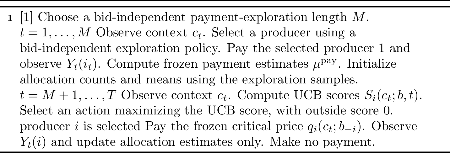
We analyze a UCB mechanism with frozen payments. The mechanism first runs a bid-independent exploration phase of length \(M\) (with bid-independent exploration payments, e.g.\(1\) per selected producer per round, as in the ETC mechanism). It computes payment estimates \(\widehat\mu^{\mathrm{pay}}\) using only this initial exploration data and then freezes them. Later observations are used only for allocation learning and are not used to compute payments. The allocation-learning estimates \(\widehat\mu_{i,c}(t)\) may be initialized with the same bid-independent exploration samples, but the payment estimates \(\widehat\mu^{\mathrm{pay}}\) are frozen after exploration and are never updated.
The key point is that frozen payments remove the direct dependence of producer \(i\)’s payment on its own bid and on the later UCB learning path. Producer \(i\)’s bid can still affect whether it is selected, and hence can affect the future UCB allocation history, but whenever \(i\) is selected in context \(c\), its payment is the frozen critical payment \(\widehat q_i(c;b_{-i})\), which depends only on the frozen payment estimates, the context, and the other producers’ bids.
5.1 Frozen Payment Rule and Regret↩︎
Given frozen payment estimates \(\widehat\mu^{\mathrm{pay}}\), define \[\begin{align} \widehat H_i(c;b_{-i}) &= \max\{0,\max_{j\neq i}(\widehat\mu^{\mathrm{pay}}_{j,c}-b_j)\},\\ \widehat q_i(c;b_{-i}) &= [\widehat\mu^{\mathrm{pay}}_{i,c}-\widehat H_i(c;b_{-i})]_{[0,1]} . \end{align}\] If producer \(i\) is selected in context \(c\), it is paid \(\widehat q_i(c;b_{-i})\). If it is not selected, it receives zero.
The UCB allocation rule still uses adaptive UCB estimates. At round \(t>M\), with context \(c_t\), it uses the scores \[\widetilde{S}_i(c_t;b,t)=\widehat\mu_{i,c_t}(t)+\beta_{i,c_t}(t)-b_i, \qquad \widetilde{S}_{\emptyset}(c_t;b,t)=0 .\] It then chooses \(i_t\in\arg\max_{a\in[n]\cup\{\emptyset\}}\widetilde{S}_a(c_t;b,t)\). The observations collected after the initial exploration phase are used to update \(\widehat\mu_{i,c}(t)\) and \(\beta_{i,c}(t)\) for allocation learning only; they are not used to update the frozen payments.
Theorem 6 (Regret of frozen-payment UCB). Under truthful bidding and the bounded conditional-mean assumption, the frozen-payment UCB mechanism with any \(M\)-round bid-independent exploration phase, whose allocation estimates are initialized with the exploration observations, satisfies \[\mathbb{E}\!\left[\mathrm{Reg}(T)\right] = \widetilde{O}\!\left(M+\sqrt{ngT}\right).\] In particular, for fixed \(n\) and \(g\), the near-UCB tuning achieves \(\mathbb{E}[\mathrm{Reg}(T)]=\widetilde{O}(T^{1/2})\), while the balanced tuning gives \(\mathbb{E}[\mathrm{Reg}(T)]=\widetilde{O}(T^{2/3})\); the role of the balanced tuning appears in the incentive tradeoff below.
Assumption 2 (Payment exploration coverage). The bid-independent exploration phase used to compute the frozen payments satisfies the uniform coverage condition in Assumption 1.
Lemma 1 (Frozen critical payments are accurate). Under Assumption 2, with probability at least \(1-2(Tng)^{-2}\), \(\varepsilon_M:=\max_{i,c}|\widehat\mu^{\mathrm{pay}}_{i,c}-\mu_{i,c}| =\widetilde{O}(\sqrt{ng/M})\). On this event, for every producer \(i\), context \(c\), and other bids \(b_{-i}\), \[\left| \widehat q_i(c;b_{-i})-q_i^\star(c;b_{-i}) \right| \le 2\varepsilon_M = \widetilde{O}\!\left( \sqrt{\frac{ng}{M}} \right).\]
5.2 Truthful-Path Allocation Stability↩︎
We use the following stability condition.
Assumption 3 (Truthful-path margin). Fix a producer \(i\) and other bids \(b_{-i}\). Let \(b^0=(k_i,b_{-i})\) be the bid profile in which producer \(i\) bids truthfully. There exists a possibly horizon-dependent margin \(\rho_T>0\) such that for every context \(c\in\mathcal{C}\), the full-information optimal action \(a^\star(c;b^0)\in\arg\max_{a\in[n]\cup\{\emptyset\}}S_a(c;b^0)\) is unique and satisfies \[S_{a^\star(c;b^0)}(c;b^0) - \max_{a\neq a^\star(c;b^0)} S_a(c;b^0) \ge \rho_T .\]
Remark 7 (When the truthful-path margin holds). In smoothed or continuous models, small gaps are rare. For example, suppose that, for every fixed context and every pair of distinct actions \(a,a'\in[n]\cup\{\emptyset\}\), the score difference \(S_a(c;b^0)-S_{a'}(c;b^0)\) induced by random costs and values has density at most \(B\) in a neighborhood of zero. Then \[\mathbb{P}\left\{ |S_a(c;b^0)-S_{a'}(c;b^0)|\le\rho \right\} \le 2B\rho .\] A union bound over contexts and action pairs gives probability \(O(Bg(n+1)^2\rho)\) that some pairwise gap is at most \(\rho\). Thus choosing \[\rho_T^\star = C_{\mathrm{gap}}\sqrt{ng\log(2Tng)}\,T^{-1/4}\] matches the stability threshold used in Lemma 2, with exceptional probability \(O(Bg(n+1)^2\rho_T^\star)\). For fixed \(n,g\), this differs from the simpler \(T^{-1/4}\) heuristic only by logarithmic factors; when \(n\) or \(g\) grows, the displayed dependence should be kept explicitly.
Lemma 2 (Truthful UCB allocation stability). Suppose Assumption 3 holds. On the UCB concentration event \(\mathcal{E}=\{\forall i,c,t: |\widehat\mu_{i,c}(t)-\mu_{i,c}|\le\beta_{i,c}(t)\}\), the truthful UCB path satisfies \[\sum_{t=M+1}^T \mathbf{1}\left\{ i_t^{\mathrm{UCB}}(b^0) \neq a^\star(c_t;b^0) \right\} \le \widetilde{O}\!\left(\frac{ng}{\rho_T^2}\right).\] In particular, if \(\rho_T\ge C_{\mathrm{gap}}\sqrt{ng\log(2Tng)}\,T^{-1/4}\) for a sufficiently large constant \(C_{\mathrm{gap}}\), then the number of post-exploration allocation mistakes is at most \(O(T^{1/2})\).
5.3 Approximate Truthfulness↩︎
For a mechanism \(\mathcal{M}\), let \(\mathcal{U}_i^{\mathcal{M}}(b_i,b_{-i};k_i)\) denote producer \(i\)’s total utility when its true cost is \(k_i\) and it reports \(b_i\). Expectations are over the context process, reward noise, and mechanism randomness.
Definition 1 (Approximate truthfulness). Fix producer \(i\), true cost \(k_i\), and other bids \(b_{-i}\). A mechanism \(\mathcal{M}\) is \(\epsilon\)-approximately truthful at \((i,k_i,b_{-i})\) if, for every fixed report \(b_i'\in[0,1]\), \[\mathbb{E}\!\left[ \mathcal{U}_i^{\mathcal{M}}(k_i,b_{-i};k_i) \right] \ge \mathbb{E}\!\left[ \mathcal{U}_i^{\mathcal{M}}(b_i',b_{-i};k_i) \right] - \epsilon .\]
This is the usual additive relaxation of exact incentive constraints used in the approximate-IC literature; see, for example, [20]. The guarantee is not standard DSIC or BIC. It is pointwise in the producer, its true cost, and the other submitted bids, while the expectation is over the context process, reward noise, and mechanism randomness.
Let \(H_M\) be the bid-independent exploration history used to freeze payments. For the comparison below, we also consider the producer’s payoff after observing \(H_M\) and choosing a single post-exploration report. The action \(\bot\) denotes withdrawal from the post-exploration phase and yields zero post-exploration utility. Equivalently, its post-exploration selection indicator is fixed to zero.
For fixed \(i\), \(k_i\), and \(b_{-i}\), define \[\Delta_i(b_i';H_M) := \mathbb{E}\!\left[ \mathcal{U}_i^{\mathrm{F\text{-}UCB}}(b_i',b_{-i};k_i) -\mathcal{U}_i^{\mathrm{F\text{-}UCB}}(k_i,b_{-i};k_i) \mid H_M \right].\] \[\epsilon_{i,T}^{\mathrm{post}}(k_i;b_{-i}) := \mathbb{E}_{H_M}\!\left[ \sup_{b_i'\in[0,1]\cup\{\bot\}} \left(\Delta_i(b_i';H_M)\right)_+ \right].\] The bid-independent exploration utility cancels in this comparison. This auxiliary benchmark treats \(H_M\) as observed by the producer.
For a realized \(H_M\), write \[\eta(H_M):=\max_c|\widehat q_i(c;b_{-i})-q_i^\star(c;b_{-i})|\] and let \[Z(H_M):=\mathbb{E}\!\left[ \sum_{t=M+1}^T \mathbf{1}\!\left\{ \begin{gather} i_t^{\mathrm{UCB}}(k_i,b_{-i})\\ \neq a^\star(c_t;(k_i,b_{-i})) \end{gather} \right\} \middle| H_M \right].\]
Lemma 3 (Report-uniform comparison). For every realized exploration history, \[\sup_{b_i'\in[0,1]\cup\{\bot\}} \left(\Delta_i(b_i';H_M)\right)_+ \le 2(T-M)\eta(H_M)+Z(H_M).\]
Theorem 8 (Approximate truthfulness from truthful-path stability). Fix producer \(i\) and other bids \(b_{-i}\). Let \(b^0=(k_i,b_{-i})\). Suppose the frozen-payment UCB mechanism uses an exploration phase of length \(M\) whose allocations and payments are bid-independent, and the frozen payment estimates are computed only from this exploration data. Under Assumptions 2 and 3, for every deviation \(b_i'\in[0,1]\), \[\begin{align} &\mathbb{E}\!\left[ \mathcal{U}_i^{\mathrm{F\text{-}UCB}}(b_i',b_{-i};k_i) - \mathcal{U}_i^{\mathrm{F\text{-}UCB}}(k_i,b_{-i};k_i) \right]\\ &\qquad\le \widetilde{O}\!\left( \frac{ng}{\rho_T^2} + T\sqrt{\frac{ng}{M}} \right). \end{align}\] Equivalently, F-UCB is \(\epsilon_T\)-approximately truthful at \((i,k_i,b_{-i})\) in the sense of Definition 1, with \(\epsilon_T=\widetilde{O}(ng/\rho_T^2+T\sqrt{ng/M})\). Consequently, the average per-round incentive to deviate is \[\begin{align} &\frac{1}{T} \mathbb{E}\!\left[ \mathcal{U}_i^{\mathrm{F\text{-}UCB}}(b_i',b_{-i};k_i) - \mathcal{U}_i^{\mathrm{F\text{-}UCB}}(k_i,b_{-i};k_i) \right]\\ &\qquad\le \widetilde{O}\!\left( \frac{ng}{T\rho_T^2} + \sqrt{\frac{ng}{M}} \right). \end{align}\] For fixed \(n\) and \(g\), the near-UCB tuning gives \(\epsilon_T=\widetilde{O}(T^{3/4})\) and average incentive \(\widetilde{O}(T^{-1/4})\) under \(\rho_T\ge\widetilde{\Omega}(T^{-1/4})\). The balanced tuning gives \(\epsilon_T=\widetilde{O}(T^{2/3})\) and average incentive \(\widetilde{O}(T^{-1/3})\) under \(\rho_T\ge\widetilde{\Omega}(T^{-1/3})\).
Corollary 1 (Smoothed-instance approximate truthfulness). Fix producer \(i\) and other bids \(b_{-i}\), and consider the truthful-path profile \(b^0=(k_i,b_{-i})\) generated by a smoothed instance. Suppose the smoothed density condition in Remark 7 holds with density bound \(B\), and let \[\rho_T^\star = C_{\mathrm{gap}}\sqrt{ng\log(2Tng)}\,T^{-1/4}.\] Under Assumption 2, with probability at least \[1-O\!\left(Bg(n+1)^2\rho_T^\star\right)\] over the smoothed draw of the instance, F-UCB is \(\epsilon_T\)-approximately truthful at \((i,k_i,b_{-i})\), where \[\epsilon_T = \widetilde{O}\!\left( \frac{ng}{(\rho_T^\star)^2} + T\sqrt{\frac{ng}{M}} \right).\] For fixed \(n,g\), the near-UCB tuning gives \(\epsilon_T=\widetilde{O}(T^{3/4})\) and average incentive \(\widetilde{O}(T^{-1/4})\), while the balanced tuning gives \(\epsilon_T=\widetilde{O}(T^{2/3})\) and average incentive \(\widetilde{O}(T^{-1/3})\). The probability is over the smoothed instance; conditional on the realized instance, the utility expectations are over contexts, reward noise, and mechanism randomness.
Corollary 2 (Unilateral deviation under truthful opponents). Fix a cost vector \(k=(k_i,k_{-i})\). If the hypotheses of Theorem 8 hold with \(b_{-i}=k_{-i}\), then, for every unilateral deviation \(b_i'\in[0,1]\), \[\mathbb{E}\!\left[ \mathcal{U}_i^{\mathrm{F\text{-}UCB}}(b_i',k_{-i};k_i) - \mathcal{U}_i^{\mathrm{F\text{-}UCB}}(k_i,k_{-i};k_i) \right] \le \epsilon_T,\] where \(\epsilon_T=\widetilde{O}(ng/\rho_T^2+T\sqrt{ng/M})\). Thus, when all other producers bid truthfully, producer \(i\)’s expected gain from any fixed misreport is at most \(\epsilon_T\). For fixed \(n\) and \(g\), the same specializations give unilateral deviation gains \(\widetilde{O}(T^{3/4})\) in the near-UCB regime and \(\widetilde{O}(T^{2/3})\) in the balanced regime.
Theorem 9 (Post-exploration benchmark). Under the assumptions of Theorem 8, \[\epsilon_{i,T}^{\mathrm{post}}(k_i;b_{-i}) \le \widetilde{O}\!\left( \frac{ng}{\rho_T^2} + T\sqrt{\frac{ng}{M}} \right).\] The bound permits the producer to choose its report after observing \(H_M\). The same fixed-\(n,g\) specializations as in Theorem 8 apply.
Remark 10 (Scope of the incentive guarantee). Frozen-payment UCB is not claimed to be ex-post individually rational: its adaptive allocation rule and frozen payments need not agree round by round. The withdrawal action in Theorem 9 nevertheless gives approximate individual rationality under the same benchmark. Writing \(\mathcal{U}_{i,\mathrm{post}}^{\mathrm{F\text{-}UCB}}\) for post-exploration utility, it gives \(\mathbb{E}_{H_M}[(-\mathbb{E}[\mathcal{U}_{i,\mathrm{post}}^{\mathrm{F\text{-}UCB}}(k_i,b_{-i};k_i) \mid H_M])_+]\le\epsilon_{i,T}^{\mathrm{post}}(k_i;b_{-i})\).
6 Lower Bound and Matching Guarantees↩︎
We prove that the \(T/\sqrt M\) incentive term for frozen-payment mechanisms is unavoidable. The lower bound already holds with one context, one producer, and an outside option, so it applies to the general procurement model. Together with the exploration cost \(\Omega(M)\), it yields an \(M+T/\sqrt M\) frontier for the sum of regret and post-exploration incentive error, up to logarithmic factors. Thus ETC attains the optimized \(T^{2/3}\) scale with zero incentive error by committing allocation as well as payments, while F-UCB attains near-\(\sqrt T\) welfare regret at the corresponding frozen-payment incentive scale.
If the producer’s expected gross value is \(\mu\), its full-information score is \(\mu-b\) and its VCG critical ask is \(q^\star(\mu)=\mu\).
Consider a mechanism with the following frozen-payment structure. During the first \(M\) rounds, it collects data using a bid-independent exploration rule. Let \(H_M\) denote the bid-independent exploration history used to compute the frozen payment, including the exploration allocation decisions, observed rewards, and any internal randomness, but excluding the producer’s submitted bid. The distribution of \(H_M\) therefore depends on \(\mu\), but not on the producer’s reported bid or true cost. After exploration, the mechanism freezes a payment \(\widehat q=\widehat q(H_M)\), which is independent of the producer’s own reported bid. In every post-exploration round in which the producer is selected, it is paid \(\widehat q\). The post-exploration allocation rule may be arbitrary: it may depend on the reported bid, \(H_M\), later reward feedback, and internal randomness. The only restriction is that the per-selection payment remains the frozen value \(\widehat q(H_M)\).
Let \(L=T-M\) be the number of post-exploration rounds. Conditional on \(H_M\), for a reported bid \(b\), define \[X_b(H_M) := \mathbb{E} \left[ \sum_{t=M+1}^T \mathbf{1}\{i_t(b)=1\} \,\middle|\, H_M \right],\] where the expectation is over post-exploration reward noise and any internal randomness of the mechanism. The true cost affects utility but not the reward distribution, so \(X_b(H_M)\) depends on the reported bid \(b\), not on the true cost.
For a true cost \(k\), define the post-exploration incentive error by \[\Gamma_b(k;H_M) := \mathbb{E}[U(b;k)-U(k;k)\mid H_M].\] \[\epsilon_T^{\mathrm{post}}(k) := \mathbb{E}_{H_M} \left[ \sup_{b'\in[0,1]\cup\{\bot\}} \left(\Gamma_{b'}(k;H_M)\right)_+ \right],\] where \(U(b;k)\) is the producer’s post-exploration utility when its true cost is \(k\) and it reports \(b\). Let \(R_T^{\mathrm{post}}(k)\) be the expected post-exploration regret under truthful bidding at cost \(k\), and let \(R_T^{\mathrm{tot}}\) be the expected regret over the full horizon, worst-cased jointly over \(\mu\in[0,1]\) and \(k\in[0,1]\). This global worst-case convention is needed when combining the two lower-bound instances below. For the withdrawal report, set \(U(\bot;k)=0\).
Lemma 4 (Frozen critical-price estimation lower bound). There exist universal constants \(c_0,c_1>0\) such that, for every frozen payment estimator \(\widehat q=\widehat q(H_M)\) based on at most \(M\) bid-independent Bernoulli samples, there exists \(\mu\in[1/3,2/3]\) such that, writing \(q^\star=\mu\) and \(\Delta=c_0/\sqrt M\), we have \(\mathbb{E}_\mu[A(H_M)]\ge c_1\Delta\), where \[A(H_M) := \min\left\{ \left( |\widehat q(H_M)-q^\star|-\frac{\Delta}{4} \right)_+, \frac{\Delta}{4} \right\}.\]
Theorem 11 (Frozen-payment regret–incentive tradeoff). For any frozen-payment mechanism as above, there exists \(\mu\in[1/3,2/3]\) and two near-threshold costs \(k^-=q^\star-\Delta/4\) and \(k^+=q^\star+\Delta/4\), where \(q^\star=\mu\) and \(\Delta=\Theta(M^{-1/2})\), such that \[\begin{align} &\epsilon_T^{\mathrm{post}}(k^-) + \epsilon_T^{\mathrm{post}}(k^+) + R_T^{\mathrm{post}}(k^-) + R_T^{\mathrm{post}}(k^+)\\ &\qquad\ge \Omega\!\left( \frac{T-M}{\sqrt M} \right). \end{align}\] Consequently, if \[\epsilon_T^{\mathrm{post}} := \sup_{\mu\in[0,1]}\sup_{k\in[0,1]} \epsilon_{T,\mu}^{\mathrm{post}}(k),\] where the dependence on \(\mu\) is made explicit only in this display, then \[\epsilon_T^{\mathrm{post}} + O(R_T^{\mathrm{tot}}) \ge \Omega\!\left( \frac{T-M}{\sqrt M} \right).\] Thus, in \(T\)-only terms, this lower bound is \(\Omega(T^{3/4})\) when \(M\asymp T^{1/2}\) and \(\Omega(T^{2/3})\) when \(M\asymp T^{2/3}\).
Lemma 5 (Cost of bid-independent exploration). If the first \(M\) allocation decisions are independent of the submitted bid, then the worst-case expected regret over the full horizon satisfies \(R_T^{\mathrm{tot}}\ge\Omega(M)\). Consequently, \(M\asymp T^{1/2}\) already forces \(\Omega(T^{1/2})\) regret, and \(M\asymp T^{2/3}\) forces \(\Omega(T^{2/3})\) regret.
Corollary 3 (Frozen-payment regret–incentive tradeoff). For any frozen-payment mechanism with \(M\) bid-independent exploration rounds, there exist universal constants \(c,C>0\) such that \[\epsilon_T^{\mathrm{post}} + C R_T^{\mathrm{tot}} \ge c\left( M+\frac{T-M}{\sqrt M} \right).\] In particular, for \(M\le T/2\), its right-hand side is \(\Omega(M+T/\sqrt M)\), which is minimized at \(M\asymp T^{2/3}\) with value \(\Omega(T^{2/3})\). Thus, within the frozen-payment framework, improving regret below the explore-then-commit scale necessarily worsens incentives. In particular, any frozen-payment mechanism with \(R_T^{\mathrm{tot}}=\widetilde{O}(T^{1/2})\) must have \(\epsilon_T^{\mathrm{post}}=\widetilde{\Omega}(T^{3/4})\) up to logarithmic factors.
The lower bound isolates the cost of using bid-independent data to freeze payments. If allocation also commits to the frozen estimates, as in ETC, exact dominant-strategy truthfulness is possible, but regret remains at the explore-then-commit scale. If allocation continues to learn after payments are frozen, frozen-payment error can create a profitable post-exploration deviation. The witness reports in the proof are fixed, so the bound matches the F-UCB upper bound in the corresponding parameter regime.
7 Experiments↩︎
We include two experiments to illustrate the behavior of the two learning rules. Both use the fixed three-producer, three-context instance described in Appendix 9. Error bands and parenthesized entries report one standard error over independent repetitions.

Figure 3 shows the expected qualitative pattern: ETC pays a larger exploration cost, while F-UCB tracks the near-\(\sqrt T\) regret rate after its shorter payment-exploration phase.
To test the effect of strategic bidding on F-UCB, we compute an ex-post \(\epsilon\)-net equilibrium with \(\epsilon=0.1\) and evaluate welfare regret at that bid profile. This benchmark gives producers more information than they would have when bids must be submitted before the realized sample path; details are in Appendix 9. Table 1 reports the resulting regret for F-UCB, compares it with the truthful F-UCB baseline, and includes truthful ETC regret as a separate benchmark.
| F-UCB regret | ETC regret | ||
|---|---|---|---|
| 2-3(l)4-4 \(T\) | truthful | eps-net eq. | truthful |
| \(5\cdot 10^4\) | \(370.3\,(2.1)\) | \(804.6\,(324.4)\) | \(711.6\,(1.6)\) |
| \(10^5\) | \(412.2\,(1.9)\) | \(650.6\,(226.0)\) | \(1123.0\,(2.0)\) |
| \(2\cdot 10^5\) | \(451.1\,(2.3)\) | \(454.7\,(2.7)\) | \(1786.4\,(2.5)\) |
| \(5\cdot 10^5\) | \(499.5\,(3.3)\) | \(502.0\,(3.4)\) | \(3288.6\,(2.4)\) |
| \(10^6\) | \(528.3\,(3.3)\) | \(531.1\,(3.5)\) | \(5235.3\,(4.5)\) |
Table 1 shows that strategic bids can matter at short horizons, where frozen payments are still noisy. As \(T\) grows, the epsilon-net equilibrium is close to the truthful F-UCB baseline and remains far below ETC on this instance.
8 Conclusion↩︎
We studied repeated contextual procurement auctions in which the platform learns context-dependent values from bandit feedback while eliciting private production costs. ETC is exactly truthful and achieves \(\widetilde{O}((ng)^{1/3}T^{2/3})\) welfare regret. F-UCB separates payment learning from allocation learning. Its near-UCB tuning achieves \(\widetilde{O}(\sqrt{ngT})\) welfare regret, hence \(\widetilde{O}(\sqrt T)\) for fixed \(n,g\), with \(\widetilde{O}(T^{3/4})\) total incentive error; its balanced tuning gives \(\widetilde{O}(T^{2/3})\) regret and incentive error for fixed \(n,g\). The lower bound shows that these rates essentially match the frozen-payment frontier: ETC matches the optimized \(T^{2/3}\) exact-truthfulness scale, while F-UCB obtains the \(\sqrt T\) regret regime with the corresponding frozen-payment incentive cost.
Going beyond this frontier likely requires non-frozen payment rules that update payments from later data while controlling bid-dependence. Other directions include causal auction learning, where allocations are interventions [42], [43]; recent causal-bandit work on combinatorial interventions and influence propagation gives useful starting points [44]–[46]. A separate direction is revenue maximization with revenue regret, rather than virtual-value or virtual-cost regret, as the performance criterion.
Appendix↩︎
9 Experimental Details↩︎
Both experiments use the fixed instance \[\begin{align} \mu = \begin{pmatrix} 0.55 & 0.70 & 0.95\\ 0.90 & 0.39 & 0.56\\ 0.46 & 0.92 & 0.61 \end{pmatrix}, \quad k=(0.25,0.17,0.22),\\ \Pr(c)=(0.31,0.37,0.32). \end{align}\] Contexts are sampled independently from this distribution. ETC uses \(M=\lceil(ng)^{1/3}T^{2/3}\rceil\) bid-independent exploration rounds. F-UCB uses \(M=\lceil T^{1/2}\rceil\) bid-independent exploration rounds for its frozen payments and then updates allocation estimates using UCB.
For the strategic-bidding experiment, producers choose bids from the grid \([0,1]\cap\{0,0.1,0.2,\ldots,1\}\), augmented with the truthful costs. For each simulated instance, we compute an \(\epsilon\)-net equilibrium of the finite bid game and then evaluate welfare regret at that bid profile. This is an ex-post stress test: the bid profile is allowed to depend on the realized simulation instance, whereas producers in the mechanism submit bids before the realized reward and context sample paths are known. The ETC column in Table 1 reports truthful ETC regret. It is included as a benchmark rather than as an epsilon-net search result.
10 Deferred Proofs↩︎
Proof of Proposition 1. Fix \(i\), a context \(c\), and \(b_{-i}\), and write \(\theta_i(c;b_{-i})=\mu_{i,c}-H_i(c;b_{-i})\). Producer \(i\) can win only by reporting a bid no larger than \(\theta_i(c;b_{-i})\), with endpoint ties resolved by the fixed tie-breaking rule. If \(\theta_i(c;b_{-i})<0\), no feasible bid in \([0,1]\) wins and truthful utility is zero. If \(\theta_i(c;b_{-i})>1\), every feasible bid wins and the payment is \(1\), so truthful utility is \(1-k_i\ge0\) and no report changes the allocation. Finally, if \(\theta_i(c;b_{-i})\in[0,1]\), the usual critical-value argument applies with critical ask \(q_i^\star(c;b_{-i})=\theta_i(c;b_{-i})\): types below the threshold prefer winning at the threshold payment, types above it prefer losing, and equality gives zero utility either way. These three cases prove dominant-strategy truthfulness and ex-post individual rationality. ◻
Proof of Proposition 5. For each pair \((i,c)\), enumerate the observations collected when product \(i\) is selected in context \(c\). By the bounded martingale version of Hoeffding’s inequality and a union bound over all \((i,c)\) pairs and all sample counts up to \(T\), with probability at least \(1-(Tng)^{-2}\), the event \(\mathcal{E}=\{\forall i,c,t: |\widehat\mu_{i,c}(t)-\mu_{i,c}|\le\beta_{i,c}(t)\}\) holds (for \(C\ge1\) sufficiently large in Hoeffding’s bound).
Condition on \(\mathcal{E}\), and let \(i_t^\star\in\arg\max_{a\in[n]\cup\{\emptyset\}}S_a(c_t;k)\) be the full-information procurement choice under truthful bidding. If \(N_{i,c_t}(t)=0\), then \(\beta_{i,c_t}(t)\ge1\) and \(\widehat\mu_{i,c_t}(t)=0\), so \(\widetilde{\mu}_{i,c_t}(t)\ge\mu_{i,c_t}\). If \(N_{i,c_t}(t)>0\), the same inequality follows from \(\mathcal{E}\). Thus every optimistic score is at least its true score.
Because \(i_t\) maximizes the optimistic score, \[\widetilde{S}_{i_t}(c_t;k,t) \ge \widetilde{S}_{i_t^\star}(c_t;k,t) \ge S_{i_t^\star}(c_t;k).\] If \(i_t\neq\emptyset\), then \[\begin{align} S_{i_t^\star}(c_t;k)-S_{i_t}(c_t;k) &\le \widetilde{S}_{i_t}(c_t;k,t)-S_{i_t}(c_t;k) \\ &= \widetilde{\mu}_{i_t,c_t}(t)-\mu_{i_t,c_t} \\ &\le 2\beta_{i_t,c_t}(t). \end{align}\] If \(i_t=\emptyset\), then every optimistic producer score is nonpositive. Since true scores are no larger than optimistic scores on \(\mathcal{E}\), all true producer scores are also negative, so the outside option is full-information optimal and the regret in that round is zero.
Therefore, on \(\mathcal{E}\), \[\mathrm{Reg}(T) \le 2\sum_{t:i_t\neq\emptyset}\beta_{i_t,c_t}(t).\] The standard counting argument (Cauchy–Schwarz over the \(ng\) pairs and their sample counts) yields \[\sum_{t:i_t\neq\emptyset}\beta_{i_t,c_t}(t) = \widetilde{O}(\sqrt{ngT}).\] On the failure event, the per-round regret is at most \(O(1)\), so its contribution to expected regret is \(O(T\cdot(Tng)^{-2})=O(1/(Tn^2g^2))\). This proves the proposition. ◻
Proof of Theorem 3. The exploration phase lasts \(M\) rounds. Since each true score lies in \([-1,1]\), the regret in any single round is at most \(2\), so the exploration regret is at most \(O(M)\).
By Assumption 1 and the bounded martingale concentration inequality, with probability at least \(1-2(Tng)^{-2}\), \(\varepsilon_M:=\max_{i,c}|\widehat\mu^0_{i,c}-\mu_{i,c}| =\widetilde{O}(\sqrt{ng/M})\). Condition on this event. For any context \(c\), let \(i^\star(c)\in\arg\max_{a\in[n]\cup\{\emptyset\}}S_a(c;k)\) be the full-information choice and \(\widehat i(c)\in\arg\max_{a\in[n]\cup\{\emptyset\}}\widehat S_a^0(c;k)\) the empirical choice.
Since every empirical score differs from the corresponding true score by at most \(\varepsilon_M\), the standard plug-in optimality argument gives \(S_{i^\star(c)}(c;k)-S_{\widehat i(c)}(c;k)\le2\varepsilon_M\), where the outside option has score \(0\). Therefore the commit-phase regret is at most \(O(T\varepsilon_M)=\widetilde{O}(T\sqrt{ng/M})\). On the complementary event, the total regret is at most \(O(T)\), whose expected contribution is negligible. Adding the exploration and commit terms gives the stated regret bound. The displayed choices of \(M\) give the corresponding rates. ◻
Proof of Theorem 4. During exploration, neither allocation nor payments depend on bids. Therefore a producer cannot affect its exploration allocation, its exploration payment, or the data used to construct \(\widehat\mu^0\) by changing its bid.
Now condition on any realized exploration history and hence on a fixed estimate \(\widehat\mu^0\). In the commit phase, producer \(i\)’s score in context \(c\) is \(\widehat\mu^0_{i,c}-b_i\). Since this score is strictly decreasing in \(b_i\) and tie-breaking is fixed ex ante, the allocation rule is monotone nonincreasing in \(b_i\). The payment is the clipped critical ask obtained from the fixed estimates \(\widehat\mu^0\). Thus the same three-case threshold argument as in Proposition 1 proves truthfulness and ex-post individual rationality conditional on this exploration history.
Since the exploration phase is bid-independent and the commit phase is truthful conditional on every exploration history, truthful bidding is a dominant strategy for the entire mechanism. The exploration payment \(1\) covers every cost in \([0,1]\), and the commit-phase critical payment is ex-post individually rational by Proposition 1, proving the final claim. ◻
Proof of Theorem 6. The exploration phase contributes at most \(2M=O(M)\) regret. Afterwards, the allocation rule is precisely the UCB rule of Proposition 5, initialized with the exploration observations. Initial observations can only decrease the subsequent confidence radii. Repeating the counting argument in that proposition over the \(T-M\) post-exploration rounds gives \(\widetilde{O}(\sqrt{ngT})\) expected regret, including the negligible concentration-failure contribution. ◻
Proof of Lemma 1. By uniform exploration coverage and the bounded martingale concentration inequality, with probability at least \(1-2(Tng)^{-2}\), \(\varepsilon_M=\widetilde{O}(\sqrt{ng/M})\). Condition on this event.
Fix producer \(i\), context \(c\), and other bids \(b_{-i}\). Define the true threshold faced by producer \(i\) as \(H_i(c;b_{-i})=\max\{0,\max_{j\neq i}(\mu_{j,c}-b_j)\}\), and the frozen empirical threshold as \(\widehat H_i(c;b_{-i})=\max\{0,\max_{j\neq i}(\widehat\mu^{\mathrm{pay}}_{j,c}-b_j)\}\). Since every value estimate differs from its true value by at most \(\varepsilon_M\), and the \(\max\) operator is \(1\)-Lipschitz, we have \(|\widehat H_i(c;b_{-i})-H_i(c;b_{-i})|\le\varepsilon_M\).
By definition of the clipped VCG threshold, \(q_i^\star(c;b_{-i})=[\mu_{i,c}-H_i(c;b_{-i})]_{[0,1]}\), while \(\widehat q_i(c;b_{-i}) =[\widehat\mu^{\mathrm{pay}}_{i,c}-\widehat H_i(c;b_{-i})]_{[0,1]}\). The two scalar inputs differ by at most \(2\varepsilon_M\). Since projection onto \([0,1]\) is \(1\)-Lipschitz, \(|\widehat q_i(c;b_{-i})-q_i^\star(c;b_{-i})| \le2\varepsilon_M\). This proves the claim. ◻
Proof of Lemma 2. The proof is pathwise after fixing the truthful bid profile \(b^0\). All empirical means, sample counts, and confidence radii are those generated by the UCB trajectory under \(b^0\).
Condition on \(\mathcal{E}\). In a post-exploration round \(t\) with context \(c_t=c\), let \(\widetilde{S}_j(c;b^0,t)=\widehat\mu_{j,c}(t)+\beta_{j,c}(t)-b^0_j\) for \(j\in[n]\), and let \(\widetilde{S}_{\emptyset}(c;b^0,t)=0\). On \(\mathcal{E}\), \(S_j(c;b^0)\le\widetilde{S}_j(c;b^0,t)\le S_j(c;b^0)+2\beta_{j,c}(t)\) for every producer \(j\).
Let \(a^\star=a^\star(c;b^0)\). First suppose \(a^\star\in[n]\). By the margin condition, since the outside option is not optimal, \(S_{a^\star}(c;b^0)\ge\rho_T\). Thus the optimistic score of \(a^\star\) is positive, so UCB cannot choose the outside option. If UCB selects an incorrect producer \(j\neq a^\star\), then \(\widetilde{S}_j(c;b^0,t)\ge\widetilde{S}_{a^\star}(c;b^0,t)\ge S_{a^\star}(c;b^0)\), whereas \(\widetilde{S}_j(c;b^0,t)\le S_j(c;b^0)+2\beta_{j,c}(t)\). Hence \(2\beta_{j,c}(t)\ge S_{a^\star}(c;b^0)-S_j(c;b^0)\ge\rho_T\).
Now suppose \(a^\star=\emptyset\). Then \(S_j(c;b^0)\le-\rho_T\) for every \(j\in[n]\). If UCB selects producer \(j\), then \(\widetilde{S}_j(c;b^0,t)\ge0\), whereas \(\widetilde{S}_j(c;b^0,t)\le S_j(c;b^0)+2\beta_{j,c}(t) \le-\rho_T+2\beta_{j,c}(t)\). Thus again \(\beta_{j,c}(t)\ge\rho_T/2\).
Thus every truthful-path allocation mistake can be charged to a selected producer-context pair \((j,c)\) with \(\beta_{j,c}(t)\ge\rho_T/2\). Since \(\beta_{j,c}(t)=\sqrt{C\log(2Tng)/(N_{j,c}(t)\vee1)}\), this can happen only while \(N_{j,c}(t)\le O(\log(2Tng)/\rho_T^2)\). Each selection of \(j\) in context \(c\) increments \(N_{j,c}\) by one, so the number of such selections is at most this same quantity. Summing over all \(ng\) producer-context pairs gives the claimed bound. ◻
Proof of Lemma 3. Put \(d_i^\star(c)=q_i^\star(c;b_{-i})-k_i\) and \(\widehat d_i(c)=\widehat q_i(c;b_{-i})-k_i\). In a run using any report, let \(x_t'\) be producer \(i\)’s selection indicator. Since \(x_t'\in\{0,1\}\), for every post-exploration context \(c_t\), \[\widehat d_i(c_t)x_t'\le \widehat d_i(c_t)^+ \le d_i^\star(c_t)^++\eta(H_M).\] For the truthful run, let \(x_t^0\) be its selection indicator and let \(x_t^\star\) indicate that the full-information truthful allocation selects \(i\). The clipped critical payment implies the two facts needed below: if \(x_t^\star=1\), then \(d_i^\star(c_t)\ge0\); if \(x_t^\star=0\), then \((d_i^\star(c_t))^+=0\). Boundary cases created by clipping or tie-breaking have zero utility and satisfy the same inequalities. Hence \[\widehat d_i(c_t)x_t^0 \ge d_i^\star(c_t)^+-\eta(H_M)-\mathbf{1}\{x_t^0\neq x_t^\star\}.\] If \(x_t^0=x_t^\star\), this follows from the payment error bound; if they differ, it follows from \(\widehat d_i(c_t)\in[-1,1]\).
The two reports induce the same conditional law of future contexts, because contexts are exogenous and action-independent. Taking conditional expectations in the first display under the deviating report and in the second display under truthful bidding, then subtracting, bounds the expected gain by \(2(T-M)\eta(H_M)\) plus the expected number of post-exploration rounds with \(x_t^0\neq x_t^\star\). This selection-indicator mismatch is at most the action mismatch that defines \(Z(H_M)\), so the claim follows. No coupling of the two adaptive reward paths is needed. ◻
Proof of Theorem 8. Lemma 3 gives the same upper bound for the post-exploration supremum; in particular, the expected gain of any fixed report is at most \(\mathbb{E}[2(T-M)\eta(H_M)+Z(H_M)]\). The payment-accuracy lemma gives \(\eta(H_M)=\widetilde{O}(\sqrt{ng/M})\) on its high-probability event, while always \(\eta(H_M)\le1\) because both payments are clipped to \([0,1]\). Hence \(\mathbb{E}[\eta(H_M)]=\widetilde{O}(\sqrt{ng/M})\). For the truthful UCB path, Lemma 2 bounds the realized number of allocation mistakes by \(\widetilde{O}(ng/\rho_T^2)\) on the UCB concentration event. On the complement, the number of mistakes is at most \(T\), and the concentration failure probability is \(O((Tng)^{-2})\). Thus \(\mathbb{E}[Z(H_M)]=\widetilde{O}(ng/\rho_T^2)\). This proves both conclusions. ◻
Proof of Corollary 1. By Remark 7 with \(\rho=\rho_T^\star\), the truthful-path margin in Assumption 3 holds with probability at least \(1-O(Bg(n+1)^2\rho_T^\star)\) over the smoothed instance. Conditional on this event, Theorem 8 applies with \(\rho_T=\rho_T^\star\). The displayed specializations follow by substituting the near-UCB and balanced tunings and suppressing logarithmic factors. ◻
Proof of Theorem 9. Lemma 3 bounds the post-exploration supremum, including the withdrawal action, by \(2(T-M)\eta(H_M)+Z(H_M)\). The estimates in the preceding proof give \(\mathbb{E}[\eta(H_M)]=\widetilde{O}(\sqrt{ng/M})\) and \(\mathbb{E}[Z(H_M)]=\widetilde{O}(ng/\rho_T^2)\). Taking expectations proves the theorem. ◻
Proof of Lemma 4. It suffices to prove the lower bound even if the mechanism is given \(M\) direct Bernoulli samples from the producer, since this only gives the mechanism more information than an arbitrary bid-independent exploration history with at most \(M\) such samples.
Let \(\mu_+=1/2+\Delta\) and \(\mu_-=1/2-\Delta\). For \(c_0\) sufficiently small and \(M\) sufficiently large, both values lie in \([1/3,2/3]\). The corresponding critical asks are \(q^\star_+=\mu_+=1/2+\Delta\) and \(q^\star_-=\mu_-=1/2-\Delta\), so \(|q^\star_+-q^\star_-|=2\Delta\).
For Bernoulli distributions bounded away from \(0\) and \(1\), there is a universal constant \(C\) such that \[\mathrm{KL}\!\left( \mathrm{Bern}(\mu_+) \,\middle\|\, \mathrm{Bern}(\mu_-) \right) \le C(\mu_+-\mu_-)^2.\] Therefore \[\mathrm{KL}(P_+^M\,\|\,P_-^M) \le C M(\mu_+-\mu_-)^2 = 4 C M\Delta^2 = 4 C c_0^2.\] Choosing \(c_0\) small enough and applying Pinsker’s inequality gives \(\mathrm{TV}(P_+^M,P_-^M)\le1/4\).
No estimator \(\widehat q\) can be within distance \(\Delta/2\) of both \(q^\star_+\) and \(q^\star_-\). Hence \[\begin{align} &P_+\!\left( |\widehat q-q^\star_+|\ge \frac{\Delta}{2} \right) + P_-\!\left( |\widehat q-q^\star_-|\ge \frac{\Delta}{2} \right) \\ &\qquad\ge 1-\mathrm{TV}(P_+^M,P_-^M) \ge \frac{3}{4} . \end{align}\] Therefore at least one of the two values \(\mu\in\{\mu_+,\mu_-\}\) satisfies \[P_\mu\!\left( |\widehat q-q^\star|\ge \frac{\Delta}{2} \right) \ge \frac{3}{8}.\] On this event, \(A(H_M)\ge\Delta/4\), and hence \(\mathbb{E}_\mu[A(H_M)]\ge(3/8)(\Delta/4)=3\Delta/32\). The claim follows with \(c_1=3/32\). The case of small \(M\) can be absorbed by adjusting constants. ◻
Proof of Theorem 11. Fix the value \(\mu\) supplied by the previous lemma, and write \(q^\star=\mu\), \(\Delta=\Theta(M^{-1/2})\), \(k^-=q^\star-\Delta/4\), and \(k^+=q^\star+\Delta/4\).
Under cost \(k^-\), the producer is full-information optimal because \(\mu-k^-=\mu-q^\star+\Delta/4=\Delta/4>0\). Thus each post-exploration round in which the producer is not selected incurs regret \(\Delta/4\).
Under cost \(k^+\), the outside option is full-information optimal because \(\mu-k^+=\mu-q^\star-\Delta/4=-\Delta/4<0\). Thus each post-exploration round in which the producer is selected incurs regret \(\Delta/4\).
For a realized exploration history \(H_M\), write \(X_-=X_{k^-}(H_M)\) and \(X_+=X_{k^+}(H_M)\). The conditional post-exploration regret under truthful bidding at cost \(k^-\) is \(\Delta(L-X_-)/4\), and the conditional post-exploration regret under truthful bidding at cost \(k^+\) is \(\Delta X_+/4\). Therefore \(\mathbb{E}[L-X_-]=4R_T^{\mathrm{post}}(k^-)/\Delta\) and \(\mathbb{E}[X_+]=4R_T^{\mathrm{post}}(k^+)/\Delta\).
Now we lower bound profitable deviations. Let \(d(H_M):=X_- - X_+\).
First consider the low-cost type \(k^-\). Its truthful and upward-deviation utilities are respectively \((\widehat q-k^-)X_-\) and \((\widehat q-k^-)X_+\). Thus define the positive gain from this upward deviation as \[G_-(H_M) := \left( (\widehat q-k^-)(X_+-X_-) \right)_+ .\]
Next consider the high-cost type \(k^+\). Its truthful and downward-deviation utilities are respectively \((\widehat q-k^+)X_+\) and \((\widehat q-k^+)X_-\). Thus define the positive gain from this downward deviation as \[G_+(H_M) := \left( (\widehat q-k^+)(X_- - X_+) \right)_+ .\]
Let \(G(H_M):=G_-(H_M)+G_+(H_M)\). We claim that \[\begin{align} G(H_M) &\ge \left[ (k^- - \widehat q)_+ + (\widehat q-k^+)_+ \right]\\ &\qquad\cdot d(H_M)_+ . \end{align}\] Indeed, if \(d(H_M)\ge0\), then \(G_-(H_M)=(k^- - \widehat q)_+d(H_M)\) and \(G_+(H_M)=(\widehat q-k^+)_+d(H_M)\), so the inequality holds with equality. If \(d(H_M)<0\), then \(d(H_M)_+=0\), and the right-hand side is zero while \(G(H_M)\ge0\).
Because \(k^-=q^\star-\Delta/4\) and \(k^+=q^\star+\Delta/4\), the bracketed coefficient equals \((|\widehat q-q^\star|-\Delta/4)_+\). Recall the truncated error \[A(H_M) := \min\left\{ \left( |\widehat q-q^\star|-\frac{\Delta}{4} \right)_+, \frac{\Delta}{4} \right\}.\] Since \(A(H_M)\) is no larger than that coefficient and \(d(H_M)_+\ge0\), we have \(G(H_M)\ge A(H_M)d(H_M)_+\ge A(H_M)d(H_M)\). Using \(d(H_M)=X_- - X_+=L-(L-X_-)-X_+\), we get \[\begin{align} G(H_M) &\ge A(H_M)L - A(H_M)(L-X_-) - A(H_M)X_+. \end{align}\] Since \(0\le A(H_M)\le\Delta/4\), \[\begin{align} G(H_M) &\ge A(H_M)L - \frac{\Delta}{4}(L-X_-) - \frac{\Delta}{4}X_+. \end{align}\] Taking expectations over \(H_M\), we obtain \[\begin{align} \mathbb{E}[G] &\ge L\mathbb{E}[A(H_M)] - \frac{\Delta}{4}\mathbb{E}[L-X_-] - \frac{\Delta}{4}\mathbb{E}[X_+] \\ &= L\mathbb{E}[A(H_M)] - R_T^{\mathrm{post}}(k^-) - R_T^{\mathrm{post}}(k^+). \end{align}\] By the statistical lemma, \(\mathbb{E}[A(H_M)]\ge c_1\Delta\). Therefore \[\mathbb{E}[G] \ge c_1L\Delta - R_T^{\mathrm{post}}(k^-) - R_T^{\mathrm{post}}(k^+).\] Since \(L=T-M\) and \(\Delta=\Theta(M^{-1/2})\), \[\mathbb{E}[G] \ge \Omega\!\left( \frac{T-M}{\sqrt M} \right) - R_T^{\mathrm{post}}(k^-) - R_T^{\mathrm{post}}(k^+).\]
For each realized history \(H_M\), \(G_-(H_M)\) lower bounds the positive gain available to type \(k^-\) from reporting \(k^+\). Similarly, \(G_+(H_M)\) lower bounds the positive gain available to type \(k^+\) from reporting \(k^-\). Thus, by the definition of the post-exploration incentive error, \[\epsilon_T^{\mathrm{post}}(k^-) \ge \mathbb{E}[G_-], \qquad \epsilon_T^{\mathrm{post}}(k^+) \ge \mathbb{E}[G_+].\] Hence \[\begin{align} &\epsilon_T^{\mathrm{post}}(k^-) + \epsilon_T^{\mathrm{post}}(k^+) + R_T^{\mathrm{post}}(k^-) + R_T^{\mathrm{post}}(k^+)\\ &\qquad\ge \Omega\!\left( \frac{T-M}{\sqrt M} \right). \end{align}\]
Since \(R_T^{\mathrm{post}}(k)\le R_T^{\mathrm{tot}}\) for every \(k\), and the global \(\epsilon_T^{\mathrm{post}}\) is at least the incentive error of either cost at the value of \(\mu\) fixed above, we obtain, after changing universal constants, \[\epsilon_T^{\mathrm{post}} + O(R_T^{\mathrm{tot}}) \ge \Omega\!\left( \frac{T-M}{\sqrt M} \right).\] This proves the theorem. ◻
Proof of Lemma 5. Consider one context, one producer, and an outside option. Let the producer’s value be deterministic with \(\mu=1/2\). Compare \(k^0=0\) with \(k^1=1\). Under \(k^0\), its score is \(\mu-k^0=1/2\), so the producer is uniquely optimal. Selecting the outside option incurs regret \(1/2\).
Under \(k^1\), its score is \(\mu-k^1=-1/2\), so the outside option is uniquely optimal. Selecting the producer incurs regret \(\frac{1}{2}\).
During the first \(M\) rounds, the allocation rule is independent of the submitted bid. Therefore the exploration allocation distribution is the same under \(k^0\) and \(k^1\). In any exploration round, let \(p\) be the probability that the mechanism selects the producer. The expected regret is \((1-p)/2\) under \(k^0\), and \(p/2\) under \(k^1\). Averaging over the two instances gives \(\frac{1}{2}\cdot\frac{1}{2}(1-p)+\frac{1}{2}\cdot\frac{1}{2} p=1/4\). Hence the average exploration regret per round over the two instances is at least \(1/4\). Therefore the worst-case expected exploration regret is at least \(M/4\), and so \(R_T^{\mathrm{tot}}\ge\Omega(M)\). ◻
Proof of Corollary 3. The theorem gives constants \(c_1,C_1>0\) such that \[\epsilon_T^{\mathrm{post}} + C_1R_T^{\mathrm{tot}} \ge c_1\frac{T-M}{\sqrt M}.\] The bid-independent exploration lower bound gives a constant \(c_2>0\) such that \(R_T^{\mathrm{tot}}\ge c_2M\). Choose \(C\ge C_1\). Then \[\epsilon_T^{\mathrm{post}} + CR_T^{\mathrm{tot}} \ge c_1\frac{T-M}{\sqrt M},\] and also \[\epsilon_T^{\mathrm{post}} + CR_T^{\mathrm{tot}} \ge Cc_2M.\] After changing constants and using \(\max\{a,b\}\ge(a+b)/2\), we obtain \[\epsilon_T^{\mathrm{post}} + CR_T^{\mathrm{tot}} \ge c\left( M+\frac{T-M}{\sqrt M} \right).\] For \(M\le T/2\), this implies \(\epsilon_T^{\mathrm{post}}+CR_T^{\mathrm{tot}} \ge c(M+T/\sqrt M)\) after another constant adjustment. This expression is minimized at \(M\asymp T^{2/3}\), where it is \(\Omega(T^{2/3})\). Finally, if \(R_T^{\mathrm{tot}}=\widetilde{O}(T^{1/2})\), then Lemma 5 forces \(M=\widetilde{O}(T^{1/2})\). Hence \(T/\sqrt M=\widetilde{\Omega}(T^{3/4})\), and the regret term is lower order than this quantity. Therefore \(\epsilon_T^{\mathrm{post}}=\widetilde{\Omega}(T^{3/4})\). This proves the corollary. ◻
References↩︎
Authors are listed alphabetically by last name.↩︎
Our reading is that two proof steps in [11] would benefit from further clarification. Claim 1 uses bid-independence of the value estimates, but in REV-SupLinUCB-S-OPT forced exploration occurs only when the round-robin provider lies in an active set, and that active set is computed from OVS scores that involve bids. This seems to require an additional argument to recover bid-independence. Claim 2 uses a full active-set inclusion after a provider lowers its bid; however, lowering that provider’s virtual cost can increase the maximum OVS in the enlarged active set, so other providers may fail the survival test. The narrower statement that the lowering provider itself remains active appears plausible. Thus, without further justification, exact truthfulness of the stated algorithm is not immediate to us, although an approximate-truthfulness guarantee may still be obtainable in the spirit of our F-UCB analysis. Technically, our template could also be adapted to virtual costs by replacing \(\mu_{i,c}-b_i\) with \(\mu_{i,c}-\psi_i(b_i)\), for a regular virtual-cost map \(\psi_i\), and computing critical payments by inverting the virtual threshold. This would yield virtual-regret analogues of our ETC/F-UCB bounds, with a matching frozen-payment lower bound up to constants in simple cases. We do not pursue this extension because virtual-cost regret is not a primitive economic loss and is not the performance criterion we want to optimize.↩︎