VEIL: How Visual Encoding Hijacking Induces Bias In Vision Models
July 06, 2026
1 Introduction↩︎
Building on the widespread adoption of deep learning for TSC [1], [2], recent work has increasingly rendered numerical sequences as images and processed them with convolutional backbones [3]–[6]. This visual formulation is motivated by the opportunity to reuse powerful vision backbones, including pretrained models, and to make model behavior more inspectable by overlaying attribution methods such as Grad-CAM [7] on chart images. These approaches have achieved competitive performance, suggesting that chart representations can bridge time-series data and visual learning models [8], [9]. However, this raises a key question: what do models actually learn from these visual representations? While visual encodings preserve temporal structure, they also introduce encoding-specific patterns (e.g., stroke continuity, edge boundaries, point density) not inherent to the signal. Models may thus rely on these visual artifacts rather than temporal dynamics [10], [11], creating an illusion of learning where they appear to capture meaningful patterns but may instead exploit superficial cues.
We term this visual encoding hijacking: encoding-dependent behavior where representations align more with rendering style than temporal class structure, distinct from legitimate encoding-specific evidence (e.g., line continuity, bar boundaries, scatter density) that faithfully reflects signal properties. Hijacking is diagnosed jointly through low cross-encoding alignment, weak transfer, and attribution shifts—not any single metric. This effect eludes standard accuracy and varies across encodings and datasets. Despite the growing use of image-based TSC, it remains unclear whether models learn encoding-invariant representations or shortcuts. We investigate: (RQ1) do different visual encodings produce consistent or divergent learned representations of the same time series? (RQ2) do features learned from one encoding transfer across encodings, or are they encoding-specific? and (RQ3) what visual evidence do CNN-based TSC models rely on across encodings and datasets, and when can attention guidance reduce encoding-sensitive behavior? To address these, we introduce VEIL2, a diagnostic framework using representation similarity (CKA [12]), cross-encoding transfer via linear probing, and attribution (Grad-CAM [7]), along with geometric (PCA [13]) and separability (UMAP [14]) analyses, plus Encoding Sensitivity Index (ESI). We evaluate four encodings (line, area, bar, scatter) across 31 UCR datasets [15], [16]. As graphical perception studies the human ability to read charts, VEIL examines how models read them, framing encoding choice as a measurement decision rather than a tooling preference [17].
Our findings reveal substantial encoding effects, with limited cross-encoding transfer in most cases, indicating encoding-specific feature learning. Attribution and perturbation analyses show sensitivity to rendering-dependent cues, though this does not establish whether such cues are shortcuts or legitimate encoding-specific evidence reflecting true signal structure. VEIL3 underscores encoding choice as a key inductive bias in image-based TSC. Our contributions are as follows:
We formalize visual encoding hijacking—an encoding-dependent behavior that undermines cross-encoding representation alignment and transfer—and distinguish it from legitimate encoding-specific evidence that reflects genuine signal structure.
We propose VEIL: a diagnostic framework combining representation similarity, transferability, and attribution analysis to systematically evaluate encoding effects.
We present an empirical study across 31 datasets showing that encoding choice is associated with ample variation in representation alignment, cross-encoding transfer, and model attention.
2 Related Work↩︎

2.0.0.1 Image-Based Time-Series Classification.
Encoding numerical time series as images for CNN-based classification has been explored through a range of representations, including Gramian Angular Fields and Markov Transition Fields [6], Recurrence Plots and their fusions [3], [18], and time–frequency transforms such as CWT scalegrams [19], [20]. These approaches are grounded in the idea of spatially encoding temporal correlations to make sequential data amenable to vision models [16]. More recent work, summarized in surveys [9], reflects a broader shift toward leveraging powerful vision backbones, including pretrained transformers, for time series analysis, alongside chart-style renderings like line plots [4] and screenshot-based encodings [5] rooted in human visualization practices. Prior work typically commits to a single encoding and evaluates predictive performance under that design, demonstrating effectiveness but giving less attention to systematically isolating the role of encoding itself or understanding whether performance arises from temporal structure or encoding-specific visual patterns. Our work builds on this line of research by explicitly analyzing how different chart encodings influence learned representations and model behavior. Rendering one-dimensional signals as two-dimensional charts lets TSC models leverage pretrained vision backbones trained on diverse image corpora. This transformation also makes large-scale numerical streams more accessible for human inspection, since tools such as Grad-CAM can be overlaid on chart images to support visual verification of model decision logic. Visual encodings may further introduce redundant geometric structure that helps CNNs capture shape-level patterns, though this benefit depends on whether the rendering preserves task-relevant signal properties [21].
2.0.0.2 Visual Feature Bias and Representational Analysis.
Deep neural networks often exploit dataset-specific shortcuts over robust semantics [10], [11]. In vision-based pipelines, this manifests as reliance on visually salient but weak patterns [22]; in chart-based TSC, such shortcuts may reflect encoding artifacts rather than true temporal dynamics. Prior work offers complementary diagnostics: representation similarity methods such as Centered Kernel Alignment (CKA) [12] compares feature spaces and has assessed how models perceive visualizations [23]; linear probing [14] tests generality; gradient-based attribution [7] reveals model focus; and HINT (Human Importance-aware Network Tuning) [24] redirects attention to semantic regions, though unexplored in chart-based TSC. Visualization research further shows that chart design shapes perception of temporal patterns [25]. We use a representative subset of these tools to test whether chart-based TSC models learn temporal structure or rely on encoding-driven visual artifacts.
3 Methodology↩︎
3.1 Experimental Setup↩︎
We evaluate four standard chart types—line, area, bar, and scatter—as visual encodings for TSC (Fig. 1A). Each series is rendered at \(128{\times}128\) pixels using matplotlib [26], preserving key visual features (e.g., slopes, bar heights, point density). To isolate the effect of encoding, all models share an identical training protocol on standard UCR splits [27]: a CNN backbone (Fig. 1B), an Adam optimizer [28] with default hyperparameters (\(\text{lr}{=}10^{-3}\), weight decay\({=}10^{-2}\)), and early stopping (patience \(10\)) [16]. No per-dataset tuning is performed, ensuring that performance differences arise from encoding rather than optimization choices.
3.2 Analysis Methods↩︎
To understand how chart encodings influence learned representations and model behavior, we employ complementary analysis methods spanning three categories: representation similarity, transferability, and attribution, as shown in Fig. 1C.
Representational Similarity (CKA). We measure alignment between feature representations learned from different chart types using linear Centered Kernel Alignment (CKA) [12]. Let \(\mathbf{H}_a \in \mathbb{R}^{n \times d_a}\) and \(\mathbf{H}_b \in \mathbb{R}^{n \times d_b}\) denote the activation matrices for two models \(a\) and \(b\) over the same \(n\) test samples, \[\mathrm{CKA}(X, Y) = \frac{\|Y^\top X\|_F^2}{\|X^\top X\|_F \, \|Y^\top Y\|_F},\] which is invariant to orthogonal transformations and isotropic scaling and is well-suited for comparing representations across encoders trained on visually distinct inputs.
Cross-Chart Linear Probing. To evaluate transferability, we freeze each encoder and train a linear classifier (we have chosen a simple logistic regression model [29]) on features extracted from a different chart type. Cross-chart probe accuracy provides a lower bound on shared task-relevant information and complements CKA by measuring alignment in label space.
Intrinsic Dimensionality. We implement PCA [13], a dimensionality reduction technique used to simplify complex datasets while retaining maximum variance. This is applied to the penultimate features of each type of chart encoding, reporting the smallest number of components required to explain 90% of variance, as a coarse measure of representation compactness.
Feature Space Visualization. We visualize feature geometry using UMAP [30], which projects high-dimensional representations into two dimensions while preserving local structure. This enables qualitative inspection of class separation and clustering patterns across encodings.
Sensitivity Indices To generalize our findings beyond the initial exploratory analysis, we scale the CKA and cross-probe transfer experiments to the 31 datasets from the UCR benchmark. For each dataset, we compute a CKA similarity matrix and a cross-chart probe transfer matrix, then derive scalar metrics (Encoding Sensitivity Indices): \(\text{ESI}_{\text{CKA}} = 1 - \text{mean off-diagonal CKA}\) and \(\text{ESI}_{\text{Probe}} = 1 - \text{mean off-diagonal probe accuracy}\). Higher values indicate greater sensitivity to encoding choices. These indices provide a dataset-level view of encoding invariance versus dependence.
Grad-CAM Attribution.
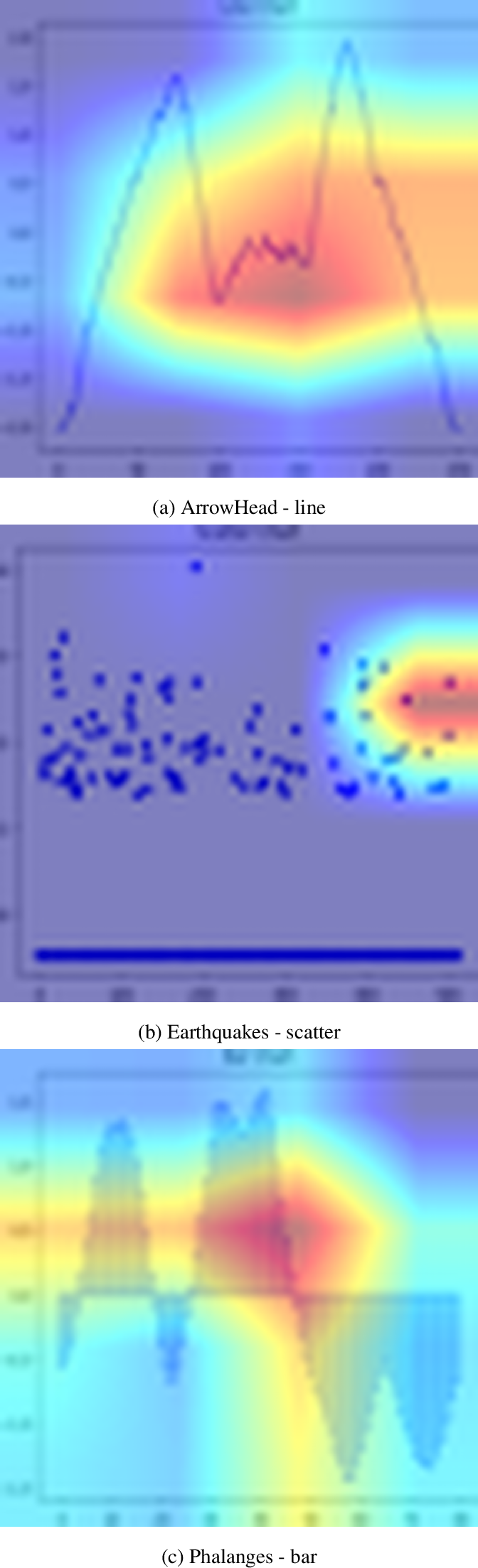
To examine model attention, we apply Gradient-weighted Class Activation Mapping (Grad-CAM) [7] to the final convolutional layer of each trained CNN (Fig. 2). Grad-CAM produces class-specific saliency maps, allowing us to distinguish whether models rely on (i) signal structure (e.g., temporal trends), (ii) encoding-specific features (e.g., bar edges, scatter density), or (iii) irrelevant elements (e.g., axes, gridlines). We analyze 10 correctly and 10 incorrectly classified samples per class and chart type, overlaying heatmaps on input images to compare attention patterns across encoding regimes.
Chart Perturbations. To stress-test model sensitivity to rendering-dependent visual evidence, we apply controlled perturbations as diagnostic probes: Gaussian blur (line/area charts), bar merging (bar charts), and alpha fading (scatter plots). Performance degradation (\(\Delta\) accuracy) therefore flags encoding sensitivity, but does not by itself establish that the disrupted evidence is task-irrelevant.
Generalization Across Encoding Families. As a robustness check, we evaluate whether the hijacking effect persists beyond chart-style rendering, we additionally evaluate five mathematical transforms (GASF, MTF [6], RP [31], CWT [32], STFT [33]) under the same training protocol. This tests whether observed trends extend beyond chart-style representations.
3.3 HINT Attention Guidance↩︎
To test whether model attention can be redirected toward semantically meaningful temporal regions, we apply HINT-based attention guidance (Figure 1D). Before computing the alignment loss, we mask the most salient Grad-CAM regions with a white bounding box, occluding them to isolate the model’s reliance on those cues. The masked image is then passed through the model to produce a second Grad-CAM map, used as the alignment signal. The training objective combines classification and attention alignment losses: \(\mathcal{L}_{\text{total}} = \mathcal{L}_{\text{cls}} + \lambda \cdot \mathcal{L}_{\text{HINT}}\), where \(\mathcal{L}_{\text{HINT}}\) penalizes divergence between the model’s Grad-CAM map and a target attention mask derived from temporal importance annotations. Unlike prior work relying on human annotations, our approach derives supervision from model-driven saliency, enabling a self-supervised adaptation of HINT for chart-based TSC.
4 Results↩︎
4.1 Representational Divergence Across Chart Types↩︎
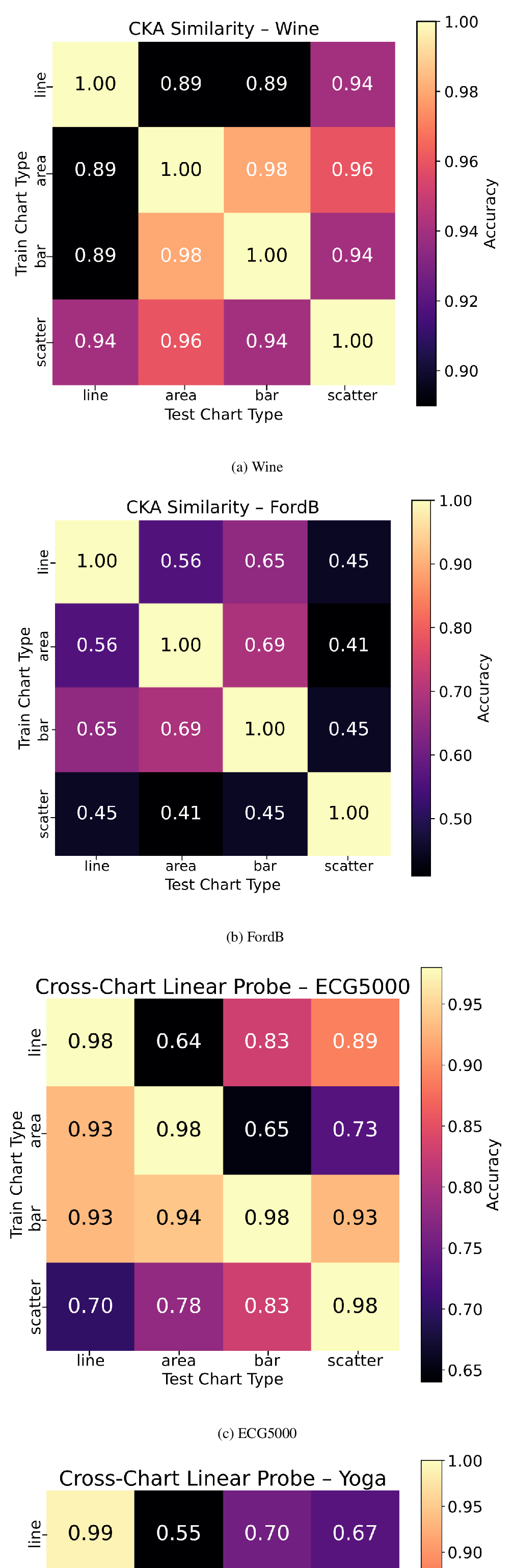
Encoding alignment is bimodal; representations from simple datasets achieve high convergence, whereas those from complex datasets show substantial divergence (RQ1, RQ2). CKA analysis reveals a relationship between dataset complexity and representational alignment across chart types. As seen in Fig. 3 (a), simple binary-class datasets (Wine) show high CKA scores (\(\approx\)0.89–0.98), indicating encoding-invariant representations. Complex, multi-class datasets like FordB (Fig. 3 (b)) exhibit minimal cross-chart similarity (\(\approx\)0.44–0.69), suggesting that chart type may fundamentally alter the learned feature space. Moderate-complexity datasets like GunPoint and Yoga fall in between, with area-bar pairs showing strong alignment (\(\approx\)0.86–0.96) while line and scatter diverge (\(\approx\)0.67–0.79). Cross-chart transferability follows this pattern (Fig. 3 (c-d)): encoding-invariant datasets like ECG5000 exhibit high off-diagonal accuracy (0.64–0.94), indicating that features learned from one chart type generalize effectively. In contrast, encoding-sensitive datasets like Yoga show a gap between diagonal (0.99–1.00) and off-diagonal (0.55–0.76) accuracy, suggesting that models may specialize in the visual patterns of their training encoding with limited transfer to unseen chart types.
Chart-type separation persists across dataset lengths; encoding shapes geometry independently of intrinsic dimensionality (RQ1).
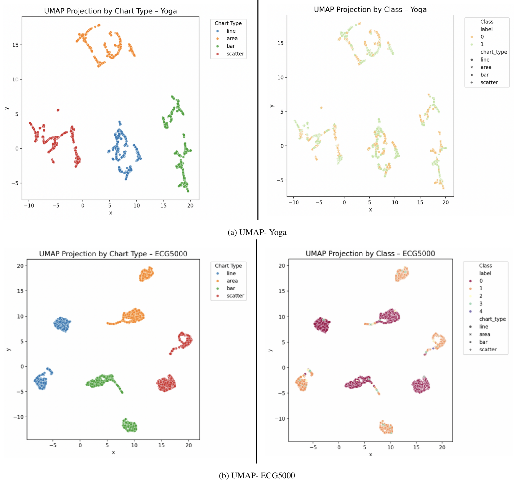
PCA and UMAP together reveal how dataset length [16] governs representational structure. Short datasets (e.g., ECG5000, GunPoint) exhibit low intrinsic dimensionality (1–11 components), and Fig. 4 (b) shows clear UMAP separation by both chart type and class. Medium datasets (e.g., Strawberry, FordB) remain low-dimensional (1–2 components) but show stronger chart-type clustering, implying increased reliance on visual encoding. Long datasets like Yoga exhibit higher dimensionality (22–26 components) with diffuse class boundaries yet clear chart-type clustering (Fig. 4 (a)), indicating that extended temporal structure expands representational capacity while amplifying encoding-specific sensitivity. Chart type minimally impacts dimensionality, confirming that dataset complexity, not visualization form, drives variance.
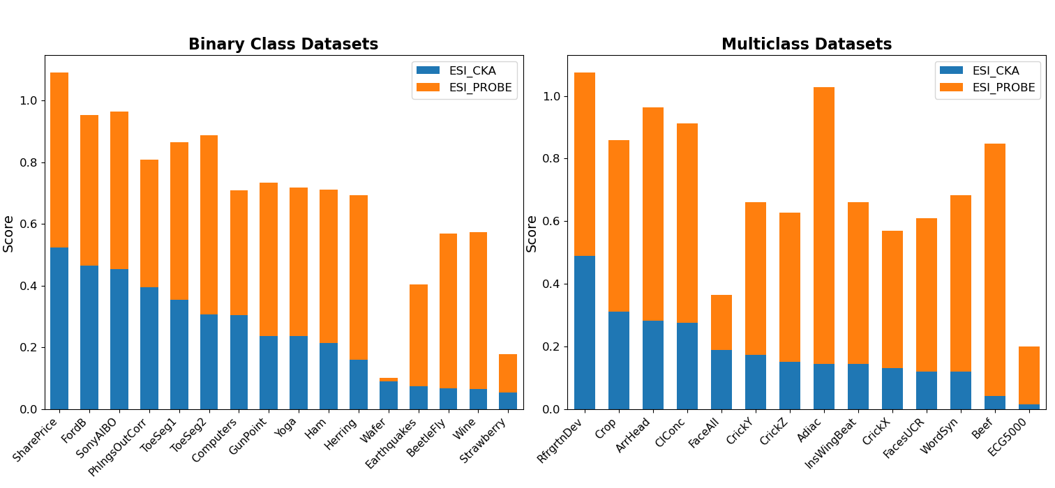
Encoding sensitivity is more strongly associated with class count than sequence length in our dataset-level analysis (RQ1, RQ2). As shown in Fig. 5, \(\text{ESI}_{\text{CKA}}\) peaks for SharePriceIncrease (0.524), FordB (0.464), and RefrigerationDevices (0.49), while \(\text{ESI}_{\text{Probe}}\) peaks for Adiac (0.883) and Beef (0.806). Cross-metric dissociations also emerge: Beef shows low representational alignment but high probe sensitivity, whereas Wafer shows relatively stable representations but weaker linear transfer. Notably, binary datasets such as Wafer and Strawberry exhibit low encoding sensitivity despite differences in sequence length, while multi-class datasets such as Adiac show elevated sensitivity even with shorter sequences [16]. These patterns suggest that class structure may be a stronger correlate of encoding sensitivity than sequence length, but further controlled analysis is needed before making a causal claim.
4.2 Model Behavior Under Controlled Perturbations↩︎
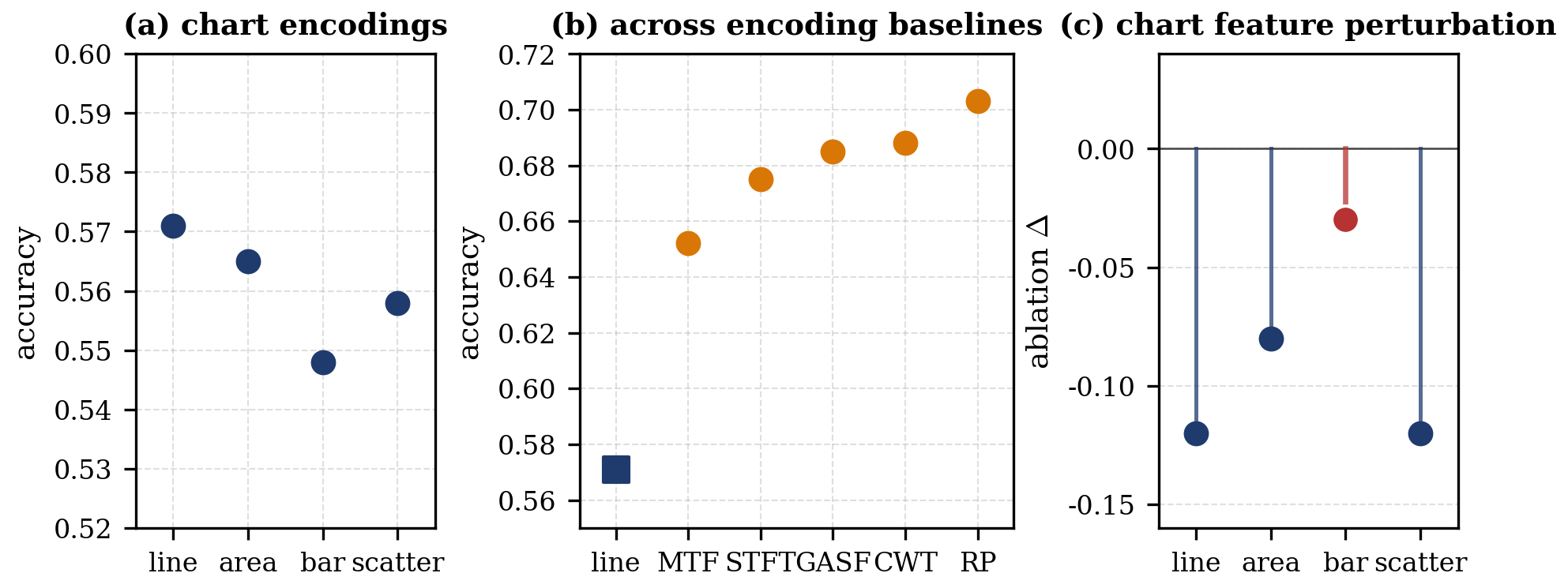
Model behavior is consistently associated with encoding-dependent inductive biases rather than encoding-invariant representations (RQ3). In VEIL, no encoding consistently dominates across datasets, suggesting that chart features act as distinct inductive priors rather than interchangeable inputs (Fig. 6a). Performance differences become more pronounced across encodings, indicating that encoding choice can substantially alter the feature distributions learned by the model (Fig. 6b). Targeted perturbations further serve as diagnostic stress tests, revealing sensitivity to rendering-dependent visual evidence: performance drops when key visual elements are disrupted, while bar charts remain comparatively robust, suggesting lower sensitivity to fine-grained features and greater reliance on coarse structural patterns (Fig. 6c). These results show sensitivity to encoding-specific visual elements, but do not establish that the disrupted evidence was task-irrelevant.
4.3 HINT Attention Guidance↩︎
| Dataset | Best Encoding | Baseline (%) | HINT (%) | Delta (%) | |
|---|---|---|---|---|---|
| ArrowHead | Area | 30.29 | 39.43 | +9.14 | |
| PhalangesOutlinesCorrect | Scatter | 65.15 | 61.31 | -3.85 | |
| ChlorineConcentration | Bar | 55.78 | 53.26 | -2.53 | |
| SonyAIBORobotSurface1 | Line | 57.07 | 42.93 | -14.14 | |
| Adiac | Scatter | 22.51 | 39.13 | +16.62 | |
| FaceAll | Scatter | 77.93 | 75.92 | -2.01 | |
| FacesUCR | Area | 57.12 | 77.66 | +20.54 | |
| CricketX | Scatter | 52.56 | 63.59 | +11.03 | |
| CricketY | Scatter | 55.38 | 64.10 | +8.72 | |
| CricketZ | Area | 54.36 | 65.38 | +11.03 | |
| ToeSegmentation1 | Scatter | 47.37 | 55.70 | +8.33 | |
| ToeSegmentation2 | Area | 43.08 | 81.54 | +38.46 | |
| Wine | Bar | 50.00 | 50.00 | 0.00 | |
| InsectWingbeat | Area | 57.24 | 63.68 | +6.34 | |
| WordSynonyms | Scatter | 48.75 | 53.76 | +5.02 | |
| Beef | Scatter | 20.00 | 20.00 | 0.00 | |
| BeetleFly | Scatter | 50.00 | 50.00 | 0.00 | |
| Computers | Bar | 69.60 | 33.60 | -36.00 | |
| Earthquakes | Scatter | 69.06 | 74.82 | +5.76 | |
| Ham | Area | 50.48 | 74.29 | +23.81 | |
| Herring | Area | 40.62 | 59.38 | +18.75 | |
| RefrigerationDevices | Area | 54.13 | 53.87 | -0.27 | |
| SharePriceIncrease | Line | 58.59 | 68.63 | +10.04 | |
| Crop | Bar | 47.68 | 68.60 | +20.92 | |
| ECG5000 | Line | 93.44 | 93.29 | -0.16 | |
| GunPoint | Area | 49.33 | 61.33 | +12.00 | |
| Strawberry | Bar | 90.00 | 93.78 | +3.78 | |
| FordB | Bar | 62.96 | 73.58 | +10.62 | |
| Wafer | Area | 99.50 | 99.59 | +0.10 | |
| Yoga | Line | 49.80 | 52.60 | +2.80 | |
| Lightning2 | Area | 54.10 | 54.10 | 0.00 |
HINT improves performance on several encoding-divergent datasets but is not a general mitigation strategy (RQ3). As shown in Table 1, HINT gains align with prior diagnostics. Encoding-divergent datasets (low CKA, low cross-chart transfer, high \(\text{ESI}_{\text{Probe}}\) \(> 0.5\), UMAP clustering by chart type) show substantial improvements: ToeSegmentation2 (+38.46%), Ham (+23.81%), Crop (+20.92%), and FacesUCR (+20.54%). Encoding-invariant datasets (high CKA, strong transfer, low \(\text{ESI}_{\text{Probe}}\) \(< 0.2\), UMAP mixing by class) show minimal effects (ECG5000: -0.16%, Wafer: +0.10%). PCA confirms that dimensionality alone does not predict HINT effectiveness. Area and scatter encodings benefited most, consistent with UMAP evidence of distinct clustering. However, HINT degraded performance for Computers (-36.00%), SonyAIBORobotSurface1 (-14.14%), and PhalangesOutlinesCorrect (-3.85%), suggesting that attention guidance may interfere with already-effective representations. These results suggest that attention guidance can reduce encoding-sensitive behavior in selected cases when supported by convergent evidence across CKA, linear probe, ESI, UMAP, and PCA, but its failures indicate that HINT should be treated as a diagnostic intervention rather than a reliable mitigation method.
5 Discussion and Conclusion↩︎
Our results suggest a fundamental tension in image-based TSC: models appear to learn both temporal structure and encoding-specific visual cues. We term this visual encoding hijacking, associated with cases where performance may depend on how a signal is rendered, not what it represents. (1) Encoding as inductive bias: visual encoding appears to be a potential source of inductive bias, as chart types produce divergent feature spaces and inconsistent transfer, so encoding choice may warrant the same care as model design. (2) Rethinking performance gains: high accuracy does not necessarily imply semantic understanding, since models may exploit encoding-specific artifacts, raising concerns about cross-encoding comparisons. (3) Toward diagnostic evaluation: accuracy alone is insufficient; combining similarity, transferability, attribution, and perturbation stress tests reveals encoding sensitivity. Perturbations do not prove that encoding-dependent evidence is task-irrelevant. Overall, VEIL addresses a growing question: how do vision models perceive charts? While graphical perception studies human interpretation of visualizations, VEIL examines model interpretation, showing that visual encoding choices shape learned representations, though these effects do not always reflect semantic understanding. Encoding choice substantially affects what models learn, making chart design consequential for both human communication and machine consumption. These findings motivate encoding-aware evaluation protocols that better align model reasoning with human-interpretable structure.
References↩︎
Emails: {ssooraj, lanche, mvenkat, dyuliu}ucdavis.edu?↩︎
Visual Encoding Illusion in Learning.↩︎