To Retain or to Adapt? Generalizing Continual Learning
July 06, 2026
Abstract
The Continual Learning (CL) literature has long been driven by the goal of mitigating catastrophic forgetting. This objective rests on a pervasive, often unstated assumption: that a lifelong learner should approximate the Joint-Task Learning (JTL) solution and retain all previously acquired knowledge. We challenge this retention-centered premise, arguing that in non-stationary environments prioritizing retention can impede real-time adaptation. Shifting the focus to the Average Lifelong Error (ALE), we formalize CL as an online optimization problem governed by the interaction between environmental and learning dynamics. We introduce Transfer Efficiency as a quantitative measure of the tension between Instability, the bias inherited from conflicting past experience, and Transient Error, the optimization cost of learning new tasks from scratch. Under mild convergence conditions, holding across linear and neural network models, this decomposition yields a Critical Task Duration: a closed-form threshold beyond which historical knowledge transitions from a warm-start advantage to an optimization liability whenever retention induces a positive stationary bias. We validate these theoretical predictions on continual image classification and reinforcement learning benchmarks. Finally, by connecting continual learning to the online learning framework of predictable sequences, we show that JTL is only one instance of a broader family of objectives, and we propose a new general class of continual learning algorithms, which we call Predictive Continual Learning. Predictive CL algorithms optimize expected future performance under an explicit, dynamically updated model of future tasks. As a proof of concept, we analyze a Window algorithm that interpolates between JTL and Independent-Task Learning (ITL), outperforming both under controlled distributional drift.
0.0.1 Introduction↩︎
Real-world environments are inherently nonstationary, evolving over time and requiring systems that can adapt continually and do so efficiently. Continual learning (CL) [1]–[4]—also known as lifelong learning—addresses this challenge by developing algorithms that can acquire, retain, and update knowledge over extended sequences of experience. Unlike conventional machine learning, where the data distribution is fixed, continual learning operates under distributional drift, where performance must be maintained relative to a moving target.
Progress in continual learning has historically been guided and measured by a diverse list of metrics, which reflect the many desiderata of an adaptive agent, namely: forward transfer, minimal forgetting, preservation of plasticity, and computational efficiency [4]–[6]. This distinction of separate metrics has inevitably led to the development of methods focused only on one or a subset of those, at the expense of the other desiderata [7], [8]. Recently, [9] formally proved that maximizing real-time performance naturally leads to a trade-off between these requirements—one that is driven dynamically by the environment rather than fixed a priori. Their proposed Average Lifelong Error (ALE) objective expresses continual learning as the minimization of the online expected error in a dynamic environment, subject to resource constraints. Importantly, this perspective frames forgetting as a functional necessity to adapt within finite computations. As [9] shows, a learner with limited compute must selectively retain only the information predictive of the future, and systematically discard the rest to maintain adaptive capacity.
In the real world, it is difficult to know in advance which piece of past information will be useful in the future. Consequently, any lifelong learning algorithm must rely on assumptions or an explicit model about the future. We argue that algorithms designed to preserve performance on all previously encountered tasks, including most continual learning methods aimed at minimizing catastrophic forgetting, implicitly encode such a model. Specifically, the Joint-Task Learning (JTL) objective—the average loss over all tasks observed up to the current time— corresponds to a particular assumption about future structure: the future tasks are drawn from the same distribution as past tasks. Equivalently, JTL is the special case of ALE objective under an ergodic environment, where there statistical properties of the task stream remain stationary over time.
While this assumption can be reasonable in many scenarios, e.g. when the agent gradually explores a larger but fundamentally stable world, it breaks down when the environment changes irreversibly and past data become progressively less predictive. In such settings, optimizing the JTL objective can place excessive weight on outdated information, hindering adaptation and yielding suboptimal lifelong performance.
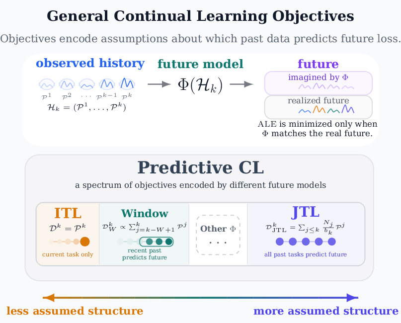
To make this perspective concrete, we contrast the JTL formulation with the Independent-Task Learning (ITL) objective, which optimizes only on the current task and retain no information from past tasks. This comparison highlights that neither objective is universally optimal. In rapidly changing environments, the ITL objective can achieve lower lifelong error by avoiding the implicit bias toward past distributions. Conversely, when past experience remains predictive of the future, the JTL objective benefits from this bias to accelerate learning and improve generalization. By analyzing these two extremes in both controlled quadratic models and deep neural networks, we characterize the conditions under which memory becomes a liability for learning. This analysis introduces three key concepts: Transfer Efficiency, which quantifies this trade-off; Instability, which measures the cost of bias inherited from previous tasks; and Transient Error, which captures the cost of learning a new task from scratch.
Our framework connects several adjacent literatures—online learning, multi-task learning, and learning to learn— revealing a shared theoretical foundation. It offers analytical tools to challenge and extend existing theories. In particular, the connection to the online learning literature allows us to interpret the JTL and ITL objectives as part of a family of algorithms based on the concept of predictable sequences [10]. In light of this connection, we propose a generalization of continual learning algorithms beyond the restrictive assumption of ergodicity. Rather than optimizing for perfect retention or complete adaptation, the objective becomes minimizing the expected future error under a model of future tasks, where the predictive model itself may be learned and updated online. We refer to algorithms that optimize this generalized objective as Predictive Continual Learning (Predictive CL). This formulation transforms the space between JTL and ITL from a gap between two extremes into a principled design space, enabling continual learning algorithms to adapt their retention strategy to the structure of the environment rather than to a fixed, a priori objective.
0.0.1.0.0.1 Contributions.
We summarize the main contributions of this paper as follows:
We recast continual learning as an online optimization problem centered on Average Lifelong Error (ALE), showing that the widely adopted Joint-Task Learning (JTL) objective is not a universally optimal target in non-stationary environments, but rather corresponds to a particular assumption about future task structure.
We formalize CL as the interaction between environment dynamics and learning dynamics, revealing that the utility of memory depends jointly on task distributions, optimization dynamics, and model properties.
We introduce three analytical quantities: Transfer Efficiency, Instability, and Transient Error that decompose the benefit of transferring past knowledge. This decomposition yields a Critical Task Duration under which retained knowledge transitions from accelerating learning to hindering adaptation.
We derive closed-form expressions for these quantities in quadratic objectives, showing that the environment Growth Rate determines the asymptotic benefits of long term memory. We further demonstrate that the same mechanisms emerge empirically in deep linear models, continual image classification, and reinforcement learning benchmarks.
We connect continual learning to the online learning literature, unifying JTL and ITL within a broader family of objectives. Building on this perspective, we propose Predictive CL, a generalized framework in which algorithms optimize expected future performance under an explicit predictive model of future tasks. As a proof of concept, we analyze a Window algorithm that interpolates between ITL and JTL and outperforms both under controlled distributional drift.
0.0.2 Background & Setup↩︎
0.0.2.1 A General Objective for Continual Learning
We begin by recalling the continual learning objective introduced by [9], and instantiate it in the supervised learning setting.3 We review the main concepts here and provide an in-depth exposition in the supplementary material (1.0.1.1).
0.0.2.1.0.1 General setting.
During its lifetime, an agent accumulates a history \(H_T = \{(a_0, o_1), \dots, (a_{T-1}, o_T)\}\) of action-observation pairs in \(A \times O\). At each time step \(n\) the agent samples an action \(a_n \sim \pi_n(\cdot \mid H_n)\) from a policy \(\pi_n\) conditioned on the history. The environment then produces a new observation \(o_{n+1} \sim \mathcal{P}(\cdot \mid H_n, a_n)\), and the learner uses the new experience \((a_n, o_{n+1})\) together with the pre-existing history \(H_n\) to produce a new policy estimate \(\pi_{n+1}\).
In this work we model the learning step as a stochastic process guided by an algorithm \(\mathcal{A}\), which updates the policy according to \(\pi_n \sim \mathcal{A}(\cdot | H_n)\). Therefore, at each time step there are two interacting stochastic processes (depicted in 2): the learning process, by which \(\pi_{n}\) and then \(a_n\) are sampled, and the environment process, by which \(o_{n+1}\) is sampled. Together, these coupled processes determine the agent’s lifetime trajectory.
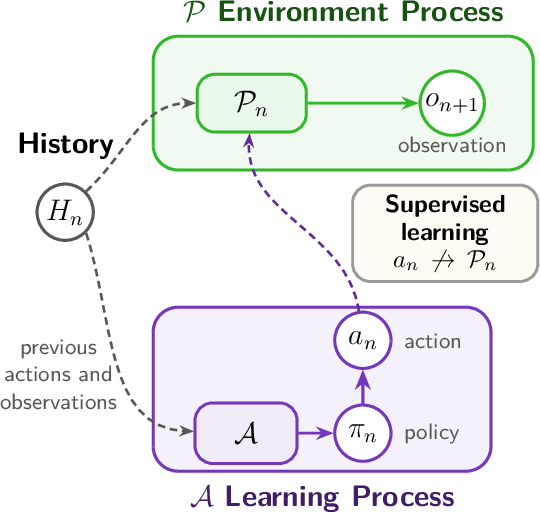
The supervised learning problem is a special case of this general formulation in which the environment process is independent of the learning process—though the converse does not hold, since the learner’s policy still depends on past observations. Concretely, the new observation \(o_{n+1}\) is independent of the action \(a_n\), so \(o_{n+1} \sim \mathcal{P}(\cdot \mid H_n)\).
0.0.2.1.0.2 Continual learning objective.
Let \(\ell(\pi, o)\) be a non-negative measure of error for a learner policy \(\pi\) when given an observation \(o\)4 and denote by \(\mathcal{P}_n\) the conditional distribution \(\mathcal{P}(\cdot |H_n, a_n)\). Lower values of \(\ell\) correspond to better performance, a convention we keep throughout the paper.
[9] define the general continual learning objective as the minimization of the real-time error: \[\begin{align} \label{eq:SLO} &\inf_\mathcal{A}\,\, \underbrace{\frac{1}{T} \sum_{n=1}^T \mathbb{E}_{\pi_n\sim\mathcal{A}(\cdot\mid H_{n}), \,o_{n+1}\sim\mathcal{P}_n}\, \left[\ell(\pi_n,o_{n+1})\right]}_{\mathrm{ALE}(\mathcal{A})} \qquad\text{s.t. computational constraints} \end{align}\tag{1}\] The computational constraints are intentionally left generic in the original formulation (Eq. 2 of [9]), as the precise formulation depends on the specific form of \(\mathcal{A}\).
Two features of this formulation are central to what follows. First, the learner is evaluated on the next-step observation \(o_{n+1}\): in stationary settings this corresponds to the conventional notion of test-error, but under non-stationarity the data distribution may change in successive time steps (\(\mathcal{P}_n \neq \mathcal{P}_{n+1}\)), causing previously acquired knowledge to lose predictive value. Second, the computational constraint on \(\mathcal{A}\) induces the essential trade-off at the heart of CL. With unlimited computational resources, an agent could retain all past information while remaining adaptive. Under realistic resource constraints, it may be better to forget past data once they cease to predict the future. As we show in the following sections, these trade-offs emerge even in simple quadratic learning problems.
0.0.2.2 Analysis Setup and Formalism
The general formulation above accommodates arbitrary forms of non-stationarity. Following the CL literature, we introduce a task-based abstraction, where the data-generating process (described by \(\mathcal{P}_n\)) is locally stationary.
Definition 1 (Task-based data generating process.). A given history \(H_T\) is a task-based sequence if the sampling distribution \(\mathcal{P}_n\) is locally stationary. The timeline is partitioned into time intervals called tasks \(S_k = [a_k,b_k]\) such that at each time step \(n \in S_k\) an observation \(o_n\) is sampled from a task-specific distribution \(\mathcal{P}^k\).
Unless otherwise stated, we assume the history is a task-based sequence with known task switch points. We denote by \(z(n)\) the task identity at time \(n\) and by \(N_k = |S_k|\) the duration of task \(k\).
With a slight abuse of notation we use \(\ell(\theta, o)\) to indicate \(\ell(\pi_\theta, o)\), where \(\theta\) are the parameters of the policy \(\pi\). We denote the expected loss for task \(k\) over the model parameters \(\theta\) as \[\mathcal{L}^k(\theta) = \mathbb{E}_{o\sim \mathcal{P}^k}[\ell(\theta, o)]\] We refer to the corresponding oracle minimizer \(\theta^k_\star \in \arg\min_\theta \mathcal{L}^k(\theta)\) as a task solution vector. Within this formalism, we define the Average Task Error as the real-time error accumulated during a single task: \[\mathrm{ALE}^k(\mathcal{A}) = \frac{1}{N_k} \sum_{n=a_k}^{b_k} \mathbb{E}_{\theta \sim \mathcal{A}(\cdot|H_n)}[\mathcal{L}^k(\theta)]\] It follows that the total lifelong error is a weighted sum of these task errors \(\mathrm{ALE}(\mathcal{A}) = \sum_{k=1}^{z(T)} \bar{w}_k \cdot \mathrm{ALE}^k(\mathcal{A})\), where the weight of each task \(\bar{w}_k = N_k/T\) is simply its relative presence over the agent’s lifetime.
Literature note. Defining \(c^k = \mathcal{L}^k(\theta^k_\star)\) the optimal value of the loss for task \(k\) for the chosen model class, we get the average regret of the optimization algorithm: \(\mathrm{ALE}^k(\mathcal{A}) - c^k\). The notion of regret is common in online learning [11]–[14], and measures the cumulative loss of a learner along its trajectory with respect to a given comparator.
0.0.2.3 The algorithm as a Markov Process
We treat the algorithm as a stochastic process. This is the most generic framing of an iterative learner: the rest of the theory in this paper instantiates it on SGD, but the definitions below cover any first-order stochastic-approximation method. More formally, we define \(\mathcal{A}\) to be a discrete-time stochastic process \(\{\theta_n\}_{n\ge 0}\) taking values in the parameter space, and we denote by \(Q_n\) the resulting parameter distribution at time \(n\). The evolution of the parameters is governed by a stochastic update rule \(U\). In this work we consider algorithms where, at step \(n\), the update rule depends on the current parameters \(\theta_n\) and a data batch \(\xi_n\) drawn from an algorithm-specific sampling distribution \(\mathcal{D}_n\): \[\theta_{n+1} = U(\theta_n, \xi_n), \quad \text{where } \xi_n \sim \mathcal{D}_n.\] This formula covers SGD as our running example and, by augmenting \(\theta_n\) to include auxiliary variables, momentum-based methods, Adam, and more broadly the entire family of stochastic approximation algorithms based on first-order Markov processes.
Crucially, the sampling distribution \(\mathcal{D}_n\) is distinct from the environmental distribution \(\mathcal{P}_n\). While \(\mathcal{P}_n\) dictates the incoming data stream, \(\mathcal{D}_n\) dictates the data used for optimization; for replay-based algorithms—such as the JTL algorithm presented here—\(\mathcal{D}_n\) may include data from previous tasks. Moreover, we assume the sampling strategy is consistent within task boundaries, such that \(\mathcal{D}_n = \mathcal{D}^k\) for all \(n \in S_k\).
Importantly, the computational cost of such algorithms depends on the complexity of the update function \(U\). For example, for SGD the complexity is proportional to the batch size used at each step, since that determines the number of forward and backward passes through the model.
Throughout this paper we reason about \(Q_n\) (the parameter distribution at step \(n\)) and its stationary limit \(Q_\infty\); in practice, expectations under \(Q_n\) are estimated from the empirical ensemble of training trajectories induced by multiple random seeds, and the deep-network experiments treat each trained model as a sample from \(Q_n\) at the corresponding step.
0.0.2.4 JTL and ITL processes
Within these boundaries, many different learning algorithms can be implemented through choices of \(U\) or \(\mathcal{D}_n\). Here we introduce two specific examples, that will be the paper’s object of study.
0.0.2.4.0.1 The Joint-Task Learning algorithm (\(\mathcal{A}_{\text{JTL}}\)).
The JTL agent aims to optimize the average loss over all seen tasks. This is equivalent to experience replay with an infinitely large buffer—often used in continual learning as an upper bound on performance. To maintain time-homogeneous dynamics within a task, we model the experience replay as a fixed mixture approximation. Specifically, the sampling distribution within task \(k\), \(\mathcal{D}^k_{JTL}\), is a weighted mixture of the current and all preceding task distributions: \[\mathcal{D}^k_{JTL} = \sum_{j=1}^k w_j^k\cdot \mathcal{P}^j, \qquad \text{where }w_j^k = \frac{N_j}{b_k}\,.\]
0.0.2.4.0.2 The Independent-Task Learning algorithm (\(\mathcal{A}_{\text{ITL}}\)).
The ITL agent optimizes solely based on the current data stream. Consequently, the sampling distribution is identical to the current task distribution, \[\mathcal{D}^k_{ITL} = \mathcal{P}^k\,.\] At the boundary between tasks, the ITL agent resets the parameters to a fixed initialization distribution, effectively discarding prior knowledge to avoid negative transfer and loss of plasticity [8]. A related variant warm-starts each task from the previous parameters instead of resetting; the differences are minor for our analysis, and we discuss them in 1.0.1.2.2.
0.0.2.4.0.3 Equivalent computational costs.
By construction, ITL and JTL share the same optimization compute per iteration: the cost scales linearly with the examples processed in a gradient update, \(\text{compute}(\mathcal{A}) \in \Theta(B)\) for batch size \(B\).5 This is the cost appearing in 1 . JTL may require additional memory or data-access machinery to implement replay, but those are outside the optimization budget studied here. Our experiments match this budget by design, using the same number of parameter updates and the same per-update batch budget for both agents.
We study JTL and ITL not as competing heuristics but as the two limiting cases of a single design axis: both are instances of the broader family of Predictive CL algorithms we formalize in 0.0.5 (6), each corresponding to a particular assumption about how the future relates to the past.
0.0.3 Transfer Efficiency↩︎
We wish to quantify when a JTL model is preferable to an ITL one. To this end, we define the concept of Transfer Efficiency, which is central to our analysis.
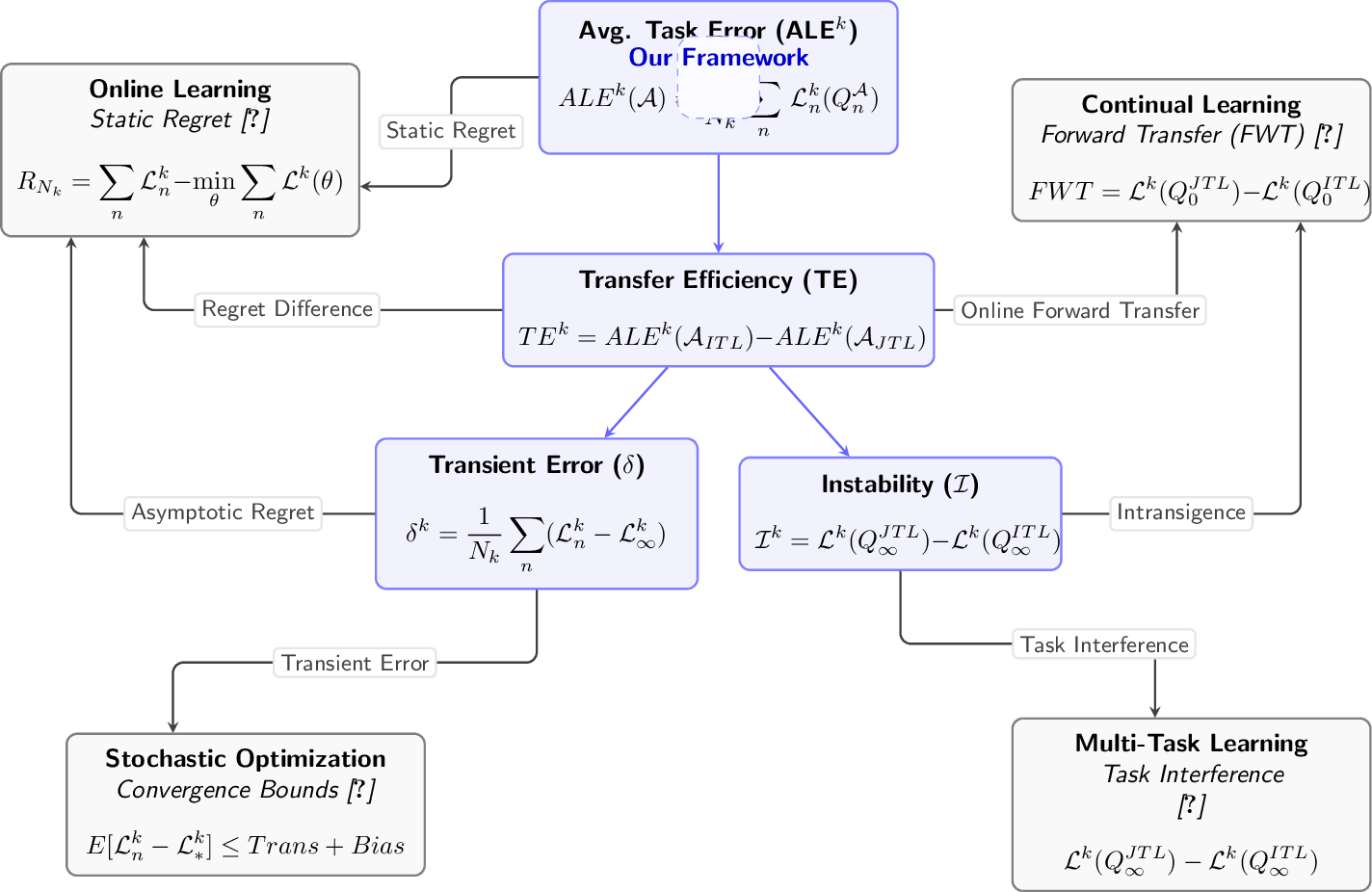
Definition 2 (Transfer Efficiency). The Transfer Efficiency for task \(k\) is the performance gain of a Joint-Task Learning (JTL) agent over an Independent-Task Learning (ITL) baseline: \[\mathrm{TE}^k := \mathrm{ALE}^k(\mathcal{A}_{\text{ITL}}) - \mathrm{ALE}^k(\mathcal{A}_{\text{JTL}}).\]
A positive value \(\mathrm{TE}^k > 0\) indicates positive transfer, where the JTL agent’s past experience improves its performance on task \(k\) relative to the ITL agent; conversely, \(\mathrm{TE}^k < 0\) indicates negative transfer. Because \(\mathrm{ALE}^k(\mathcal{A})\) represents the regret of \(\mathcal{A}\) on task \(k\) (up to a constant), the Transfer Efficiency can equivalently be read as the regret reduction obtained by JTL relative to ITL.
To understand the mechanisms of transfer, we split the error into two components: a stationary component, the error at equilibrium, and a transient component, the error accumulated while the algorithm is actively moving toward that equilibrium.6 Equilibrium is only well-defined if the optimization process converges, which we henceforth assume.
We denote by \(Q_\infty^\mathcal{A}\) the stationary parameter distribution to which \(Q_n\) converges under algorithm \(\mathcal{A}\), given a sufficiently long task duration. It is dictated jointly by the task data and the agent’s initialization at the task boundary. For the JTL and ITL algorithms we write \(Q_\infty^{JTL}\) and \(Q_\infty^{ITL}\) respectively. We also use \(\mathcal{L}^k(Q) := \mathbb{E}_{\theta \sim Q}[\mathcal{L}^k(\theta)]\) to lift the expected loss to a distribution over parameters.
Definition 3 (Instability). The Instability of a task \(k\) (\(\mathcal{I}^k\)) is the performance gap between the JTL and ITL agent measured at convergence \[\mathcal{I}^k := \mathcal{L}^k(Q_\infty^{JTL}) - \mathcal{L}^k(Q_\infty^{ITL}).\]
Definition 4 (Transient Error). The Transient Error of a task \(k\) and algorithm \(\mathcal{A}\) (\(\delta^k(\mathcal{A})\)) is the average deviation from the stationary risk over the task duration \(S_k\): \[\delta^k(\mathcal{A}) = \frac{1}{N_k}\sum_{n\in S_k} \left(\mathcal{L}^k(Q^\mathcal{A}_n) - \mathcal{L}^k(Q^\mathcal{A}_\infty)\right).\]
Combining these definitions yields a handy decomposition of Transfer Efficiency, separating the “quality of the final solution” from the “speed of learning” (visualized in 19, appendix).
Lemma 1 (TE Decomposition). For any task \(k\), assuming the algorithms converge, the Transfer Efficiency decomposes exactly as: \[\label{eq:TE-decomp} \mathrm{TE}^k = \underbrace{-\mathcal{I}^k}_{\text{Stationary Gap}} + \underbrace{(\delta^k(\mathcal{A}_{\text{ITL}}) - \delta^k(\mathcal{A}_{\text{JTL}}))}_{\text{Learning Speed Gap}}.\tag{2}\]
Literature note. The Transient Error has been extensively studied in the stochastic optimization literature [15], whereas the Instability has been the object of study of the multi-task learning and transfer-learning literature [16], [17]. These two fields have mostly developed independently, except for work in online Meta-Learning [18], [19] where both online performance and between-task transfer are considered, and where joint-task and independent-task baselines are routinely compared. To place our definitions within this rich literature, we provide a map in 3. We discuss these connections and their context in depth in 0.0.6.
0.0.3.1 The Critical Task Duration
The decomposition in 1 yields a first general result, holding under only minimal assumptions: when the stationary JTL solution is worse than the stationary ITL solution, there is a threshold task duration beyond which the initial advantage of transfer is lost.
Lemma 2 (The Critical Task Duration). Assume a sequence of \(K\) tasks of equal duration \(N\). Let \(\Delta^k(\mathcal{A}) := N \cdot \delta^k(\mathcal{A})\) denote the cumulative Transient Error of algorithm \(\mathcal{A}\) on task \(k\), let \(\bar{\Delta}(\mathcal{A}) = \frac{1}{K}\sum_{k=1}^K \Delta^k(\mathcal{A})\) be its average across tasks, and let \(\bar{\mathcal{I}}\) be the average Instability. If the cumulative Transient Error is sub-linear in \(N\), i.e.\(\Delta^k(\mathcal{A}) \in o(N)\), and \(\bar{\mathcal{I}}>0\), then there exists a critical task horizon \(N^\infty_{\max}\) beyond which transfer becomes detrimental (\(\mathrm{TE} < 0\)). The breakeven horizon is: \[N^\infty_{\max} = \frac{\bar{\Delta}(\mathcal{A}_{\text{ITL}}) - \bar{\Delta}(\mathcal{A}_{\text{JTL}})}{\bar{\mathcal{I}}}.\]
In other words, if the task duration exceeds \(N^\infty_{\max}\), the ITL agent has enough time to overcome its poor initialization, eventually outperforming the JTL agent. The Critical Task Duration is inversely proportional to the average Instability in the agent’s lifetime: the more ‘unpredictable’ the world, the narrower the window for transfer. When \(\bar{\mathcal{I}}\le 0\), the stationary JTL solution is not worse on average, and the decomposition predicts no finite horizon at which retention must become detrimental. The sub-linearity condition \(\Delta^k(\mathcal{A}) \in o(N)\) requires only that the learning algorithm converges toward its stationary risk — a mild assumption holding across standard optimization regimes, from Convex Optimization to Neural Networks (see 5).
0.0.3.2 Empirical Validation of the Framework


Figure 4: Representative continual-learning trajectories for supervised benchmarks and MT10. Top two rows: CLEAR and MD5 task trajectories, showing smooth shifts with positive JTL transfer versus sharp semantic shifts with negative transfer. Bottom row: selected MT10 per-task success-rate trajectories on Meta-World in an easy-to-hard ordering with batch size 5000 (drawer-close, window-close, reach). Both supervised benchmarks report test accuracy, while MT10 reports success rate. ITL is shown in orange, JTL in violet, and the green trace gives the JTL advantage. CLEAR shows a consistently positive advantage, while MD5 and MT10 show negative advantage after the initial transient, matching the Instability ordering..
We use three benchmarks, chosen to span a range of Instabilities: CLEAR [20], ten image classes evolving smoothly over 2004–2014; MD5, a sequence we construct from five unrelated public classification datasets with sharp semantic transitions (introduced in this paper); MT10 [21], a 10-task suite of Meta-World robotic-manipulation environments previously used to highlight continual-learning interference [7]. We use the same task duration \(N\) across tasks and tune hyperparameters for the lowest ALE per algorithm; full setup details are in 1.0.2.
Throughout the paper, classification performance is reported as accuracy in \([0,1]\) and reinforcement-learning performance as success rate in \([0,1]\). We summarize each agent by its Average Lifelong Accuracy (\(\texttt{ALA}\)) or Average Lifelong Success Rate (\(\texttt{ALS}\))—monotone (higher-is-better) re-readings of the ALE—and we sign Transfer Efficiency so that \(\mathrm{TE}>0\) always means JTL outperforms ITL.
Running ITL and JTL with matched compute on each, the resulting learning curves (4) and average lifelong performance (1) already tell the qualitative story: where Instability7 is large (MD5, MT10), joint training confers no advantage and is at times actively worse; where Instability is small (CLEAR), it confers a large, compounding advantage. In short, the sign of Transfer Efficiency tracks the sign of \(-\mathcal{I}\), exactly as 2 predicts.
| \(N\) | \(\mathbf{ALA_{ITL}}\) | \(\mathbf{ALA_{JTL}}\) | \(\mathbf{{\mathrm{TE}}}\) | |
|---|---|---|---|---|
| MD5 | 3000 | 0.470 \(\pm 0.002\) | 0.430 \(\pm 0.005\) | -0.040 \(\pm 0.005\) |
| CLEAR | 3000 | 0.465 \(\pm 0.0004\) | 0.681 \(\pm 0.0005\) | +0.216 \(\pm 0.002\) |
| \(\mathbf{ALS_{ITL}}\) | \(\mathbf{ALS_{JTL}}\) | \(\mathbf{{\mathrm{TE}}}\) | ||
| 3-4 (lr)5-5 MT10 | 500 | 0.47 \(\pm 0.47\) | 0.28 \(\pm 0.45\) | -0.19 \(\pm 0.02\) |
Beyond this qualitative pattern, the decomposition in 2 and the Critical Task Duration of 2 make two sharper, quantitative predictions about real continual-learning systems:
(P1) Instability shifts Transfer Efficiency by an amount independent of task duration; Transfer Efficiency then decays with task duration at a \(1/N\) rate. Direct prediction of 2 : \(\mathcal{I}^k\) enters as an additive constant in \(N\), while the transient gap is averaged over \(N\) steps.
(P2) For sequences with \(\bar{\mathcal{I}}>0\), increasing \(N\) drives Transfer Efficiency from positive to negative; and once \(N\) is large enough for both agents to converge, \(\mathrm{TE}\) is dominated by \(\mathcal{I}\). Direct prediction of 2: the transient gap shrinks with \(N\), leaving the stationary Instability as the residual.
Next, we test these predictions directly, using controlled benchmarks that let us vary Instability and task duration in isolation.
0.0.3.2.0.1 (P1) Controlled Instability: Permuted- and Shuffled-CIFAR.
We manipulate Instability by perturbing the input and target distribution in CIFAR-10, creating two separate benchmarks: Permuted-CIFAR (PC-16/32) shuffles input pixels within a centred patch (preserving targets, transforming only the input distribution), and Shuffled-CIFAR (SC-10/30/50) randomly re-assigns labels to a fraction of training samples (transforming only the target distribution). We expect higher Instability in Shuffled- than in Permuted-CIFAR, as label shuffling forces the same input to map to inconsistent labels across tasks. This is confirmed by our empirical measurements, collected in ¿tbl:tab:instability?.
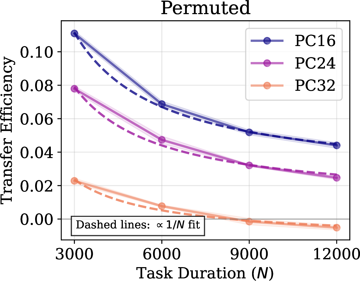
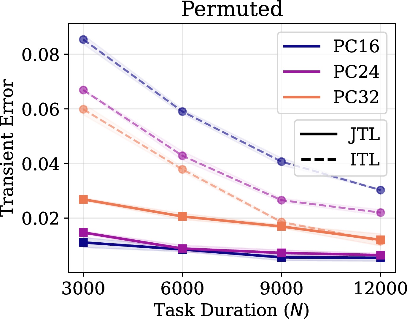
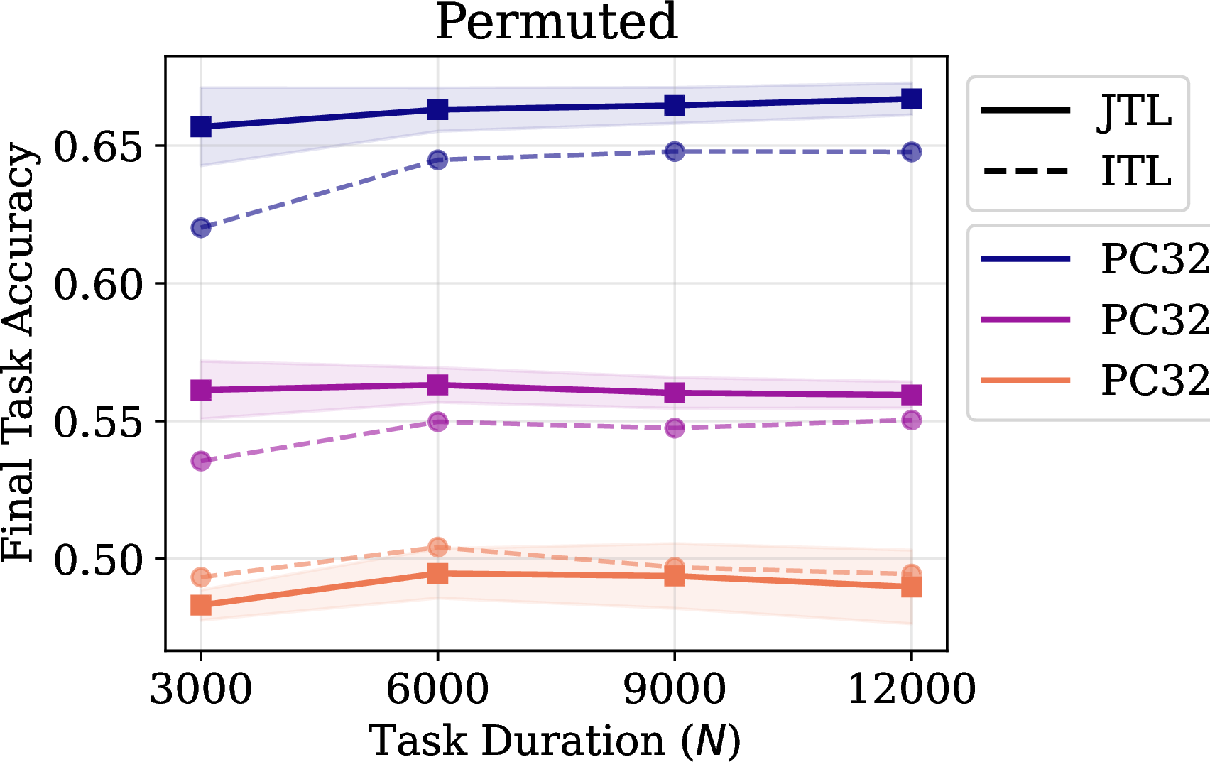
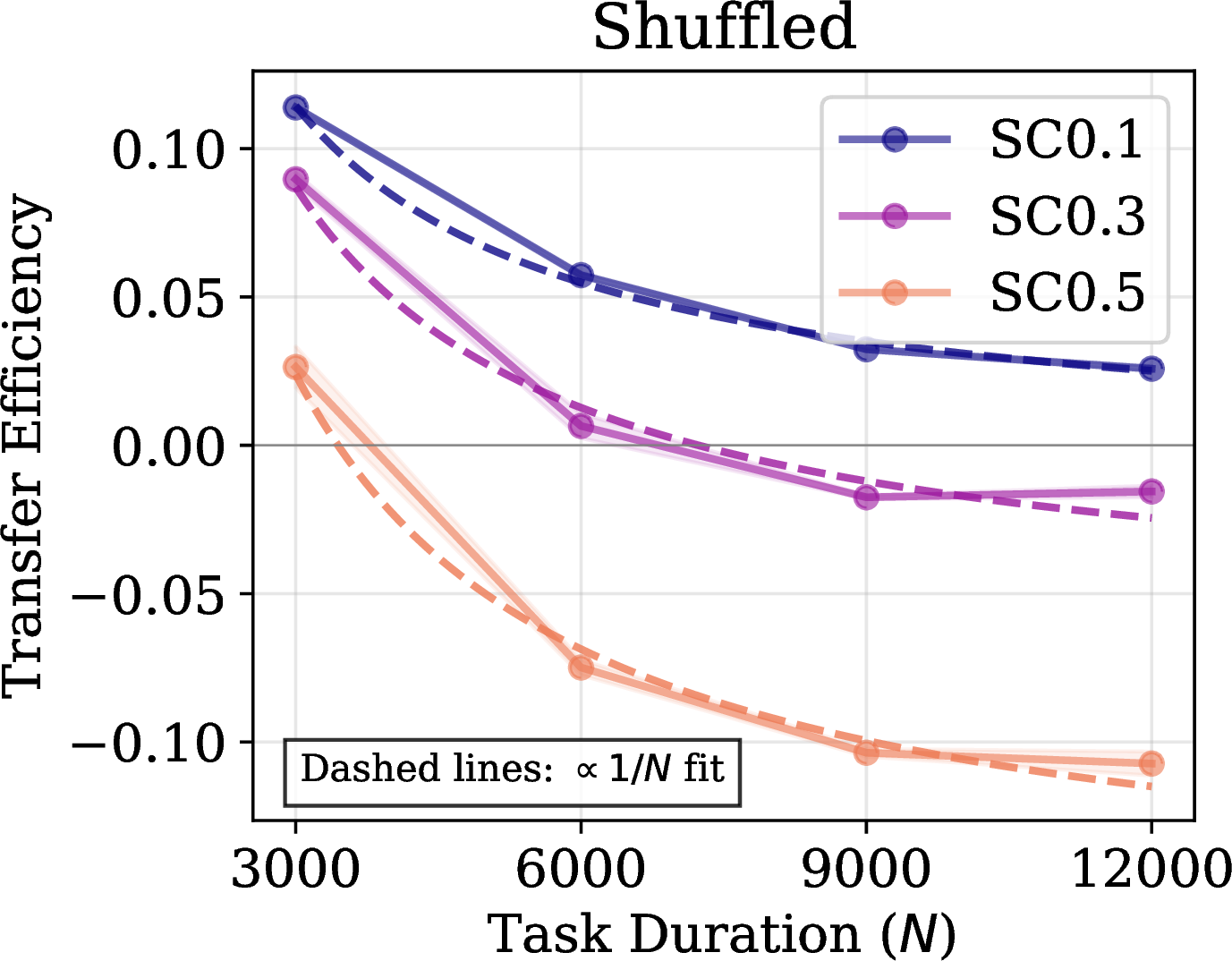
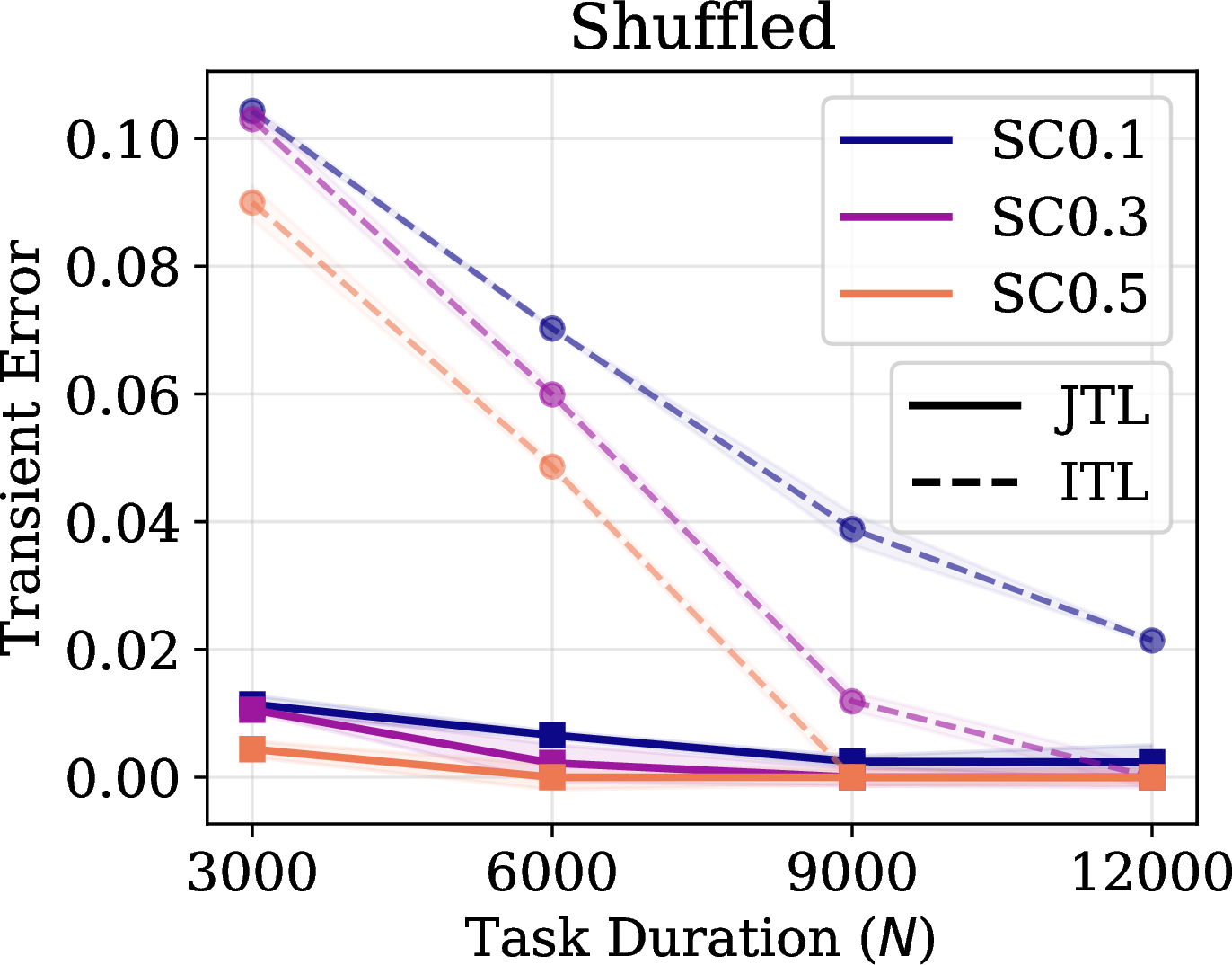
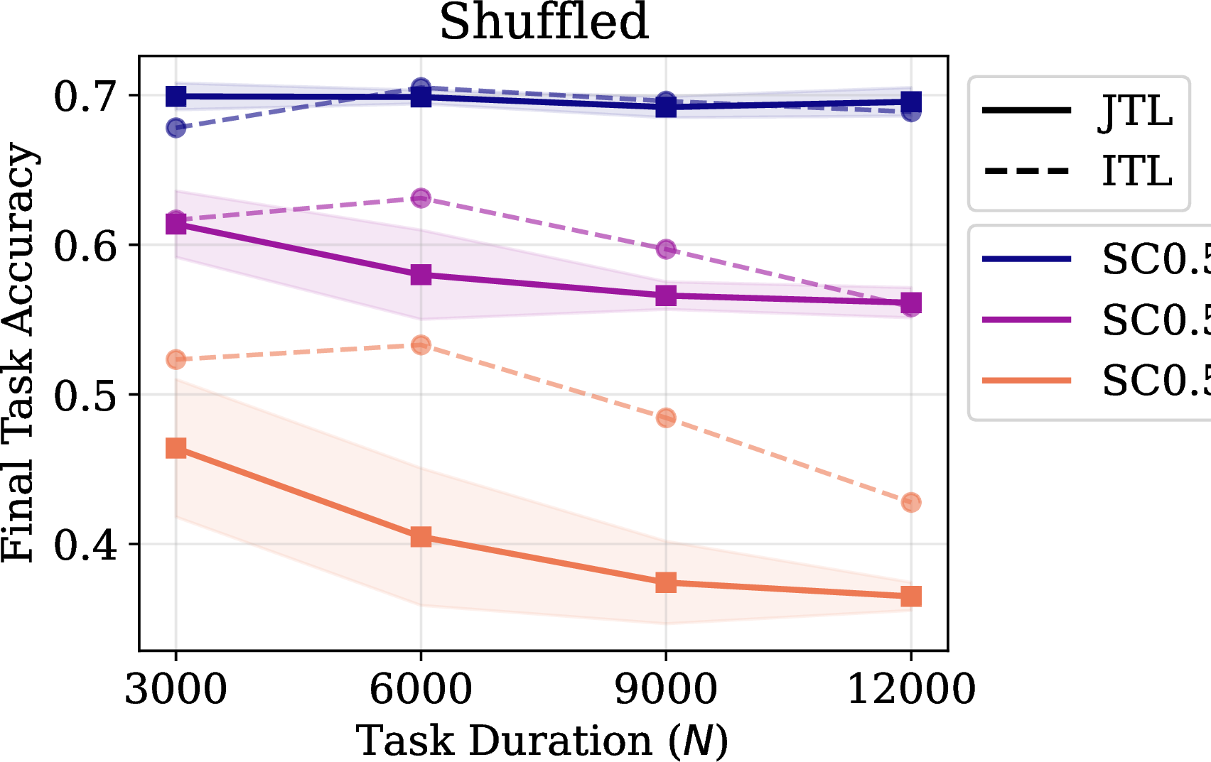
Figure 5: Manipulating Instability on CIFAR-10. Permuted-CIFAR (Top) and Shuffled-CIFAR (Bottom) across task durations \(N\). Left: Transfer Efficiency decays as \(1/N\) (dashed fits); higher Instability translates the curves vertically downward. Middle: JTL Transient (solid) is negligible relative to ITL Transient (dashed) at every \(N\), matching the asymptotic prediction. Right: Final task accuracy ceilings. To improve interpretability, all quantities are measured in accuracy (between 0 and 1)..
5 confirms each of the two halves of P1. First, increasing the shift magnitude (PC-16\(\to\)32, SC-10\(\to\)30\(\to\)50) translates the TE curves vertically downward, exactly as the additive \(-\mathcal{I}^k\) term in 2 predicts. Second, the empirical TE is well fit by a \(1/N\) curve across all settings, indicating that the per-step transient gap \(\mathcal{L}^k(Q_n) - \mathcal{L}^k(Q_\infty)\) vanishes super-linearly — the regime in which 2 applies. The middle panels additionally confirm an asymptotic prediction we revisit in 0.0.4: the JTL Transient is consistently several orders of magnitude smaller than the ITL Transient, so Transfer Efficiency is ultimately driven by Instability and the ITL Transient.
0.0.3.2.0.2 (P2) Crossing the Critical Task Duration in CLEAR.
On CLEAR where Instability is small but positive 2 predicts a finite breakeven horizon. We sweep \(N\in\{3000,6000,9000,12000\}\) training steps per task and re-measure each component of the decomposition.
| \(N\) | \(ALA_{ITL}\) | \(ALA_{JTL}\) | \({\mathrm{TE}}\) | \(\delta_{ITL}\) | \(\delta_{JTL}\) | |
|---|---|---|---|---|---|---|
| CLEAR | 3000 | 0.465 \(\pm 0.0004\) | 0.681 \(\pm 0.0005\) | 0.216 \(\pm 0.002\) | 0.227 \(\pm 0.0013\) | 0.079 \(\pm 0.0014\) |
| 6000 | 0.562 \(\pm 0.0001\) | 0.713 \(\pm 0.004\) | 0.151 \(\pm 0.004\) | 0.195 \(\pm 0.0001\) | 0.063 \(\pm 0.0001\) | |
| 9000 | 0.610 \(\pm 0.0004\) | 0.720 \(\pm 0.001\) | 0.11 \(\pm 0.001\) | 0.166 \(\pm 0.0009\) | 0.057 \(\pm 0.0010\) | |
| 12000 | 0.641 \(\pm 0.0002\) | 0.732 \(\pm 0.0006\) | 0.10 \(\pm 0.001\) | 0.148 \(\pm 0.0004\) | 0.054 \(\pm 0.0008\) |
10pt
2 confirms P2: Transfer Efficiency falls monotonically from \(+0.216\) at \(N=3000\) to \(+0.10\) at \(N=12000\), while the Instability gap (visible in the closing JTL\(-\)ITL ALE difference) is approximately unchanged. The driver is entirely the ITL Transient \(\delta_{\text{ITL}}\), which shrinks as the ITL agent gets more time to converge on each task. Extrapolating the trend places the CLEAR breakeven horizon outside the budget we could run, consistent with CLEAR’s small empirical Instability.
0.0.4 Quadratic-Loss Analysis↩︎
This section makes the transfer mechanisms analytically transparent. We do two things. First, for quadratic losses we derive exact closed-form expressions for the Instability and the Transient Error—and hence for Transfer Efficiency—that expose how each quantity depends on the design choices (step size \(\eta\), batch size \(B\), parametrization). Second, we pass to an asymptotic (large-\(k\)) analysis that collapses these expressions into a single sufficient condition for positive transfer, governed by one environment-level descriptor: the rate at which the environment expands with new tasks. Different environments yield different balances between ITL and JTL, and this descriptor predicts which one wins.
The quadratic setting has been extensively studied in both the stochastic optimization and multi-task learning literatures, allowing us to apply existing results to our specific case. Even in such a simple setting, the interplay of learning dynamics and bias yields multiple layers of complexity, which offer powerful insights into the nature of transfer. The decomposition in 1 2 is general under task-wise convergence; the closed-form expressions below additionally use standard assumptions detailed in 1.0.1.2 (aligned positive-definite Hessians, small constant step sizes, locally stationary gradient-noise covariances, uniform observation-noise floors). These assumptions are not needed for the definitions themselves, but they make the transfer mechanisms analytically transparent.
0.0.4.1 Setup
For every task \(j \in \{1, \dots, K\}\), the expected loss is \[\mathcal{L}^j(\theta) = \tfrac{1}{2}(\theta - \theta_\star^j)^\top H_j (\theta - \theta_\star^j) + c_j,\] with \(H_j \succ 0\) (symmetric positive definite) and \(c_j\) the irreducible loss (Bayes error) for task \(j\). The Hessian \(H_j\) is data-driven: in linear regression with inputs \(x\sim\mathcal{P}^j_x\), it is simply \(H_j = \mathbb{E}_{x\sim\mathcal{P}^j_x}[xx^\top]\). The re-centered form above is convenient for the analysis, but the gradient \(\nabla\mathcal{L}^j(\theta) = H_j(\theta - \theta_\star^j) = H_j\theta - \mathbb{E}[xy]\) is computable from data without knowing \(\theta_\star^j\); we use the \((\theta_\star^j, c_j)\) parametrization only to expose the dependence of dynamics on the task minimizer.
In this setting, the expected risk for task \(k\), \(\mathbb{E}_\theta[\mathcal{L}^k(\theta_n)]\), is completely determined by the first two moments of the parameter distribution \(Q_n\): the mean \(\mu_n\) and covariance \(\Sigma_n\). Under the gradient-noise assumptions in 1.0.1.2, the stationary covariance \(\Sigma_\infty\) admits a clean decomposition into a transient part and a stationary noise part whose trace scales as \(1/B\) in the batch size.
0.0.4.2 Closed-form Instability and Transient Error
To express the Instability and Transient Error in closed form, we introduce the relative curvature matrix \(\mathcal{R}^k = H_{\text{dyn},k}^{-1} H_k\): the curvature of the current task measured against the curvature of the optimization objective (which governs the parameter dynamics). For ITL, \(\mathcal{R}^k = I\) is simply the identity. For JTL it generally is not, and the misalignment between dynamics and evaluation is precisely what makes transfer non-trivial.
Throughout this section we use the Mahalanobis-style notation \(\|v\|_M^2 := v^\top M v\) for any positive-(semi)definite matrix \(M\). A central quantity is what we call the Task Diversity: the additional variance in the optimization process due to the aggregation of multiple tasks. Recalling the task weights \(w_j^k = |S_j|/b_k\) from 0.0.2.4, \[\mathcal{V}_{div}^k = \sum_{j=1}^k w_j^k\cdot \left\|\nabla\mathcal{L}^j(\theta_\star^{JTL,k})\right\|_{\mathcal{R}^k}^2,\] where \(\theta_\star^{JTL,k}\) is the minimizer of the JTL objective at task \(k\). The norm is taken in the relative-curvature geometry, so tasks whose gradients are large along directions the optimizer treats as informative contribute more.
Within these assumptions, the Instability of task \(k\) admits an exact decomposition into a bias term and a variance term proportional to the Task Diversity (full derivation in 2): \[\mathcal{I}^k = \underbrace{\mathcal{L}^k(\theta_\star^{\text{JTL},k}) - \mathcal{L}^k(\theta_\star^{k})}_\text{JTL Bias} + \,\underbrace{\,\,\frac{\eta}{4\,B}\,\mathcal{V}_{div}^k\,\,}_\text{JTL Variance}.\] The two terms describe distinct cost sources of joint training. The JTL Bias is the structural penalty: the JTL solution \(\theta_\star^{\text{JTL},k}\) is a compromise across the task collection, so when evaluated on a single task it pays a fixed gap relative to that task’s own optimum. The JTL Variance is the dynamical penalty: aggregating tasks injects gradient noise proportional to the step size \(\eta\) and inversely to the batch size \(B\). This noise is amplifies only along directions that the relative-curvature geometry identifies as informative—namely, directions where task \(k\)’s curvature is large relative to the pooled objective, corresponding to features that are important for task \(k\) but receive little support from the aggregated gradient of the other tasks.
The Transient Error admits an analogous decomposition (3), expressed in terms of the deviations \(\tilde{\mu}_n := \mu_n - \mu_\infty\) and \(\tilde{\Sigma}_n := \Sigma_n - \Sigma_\infty\) of the mean and covariance from their stationary values: \[\tau\,\delta^k = \frac{1}{N_k}\,\underbrace{\left(\|\tilde{\mu}_0\|^2_{\mathcal{R}^k} - \|\tilde{\mu}_{N_k}\|^2_{\mathcal{R}^k}\right)}_\text{Mean Potential Difference} + \frac{1}{N_k}\,\underbrace{\left(\text{Tr}(\mathcal{R}^k \tilde{\Sigma}_0) - \text{Tr}(\mathcal{R}^k \tilde{ \Sigma}_{N_k})\right)}_\text{Variance Potential Difference},\] where \(\tau = 4\eta\) is the learning time scale. This expression gives a clean physical reading of the cost of learning a task: it is the drop in potential energy between where the agent started the task and where it ended, measured on a quadratic potential surface warped by the relative curvature \(\mathcal{R}^k\). The transient cost is therefore high precisely when initialization is far from the task’s stationary distribution, and decays as the agent drains that potential.
0.0.4.3 Asymptotic Conditions for Positive Transfer
The exact formulas above hold at every \(k\) but are opaque. To expose how transfer depends on the environment, we now take an asymptotic (large-\(k\)) view, in which the entire ITL/JTL balance is governed by a single environment-level descriptor: the rate at which the environment expands with new tasks. Different environments yield different descriptors, and hence different balances between ITL and JTL. We call this descriptor the Growth Rate.
Definition 5 (Growth Rate). Let \(\psi: \mathbb{N} \to \mathbb{R}^+\) be a monotonically increasing function such that the expected squared distance of the \(k\)-th task from the origin scales as \[\mathbb{E}[\|\theta_\star^k\|^2] \in \Theta(\psi(k)).\]
The Growth Rate quantifies how fast the environment is expanding. If \(\psi(k) = 1\) the environment is bounded, meaning a finite diameter \(M\) contains all task-solution vectors. If \(\psi(k) = k^2\) the environment has a linear drift: tasks move with constant velocity \(\partial_k\theta_\star^k = v\). Between these extremes, a diffusive environment (\(\psi(k) = k\)) corresponds to tasks drifting via a random walk. 6 visualizes these three cases.
![Figure 6: Task Environment Growth Rates. Top Row: 2D spatial trajectories of the task optimal parameters \theta_\star^k for a single random seed over K=50 tasks. Each panel uses its own spatial scale (note the differing axis ranges, roughly \pm 1, \pm 4, and \pm 10), so that the trajectory remains visible despite the very different expansion rates. The dashed gray circles represent the theoretical expected distance from the origin (\sqrt{\mathbb{E}[\|\theta_\star^k\|^2]}) at milestones k \in \{5, 20, 50\}, providing a common reference within each panel. Bottom Row: The expected squared distance \mathbb{E}[\|\theta_\star^k\|^2] as a function of the task index k. Solid lines: empirical expectation over 500 trajectories (\pm 1 standard deviation). Dashed black lines: theoretical growth rates.](/article/2607.05609/_pdflatex/ruzvlehk.png "fig:")
We can characterize the rate at which each component of the Transfer Efficiency scales, as a function of the Growth Rate. Putting everything together we write a sufficient asymptotic condition for positive transfer:
Theorem 1 (Asymptotic behaviour of Transfer for Quadratic Objectives — Informal). In the setup described above, in an environment with Growth Rate \(\Theta(\psi(k))\) we have \[\mathcal{I}^k \in \Theta(\psi(k)), \quad \delta^k_{ITL} \in \Theta\left(\tfrac{\psi(k)}{N_k}\right), \quad \delta^k_{JTL} \in \Theta\left(\tfrac{\psi(k)}{k^2} + \psi'(k)\right),\] where \(\psi'(k)\) denotes the environment acceleration. Consequently, for environments with polynomial growth rates the expected Transfer Efficiency is positive for large \(k\) if \[\mathcal{I}^k < C^k_{ITL}\,\frac{\mathbb{E}[\|\tilde{\mu}_0^{ITL,k}\|^2]}{N_k},\] where \(C^k_{ITL}\) is a constant of the bound.
An extended version of this result and its proof can be found in 1.0.1.5.
The three rates have a clear interpretation. The Instability inherits the full \(\psi(k)\) scaling: a faster-expanding environment makes the JTL stationary compromise progressively worse on each new task. The ITL Transient is the full \(\psi(k)\) paid back through \(N_k\) steps: when each task is long, the comparative cost of restarting learning from scratch is low. The JTL Transient, by contrast, is dominated by the much smaller terms \(\psi(k)/k^2\) and \(\psi'(k)\): as \(k\) grows, the JTL agent only has to track how the environment is moving, not where it currently is, which is comparatively cheap.
For polynomial growth, Transfer Efficiency is therefore asymptotically dominated by two competing terms: the Instability \(\mathcal{I}^k\) (the JTL stationary-bias penalty) and the ITL Transient \(\delta^k_{ITL}\) (the ITL reset penalty); the JTL Transient is lower-order in the regimes we analyze. The sufficient condition in 1 reads exactly this trade-off: transfer is positive when the JTL stationary penalty is paid back within the budget the ITL agent needs to warm up. From this we rediscover the conventional wisdom that joint-task training is most valuable in the “few-shot” regime — where \(N_k\) is small and ITL has no time to recover from a cold start — and ceases to help when the environment is so unpredictable that the bias cost dominates.
0.0.4.4 The Continuous Drift Model
To make the asymptotic story concrete, we instantiate the framework on a diffusive regime: a Wiener-walk model where optimal parameters evolve as \(\theta_\star^k = \theta_\star^{k-1} + \Delta_k\) with \(\Delta_k \sim \mathcal{N}(0, \Sigma_\Delta)\), and drift magnitude \(\sigma_\Delta^2 := \text{Tr}(\Sigma_\Delta)\) controlling both how far the process may travel and how fast the relevance of past data decays. This regime captures real-world continuous distribution shifts such as the slow evolution of user preferences or weather variation in autonomous navigation. The full setup (Gaussian inputs with covariance \(\Sigma_x\), label noise \(\sigma_\xi^2\)) is in 1.0.1.6.
Applying the exact Instability and Transient Error formulas to this setup yields a non-asymptotic sufficient condition for positive transfer: a single inequality balancing an ITL Transient cost (which grows linearly in \(k\) but decays as \(1/N\)), a JTL Instability cost (which grows linearly in \(k\) with no compensating \(1/N\) factor), and a smaller JTL Transient cost (which decays in both \(k\) and \(N\)). The three terms mirror 1; the full expression is given in 8 .
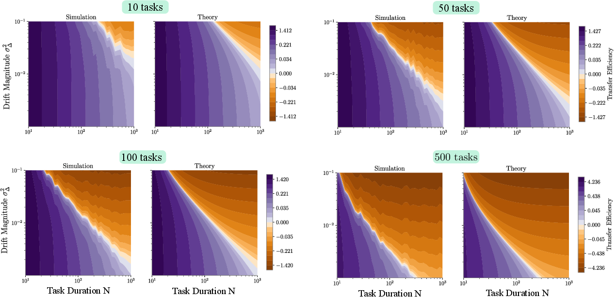
Simulations of this model (7; details in 1.0.2.1) confirm the boundary at finite \(k\) and show the positive-transfer region shrinking as \(k\) grows, since the JTL Transient is lower-order than the linear-in-\(k\) terms. In the limit \(k\to\infty\), the condition reduces to a clean closed form for the Critical Task Duration: \[\label{eq:critical-task-dur} N_{\max}^\infty = \frac{3\gamma_{\min}\,\sigma^2_\Delta}{2\eta\,\text{Tr}(\Sigma_x \Sigma_\Delta)}.\tag{3}\] This asymptotic boundary is set by the geometry of the environment together with the optimizer: it depends on the input–drift coupling \(\text{Tr}(\Sigma_x \Sigma_\Delta)\), the loss curvature \(\gamma_{\min}\), and the learning rate \(\eta\) (smaller \(\eta\) favours biased initializations such as JTL), while being invariant to the overall drift magnitude \(\sigma^2_\Delta\) and independent of the batch size \(B\). The full asymptotic landscape and a trajectory-level view of drift eroding the warm-start advantage are in 10 24.
0.0.4.5 The Optimization Bias Matters
The closed-form analysis above takes the function class as given. A complementary question is how much of the transfer profile is set by the function class versus the optimization bias of the algorithm that fits it. We isolate this by extending the Continuous Drift Model to a deep-linear teacher-student setup (following [22]; details in 1.0.2.1) and comparing two parametrizations of the same linear function class: NTP (lazy regime, [23]) and \(\mu\)P (rich regime).
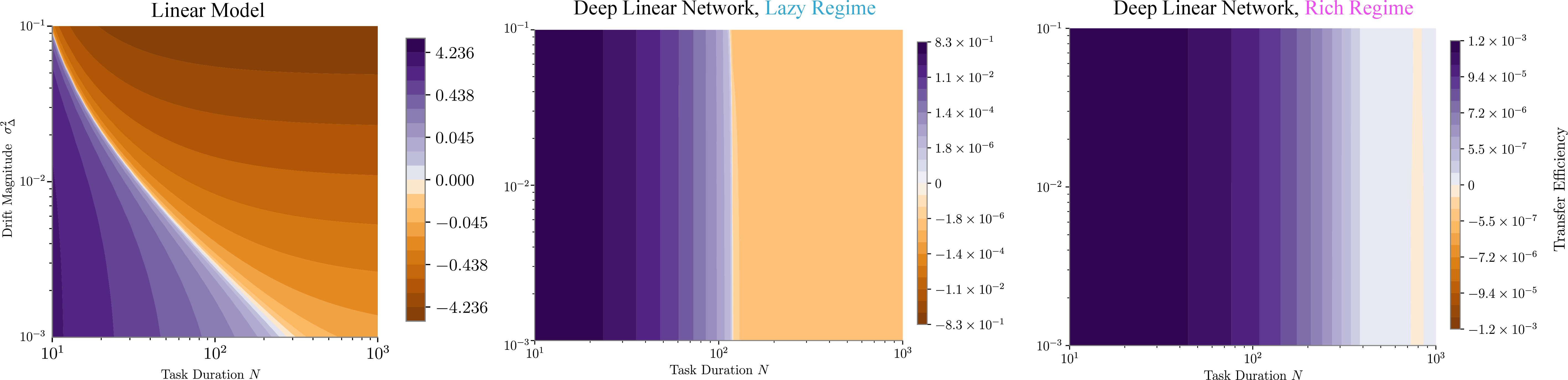
8 shows that the three TE fronts differ markedly even though the function class is the same; per-width fronts are in 21 22. Examining the constituents (23) reveals two observations consistent with 1: Instability is several orders of magnitude higher under NTP, yielding substantially lower JTL performance; and the JTL Transient is several orders of magnitude below the ITL Transient and Instability at every width. Two implications: first, the framework continues to hold: Transfer Efficiency is governed by \(-\mathcal{I}\) plus a vanishing transient gap, but the value of \(\mathcal{I}\) is determined by implementation-level choices, not by the task sequence alone. Second, this highlights the limit of any purely statistical account of transfer (cf.the early Learning-to-Learn literature): the design of adaptive algorithms must jointly consider the stochastic processes defined by the data and by the optimizer.
0.0.5 Generalizing CL beyond the JTL/ITL dichotomy↩︎
0.0.5.1 From implicit to explicit future models
We have shown, empirically and theoretically, that neither the JTL nor the ITL algorithm is universally optimal: each minimizes the Average Lifelong Error (1 ) only under specific environmental regimes. This raises the natural question: is there a single optimal objective for continual learning, one that provably minimizes the ALE?
Foundational results in online convex optimization [24] established that, when the environment is unpredictable (i.e.adversarial), no first-order stochastic method can outperform online gradient descent [13]. However, [10] tell us that much more can be hoped for when the future is somewhat predictable. If \(\mathcal{P}_{n+1}\) were known, we could choose \(\mathcal{D}_n\) to match it and minimize the next-step loss directly; \(\mathcal{P}_{n+1}\) is not known in general, but one can always approximate the future based on some assumptions.
This lets us reinterpret the sampling choice (the choice of \(\mathcal{D}_n\)), and more generally the choice of objective, as an implicit assumption about the future. For JTL, the assumption is that the environment is ergodic and the future will resemble the past — the classical i.i.d.premise underlying empirical risk minimization. For ITL, the assumption is the opposite: that no structure can be reliably extrapolated, in which case online gradient descent on the current task is minimax-optimal [13], [24].
Algorithms that maximize average accuracy or minimize forgetting can be viewed as implicit (or, for replay-based methods, explicit) approximations of the JTL objective. Thus the proposed re-reading opens a new way to analyze and to build CL algorithms. More importantly, the same framing suggests a constructive path: rather than fix an objective implicitly, one can make the future model an explicit design choice. We call the resulting family Predictive CL algorithms.
Definition 6 (Predictive CL Algorithm). Let \(\mathcal{H}_{<k}\) denote the observable history up to task \(k\), including past data, environments, and learning trajectories. A prediction mapping \(\Phi\) maps this history to a predicted target distribution for the current task, \(\tilde{\mathcal{P}}^k = \Phi(\mathcal{H}_{<k})\). A Predictive CL algorithm optimizes its parameters by minimizing the expected loss under the predicted distribution \(\tilde{\mathcal{P}}^k\): \[\begin{align} \label{eq:GCLA} &\inf_\mathcal{A}\,\, \frac{1}{N_k} \sum_{n=a_k}^{b_k} \mathbb{E}_{\theta_n\sim\mathcal{A}(\cdot\mid H_{n}) \,}\mathbb{E}_{o\sim\tilde{\mathcal{P}}^k}\, \left[\ell(\theta_n,o)\right]\qquad\text{s.t. computational constraints} \end{align}\tag{4}\]
6 generalizes existing CL objectives by making the future model explicit. JTL is recovered by choosing \(\Phi(\mathcal{H}_{<k}) = \sum_{j\le k} w_j^k\,\mathcal{P}^j\) (the empirical past is the prediction); ITL is recovered by \(\Phi(\mathcal{H}_{<k}) = \mathcal{P}^k\) (the current task is the prediction). The Window algorithm introduced below sits between these limits. Crucially, \(\Phi\) need not be fixed: it can itself be a learned model of the future.
0.0.5.2 Proof of Concept: the Window Predictive CL Algorithm
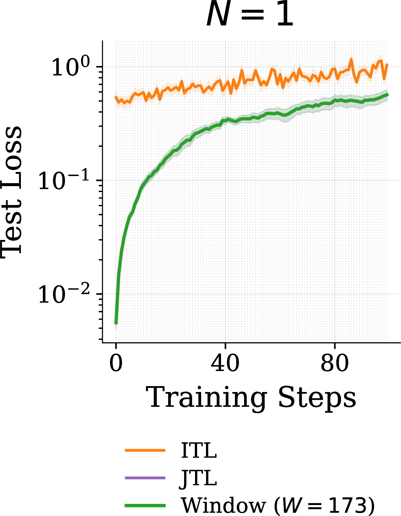
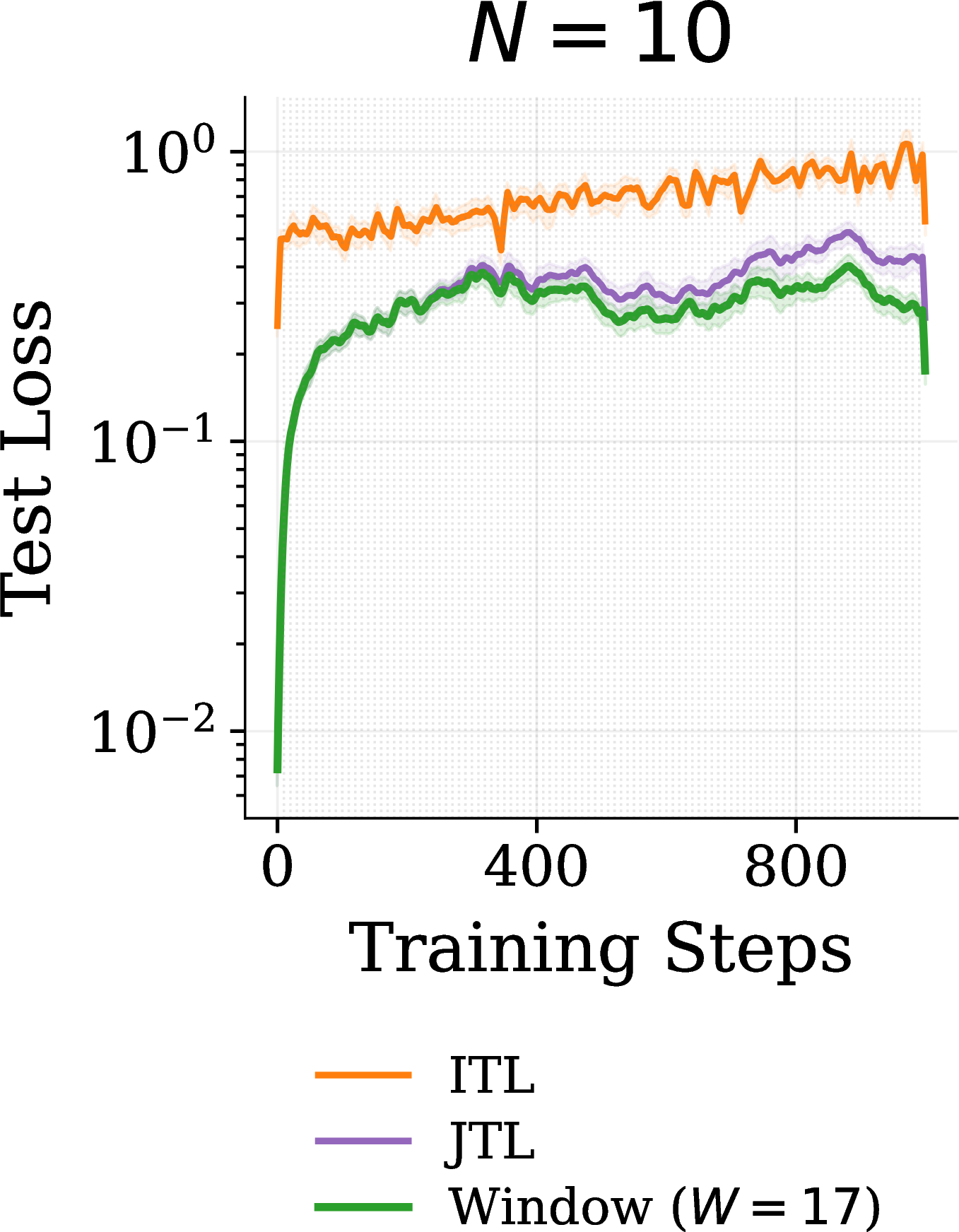
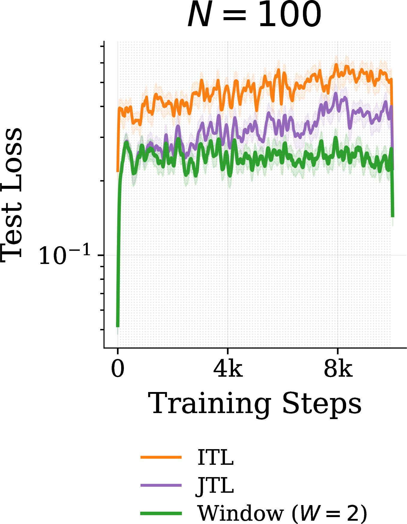
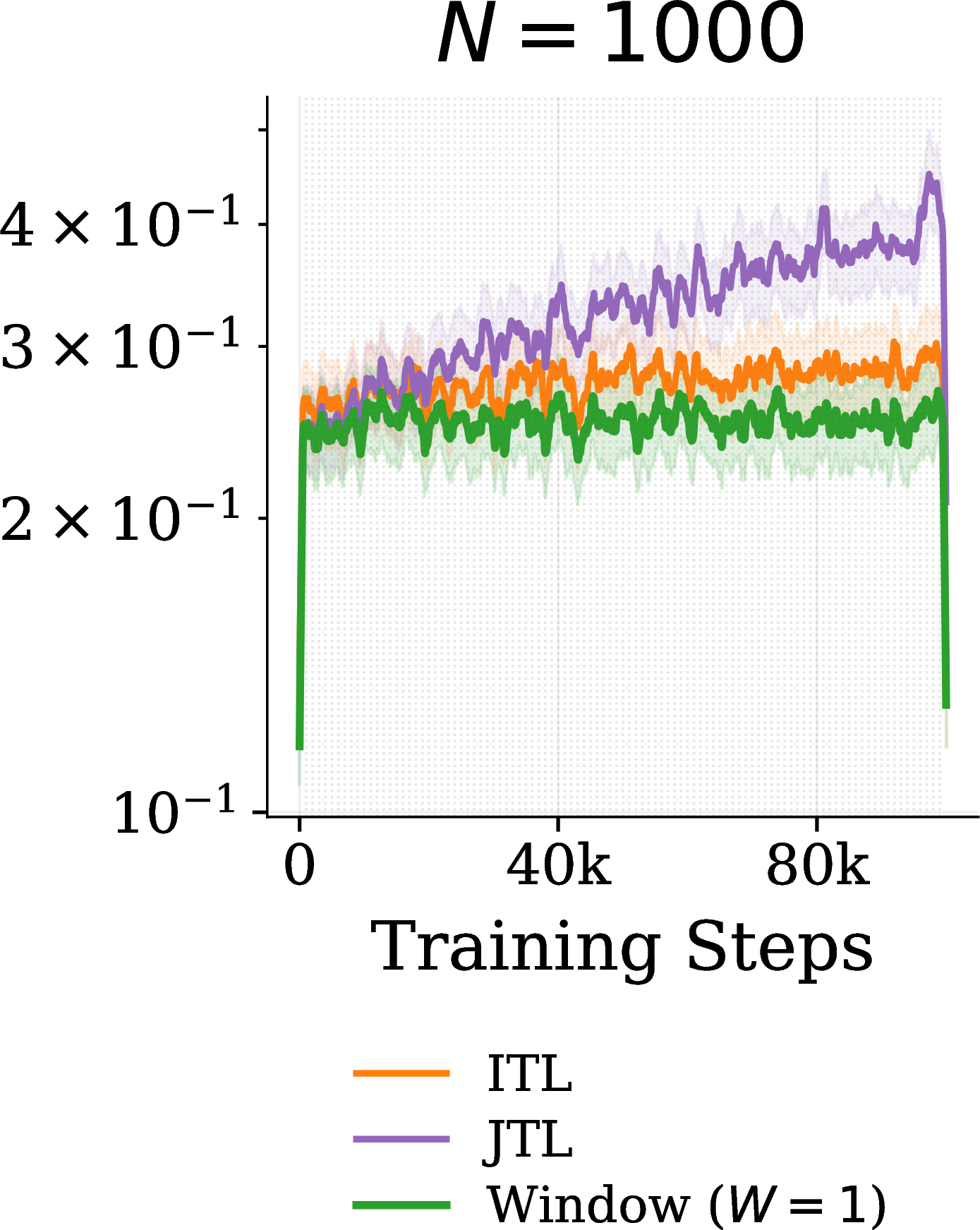
Figure 9: Real-Time Performance of the Window Algorithm. Test loss trajectories for the ITL (orange), JTL (violet), and Window (green) agents across varying task durations \(N\). The curves are smoothed by averaging over \(N\) steps. By setting the window size to the theoretical optimum \(W^\star\) derived in 11 , the Window agent consistently matches or outperforms both baselines. Notably, the optimal memory horizon is inversely proportional to task duration: shorter tasks (\(N=1\), left) call for a large memory window (\(W^\star=173\), effectively recovering JTL), whereas longer tasks (\(N=1000\), right) favor a nearly memoryless approach (\(W^\star=1\), equivalent to ITL with warm starts). The intermediate panels follow the same trend (\(W^\star=17\) at \(N=10\) and \(W^\star=2\) at \(N=100\))..
Consider again the quadratic losses case of 0.0.4. We now instantiate, as an example, a Predictive CL algorithm which we call the Window (W) algorithm. The Window algorithm predicts the future using a finite recent history: it is defined by a hyper-parameter \(W\), which we call window size. For each task \(k\) the SGD sampling distribution \(\mathcal{D}^k_W\) is a mix of the past \(W\) tasks \[\mathcal{D}^k_W = \sum_{j = k-W+1}^k w_j^k \,\mathcal{P}^j.\] Like the JTL agent, the Window agent parameters are not reset at the beginning of a new task. As \(W\) grows the window agent converges to the JTL agent - which can be seen as an infinite window agent-, whereas for \(W = 1\) it coincides with an ITL agent with warm starts.
In contrast to the JTL agent, whose bias is determined by the global growth of the task solutions relative to the origin, the Window agent’s bias depends on the local variations of the environment over the horizon \(W\). In order to capture this bias asymptotically we need to introduce a new measure, akin to the Growth Rate, which we call the Mean Squared Displacement.
Definition 7 (Mean Squared Displacement (MSD)). The Mean Squared Displacement \(m: \mathbb{N} \times \mathbb{N} \to \mathbb{R}^+\) characterizes the expected squared Euclidean distance between two task solutions separated by a lag \(W\) at time \(k\): \[\mathbb{E}[\|\theta_\star^k - \theta_\star^{k-W}\|^2] \in \Theta(m(k, W)).\]
Based on the MSD measure, we can compute the asymptotic Transfer Efficiency of the Window Algorithm compared to ITL training (as by 0.0.4.4), and we can solve for the window size \(W\) which maximises the Transfer Efficiency.
Lemma 3 (Asymptotic Optimality of Window Size). Let \(m(k,W)\) be the Mean Squared Displacement of tasks within a window \(W\). The optimal window size \(W^*\) maximizing transfer depends on the environment’s non-stationarity regime. In particular consider three examples:
Bounded Regime (\(\psi(k)=1\)): If \(m(k,W) \in \Theta(1)\), transfer increases monotonically with \(W\). The asymptotically optimal strategy is the JTL agent (\(W^* \to \infty\)).
Linear Drift Regime (\(\psi(k)=k^2\)): If \(m(k,W) \in \Theta(W^2)\), transfer decreases monotonically with \(W\). The asymptotically optimal strategy is the ITL agent (\(W^* = 1\)).
Diffusive Regime (\(\psi(k)=k\)): If \(m(k,W) \in \Theta(W)\), transfer is strictly convex in \(W\). The asymptotically optimal strategy is a Window agent with finite memory (\(1 < W^* < \infty\)).
This result formally establishes that the best objective for real-time performance depends on the environment and the model (\(m(k,W)\) is model-dependent). The bounded and linear-drift cases recover the JTL and ITL extremes respectively; the most interesting case is the diffusive regime, where the optimal strategy is neither and depends on further environmental parameters.
For the Continuous Drift Model of 0.0.4.4, we derive a non-asymptotic closed form for \(W^\star\) (11 ; full derivation in 1.0.1.7). Crucially, \(W^\star\) depends on the learning rate \(\eta\)—not just on environment parameters—confirming that the optimal objective for fast adaptation is jointly determined by the environment and the learning algorithm.
We run simulations of the Window agent in the Continuous Drift Environment (details in 1.0.2.1). In 9 we compare the loss of the ITL, JTL and Window agents with optimal window size: the Window agent consistently outperforms both baselines across all tested task durations. The optimal window shrinks as \(N\) grows, recovering ITL-with-warm-starts for large \(N\) and JTL for sufficiently small \(N\). The full transfer-efficiency landscape across window sizes and drift magnitudes (15 in the appendix) confirms these theoretical predictions.
0.0.5.2.0.1 Beyond the Window: richer future models.
The Window algorithm is a deliberately simple instance of 6: it encodes the prior that recent tasks are the most informative about the next one, summarized by a single scalar \(W\). The same framework accommodates far richer prediction mappings \(\Phi\)—for instance, a generative model that produces samples resembling future tasks, or a learned sufficient summary of the history tailored to next-task prediction. In both cases the design question becomes which statistics of the past predict the future, and the bias-variance trade-off our framework formalizes provides the criterion under which competing \(\Phi\) can be compared. We leave the exploration of such mappings to future work.
0.0.6 Interdisciplinary Literature Review↩︎
One of the aims of this work is to draw connections between the continual learning problem and the adjacent literatures that have developed conceptual structures and theoretical results bearing on its core questions. Our contribution is two-fold: providing CL with new analytical machinery, and offering existing fields fresh problems where their results can be tested and applied.
0.0.6.0.0.1 Online Learning and Stochastic Optimization.
Our analysis sits at the intersection of Online Convex Optimization (OCO) and Stochastic Optimization [11], [25], [26]. The Average Lifelong Error metric is a finite-horizon analogue of the OCO static regret [13], and across multiple tasks the average ALE corresponds to a notion of dynamic regret [24], [27]. [24] establish a minimax dynamic regret bound of \(O(T^{2/3} V_T^{1/3})\) that grows with the comparator’s path variation \(V_T\), formalizing how non-stationarity inflates regret with time. The role played there by the path variation \(V_T\) is played in our task-indexed setting by the Growth Rate \(\psi(k)\): both quantify how non-stationarity accumulates as the environment expands. Our Critical Task Duration \(N_{\max}^\infty\) then converts this descriptor into a horizon on the task-duration axis: it characterizes the point beyond which the environment’s Growth Rate \(\psi(k)\) makes accumulating past observations actively harmful relative to learning each task afresh.
Our transient analysis of the JTL and ITL agents recovers and extends classical Lyapunov-type results on constant step-size SGD [15], [28], [29]; the Transient Potential Law (Theorem 3) makes the geometric role of the relative-curvature matrix \(\mathcal{R}^k\) in those bounds explicit.
A central conceptual import from this literature is the framework of predictable sequences [10]: an online learner can improve over the worst-case minimax dynamic regret of [13], [24] when given a useful hypothesis about future losses. Our generalization of CL beyond JTL (0.0.5) is precisely this idea translated to non-stationary task sequences. From this perspective, JTL (and similarly most of the continual learning algorithms it embodies) is not a new algorithm but a particular instantiation of predictable-sequence learning under an ergodicity hypothesis.
0.0.6.0.0.2 Multi-Task Learning (MTL).
The comparison of JTL and ITL aligns with a foundational question of Multi-Task Learning: does jointly training over multiple tasks benefit performance relative to learning each independently? JTL, as we use it, is best understood as an online, cumulative version of MTL: the task pool grows over time, and joint training is performed online over the accumulated history rather than offline on a fixed pool. The classical MTL literature operates in a different regime, typically a fixed task pool sampled i.i.d.and evaluated post-hoc; the underlying tension between sharing and interference is, however, identical.
Statistical foundations show that shared representations reduce sample complexity when the task family is self-contained [16], [30]–[32], but abstract away the optimization process; a separate line considers optimization-time interference and gradient conflict [33]–[36]. Neither line jointly tracks environment and optimization processes as they co-evolve, nor formalizes the resulting trade-off through an ALE-like metric.
0.0.6.0.0.3 Learning To Learn and Online Meta-Learning.
Our framework has its closest ties to Learning-to-Learn and Online Meta-Learning [18], [37]. The Online-Within-Online setting [14], [19], [38], [39] considers regret accumulated across a sequence of tasks adapted via inner-loop optimization — formally analogous to our ALE. [38], [39] prove that the regret-optimal running prior is the centroid of past task minimizers; under our task-alignment assumption (2), this centroid coincides exactly with the JTL minimizer \(\theta_\star^{JTL,k}\). The two algorithm families are therefore not merely similar in spirit but provably equivalent in their asymptotic target. The substantive difference lies in what they consume: meta-learning algorithms typically use past gradients or update statistics, whereas JTL uses the source data directly via replay, with consequences for variance and robustness beyond convex regimes.
A direct corollary of the MTL/MAML equivalence in over-parametrized networks [40] is that our Instability bound for JTL also bounds the asymptotic interference cost of MAML; the transient trajectories of the two families, which are the focus of much of our analysis, remain distinct. Our Transfer Efficiency also reconciles the warm-start puzzle of [41]: warm-starting helps when Instability is small relative to the ITL Transient, and hurts when this inequality reverses.
0.0.6.0.0.4 Continual Learning.
We finally situate our contribution within continual learning. The defining aim of modern CL is to mitigate catastrophic forgetting [3], [4], [42], pursued via mechanisms as diverse as regularization, replay, parameter isolation, expert mixtures, and prompt-based adaptation. Although these methods differ substantially in implementation, they implicitly share a common target: maximize average accuracy across all tasks seen so far. In our terminology, each is an approximation of the JTL objective. The variety of CL methods reflects different practical strategies for approximating this common objective, not different objectives in themselves.
The closest theoretical neighbor of our work is the line of analysis on linear-model CL by [43], [44]. Their analyses bound forgetting for sequential gradient descent on quadratic losses; we share the quadratic regime and the gradient-descent algorithm, but ask a different question — bounding real-time error (ALE) rather than retrospective forgetting — and obtain the Critical Task Duration as the central object of study. Our analysis is most naturally interpreted under the domain-incremental regime, where task identity shifts the input/output distribution while the label space is preserved; this matches both our experimental setting (CLEAR, MD5, Permuted/Shuffled CIFAR-10) and our quadratic-drift theory.
A complementary line of work, recently crystallized as the Big World Hypothesis [45], holds that the world is too large for any bounded learner to model exhaustively—so CL is fundamentally a problem of tracking rather than memorization. This view has technical roots in the early work of [46], and is empirically supported by recent work on the loss of plasticity [8], [47]. The ALE metric is itself a tracking objective, and our framework can be read as the optimization-theoretic instantiation of this hypothesis.
Within Online Continual Learning [48]–[50], our Transfer Efficiency decomposition turns the empirical observation of [48]—that learning efficacy and information retention conflict—into a quantitative trade-off mediated by the Critical Task Duration. [9] provide the information-theoretic ALE framing under which we operate; our contribution complements theirs by characterizing which implementable algorithms approach the information-theoretic ceiling and under what conditions. The framework also clarifies the relationship to non-stationary RL theory [51]–[53], where similar adaptation–stability trade-offs appear in the context of value-function tracking.
0.0.7 Discussion and Conclusion↩︎
The Continual Learning (CL) literature has long been framed around mitigating catastrophic forgetting. This perspective implicitly assumes that the ideal lifelong learner is the Joint-Task Learning (JTL) solution—a model trained jointly on all data observed so far. In this work, we challenge this assumption, proposing a more general formulation of continual learning that shifts the focus from knowledge retention to real-time adaptation.
Our starting point is the Average Lifelong Error (ALE). [9] formalized the trade-offs underlying ALE through an information-theoretic lens, establishing the performance ceiling that a compute-bounded learner can hope to approach. Our framework complements this view by characterizing the optimization-time realization of the same trade-off: which implementable algorithms can approach this ceiling, and under what conditions. We show that real-time performance is governed by the interaction of two stochastic processes—one describing the environment, and the other the learner—and that implementation-level choices (the optimizer, the model, its parametrization, e.g.NTK versus \(\mu\)P) directly shape the balance between positive and negative transfer.
We compared the JTL agent (which assumes an ergodic and stable past) with the Independent-Task Learning (ITL) agent (which assumes a fully volatile environment) through the lens of Transfer Efficiency (\(\mathrm{TE}\)), a quantity that decomposes into two largely independent components: Instability (the stationary bias from optimizing over conflicting past tasks) and Transient Error (the cost of learning from a naive initialization). Under mild convergence conditions and whenever the average Instability is positive, this decomposition yields a Critical Task Duration (\(N_{\max}^\infty\)): a threshold beyond which the warm-start advantage of JTL is overtaken by the ITL agent’s ability to fit the current environment.
In the quadratic regime, this decomposition admits closed-form expressions that make the tension between stationary bias and the cost of learning fully transparent. Two takeaways carry over to general non-convex settings: (1) the environment’s Growth Rate—the speed at which it expands—is the decisive parameter for the balance between positive and negative transfer; and (2) once the number of tasks is sufficiently large, transfer is primarily determined by the relative weight of the Instability and the ITL Transient, with the JTL Transient acting as a lower-order correction. We empirically verified that these mechanisms persist on continual image-classification benchmarks (CLEAR and MD5) and the reinforcement-learning benchmark MT10.
Recognizing the JTL algorithm as a specific instance of predictive online learning—which rests on the assumption of predictable sequences—suggests a natural generalization: a broader family of Predictive CL algorithms that optimize explicit, environment-specific predictions of the future. As a proof of concept, we introduced the Window Algorithm, which adapts its memory horizon based on the environment’s Mean Squared Displacement (MSD), a local, interval-based analogue of the Growth Rate. In controlled drift settings, this simple approach consistently outperforms both JTL and ITL. More broadly, because the prediction mapping itself can be learned, future algorithms need not commit to a fixed objective a priori, but could instead infer the most appropriate predictive target directly from experience. We believe this represents a promising new direction for continual learning, introducing prediction as an additional axis for designing adaptive learning algorithms.
The broader contribution of this work, however, is conceptual. The framework we develop—Transfer Efficiency, Instability, and Transient Error—together with the Predictive-CL perspective, helps unify continual learning with closely related areas such as online learning, stochastic optimization, multi-task learning, and meta-learning. Beyond introducing new metrics, our framework gives the continual learning community a common language and a unified analytical toolkit for studying real-time adaptation under non-stationary environments.
0.0.7.0.0.1 Limitations.
Our conclusions depend on the choice of evaluation objective. ALE captures a natural notion of real-time adaptation under computational constraints, but alternative desiderata such as robustness, coverage, fairness, or worst-case performance may favor different learning strategies and retention mechanisms. Accordingly, we do not claim that ALE is the universally correct objective for continual learning. Rather, our goal is to characterize the behavior and predictions that follow from this particular formulation. Under alternative objectives, the relative performance of JTL, ITL, and other Predictive CL algorithms may differ. The proposed Predictive CL framework remains applicable as a general decomposition and analysis tool, but quantities such as the Critical Task Duration and Transfer Efficiency should be interpreted as properties of the ALE objective rather than universal characteristics of continual learning.
Acknowledgements
This research was enabled in part by support provided by (Calcul Québec) (https://www.calculquebec.ca/en/) and the Digital Research Alliance of Canada (https://alliancecan.ca/en). The authors acknowledge the material support of NVIDIA in the form of computational resources. GL would like to acknowledge the support of the AI Center PhD fellowship. Additionally, MS was supported by Fonds de recherche du Québec – Nature et Technologies (FRQNT) #2023-2024-B2X-336394. CV is funded by the Deutsche Forschungsgemeinschaft (DFG) under both the project 468806714 of the Emmy Noether Programme and under Germany’s Excellence Strategy – EXC number 2064/1 – Project number 390727645. CV also thanks the international Max Planck Research School for Intelligent Systems (IMPRS-IS). We acknowledge support by CIFAR (Canada AI Chair; Learning in Machine and Brains Fellowship). We are grateful to David Abel for his generous and insightful feedback on earlier results of this work, which have made this paper better in many ways.
1 Appendix↩︎
1.0.1 Theoretical proofs↩︎
Notation
@lp11cm@ Notation & Description
\(k\), \(j\) & Task indices, where \(k\) typically denotes the current active task.
\(W\) & Window size (number of past tasks considered by the Window agent).
\(N_k\) & Number of optimization steps (duration) of task \(k\).
\(\mathcal{D}^k_W\) & Sampling distribution for the Window agent at task \(k\).
\(\rho_j^k\) & Sampling weight of task \(j\) at time \(k\).
\(B\) & Mini-batch size.
\(\eta\) & Learning rate.
\(\theta\) & Model parameters.
\(\theta_\star^k\) & True optimal parameters for task \(k\).
\(\theta_\star^{W,k}\) & Optimal parameters (centroid) for the Window agent at task \(k\).
\(\mathcal{L}^k(\theta)\) & Expected loss function for task \(k\).
\(H_k\) & Hessian matrix of the loss for task \(k\).
\(\bar{H}_k\) & Average Hessian over the active window \(\mathcal{W}_k\).
\(\Sigma_x\) & Input feature covariance matrix.
\(m(k, W)\) & Mean Squared Displacement (MSD) of task optima separated by lag \(W\).
\(\Delta_k\) & Random walk increment for task optima (\(\theta_\star^k - \theta_\star^{k-1}\)).
\(\Sigma_\Delta\) & Covariance matrix of the task drift/increments.
\(\Delta \mu^{W,k}\) & Geometric mean drift (shift in the JTL agent’s centroid from step \(k-1\) to \(k\)).
\(\Delta \Sigma^{W,k}\) & Geometric covariance shift (change in stationary covariance).
\(\psi(k)\) & Global Growth Rate of the task optima relative to the origin.
\(\mathcal{I}^W\) & Expected Instability cost (approximation bias + stationary variance).
\(\delta^W\) & Transient Error cost (due to initialization error at the start of a task).
\(\tilde{\mu}_0\) & Initialization error vector (centroid tracking lag) at the start of a task.
\(\Sigma_\infty\) & Stationary covariance matrix of the agent.
\(v_W\) & Irreducible centroid lag vector (\(\theta_\star^{W, k} - \theta_\star^k\)).
\(\kappa\) & Condition number bound for the loss landscape.
\(\mathcal{R_B}\) & Asymptotic bias cost coefficient in the optimal window derivation.
\(\mathcal{R_T}\) & Asymptotic transient cost coefficient in the optimal window derivation.
1.0.1.1 Introduction to the Framework of [9]
1.0.1.1.0.1 The Environment.
We define an environment as \(\mathcal{E} = (A, O, \mathcal{P})\), where \(A\) and \(O\) denote the action and observation spaces, and \(\mathcal{P}(\cdot \mid H_t, a_t)\) is the distribution of the next observation \(o_{t+1}\) given the latest action \(a_t\) and the history \(H_t = \{(a_0,o_1),\dots,(a_{t-1},o_t)\}\). While \(\mathcal{E}\) itself is stationary, the effective observation distribution \(\mathcal{P}_t(o) = \mathcal{P}(o \mid H_t, a_t)\) is non-stationary due to its dependence on \(H_t\). Given a reward function \(r\), the response of the environment to an action-observation pair is the reward \(r(a_t,o_{t+1})\).
1.0.1.1.0.2 Agent and Learning Algorithm.
The agent acts according to a stochastic policy \(\pi_t\) sampled from a stochastic process, which we denote as the learning algorithm \(\mathcal{A}(\cdot \mid H_t)\)8. Each history \(H_t\) thus arises sequentially by sampling \(\pi_t \sim \mathcal{A}(\cdot \mid H_t)\), \(a_t \sim \pi_t(\cdot \mid H_t)\), and finally \(o_{t+1} \sim \mathcal{P}(\cdot \mid H_t, a_t)\).
1.0.1.1.0.3 Continual Learning Objective.
Let \(\ell(\pi, o)\) be a non-negative measure of error for a learner policy \(\pi\) evaluated on an observation \(o\)9. We denote by \(\mathcal{P}_n\) the conditional distribution \(\mathcal{P}(\cdot \mid H_n, a_n)\). [9] define the continual learning objective as the minimization of the real-time error, or Average Lifelong Error (ALE): \[\label{eq:SLO-app} \inf_\mathcal{A} \,\, \mathrm{ALE}(\mathcal{A}) \qquad \text{s.t. computational constraints},\tag{5}\] where the ALE is defined as: \[\mathrm{ALE}(\mathcal{A}) := \frac{1}{T} \sum_{n=1}^T \mathbb{E}_{\pi_n\sim\mathcal{A}(\cdot\mid H_{n}), \,o_{n+1}\sim\mathcal{P}_n} \left[\ell(\pi_n,o_{n+1})\right].\] Note: [9] consider an infinite horizon. While asymptotic averaging is common in reinforcement learning, it can obscure maladaptive behaviors that cause failures over a finite lifespan. In this work, we follow the online learning tradition and focus on the finite-horizon version of the original objective.
1.0.1.1.0.4 Supervised Specialization.
In supervised settings, observations are pairs \((x,y) \in X \times Y\), and actions correspond to predictions \(\hat{y}=f(x)\). The learning algorithm is conditioned solely on the observation sequence \(o_{1:t}\). For consistency with [9] and to maintain general notation, we denote the conditioning on the entire history as \(H_t\), despite its independence from the agent’s actions in the supervised case. Because \(\mathcal{P}_n\) does not depend on the prediction \(\hat{y}\), the continual learning objective simplifies to: \[\mathrm{ALE}(\mathcal{A}) = \frac{1}{T}\sum_{n=1}^T \mathbb{E}_{f\sim\mathcal{A}(\cdot\mid H_n)} \, \mathbb{E}_{(x,y)\sim\mathcal{P}_n} \, [\ell(f,(x,y))].\]
1.0.1.2 Analysis Setup and Formalism
We consider a sequence of supervised learning tasks where an agent interacts with a piecewise stationary environment, assuming task boundaries are known. We specialize the general lifelong learning framework to the case of stochastic gradient-based optimization.
1.0.1.2.0.1 Task-Based Formulation.
We assume the data-generating process is locally stationary, defined formally as follows:
::: {#def:task-app .definition} Definition 1 (Task-Based Data Generating Process). A history \(H_T\) is a task-based* sequence if the sampling distribution \(\mathcal{P}_n\) is locally stationary. The timeline is partitioned into intervals called tasks \(S_k = [a_k, b_k]\). At each time step \(n \in S_k\), an observation \(o_n\) is sampled from a fixed, task-specific distribution \(\mathcal{P}^k\). :::
1.0.1.2.0.2 Batched Observations.
For generality, we assume each observation \(o_t\) is a batch of \(B \ge 1\) samples: \[o_t = \{(x_b, y_b)\}_{b=1}^B.\] Accordingly, the full history is \(H_t = \{o_1, \dots, o_t\}\). The model \(f\) operates at the sample level, producing predictions \(f(x_b)\) for each input in the batch. The batch loss is defined as the average of the per-sample losses.
1.0.1.2.0.3 The Data-Generating Process.
Unless stated otherwise, we assume a task-based sequence with known task switch points. We denote the task identity at time \(n\) by \(z(n)\) and the duration of task \(k\) by \(N_k = |S_k|\). At each step \(n \in S_k\), a batch \(o_n\) is sampled from \(\mathcal{P}^{k}\). The expected loss for task \(k\) over the model parameters \(\theta\) is: \[\mathcal{L}^k(\theta) := \mathbb{E}_{(x,y) \sim \mathcal{P}^k}[\ell(\theta, (x,y))].\] The corresponding oracle minimizer is \(\theta^{k}_\star = \arg\min_\theta \mathcal{L}^k(\theta)\).
1.0.1.2.0.4 Measures of Error and Performance.
Within this formalism, we define the Average Task Error (\(\mathrm{ALE}^k\)) as the task-specific view of the lifelong ALE: \[\mathrm{ALE}^k(\mathcal{A}) := \frac{1}{N_k}\sum_{n=a_k}^{b_k} \mathbb{E}_{\theta \sim Q_n} [\mathcal{L}^{k}(\theta)].\] It follows that \(\mathrm{ALE}(\mathcal{A}) = \sum_{k=1}^{K} \bar{w}_k \cdot \mathrm{ALE}^k(\mathcal{A})\) with task weights \(\bar{w}_k = N_k/T\).
The Transfer Efficiency (TE) for task \(k\) quantifies the performance gain of a Joint-Task Learning (JTL) agent over an Independent-Task Learning (ITL) baseline: \[\mathrm{TE}^k := \mathrm{ALE}^k(\mathcal{A}_{\text{ITL}}) - \mathrm{ALE}^k(\mathcal{A}_{\text{JTL}}).\]
1.0.1.2.1 The Algorithm as a Markov Process
We view the learning algorithm \(\mathcal{A}\) as a discrete-time stochastic process \(\{\theta_n\}_{n \ge 0}\) taking values in the parameter space \(\Theta \subseteq \mathbb{R}^d\). Parameter evolution is governed by a stochastic update rule \(U\). At step \(n\), the update depends on the current parameters \(\theta_n\) and a data batch \(\xi_n\) drawn from an algorithm-specific sampling distribution \(\mathcal{D}_n\): \[\theta_{n+1} = U(\theta_n, \xi_n), \quad \text{where } \xi_n \sim \mathcal{D}_n.\] Crucially, the optimization distribution \(\mathcal{D}_n\) is distinct from the environmental distribution \(\mathcal{P}_n\). While \(\mathcal{P}_n\) dictates the incoming data stream, \(\mathcal{D}_n\) determines the data used for the update. For replay-based algorithms (such as our JTL agent), \(\mathcal{D}_n\) may incorporate data from previous tasks.
Assuming the sampling strategy is consistent within task boundaries (\(\mathcal{D}_n = \mathcal{D}^k\) for all \(n \in S_k\)), the process induces a time-homogeneous Markov Transition Operator \(\mathcal{T}^k\). For any bounded measurable test function \(\phi: \Theta \to \mathbb{R}\), the operator is defined as: \[(\mathcal{T}^k \phi)(\theta) := \mathbb{E}_{\xi \sim \mathcal{D}^k}[\phi(U(\theta, \xi))].\] The sequence of parameter distributions \(\{Q_n\}_{n \in S_k}\) evolves according to this linear operator, \(Q_{n+1} = Q_n \mathcal{T}^k\) (following the Markov chain convention where measures act as row vectors).
1.0.1.2.1.1 Convergence.
A central aspect of our analysis is characterizing the long-term behavior of the learning algorithm. An algorithm is said to converge if its transition operator \(\mathcal{T}^k\) admits a stationary distribution \(Q_\infty\); if run indefinitely, the process will converge to this distribution. This property allows us to rigorously decouple the effect of starting conditions (the transient phase) from asymptotic performance (the stationary phase).
1.0.1.2.1.2 Stochastic Gradient Descent Instantiations.
We analyze two canonical instances of SGD with a constant step-size \(\eta\). Both employ the standard gradient step \(\theta_{n+1} = \theta_n - \eta \nabla \ell(\theta_n, \xi_n)\), differing only in their sampling distributions \(\mathcal{D}^k\) and task-boundary initialization strategies.
1.0.1.2.1.3 ITL SGD (\(\mathcal{A}_{\text{ITL}}\)).
The ITL agent optimizes solely on the current data stream. Its sampling distribution matches the current task distribution (\(\mathcal{D}^k_{\text{ITL}} = \mathcal{P}^k\)). At task boundaries, it resets its parameters to a fixed initialization distribution \(Q_{\text{init}}\), discarding prior knowledge to prevent negative transfer.
1.0.1.2.1.4 JTL SGD (\(\mathcal{A}_{\text{JTL}}\)).
The JTL agent minimizes the average loss across all seen tasks. To maintain time-homogeneous dynamics within a task, we model experience replay as a fixed mixture approximation. The sampling distribution \(\mathcal{D}^k_{\text{JTL}}\) is a weighted mixture of the current and preceding task distributions: \[\mathcal{D}^k_{\text{JTL}} := \sum_{j=1}^k w^k_j\, \mathcal{P}^j, \quad \text{where } w^k_j = \frac{N_j}{\sum_{i=1}^k N_i}.\] Unlike the ITL agent, the JTL agent inherits parameters from the previous task (\(\theta_{a_k} = \theta_{b_{k-1}}\)), enabling forward transfer.
1.0.1.2.2 Why use reset ITL as the reference?
The ITL baseline used throughout the main comparison is intentionally reset at task boundaries. This choice isolates the value of the JTL objective as a prediction of the future: JTL assumes that the accumulated past remains predictive, whereas reset ITL assumes no such structure and starts each task from the same prior. The comparison therefore measures the benefit and cost of injecting historical bias into the optimization process.
A warm-start current-task learner is also natural: it would set \(\mathcal{D}^k=\mathcal{P}^k\) as ITL does, but initialize task \(k\) from the previous endpoint rather than from \(Q_{\mathrm{init}}\). In our decomposition, this variant has the same stationary distribution as ITL whenever the current-task optimizer is task-wise convergent, because both optimize only \(\mathcal{P}^k\). Thus its stationary gap against JTL is still the same instability term \(\mathcal{I}^k\). What changes is only the transient term: \[\mathrm{TE}^k_{\mathrm{warm}} = -\mathcal{I}^k + \delta^k(\mathcal{A}_{\mathrm{warm}}) - \delta^k(\mathcal{A}_{\mathrm{JTL}}).\] Consequently, warm starts can shift the critical duration by reducing the current-task transient cost, but they do not remove the central trade-off: retaining past information helps only when the transient advantage it provides exceeds the stationary bias induced by optimizing against outdated tasks. The Window agent in 0.0.5 includes this case as \(W=1\), making it a useful bridge between reset ITL, warm-start adaptation, and full JTL.
1.0.1.3 Decomposition: Instability and Transient Error
To rigorously analyze the source of the performance gap between ITL and JTL agents, we introduce a theoretical decomposition based on the asymptotic behavior of the learning process.
Definition 8 (Task-wise Convergence). An algorithm \(\mathcal{A}\) is Task-wise Convergent if, for any task \(k\), the associated Markov operator \(\mathcal{T}^k\) admits a stationary probability measure \(Q_\infty^k\). Formally, if the task duration were infinite, the distribution of iterates \(Q^k_n\) would converge to \(Q_\infty^k\) regardless of initialization: \[\lim_{n \to \infty} W_2(Q^k_{n}, Q_\infty^k) = 0,\] where \(W_2\) is the Wasserstein-2 distance [54], standard in the convergence analysis of stochastic optimization algorithms.
If convergence holds, the Average Task Error (\(\mathrm{ALE}^k\)) can be split into two components: the stationary component (error at equilibrium) and the transient component (error accumulated while moving toward equilibrium).
Definition 9 (Instability \(\mathcal{I}^k\)). Let \(\mathcal{A}_{\text{ITL}}\) and \(\mathcal{A}_{\text{JTL}}\) be task-wise convergent algorithms with stationary distributions \(Q_\infty^{\text{ITL}}\) and \(Q_\infty^{\text{JTL}}\). The Instability measures the performance gap in the asymptotic limit: \[\mathcal{I}^k := \mathcal{L}^k(Q_\infty^{\text{JTL}}) - \mathcal{L}^k(Q_\infty^{\text{ITL}}).\]
Definition 10 (Transient Error \(\delta^k\)). For a task-wise convergent algorithm \(\mathcal{A}\), the Transient Error captures the excess loss accumulated during the mixing phase. It is defined as the average deviation from the stationary risk over the task duration \(S_k\): \[\delta^k(\mathcal{A}) := \frac{1}{N_k} \sum_{n \in S_k} \left( \mathcal{L}^k(Q_n) - \mathcal{L}^k(Q_\infty^{\mathcal{A}}) \right).\]
This yields a rigorous decomposition of Transfer Efficiency, allowing us to treat the “quality of the final solution” and the “speed of learning” as distinct analytical objects.
Lemma 4 (Exact TE Decomposition). For any task \(k\), assuming the algorithms are task-wise convergent, the Transfer Efficiency decomposes exactly as: \[\mathrm{TE}^k = \underbrace{-\mathcal{I}^k}_{\text{Stationary Gap}} + \underbrace{\left(\delta^k(\mathcal{A}_{\text{ITL}}) - \delta^k(\mathcal{A}_{\text{JTL}})\right)}_{\text{Learning Speed Gap}}.\]
Proof. By definition, \(\mathrm{ALE}^k(\mathcal{A}) = \mathcal{L}^k(Q_\infty^{\mathcal{A}}) + \delta^k(\mathcal{A})\). Substituting this into \(\mathrm{TE}^k = \mathrm{ALE}^k(\mathcal{A}_{\text{ITL}}) - \mathrm{ALE}^k(\mathcal{A}_{\text{JTL}})\) and rearranging terms yields the result. ◻
When tasks have equal duration \(N\), we can state a general condition for when transfer is beneficial. To do so, we distinguish the average (per-step) Transient Error \(\delta^k\) from the cumulative Transient Error, defined as \(\Delta^k(\mathcal{A}) := N \cdot \delta^k(\mathcal{A}) = \sum_{n \in S_k} (\mathcal{L}^k(Q_n) - \mathcal{L}^k(Q_\infty^{\mathcal{A}}))\).
Lemma 5 (The Critical Task Duration). Assume a sequence of \(K\) tasks of equal duration \(N\). Let \(\bar{\Delta}(\mathcal{A}) = \frac{1}{K}\sum_{k=1}^K \Delta^k(\mathcal{A})\) denote the expected cumulative Transient Error, and \(\bar{\mathcal{I}} = \frac{1}{K}\sum_{k=1}^K \mathcal{I}^k\) the average instability. Assuming the learning process converges such that \(\bar{\Delta}(\mathcal{A}) \in o(N)\), and assuming \(\bar{\mathcal{I}}>0\), there exists a critical task horizon \(N^\infty_{\max}\) beyond which transfer becomes detrimental (\(\text{TE} < 0\)). The breakeven horizon is given by: \[N^\infty_{\max} = \frac{\bar{\Delta}(\mathcal{A}_{\text{ITL}}) - \bar{\Delta}(\mathcal{A}_{\text{JTL}})}{\bar{\mathcal{I}}}.\]
Proof. For equal-duration tasks, the average Transfer Efficiency is positive if: \[\frac{1}{K}\sum_{k=1}^{K} \left(\delta^k(\mathcal{A}_{\text{ITL}}) - \delta^k(\mathcal{A}_{\text{JTL}})\right) > \frac{1}{K}\sum_{k=1}^{K} \mathcal{I}^k.\] By definition, the instability \(\mathcal{I}^k\) relies on the stationary distribution and is independent of \(N\). Substituting \(\delta^k(\mathcal{A}) = \Delta^k(\mathcal{A})/N\), the condition for positive transfer becomes: \[\frac{\bar{\Delta}(\mathcal{A}_{\text{ITL}}) - \bar{\Delta}(\mathcal{A}_{\text{JTL}})}{N} > \bar{\mathcal{I}}.\] If \(\bar{\mathcal{I}}>0\) and the cumulative Transient Error is sub-linear (\(\bar{\Delta}(\mathcal{A}) \in o(N)\)), the left-hand transient advantage vanishes with \(N\), while the stationary gap remains. Solving the breakeven equality yields the critical threshold \(N_{\max}^\infty\). If \(\bar{\mathcal{I}}\le 0\), the stationary component does not make JTL worse on average, so this argument does not imply an eventual detrimental-transfer horizon. ◻
1.0.1.3.0.1 On the Sub-Linear Transient Error Assumption.
The condition that the cumulative Transient Error grows sub-linearly (\(\Delta^k(\mathcal{A}) \in o(N)\)) simply requires that the algorithm successfully converges toward its stationary risk, meaning the instantaneous error \(\mathcal{L}^k(Q_n) - \mathcal{L}^k(Q_\infty)\) vanishes as \(n \to \infty\). This is a mild assumption across standard optimization regimes:
Convex Optimization (Linear Models): In stochastic strongly convex optimization, sub-optimality decays at \(\mathcal{O}(1/n)\). Integrating over \(N\) steps yields a cumulative error bounded by \(\mathcal{O}(\log N) \in o(N)\). Even in strictly convex or non-smooth cases with a rate of \(\mathcal{O}(1/\sqrt{n})\), the cumulative error is \(\mathcal{O}(\sqrt{N}) \in o(N)\) [55].
Non-Convex Optimization (Neural Networks): While deep networks optimize non-convex landscapes, they practically converge to local minima. Theoretically, under structural assumptions like the Polyak-Łojasiewicz (PL) condition [56] or the Neural Tangent Kernel regime [23], SGD can achieve linear convergence rates, decaying exponentially as \(\mathcal{O}(e^{-\lambda n})\). In such regimes, the cumulative Transient Error is bounded by a constant \(\mathcal{O}(1)\), trivially satisfying the \(o(N)\) condition.
1.0.1.4 Exact Analysis in the Quadratic Regime
We now specialize our analysis to the regime of quadratic loss functions. This setting allows for closed-form derivations of the learning dynamics, providing explicit expressions for both the asymptotic stability (Instability) and the convergence speed (Transient Error).
Assumption 1 (Quadratic Tasks). For every task \(j \in \{1, \dots, K\}\), the loss function is defined as: \[\mathcal{L}^j(\theta) = \frac{1}{2}(\theta - \theta_\star^j)^\top H_j (\theta - \theta_\star^j) + c_j.\] We assume the Hessian \(H_j \succ 0\) is symmetric positive definite. The scalar \(c_j\) represents the irreducible loss (or Bayes error) for task \(j\).
Under this assumption, the expected risk for task \(k\), \(\mathbb{E}_\theta[\mathcal{L}^k(\theta_n)]\), is completely determined by the first two moments of the parameter distribution: the mean \(\mu_n = \mathbb{E}[\theta_n]\) and the covariance \(\Sigma_n = \text{Cov}(\theta_n)\): \[\label{eq:risk95decomp} \mathbb{E}[\mathcal{L}^k(\theta_n)] = \underbrace{\frac{1}{2} \| \mu_n - \theta_\star^k \|_{H_k}^2}_{\text{Bias Contribution}} + \underbrace{\frac{1}{2} \text{Tr}(H_k \Sigma_n)}_{\text{Variance Contribution}} + c_k.\tag{6}\]
1.0.1.4.1 SGD Dynamics on Quadratic Landscapes
Before analyzing the JTL/ITL trade-offs, we recall two fundamental results regarding the behavior of constant step-size SGD on quadratic objectives.
Lemma 6 (Convergence of the Mean). Consider the update \(\theta_{n+1} = \theta_n - \eta \hat{g}_n\) where \(\mathbb{E}[\hat{g}_n \mid \theta_n] = H(\theta_n - \theta_\star)\). The expected parameter \(\mu_n\) converges linearly to the optimum: \[\mu_{n} - \theta_\star = (I - \eta H)^n (\mu_0 - \theta_\star).\] Convergence is guaranteed if the step-size satisfies \(\eta < 2/\lambda_{\max}(H)\), where \(H\) is the Hessian matrix of the objective being optimized.
Proof. Taking expectations of the update rule yields \(\mu_{n+1} = \mu_n - \eta H(\mu_n - \theta_\star)\). Subtracting \(\theta_\star\) from both sides gives the recurrence \(\mu_{n+1} - \theta_\star = (I - \eta H)(\mu_n - \theta_\star)\), which unrolls to the stated result. ◻
Lemma 7 (Parameter Covariance). Consider a learning process with constant step-size \(\eta\). The parameter covariance \(\Sigma_n\) evolves according to the linear recursion: \[\Sigma_{n+1} = (I - \eta H)\Sigma_n(I - \eta H)^\top + \eta^2 C_n,\] where \(C_n = \text{Cov}(\hat{g}_n)\) is the covariance of the batch gradient. For small step-sizes, the stationary covariance matrix \(\Sigma_\infty\) satisfies the continuous-time Lyapunov equation: \[H \Sigma_\infty + \Sigma_\infty H = \eta C_\infty.\]
Proof. The SGD update is \(\theta_{n+1} = \theta_n - \eta \bar{g}_n\). Let \(\mu_n = \mathbb{E}[\theta_n]\) be the mean parameter and \(\tilde{\theta}_n = \theta_n - \mu_n\) be the centered iterate. The mean evolves as \(\mu_{n+1} = \mu_n - \eta \mathbb{E}[\bar{g}_n]\). For quadratic losses, \(\mathbb{E}[\bar{g}_n] = H(\mu_n - \theta_\star)\). The evolution of the fluctuation is: \[\tilde{\theta}_{n+1} = \theta_{n+1} - \mu_{n+1} = \tilde{\theta}_n - \eta(\bar{g}_n - \mathbb{E}[\bar{g}_n]).\] Expanding \(\bar{g}_n\) around the mean \(\mu_n\): \[\bar{g}_n \approx H(\theta_n - \theta_\star) + \xi_n = H\tilde{\theta}_n + H(\mu_n - \theta_\star) + \xi_n,\] where \(\xi_n\) is the zero-mean batch noise with covariance \(C_n\). Substituting this into the fluctuation update: \[\tilde{\theta}_{n+1} = (I - \eta H)\tilde{\theta}_n - \eta \xi_n.\] The covariance \(\Sigma_{n+1} = \mathbb{E}[\tilde{\theta}_{n+1}\tilde{\theta}_{n+1}^\top]\) is then: \[\Sigma_{n+1} = (I - \eta H)\mathbb{E}[\tilde{\theta}_n \tilde{\theta}_n^\top](I - \eta H)^\top + \eta^2 \mathbb{E}[\xi_n \xi_n^\top],\] where the cross-terms vanish because \(\xi_n\) is independent of \(\tilde{\theta}_n\). Substituting \(C_n = \mathbb{E}[\xi_n \xi_n^\top]\) yields the first result.
Solving for stationarity (\(\Sigma_{n+1} = \Sigma_n = \Sigma_\infty\)) gives: \[\Sigma_\infty = (I - \eta H)\Sigma_\infty(I - \eta H)^\top + \eta^2 C_\infty.\] Expanding and ignoring the higher-order \(\eta^2 H \Sigma_\infty H^\top\) term (first-order continuous-time approximation) yields the Lyapunov equation \(\eta H\Sigma_\infty + \eta \Sigma_\infty H = \eta^2 C_\infty\). ◻
Lemma 8 (ITL Gradient Noise and Parameter Covariance). Consider a learning process with batch size \(B \ge 1\) and constant step-size \(\eta\). If the target noise is i.i.d. sampled from a zero-mean Gaussian \(\epsilon \sim \mathcal{N}(0, \sigma^2)\), the gradient noise covariance for a single task is locally constant along the optimization trajectory, taking the form: \[C_n \approx C_\infty = \frac{\sigma^2}{B} H.\] Consequently, by 7, for small step-sizes, the stationary parameter covariance matrix \(\Sigma_\infty\) is isotropic: \[\Sigma_\infty = \frac{\eta\sigma^2}{2B} I.\]
Proof. Consider the quadratic loss \(\ell(\theta, (x,y)) = \frac{1}{2}(y - \theta^\top x)^2\) where \(y = \theta_\star^\top x + \epsilon\). The gradient for a single sample is \(\hat{g} = -x(x^\top \Delta\theta + \epsilon)\), where \(\Delta\theta = \theta_\star - \theta\). The batch gradient is the average \(\bar{g}_n = \frac{1}{B} \sum_{b=1}^B \hat{g}_{n,b}\). Since samples within a batch are i.i.d., the covariance of the batch gradient scales as: \[\mathrm{Cov}(\bar{g}_n) = \frac{1}{B} \mathrm{Cov}(\hat{g}_n) = \frac{1}{B} \left( \mathbb{E}[\hat{g}_n \hat{g}_n^\top \mid \theta_n] - \mathbb{E}[\hat{g}_n]\mathbb{E}[\hat{g}_n]^\top \right).\] Expanding the single-sample second moment as an outer product: \[\begin{align} \mathbb{E}[\hat{g}_n \hat{g}_n^\top \mid \theta_n] &= \mathbb{E}\left[(xx^\top \Delta\theta + x\epsilon)(xx^\top \Delta\theta + x\epsilon)^\top\right] \\ &= \mathbb{E}[xx^\top ( \Delta\theta \Delta\theta^\top) xx^\top ] + \mathbb{E}[x\epsilon^2 x^\top]. \end{align}\] Using \(\mathbb{E}[\epsilon]=0\) and \(\mathbb{E}[\epsilon^2]=\sigma^2\), the covariance becomes: \[\mathrm{Cov}(\hat{g}_n) = \sigma^2 H + \underbrace{\mathbb{E}[xx^\top ( \Delta\theta \Delta\theta^\top) xx^\top ] - H(\Delta\theta\Delta\theta^\top) H}_{\text{State-dependent noise}}.\] The state-dependent noise decays toward zero as the agent converges (\(\Delta \theta \to 0\)). Assuming this state-dependent noise is negligible compared to the irreducible noise floor at convergence, \(\mathrm{Cov}(\hat{g}_n) \approx \sigma^2 H\), the batch covariance is \(\frac{\sigma^2}{B}H\).
Plugging this into the Lyapunov equation from 7: \[H\Sigma_\infty + \Sigma_\infty H = \frac{\eta\sigma^2}{B}H.\] Since \(H\) and \(\Sigma_\infty\) must commute, we obtain \(\Sigma_\infty = \frac{\eta\sigma^2}{2B} I\). ◻
Lemma 9 (JTL Gradient Noise Covariance). Consider a Joint-Task Learning (JTL) agent optimizing a mixture of tasks with weights \(\{w_j^k\}_{j=1}^k\). Let \(H_j\) be the Hessian of task \(j\) and \(\theta_\star^j\) its optimum. The stationary gradient noise covariance is: \[C^{\text{JTL}}_\infty = \frac{1}{B} \left( \mathbb{E}_{j} [ \sigma_j^2 H_j] + \mathbb{E}_j \left[ \nabla \mathcal{L}^j(\theta_\star^{\text{JTL},k}) \nabla \mathcal{L}^j(\theta_\star^{\text{JTL},k})^\top \right] \right).\]
Proof. Recall that the mixture optimum is defined as: \[\theta_\star^{\text{JTL},k} = \left(\sum_{j=1}^k w_j^k H_j\right)^{-1} \left(\sum_{j=1}^k w_j^k H_j \theta_\star^j\right).\] At the mixture optimum \(\theta_\star^{\text{JTL},k}\), the expected gradient of a sampled task \(j\) is \(g_j = H_j (\theta_\star^{\text{JTL},k} - \theta_\star^j)\). By definition of the optimum, the weighted sum of these gradients is zero: \(\mathbb{E}_j[g_j] = \sum w_j^k g_j = 0\). Using the Law of Total Variance for the batch gradient noise \(C^{\text{JTL}}_n\): \[C^{\text{JTL}}_n = \frac{1}{B} \left( \mathbb{E}_{j} [ \mathrm{Cov}_{\xi^j}(\hat{g}^j_n) ] + \mathrm{Cov}_j ( \mathbb{E}[\hat{g}^j_n] ) \right).\] By 8, for each task, \(\mathrm{Cov}(\hat{g}_j \mid j) = \sigma_j^2 H_j\). Because the mean expected gradient is zero, the variance of the conditional expectations is simply the second moment: \[\mathrm{Cov}_j ( g_j ) = \mathbb{E}_j[g_j g_j^\top] = \sum_{j=1}^k w_j^k \left[ H_j (\theta_\star^{\text{JTL},k} - \theta_\star^j)(\theta_\star^{\text{JTL},k} - \theta_\star^j)^\top H_j \right].\] Thus, noting that \(g_j = \nabla \mathcal{L}^j(\theta_\star^{\text{JTL},k})\), the total noise covariance at convergence is: \[C^{\text{JTL}}_\infty = \frac{1}{B} \left( \mathbb{E}_{j} [ \sigma_j^2 H_j] + \mathbb{E}_j \left[ \nabla \mathcal{L}^j(\theta_\star^{\text{JTL},k}) \nabla \mathcal{L}^j(\theta_\star^{\text{JTL},k})^\top \right] \right).\] ◻
1.0.1.4.2 JTL Geometry
For JTL, deriving the instability and transient cost requires careful handling of two distinct geometries: the curvature driving the optimization dynamics (the mixture Hessian, \(H_{\text{dyn}}\)) and the curvature determining the evaluation cost (the target task Hessian, \(H_{\text{eval}}\)).
To obtain a tractable closed-form solution that preserves geometric intuition, we rely on a task alignment assumption.
Assumption 2 (Task Alignment). We assume the Hessians of all tasks are simultaneously diagonalizable. This implies that while tasks may vary in difficulty (eigenvalues), their principal axes of curvature (eigenvectors) are aligned. Consequently, the driving and evaluation Hessians commute: \[H_{\text{dyn}} H_{\text{eval}} = H_{\text{eval}} H_{\text{dyn}}.\]
To interpret the cost geometrically, we introduce the Relative Curvature Matrix, denoted by \(\mathcal{R}\). This matrix measures how steep the evaluation landscape is relative to the driving landscape: \[\mathcal{R} := H_{\text{dyn}}^{-1} H_{\text{eval}}.\] The eigenvalues of \(\mathcal{R}\) provide a scaling factor for the cost. If \(\mathcal{R} \prec I\), the agent benefits from a pre-conditioning effect, effectively training on a steeper surrogate than the test task.
We also require the following assumption, standard in the analysis of constant step-size SGD [28], [29].
Assumption 3 (Bounded Curvature). We assume the Hessian matrices for all tasks have eigenvalues bounded strictly away from zero and infinity. There exist constants \(0 < \lambda_{\min} \le \lambda_{\max}\) such that for any task \(k\): \[\lambda_{\min} I \preceq H^k \preceq \lambda_{\max} I.\] Consequently, the mixture Hessian \(H_{\text{dyn}} = \sum_{j=1}^k w_j^k H^j\) satisfies the same spectral bounds.
1.0.1.4.3 Exact Instability
We now quantify the Instability \(\mathcal{I}^k\), defined as the difference in asymptotic performance between the Joint-Task Learning (JTL) and Independent-Task Learning (ITL) agents on task \(k\).
Theorem 2 (Exact Instability Decomposition). Let the JTL agent optimize a mixture of tasks with weights \(\{w_j^k\}_{j\le k}\), converging in mean to the mixture optimum \(\theta_\star^{\text{JTL},k}\). Assuming the observation noise is uniform across tasks (\(\sigma_j^2 \approx \sigma^2\)) and tasks are aligned (2), the Instability gap on task \(k\) decomposes exactly into: \[\mathcal{I}^k \approx \underbrace{\mathcal{L}^k(\theta_\star^{\text{JTL},k}) - \mathcal{L}^k(\theta_\star^{k})}_{\text{Approximation Bias}} + \frac{\eta}{4B}\underbrace{ \sum_{j=1}^k w_j^k \, \|\nabla \mathcal{L}^j(\theta_\star^{\text{JTL},k})\|^2_{\mathcal{R}^k}}_{\text{Task Diversity}}.\]
Proof. The instability \(\mathcal{I}^k\) is the difference between the asymptotic risks of the JTL and ITL agents. Using the decomposition in 6 , we analyze the bias and variance components separately.
First, consider the bias. The ITL agent is unbiased for task \(k\), as its mean converges exactly to \(\theta_\star^k\). In contrast, the JTL agent converges in mean to the stationary point of the mixture loss: \[\theta_\star^{\text{JTL},k} = \left(\sum_{j=1}^k w_j^k H_j\right)^{-1} \left(\sum_{j=1}^k w_j^k H_j \theta_\star^j\right).\] This results in a permanent bias penalty of \(\frac{1}{2} \| \theta_\star^{\text{JTL},k} - \theta_\star^k \|_{H_k}^2 = \mathcal{L}^k(\theta_\star^{\text{JTL},k}) - \mathcal{L}^k(\theta_\star^{k})\).
Second, consider the variance. The variance contribution to the expected loss of task \(k\) is proportional to the trace of the Hessian and the stationary parameter covariance \(\Sigma_\infty\), i.e., \(\frac{1}{2} \text{Tr}(H_k \Sigma_\infty)\). By 8, for the ITL agent this is simply \(\frac{\eta \sigma^2}{4B} \text{Tr}(H_k)\).
For the JTL agent, the stationary covariance \(\Sigma^{\text{JTL},k}_\infty\) satisfies the Lyapunov equation: \[H_{\text{dyn}} \Sigma^{\text{JTL},k}_\infty + \Sigma^{\text{JTL},k}_\infty H_{\text{dyn}} = \eta C^{\text{JTL},k}_\infty.\] Although the gradient covariance term \(C^{\text{JTL},k}_\infty\) does not necessarily share an eigenbasis with \(H_{\text{dyn}}\), \(H_k\) and \(H_{\text{dyn}}\) commute under 2. This allows us to apply the trace identity for Lyapunov equations (\(\text{Tr}(M \Sigma) = \frac{1}{2} \text{Tr}(M H^{-1} \eta C)\)) to calculate the loss contribution directly: \[\frac{1}{2} \text{Tr}(H_k \Sigma^{\text{JTL},k}_\infty) = \frac{\eta}{4} \text{Tr}\left( H_k H_{\text{dyn}}^{-1} C^{\text{JTL},k}_\infty \right) = \frac{\eta}{4} \text{Tr}\left( \mathcal{R}^k C^{\text{JTL},k}_\infty \right).\] Notice that by definition \(\mathcal{R}^k = H_{\text{dyn}}^{-1} H_k\). Because the task Hessians commute, \(\mathcal{R}^k\) is symmetric and \(H_{\text{dyn}}^{-1} H_k = H_k H_{\text{dyn}}^{-1} = \mathcal{R}^k\). Substituting the JTL gradient noise covariance from 9: \[\frac{\eta}{4B} \text{Tr}\left( \mathcal{R}^k \mathbb{E}_j [\sigma_j^2 H_j] \right) + \frac{\eta}{4B} \text{Tr}\left( \mathcal{R}^k \mathbb{E}_j [g_j g_j^\top] \right),\] where \(g_j = \nabla \mathcal{L}^j(\theta_\star^{\text{JTL},k})\). Under the assumption of uniform observation noise (\(\sigma_j^2 \approx \sigma^2\)), the first term yields \(\frac{\eta\sigma^2}{4B} \text{Tr}(\mathcal{R}^k H_{\text{dyn}}) = \frac{\eta\sigma^2}{4B} \text{Tr}(H_k)\), which exactly cancels the ITL variance floor in the instability gap.
The remaining term is the Task Diversity penalty. Using the linearity of expectation and the trace property \(\text{Tr}(A u u^\top) = u^\top A u\): \[\frac{\eta}{4B} \mathbb{E}_j \left[ \text{Tr}(\mathcal{R}^k g_j g_j^\top) \right] = \frac{\eta}{4B} \sum_{j=1}^k w_j^k g_j^\top \mathcal{R}^k g_j = \frac{\eta}{4B} \sum_{j=1}^k w_j^k \|\nabla \mathcal{L}^j(\theta_\star^{\text{JTL},k})\|^2_{\mathcal{R}^k},\] completing the decomposition. ◻
1.0.1.4.4 Exact Transient Error
We now derive the explicit form of the Transient Error \(\delta_N\). This metric captures the cumulative cost of learning as the agent travels from its initialization to its state at step \(N\).
Theorem 3 (The Transient Potential Law). Consider an SGD agent characterized by its deviation from stationarity: the mean displacement \(\tilde{\mu}_n = \mu_n - \mu_\infty\) and the covariance deviation \(\tilde{\Sigma}_n = \Sigma_n - \Sigma_\infty\). Let \(\delta_N\) be the transient cost accumulated over a horizon \(N\). Under 2, and for a sufficiently small step-size \(\eta\), \(\delta_N\) is proportional to the drop in the weighted potential energy of the system from start to finish: \[\delta_N \approx \frac{1}{N\tau} \left( \mathcal{E}(\tilde{\mu}_0, \tilde{\Sigma}_0) - \mathcal{E}(\tilde{\mu}_N, \tilde{\Sigma}_N) \right),\] where \(\tau = 4\eta\) is the learning timescale. The potential energy function \(\mathcal{E}\) is defined by the Relative Curvature \(\mathcal{R}\) as: \[\mathcal{E}(\tilde{\mu}, \tilde{\Sigma}) = \underbrace{\tilde{\mu}^\top \mathcal{R} \tilde{\mu}}_{\text{Mean Potential}} + \underbrace{\text{Tr}(\tilde{\Sigma} \mathcal{R})}_{\text{Covariance Potential}}.\]
1.0.1.4.4.1 Geometric Interpretation.
This result provides a powerful physical intuition for the cost of learning: it is simply the difference between where the agent started and where it ended, measured on a quadratic potential surface warped by \(\mathcal{R}\). This curvature takes different forms depending on the optimization strategy:
ITL: Here, \(H_{\text{dyn}} = H_{\text{eval}}\), meaning \(\mathcal{R} = I\). The potential is the standard Euclidean squared distance, and the transient cost is strictly proportional to the physical distance traveled.
JTL: Here, \(\mathcal{R} \neq I\). The potential surface is stretched according to the task mixture. Directions where the mixture is steeper than the target task (eigenvalues of \(\mathcal{R} < 1\)) correspond to discounted costs. Essentially, training on a diverse mixture acts as an implicit pre-conditioner, allowing the agent to "fall" into the target task’s basin more rapidly along those axes.
Proof. The proof proceeds in four steps: establishing the dynamics of the second moment, summing the excess risk, simplifying the resulting geometric series, and relating the sum back to the state at step \(N\). First, recall that: \[\delta_N := \frac{1}{N}\sum_{n=0}^{N-1} \mathbb{E}\left[ \mathcal{L}(\theta_n) - \mathcal{L}(\theta_\star) \right].\]
Step 1. Let \(\tilde{\theta}_n = \theta_n - \mu_\infty\) be the error vector relative to the stationary mean. The dynamics are governed by the driving Hessian \(H_{\text{dyn}}\). The SGD update implies that the second moment matrix \(S_n = \mathbb{E}[\tilde{\theta}_n \tilde{\theta}_n^\top]\) evolves according to the Lyapunov recursion (7): \[S_{n+1} = (I - \eta H_{\text{dyn}}) S_n (I - \eta H_{\text{dyn}}) + \eta^2 C_n,\] where \(C_n\) is the gradient noise covariance. The stationary covariance \(\Sigma_\infty\) is the fixed point of this equation. To isolate the transient component, we consider the deviation \(\Delta_n = S_n - \Sigma_\infty\). Let \(C_\infty\) denote the gradient noise covariance at stationarity. Then: \[\Delta_{n+1} = (I - \eta H_{\text{dyn}}) \Delta_n (I - \eta H_{\text{dyn}}) + \eta^2 (C_n - C_\infty).\]
For the ITL agent, \(C_n - C_\infty \approx 0\) throughout training. For the JTL agent, \(C_n - C_\infty \approx \frac{1}{B}\mathbb{E}_j [H_j \bar{S}_n H_j]\), where \(\bar{S}_n = (\mu_n - \theta_\star^{\text{JTL},k})(\mu_n -\theta_\star^{\text{JTL},k})^\top\). Because \(\bar{S}_n\) is \(\mathcal{O}(1)\) at initialization and decays to zero, the source term \(\eta^2 (C_n - C_\infty)\) is of order \(\mathcal{O}(\eta^2)\), whereas the homogeneous part of the deviation \(\Delta_n\) is \(\mathcal{O}(1)\). Therefore, in the small step-size limit, the transient trajectory is dominated by the geometric decay: \[\Delta_n \approx (I - \eta H_{\text{dyn}})^n \Delta_0 (I - \eta H_{\text{dyn}})^n.\]
Step 2. Because the risk is determined by the evaluation Hessian \(H_{\text{eval}}\), the expected excess risk at step \(n\) is \(\frac{1}{2}\text{Tr}(H_{\text{eval}} \Delta_n)\). Summing over the horizon yields \(\delta_N\): \[\delta_N = \frac{1}{2N} \sum_{n=0}^{N-1} \text{Tr}(H_{\text{eval}} \Delta_n).\] Substituting the propagator form and utilizing the commutativity of \(H_{\text{eval}}\) and \(H_{\text{dyn}}\) (2): \[\delta_N \approx \frac{1}{2N} \text{Tr}\left( \Delta_0 H_{\text{eval}} \sum_{n=0}^{N-1} (I - \eta H_{\text{dyn}})^{2n} \right).\]
Step 3. The matrix geometric series \(\sum_{n=0}^{N-1} A^n\) with \(A = (I - \eta H_{\text{dyn}})^2\) is \((I - A)^{-1}(I - A^N)\). Expanding for small \(\eta\): \[I - (I - \eta H_{\text{dyn}})^2 = 2\eta H_{\text{dyn}} - \eta^2 H_{\text{dyn}}^2 \approx 2\eta H_{\text{dyn}}.\] Thus, \((I - A)^{-1} \approx (2\eta H_{\text{dyn}})^{-1}\). Introducing the Relative Curvature \(\mathcal{R} = H_{\text{dyn}}^{-1} H_{\text{eval}}\): \[\delta_N \approx \frac{1}{4N\eta} \text{Tr}\left( \Delta_0 \mathcal{R} \left[ I - (I - \eta H_{\text{dyn}})^{2N} \right] \right).\]
Step 4. Distributing the trace and using the commutativity of \(\mathcal{R}\) with the propagator: \[\text{Tr}\left( \Delta_0 \mathcal{R} (I - \eta H_{\text{dyn}})^{2N} \right) = \text{Tr}\left( \mathcal{R} (I - \eta H_{\text{dyn}})^N \Delta_0 (I - \eta H_{\text{dyn}})^N \right) = \text{Tr}(\Delta_N \mathcal{R}).\] This yields the potential energy conservation law: \[\delta_N \approx \frac{1}{4N\eta} \left( \text{Tr}(\Delta_0 \mathcal{R}) - \text{Tr}(\Delta_N \mathcal{R}) \right).\] Finally, decomposing the deviation into mean and covariance components, \(\Delta_n = \tilde{\mu}_n \tilde{\mu}_n^\top + \tilde{\Sigma}_n\), and using \(\text{Tr}(x x^\top \mathcal{R}) = \|x\|^2_{\mathcal{R}}\), we obtain: \[\delta_N \approx \frac{1}{4N\eta} \left[ \left( \|\tilde{\mu}_0\|^2_{\mathcal{R}} + \text{Tr}(\tilde{\Sigma}_0 \mathcal{R}) \right) - \left( \|\tilde{\mu}_N\|^2_{\mathcal{R}} + \text{Tr}(\tilde{\Sigma}_N \mathcal{R}) \right) \right].\] ◻
1.0.1.5 Asymptotic Dynamics of the First and Second Order Moments
In 1.0.1.4, we derived closed-form expressions for the instability and transient costs by taking expectations over the stochasticity of the agent’s parameter trajectory. To analyze the asymptotic stability of the Joint-Task Learning (JTL) and Independent-Task Learning (ITL) agents as the number of tasks grows, we must now account for the randomness in the environment itself. Therefore, in this section, unless otherwise specified, the expectation operator \(\mathbb{E}[\cdot]\) is taken over the task generation process (i.e., the distribution of the task sequence).
To formalize how "concentrated" or "spread out" the tasks are, we introduce the notion of a Growth Rate \(\psi(k)\), which characterizes the asymptotic spread of the task optima as a function of the number of tasks \(k\).
Definition 11 (Growth Rate). Let \(\psi: \mathbb{N} \to \mathbb{R}^+\) be a monotonically increasing function such that the expected squared distance of the \(k\)-th task optimum from the origin scales as: \[\mathbb{E}[\|\theta_\star^k\|^2] \in \Theta(\psi(k)).\]
In the analysis that follows, we consider three distinct regimes of environment growth: Bounded (\(\psi(k) = 1\)), Diffusive (\(\psi(k) = k\)), and Linear (\(\psi(k) = k^2\)).
1.0.1.5.1 Geometric Drift
As the agent incorporates new tasks, the stationary targets of the mixture shift. We define the Geometric Drift of the first and second-order moments as the step-wise difference in the asymptotic JTL targets: \[\begin{align} \Delta \mu^k = \theta_\star^{\text{JTL}, k-1} - \theta_\star^{\text{JTL}, k}, \qquad \Delta \Sigma^k = \Sigma_\infty^{\text{JTL},k-1} - \Sigma_\infty^{\text{JTL},k}. \end{align}\] We proceed to characterize the asymptotic behavior of this drift depending on the growth rate function. 3 summarizes the convergence properties for each regime.
| Mean Drift \(\mathbb{E}[\|\Delta \mu^k\|^2]\) | Covariance Drift \(\mathbb{E}[|\mathrm{Tr}(\Delta \Sigma^k)|]\) | ||||
|---|---|---|---|---|---|
| 3-4 (l)5-6 Regime | Growth \(\psi(k)\) | Scaling | Vanishing? | Scaling | Vanishing? |
| Bounded | \(\Theta(1)\) | \(\mathcal{O}(k^{-2})\) | ✔ | \(\mathcal{O}(k^{-1})\) | ✔ |
| Diffusive | \(\Theta(k)\) | \(\mathcal{O}(k^{-1})\) | ✔ | \(\mathcal{O}(1)\) | \(\times\) |
| Linear | \(\Theta(k^2)\) | \(\mathcal{O}(1)\) | \(\times\) | \(\mathcal{O}(k)\) | \(\times\) |
Lemma 10 (Geometric Mean Drift). If all tasks have finite training durations, the expected squared magnitude of the geometric mean shift scales as: \[\mathbb{E}[\|\Delta{\mu}^k\|^2] \in \mathcal{O}\left( \frac{\psi(k)}{k^2} \right).\]
Implication: The mean transient vanishes asymptotically as long as the environment grows strictly slower than a linear trajectory (\(\psi(k) \ll k^2\)).
Proof. Let \(N_j\) denote the number of training steps for task \(j\), and \(b_k = \sum_{j=1}^k N_j\) be the total training duration up to task \(k\). The effective weight of task \(j\) in the mixture at stage \(k\) is \(w_j^{k} = N_j/b_k\). Let \(\alpha_{k} = w_{k}^{k} := N_{k}/b_{k}\) be the relative contribution of the newest task. If task durations are finite and bounded, \(\alpha_{k} \approx 1/k\) asymptotically.
Recall the mixture optimum \(\theta_\star^{\text{JTL},k} = (\bar{H}_k)^{-1}c_k\), where \(c_k = \sum_{j=1}^k w_j^k H_j \theta_\star^j\). The recursive updates for the cumulative Hessian \(\bar{H}_k\) and target vector \(c_k\) are: \[\begin{align} \bar{H}_{k} &= (1 - \alpha_{k}) \bar{H}_{k-1} + \alpha_{k} H_{k}, \\ c_{k} &= (1 - \alpha_{k}) c_{k-1} + \alpha_{k} H_{k} \theta_\star^{k}. \end{align}\] Substituting \(c_{k-1} = \bar{H}_{k-1} \theta_\star^{\text{JTL}, k-1}\) into the second equation: \[\bar{H}_k \theta_\star^{\text{JTL},k} = (1 - \alpha_{k}) \bar{H}_{k-1} \theta_\star^{\text{JTL}, k-1} + \alpha_{k} H_{k} \theta_\star^{k}.\] From the Hessian update, we write \((1 - \alpha_{k}) \bar{H}_{k-1} = \bar{H}_k - \alpha_{k} H_{k}\). Substituting this back yields: \[\bar{H}_k \theta_\star^{\text{JTL},k} = (\bar{H}_k - \alpha_{k} H_{k}) \theta_\star^{\text{JTL}, k-1} + \alpha_{k} H_{k} \theta_\star^{k}.\] Multiplying by \(\bar{H}_k^{-1}\) (which exists and commutes with \(H_k\) by 2): \[\theta_\star^{\text{JTL},k} = \theta_\star^{\text{JTL}, k-1} + \alpha_{k} \bar{H}_k^{-1} H_{k} (\theta_\star^{k} - \theta_\star^{\text{JTL}, k-1}).\] The geometric drift is therefore: \[\Delta \mu^k = \theta_\star^{\text{JTL}, k-1} - \theta_\star^{\text{JTL},k} = - \alpha_{k} (\bar{H}_k^{-1} H_{k}) (\theta_\star^{k} - \theta_\star^{\text{JTL}, k-1}).\] Taking the squared norm and the expectation over the task sequence: \[\mathbb{E}[\|\Delta \mu^k\|^2] = \alpha_{k}^2 \, \mathbb{E}\left[ \| (\bar{H}_k^{-1} H_{k}) (\theta_\star^{k} - \theta_\star^{\text{JTL}, k-1}) \|^2 \right].\] Under 2, \(\bar{H}_k^{-1} H_k\) is a diagonal matrix of eigenvalue ratios. Let \(\lambda_{\max}\) and \(\lambda_{\min}\) bound the eigenvalues of all tasks. The spectral norm \(\|\bar{H}_k^{-1} H_k\|_2\) is bounded by a constant \(\kappa \approx \lambda_{\max}/\lambda_{\min}\). Thus: \[\mathbb{E}[\|\Delta \mu^k\|^2] \le \alpha_{k}^2 \kappa^2 \mathbb{E}\left[ \| \theta_\star^{k} - \theta_\star^{\text{JTL}, k-1} \|^2 \right].\] The difference \(\theta_\star^{k} - \theta_\star^{\text{JTL}, k-1}\) represents the deviation of the new task from the historical centroid. In expectation, the squared norm of this difference scales with the maximum variance of the task distribution, which is \(\Theta(\psi(k))\). Because \(\alpha_k \in \Theta(1/k)\), we conclude: \[\mathbb{E}[\|\Delta{\mu}^k\|^2] \in \mathcal{O}\left( \frac{\psi(k)}{k^2} \right).\] ◻
Lemma 11 (Geometric Covariance Drift). The expected magnitude of the geometric covariance shift scales with the finite difference (or derivative) of the growth function: \[\mathbb{E}[|\mathrm{Tr}(\Delta \Sigma^k)|] \in \mathcal{O}(\psi(k) - \psi(k-1)) \approx \mathcal{O}(\psi'(k)).\]
Implication: The covariance transient vanishes only if the environment grows sub-linearly.
Proof. By 7, the stationary covariance \(\Sigma_\infty^k\) scales linearly with the effective noise covariance \(C_\infty^k\): \[\bar{H}_k \Sigma^k_\infty + \Sigma^k_\infty \bar{H}_k = \frac{\eta}{B} C^k_\infty.\] For a JTL objective, the noise covariance is dominated by the task diversity term (9): \[\mathbb{E}[\mathcal{V}_{\text{div}}^k] = \sum_{j=1}^k w_j^k \,\,\mathbb{E}[\|\nabla\mathcal{L}^j(\theta_\star^{\text{JTL},k})\|^2] = \sum_{j=1}^k w_j^k\,\,\mathbb{E}[\|\theta_\star^j - \theta_\star^{\text{JTL},k}\|_{H_j^2}^2].\] Because the Hessian spectrum is bounded (3), the expected task diversity scales directly with the spatial variance of the tasks: \(\mathbb{E}[\mathcal{V}_{\text{div}}^k] \in \Theta(\psi(k))\).
The covariance drift is the difference \(\Delta \Sigma^k = \Sigma_\infty^{k-1} - \Sigma_\infty^{k}\). Because \(\Sigma_\infty^k\) is strictly proportional to \(C_\infty^k\), the drift grows asymptotically with the derivative of the growth function: \[\mathbb{E}[|\mathrm{Tr}(\Delta \Sigma^k)|] \propto \psi(k) - \psi(k-1).\] Note that the sign of \(\mathrm{Tr}(\Delta \Sigma^k)\) might be negative, indicating the variance grows due to the addition of a new task. However, to analyze its asymptotic magnitude, we take the absolute value.
For bounded growth (\(\psi(k) = 1\)), the variance converges, so the difference is \(\mathcal{O}(1/k)\). For diffusive sequences (\(\psi(k) = k\)), the variance grows linearly, making the difference constant (\(\mathcal{O}(1)\)). For linear growth (\(\psi(k) = k^2\)), the variance grows quadratically, so the difference grows linearly (\(\mathcal{O}(k)\)). ◻
Lemma 12 (Expected Asymptotic Instability). The expected Instability cost \(\mathbb{E}[\mathcal{I}^k]\), which comprises the approximation bias and the stationary gradient noise penalty, scales linearly with the environment Growth Rate: \[\mathbb{E}[\mathcal{I}^k] \in \Theta(\psi(k)).\]
Implication: In expectation over the task sequence, the JTL agent suffers from unbounded performance degradation if the environment grows indefinitely (i.e., Diffusive or Linear growth), even if it converges perfectly to its stationary distribution.
Proof. Taking the expectation over the task sequence of the exact Instability cost derived in 2 yields: \[\mathbb{E}[\mathcal{I}^k] \approx \underbrace{\mathbb{E}\left[\mathcal{L}^k(\theta_\star^{\text{JTL},k}) - \mathcal{L}^k(\theta_\star^{k})\right]}_{\text{Bias}} + \underbrace{\frac{\eta}{4B}\sum_{j=1}^k w_j^k \, \mathbb{E}\left[\|\nabla \mathcal{L}^j(\theta_\star^{\text{JTL},k})\|_{\mathcal{R}^k}^2\right]}_{\text{Variance}}.\]
Bias Term. For a quadratic loss, the bias term simplifies to the expected weighted squared distance between the target task optimum and the JTL centroid: \[\mathbb{E}\left[\mathcal{L}^k(\theta_\star^{\text{JTL},k}) - \mathcal{L}^k(\theta_\star^{k})\right] = \frac{1}{2} \mathbb{E}\left[\|\theta_\star^{\text{JTL},k} - \theta_\star^k\|_{H_k}^2\right].\] Because \(\theta_\star^{\text{JTL},k}\) is a convex combination of tasks \(1 \dots k\), its expected squared distance to the new task \(\theta_\star^k\) scales exactly with the variance of the task distribution, which is defined as \(\Theta(\psi(k))\).
Variance Term. The expected gradient noise contribution depends on task diversity. Evaluating the gradients at the centroid yields \(\nabla \mathcal{L}^j(\theta_\star^{\text{JTL},k}) = H_j (\theta_\star^{\text{JTL},k} - \theta_\star^j)\). Substituting this into the variance term: \[\text{Variance} \propto \sum_{j=1}^k w_j^k\,\, \mathbb{E}\left[\|H_j (\theta_\star^{\text{JTL},k} - \theta_\star^j)\|_{\mathcal{R}^k}^2\right].\] Assuming bounded Hessians (3), this term is proportional to the expected variance of the task optima around their mean. As established in 11, this spatial variance scales exactly with the environment growth rate \(\Theta(\psi(k))\).
Since both the expected bias and expected variance scale with \(\psi(k)\), the total expected instability scales as \(\Theta(\psi(k))\). ◻
1.0.1.5.2 Residual Errors
The transient cost of learning task \(k\) is governed by the displacement of the agent’s moments relative to the new stationary target. Let \(\mu_{N_{k-1}}^{k-1}\) and \(\Sigma_{N_{k-1}}^{k-1}\) denote the agent’s actual mean and covariance at the end of task \(k-1\) (where the expectations inside \(\mu\) and \(\Sigma\) are strictly over the parameter trajectory). The initialization errors for task \(k\) are defined as: \[\begin{align} \tilde{\mu}_0^{\text{JTL}, k} &:= \mu_{N_{k-1}}^{k-1} - \theta_\star^{\text{JTL}, k}, \qquad \tilde{\Sigma}_0^{\text{JTL}, k} := \Sigma_{N_{k-1}}^{k-1} - \Sigma_\infty^{\text{JTL}, k}. \end{align}\] We decompose these errors into the Geometric Shift defined earlier, and a Residual Error stemming from the incomplete convergence of the previous task: \[\begin{align} \tilde{\mu}_0^{\text{JTL}, k} &= \Delta \mu^k + \underbrace{(\mu_{N_{k-1}}^{k-1} - \theta_\star^{\text{JTL}, k-1})}_{\text{Residual } r^{k-1}_\mu}, \qquad \tilde{\Sigma}_0^{\text{JTL}, k} = \Delta \Sigma^k + \underbrace{(\Sigma_{N_{k-1}}^{k-1} - \Sigma_\infty^{\text{JTL}, k-1})}_{\text{Residual } r^{k-1}_\Sigma}. \end{align}\] The residual is effectively a contracted version of the previous task’s initialization error. Since SGD on a quadratic objective is a contraction mapping for appropriate step sizes, let \(\rho_\mu^k\) and \(\rho_\Sigma^k\) denote the contraction rates for the mean and covariance errors during task \(k\). Then: \[\|r^{k-1}_\mu\| \le \rho_\mu^{k-1} \cdot \|\tilde{\mu}_0^{\text{JTL}, k-1}\|, \qquad \|r^{k-1}_\Sigma\| \le \rho_\Sigma^{k-1} \cdot \|\tilde{\Sigma}_0^{\text{JTL}, k-1}\|.\] The following lemma establishes that these contraction factors are strictly less than 1.
Lemma 13 (Contraction of Residuals). For a quadratic task with Hessian \(H\) and step-size \(\eta < 2/\lambda_{\max}(H)\), the parameter distribution errors contract at each step. After \(N_k\) steps: \[\rho_\mu^k = (1 - \eta \lambda_{\min}(H))^{N_k} < 1, \qquad \rho_\Sigma^k = (1 - \eta \lambda_{\min}(H))^{2 N_k} < 1.\]
Proof. The dynamics of the mean error vector \(\tilde{\mu}_n = \mu_n - \theta_\star\) under SGD with a quadratic objective follow the recursion \(\tilde{\mu}_{n+1} = (I - \eta H)\tilde{\mu}_n\). Unrolling this for \(N_k\) steps yields: \[\tilde{\mu}_{N_k} = (I - \eta H)^{N_k} \tilde{\mu}_0.\] Taking the Euclidean norm, we have \(\|\tilde{\mu}_{N_k}\| \le \|(I - \eta H)^{N_k}\|_2 \|\tilde{\mu}_0\|\). The spectral norm of the propagator is determined by the eigenvalues of \(H\). For \(\eta < 2/\lambda_{\max}(H)\), the eigenvalues of \((I - \eta H)\) lie strictly within \((-1, 1)\). Assuming a non-oscillatory step size (\(\eta < 1/\lambda_{\max}(H)\)), the contraction is bottlenecked by the slowest decaying mode, corresponding to \(\lambda_{\min}(H)\). Thus, the residual mean error is bounded by: \[\|r_\mu^k\| \le (1 - \eta \lambda_{\min}(H))^{N_k} \|\tilde{\mu}_0^{\text{JTL}, k}\|.\]
Similarly, the covariance deviation \(\tilde{\Sigma}_n = \Sigma_n - \Sigma_\infty\) evolves as \(\tilde{\Sigma}_{n+1} = (I - \eta H) \tilde{\Sigma}_n (I - \eta H)\). After \(N_k\) steps: \[\tilde{\Sigma}_{N_k} = (I - \eta H)^{N_k} \tilde{\Sigma}_0 (I - \eta H)^{N_k}.\] Taking the spectral norm (or the trace) leads to a contraction factor governed by the square of the propagator’s eigenvalues: \[\|r_\Sigma^k\| \le \|(I - \eta H)^{N_k}\|_2^2 \|\tilde{\Sigma}_0\| = (1 - \eta \lambda_{\min}(H))^{2 N_k} \|\tilde{\Sigma}_0\|.\] This confirms that both first and second-moment errors contract exponentially with the task duration \(N_k\). ◻
The decomposition into geometric shift and residuals leads to a recursive definition of the initialization error \(\tilde{\mu}_0^k\). The following analytical lemma bounds this recursion.
Lemma 14 (Asymptotic Dominance of Stable Recursions). Let \(\{x_k\}_{k \ge 0}\) be a sequence of non-negative real numbers satisfying the linear recurrence inequality: \[x_k \le \rho x_{k-1} + u_k, \quad \text{with } 0 \le \rho < 1.\] If the input sequence \(u_k\) scales asymptotically as a polynomial \(u_k \in \Theta(k^p)\) for any \(p \in \mathbb{R}\), then the sequence \(x_k\) is asymptotically dominated by the input: \[x_k \in \Theta(k^p).\] More precisely, \(\limsup_{k \to \infty} \frac{x_k}{u_k} \le \frac{1}{1-\rho}\).
Proof. Unrolling the recurrence yields the summation (variation of constants) formula: \[x_k \le \rho^k x_0 + \sum_{j=0}^{k-1} \rho^j u_{k-j}.\] The term \(\rho^k x_0\) decays exponentially and is negligible relative to the polynomial \(u_k\). We focus on the convolution sum. Because \(u_k \in \Theta(k^p)\), there exists a constant \(C\) such that \(u_k \approx C k^p\) for large \(k\). We examine the ratio of the sum to the input \(u_k\): \[\frac{\sum_{j=0}^{k-1} \rho^j u_{k-j}}{u_k} = \sum_{j=0}^{k-1} \rho^j \left( \frac{u_{k-j}}{u_k} \right).\] For any fixed \(j\), as \(k \to \infty\), the ratio of the polynomial terms \((k-j)^p / k^p\) approaches \(1\). Because \(\rho < 1\), the weights \(\rho^j\) decay exponentially, allowing us to apply the Dominated Convergence Theorem for series and bring the limit inside the sum: \[\lim_{k \to \infty} \sum_{j=0}^{k-1} \rho^j \left( \frac{u_{k-j}}{u_k} \right) = \sum_{j=0}^{\infty} \rho^j \cdot 1 = \frac{1}{1-\rho}.\] Thus, \(x_k\) behaves asymptotically like \(\frac{1}{1-\rho} u_k\), preserving the polynomial order \(\Theta(k^p)\). ◻
1.0.1.5.3 Asymptotic Transfer
Theorem 4 (Asymptotic Condition for Positive Transfer Efficiency). The Expected Transfer Efficiency over the task sequence is positive (\(\mathbb{E}[\mathrm{TE}^k] > 0\)) if the transient cost avoided by the JTL agent’s proximity to the target centroid dominates the expected instability penalties introduced by task conflict and bias. Specifically, for large \(k\) and polynomial growth rate \(\psi(k)\), a sufficient condition is: \[\tau N \cdot \mathbb{E}[\mathcal{I}^k] < C^k_{\text{ITL}} \cdot \mathbb{E}[\|\tilde{\mu}_0^{\text{ITL}}\|^2]\]
Proof. The proof proceeds by decomposing the expected Transfer Efficiency and analyzing the asymptotic behavior of the transient costs.
Recall the definition of Transfer Efficiency: \[\text{TE}^k = (\delta^k_{\text{ITL}} - \delta^k_{\text{JTL}}) - \mathcal{I}^k.\] The condition for expected positive transfer over tasks is \(\mathbb{E}[\delta^k_{\text{ITL}}] - \mathbb{E}[\delta^k_{\text{JTL}}] > \mathbb{E}[\mathcal{I}^k]\).
We use the Transient Potential Law (3). Define the Spectral Dissipation Matrix as \(\xi_N(H) := I - (I - \eta H)^{2N}\). This matrix captures the fraction of the initial error energy dissipated after \(N\) steps. Using Task Alignment (2), the transient costs simplify to: \[\begin{align} &\delta^k_{\text{ITL}} \approx \frac{1}{\tau N} \text{Tr}\left( \xi_N(H_k)(\tilde{\mu}^{\text{ITL}}_0{\tilde{\mu}^{\text{ITL}}_0}^\top + \tilde{\Sigma}_0^{\text{ITL}}) \right), \\ &\delta^k_{\text{JTL}} \approx \frac{1}{\tau N} \text{Tr}\left( \xi_N(\bar{H}_k)\mathcal{R}^k\,(\tilde{\mu}^{\text{JTL},k}_0{\tilde{\mu}^{\text{JTL},k}_0}^\top + \tilde{\Sigma}_0^{\text{JTL},k}) \right). \end{align}\] Let \(\gamma^k_{\min} := \lambda_{\min}(\xi_N(H_k))\) and \(\gamma^k_{\max} := \lambda_{\max}(\xi_N(\bar{H}_k))\). We lower bound the ITL cost and upper bound the JTL cost: \[\begin{align} &\delta^k_{\text{ITL}} \ge \frac{\gamma^k_{\min}}{\tau N} \left( \|\tilde{\mu}_0^{\text{ITL}}\|^2 + \text{Tr}(\tilde{\Sigma}_0^{\text{ITL}}) \right), \\ &\delta^k_{\text{JTL}} \le \lambda_{\max}(\mathcal{R}^k) \cdot \frac{\gamma^k_{\max}}{\tau N} \left( \|\tilde{\mu}_0^{\text{JTL},k}\|^2 + \text{Tr}(\tilde{\Sigma}_0^{\text{JTL},k}) \right). \end{align}\] Denote the bounding constants by \(C^k_{\text{ITL}} = \gamma^k_{\min}\) and \(C^k_{\text{JTL}}=\lambda_{\max}(\mathcal{R}^k)\,\gamma^k_{\max}\). Taking the expectation over the task sequence on both sides, the condition for positive transfer translates to: \[\tau N \cdot \mathbb{E}[\mathcal{I}^k] < C^k_{\text{ITL}} \left( \mathbb{E}[\|\tilde{\mu}_0^{\text{ITL}}\|^2] + \mathbb{E}[\text{Tr}(\tilde{\Sigma}_0^{\text{ITL}})] \right) - C^k_{\text{JTL}} \left( \mathbb{E}[\|\tilde{\mu}_0^{\text{JTL},k}\|^2] + \mathbb{E}[|\text{Tr}(\tilde{\Sigma}_0^{\text{JTL},k})|] \right).\] We now analyze the asymptotic scaling of each expectation with respect to \(k\):
\(\mathbb{E}[\mathcal{I}^k]\): By 12, expected instability grows as \(\Theta(\psi(k))\).
\(\mathbb{E}[\|\tilde{\mu}_0^{\text{ITL}}\|^2]\): Because the ITL agent resets to a fixed origin prior, its error is the raw distance to the new task optimum. By 11, this scales as \(\Theta(\psi(k))\).
\(\mathbb{E}[\text{Tr}(\tilde{\Sigma}_0^{\text{ITL}})]\): The ITL covariance resets to a fixed prior variance, remaining constant \(\Theta(1)\) relative to the task growth.
\(\mathbb{E}[\|\tilde{\mu}_0^{\text{JTL},k}\|^2]\): We analyze the root-mean-square error \(e_k := \sqrt{\mathbb{E}[\|\tilde{\mu}_0^{\text{JTL},k}\|^2]}\). By Minkowski’s inequality applied to the decomposition \(\tilde{\mu}_0 = \Delta \mu + r_\mu\), we obtain the recursive bound: \[e_k \le \sqrt{\mathbb{E}[\|\Delta \mu^k\|^2]} + \sqrt{\mathbb{E}[\|r_\mu^{k-1}\|^2]} \le d_k + \rho_\mu e_{k-1},\] where \(d_k := \sqrt{\mathbb{E}[\|\Delta \mu^k\|^2]}\) is the geometric drift. From 10, the squared expected drift scales as \(\Theta(\psi(k)/k^2)\), meaning \(d_k \in \Theta(\sqrt{\psi(k)}/k)\). Applying 14, the error sequence \(e_k\) is dominated by \(d_k\): \[\mathbb{E}[\|\tilde{\mu}_0^{\text{JTL},k}\|^2] = e_k^2 \in \Theta(d_k^2) = \Theta\left(\frac{\psi(k)}{k^2}\right).\]
\(\mathbb{E}[|\text{Tr}(\tilde{\Sigma}_0^{\text{JTL},k})|]\): Similarly, by 11 and 14, the covariance initialization error is dominated by the covariance drift \(\Theta(\psi'(k))\).
Substituting these scalings back into the inequality for sufficiently large \(k\): \[\tau N \cdot \Theta(\psi(k)) < C^k_{\text{ITL}} \left( \Theta(\psi(k)) + \Theta(1) \right) - C^k_{\text{JTL}} \left( \Theta\left(\frac{\psi(k)}{k^2}\right) + \Theta(\psi'(k)) \right).\] The JTL transient term (the negative contribution) becomes asymptotically negligible compared to the ITL transient term (the positive contribution) because \(\frac{\psi(k)}{k^2} \ll \psi(k)\) and \(\psi'(k) \ll \psi(k)\) for any polynomial growth.
Therefore, the asymptotic condition simplifies to a direct competition between the ITL transient energy and the JTL instability: \[\tau N \cdot \mathbb{E}[\mathcal{I}^k] < C^k_{\text{ITL}} \cdot \mathbb{E}[\|\tilde{\mu}_0^{\text{ITL}}\|^2].\] Rearranging for \(N\), positive expected transfer occurs only if the task duration is sufficiently short relative to the instability: \[N < \frac{C^k_{\text{ITL}}}{\tau} \frac{\mathbb{E}[\|\tilde{\mu}_0^{\text{ITL}}\|^2]}{\mathbb{E}[\mathcal{I}^k]}.\] This concludes the proof: expected transfer is positive strictly in the "transient regime", where the benefit of initializing near the task centroid (avoiding re-learning) outweighs the cost of the asymptotic bias and task conflict. ◻
1.0.1.6 (Non-asymptotic) Continuous Drift Analysis in the Quadratic Model
We now instantiate the general Transfer Efficiency framework for the specific case of drifting linear tasks. This allows us to derive precise, non-asymptotic conditions for the stability-plasticity phase transition observed in our experiments.
1.0.1.6.1 Setup and Definitions
We assume the environment consists of a sequence of tasks \(k=1, \dots, K\) governed by a random walk process. The data inputs \(x \in \mathbb{R}^d\) are drawn from a fixed distribution with covariance matrix \(\Sigma_x \succ 0\). The target for task \(k\) is given by \(y = (\theta_\star^k)^\top x + \xi\), with label noise \(\xi \sim \mathcal{N}(0, \sigma_{\xi}^2)\). The expected loss function for task \(k\) (over the data distribution) is: \[\mathcal{L}^k(\theta) = \frac{1}{2} \| \theta - \theta_\star^k \|_{\Sigma_x}^2 + \frac{1}{2}\sigma_{\xi}^2,\] using the Mahalanobis-style norm \(\|v\|_M^2 := v^\top M v\) introduced in the main text (0.0.4). This expression is the instantiation of the quadratic loss of 0.0.4 with \(H_j = \Sigma_x\) (the same data Hessian shared across tasks) and the irreducible loss \(c_j = \tfrac{1}{2}\sigma_\xi^2\). The optimal parameters evolve according to a Wiener process across tasks: \[\theta_\star^k = \theta_\star^{k-1} + \Delta_k, \quad \Delta_k \sim \mathcal{N}(0, \Sigma_\Delta),\] where \(\Sigma_\Delta\) is the drift covariance matrix. Both the Independent-Task Learning (ITL) and Joint-Task Learning (JTL) agents optimize these objectives using SGD with a constant step-size \(\eta\). For simplicity, we assume all tasks have equal duration \(N\).
As we will demonstrate in the derivations below, this type of non-stationarity exhibits a Diffusive growth rate (\(\psi(k) = k\)), consistent with the regimes defined in 3. Unless otherwise noted, expectations \(\mathbb{E}[\cdot]\) in this section are taken over the random walk process defining the task sequence.
1.0.1.6.2 Derivation of Expected Instability
The JTL agent optimizes the uniform mixture of all observed tasks, converging to the cumulative centroid \(\theta_\star^{\text{JTL},k} = \frac{1}{k}\sum_{j=1}^k \theta_\star^j\). We apply the Exact Instability Decomposition from 2 to task \(k\). Since the Hessian \(H_k = \Sigma_x\) is constant across tasks, the instability for a given realization decomposes into: \[\mathcal{I}^k \approx \frac{1}{2} \| \theta_\star^{\text{JTL},k} - \theta_\star^k \|_{\Sigma_x}^2 + \frac{\eta}{4kB} \sum_{j=1}^k \| \theta_\star^{\text{JTL},k} - \theta_\star^j \|_{\Sigma_x^2}^2.\]
We first express the lag vector \(v_k := \theta_\star^{\text{JTL},k} - \theta_\star^k\) in terms of the sequence of drift increments \(\Delta_m\). Using the backward recursion \(\theta_\star^j = \theta_\star^k - \sum_{m=j+1}^k \Delta_m\), we substitute into the centroid definition: \[v_k = \left( \frac{1}{k} \sum_{j=1}^k \theta_\star^j \right) - \theta_\star^k = \frac{1}{k} \sum_{j=1}^k \left( \theta_\star^k - \sum_{m=j+1}^k \Delta_m \right) - \theta_\star^k = - \frac{1}{k} \sum_{j=1}^k \sum_{m=j+1}^k \Delta_m.\] Rearranging the double summation to group terms by the drift increment \(\Delta_m\) (noting that a specific \(\Delta_m\) appears whenever \(j < m\), meaning it appears \(m-1\) times): \[v_k = - \frac{1}{k} \sum_{m=2}^k (m-1) \Delta_m.\]
The second term in the instability equation involves the sum of squared deviations from the centroid (the task scatter). This can be rewritten using pairwise squared differences: \[\sum_{j=1}^k (\theta_\star^{\text{JTL},k} - \theta_\star^j)(\theta_\star^{\text{JTL},k} - \theta_\star^j)^\top = \frac{1}{2k} \sum_{i=1}^k \sum_{j=1}^k (\theta_\star^i - \theta_\star^j)(\theta_\star^i - \theta_\star^j)^\top.\] The difference between any two optima is simply the sum of the intermediate drift steps: \(\theta_\star^i - \theta_\star^j = \sum_{m=j+1}^i \Delta_m\) (for \(i>j\)).
We now compute the expected instability \(\mathbb{E}[\mathcal{I}^k]\) over the distribution of random walks. The covariance of the lag vector \(v_k\) is the weighted sum of the increment covariances: \[\mathbb{E}[v_k v_k^\top] = \frac{1}{k^2} \sum_{m=2}^k (m-1)^2 \Sigma_\Delta = \frac{1}{k^2} \left( \frac{(k-1)k(2k-1)}{6} \right) \Sigma_\Delta.\] Using the continuous approximation \(\sum_{p=1}^{k} p^2 \approx k^3/3\) for large \(k\): \[\mathbb{E}\left[ \frac{1}{2} \| v_k \|_{\Sigma_x}^2 \right] \approx \frac{1}{2} \text{Tr}\left( \Sigma_x \cdot \frac{k}{3} \Sigma_\Delta \right) = \frac{k}{6} \text{Tr}(\Sigma_x \Sigma_\Delta).\]
For the task scatter, since \(\mathbb{E}[(\theta_\star^i - \theta_\star^j)(\theta_\star^i - \theta_\star^j)^\top] = |i-j|\Sigma_\Delta\), the expected sum of pairwise distances is: \[\mathbb{E}[\text{Scatter}] = \frac{1}{2k} \sum_{i,j} |i-j| \Sigma_\Delta \approx \frac{1}{2k} \left( \frac{k^3}{3} \right) \Sigma_\Delta = \frac{k^2}{6} \Sigma_\Delta.\] Substituting this into the variance trace term: \[\mathbb{E}\left[ \frac{\eta}{4kB} \sum_{j=1}^k \| \theta_\star^{\text{JTL},k} - \theta_\star^j \|_{\Sigma_x^2}^2 \right] = \frac{\eta}{4kB} \text{Tr}\left( \Sigma_x^2 \cdot \frac{k^2}{6} \Sigma_\Delta \right) = \frac{\eta k}{24B} \text{Tr}(\Sigma_x^2 \Sigma_\Delta).\]
Combining the expected bias and variance components, the final expected instability is: \[\label{eq:drift95instability} \mathbb{E}[\mathcal{I}^k] \approx \frac{k}{6} \text{Tr}(\Sigma_x \Sigma_\Delta) + \frac{\eta k}{24B} \text{Tr}(\Sigma_x^2 \Sigma_\Delta).\tag{7}\]
1.0.1.6.3 Derivation of Expected Transient Error
The Transient Error \(\delta^k\) is proportional to the energy of the initial parameter error relative to the current task’s stationary distribution. For a specific realization, this is approximated by: \[\delta^k \approx \frac{1}{N\tau} \text{Tr}\left( \xi_N(\Sigma_x) \left( \tilde{\mu}_0 \tilde{\mu}_0^\top + \tilde{\Sigma}_0 \right) \right).\]
1.0.1.6.3.1 ITL Agent.
The ITL agent resets to a fixed prior \(\theta_{0} \sim Q_0\) with covariance \(\Sigma_0^{\text{ITL}}\). The initial error vector is \(\tilde{\mu}_0^{\text{ITL}} = \theta_{0}-\theta_\star^k\). The expected energy of this error depends entirely on how far the random walk has drifted from the origin: \[\mathbb{E}[\| \theta_{0} -\theta_\star^k \|^2] = \mathbb{E}[\| \theta_{0}\|^2] + \text{Tr}\left( \sum_{j=1}^k \mathbb{E}[\Delta_j \Delta_j^\top] \right) = \text{Tr}\left(\Sigma_0^{\text{ITL}}\right) + k \text{Tr}(\Sigma_\Delta).\] Let \(\gamma_{\min} := \lambda_{\min}(\xi_N(\Sigma_x))\). Because \(\tilde{\Sigma}_0^{\text{ITL}} = \Sigma_0^{\text{ITL}} - \Sigma_\infty^{\text{ITL}}\), the expected ITL Transient Error is bounded by: \[\begin{align} \mathbb{E}[\delta^k_{\text{ITL}}] &\ge \frac{\gamma_{\min}}{\tau N} \left( \mathbb{E}[\|\tilde{\mu}_0^{\text{ITL}}\|^2] + \text{Tr}(\tilde{\Sigma}_0^{\text{ITL}} )\right) \nonumber \\ &= \frac{\gamma_{\min}}{\tau N} \left( k \text{Tr}(\Sigma_\Delta) + 2\text{Tr}\left(\Sigma_0^{\text{ITL}}\right) - \text{Tr}({\Sigma}^{\text{ITL}}_\infty )\right). \end{align}\] By 8, \(\text{Tr}({\Sigma}^{\text{ITL}}_\infty ) = \frac{\eta \sigma_\xi^2}{2B}\). The trace of the prior \(\text{Tr}\left(\Sigma_0^{\text{ITL}}\right)\) is a constant, which we denote by \(\sigma_0^2\).
1.0.1.6.3.2 JTL Agent.
The JTL agent initializes at the previous task’s converged centroid \(\theta_\star^{\text{JTL},k-1}\). The expected initialization error decomposes into the geometric drift and the residual contraction: \[\tilde{\mu}_0^{\text{JTL},k} = \Delta\mu_k + r_{\mu}^{k-1}.\] First, we relate the geometric drift \(\Delta \mu_k\) to the lag vector \(v_k\). Recall \(\theta_\star^{\text{JTL},k} = \frac{1}{k}\theta_\star^k + \frac{k-1}{k}\theta_\star^{\text{JTL},k-1}\). Rearranging for the increment: \[\Delta \mu_k = \theta_\star^{\text{JTL},k} - \theta_\star^{\text{JTL},k-1} = \theta_\star^{\text{JTL},k} - \frac{k}{k-1}\left(\theta_\star^{\text{JTL},k} - \frac{1}{k}\theta_\star^k\right) = \frac{1}{k-1}(\theta_\star^k - \theta_\star^{\text{JTL},k}) = -\frac{1}{k-1} v_k.\] The expected squared norm of the geometric drift is therefore: \[\mathbb{E}[\|\Delta \mu_k\|^2] = \frac{1}{(k-1)^2} \text{Tr}(\mathbb{E}[v_k v_k^\top]) = \frac{2k-1}{6k(k-1)} \text{Tr}(\Sigma_\Delta).\] Let \(d_k := \sqrt{\mathbb{E}[\|\Delta \mu_k\|^2]}\) be the RMS drift intensity. For \(k \ge 2\), define the RMS initialization error \(e_k := \sqrt{\mathbb{E}[\|\tilde{\mu}_0^{\text{JTL},k}\|^2]}\). By Minkowski’s inequality, it satisfies the stable recursion \(e_k \le d_k + \rho_\mu e_{k-1}\). Because the drift \(d_k\) changes slowly compared to the exponential decay rate \(\rho_\mu\) (the quasi-static approximation), the error tracks the input scaled by the effective time constant \(\frac{1}{1-\rho_\mu}\). For \(k \gg 1\), we approximate \(d_k \approx \sqrt{\frac{1}{3k}\text{Tr}(\Sigma_\Delta)}\). This yields the explicit expected transient energy curve: \[\mathbb{E}[\|\tilde{\mu}_0^{\text{JTL},k}\|^2] \approx \left( \frac{1}{1-\rho_\mu} \right)^2 \frac{\text{Tr}(\Sigma_\Delta)}{3k}.\] This confirms that the JTL expected initialization error vanishes as \(1/k\), but its magnitude is inflated by the conditioning of the optimization problem via the \((1-\rho_\mu)^{-2}\) factor.
Simultaneously, the JTL agent’s covariance tracks the equilibrium covariance of the centroid. Because the gradient noise increases as tasks spread out, this target \(\Sigma_\infty^{\text{JTL},k}\) grows over time. The noise covariance \(C^{\text{JTL},k}\) at the centroid is dominated by the task scatter (9): \[C^{\text{JTL},k} = \frac{1}{B}\sigma_\xi^2 H + \frac{1}{kB} \sum_{j=1}^k H \mathbb{E}[(\theta_\star^{\text{JTL},k} - \theta_\star^j)(\theta_\star^{\text{JTL},k} - \theta_\star^j)^\top] H.\] Using the scatter result from the instability derivation, the summation approximates to \(\frac{k^2}{6}\Sigma_\Delta\). Thus: \[C^{\text{JTL},k} \approx \frac{1}{B}\sigma_\xi^2 H + \frac{k}{6B} H \Sigma_\Delta H.\] The equilibrium covariance satisfies the Lyapunov equation \(H\Sigma_\infty^{\text{JTL},k} + \Sigma_\infty^{\text{JTL},k} H = \eta C^{\text{JTL},k}\). Taking the trace (and exploiting the cyclic property \(\text{Tr}(H \Sigma_\Delta H) = \text{Tr}(H^2 \Sigma_\Delta)\)): \[2 \text{Tr}(H \Sigma_\infty^{\text{JTL},k}) = \frac{\eta}{B}\sigma_\xi^2\text{Tr}(H) + \frac{\eta k}{6B} \text{Tr}(H^2 \Sigma_\Delta).\] The only quantity dependent on \(k\) is the second term. The covariance drift is the difference between consecutive targets: \[\text{Tr}\left( H(\Sigma_\infty^{\text{JTL},k-1} - \Sigma_\infty^{\text{JTL},k}) \right) = -\frac{\eta}{12B} \text{Tr}(H^2 \Sigma_\Delta).\] This drift is constant with respect to \(k\). The initialization error \(\tilde{\Sigma}_0^{\text{JTL},k}\) tracks this drift. By the contraction property (13) with rate \(\rho_\Sigma < 1\): \[\text{Tr}(H \tilde{\Sigma}_0^{\text{JTL},k}) \le -\text{Tr}(H (\Sigma_\infty^{\text{JTL},k-1} - \Sigma_\infty^{\text{JTL},k})) + \rho_{\Sigma} \text{Tr}(H \tilde{\Sigma}_0^{\text{JTL},{k-1}}).\] Because the target variance is strictly increasing, the agent is constantly "catching up," meaning \(\text{Tr}(H \tilde{\Sigma}_0^{\text{JTL},{k-1}})\) is consistently negative and acts to further pull the trace down. Thus, we can safely bound: \[\text{Tr}(H \tilde{\Sigma}_0^{\text{JTL},k}) \le -\frac{\eta}{12B} \text{Tr}(H^2 \Sigma_\Delta).\] Given the boundedness of \(H\) (3), we approximate \(\text{Tr}(\tilde{\Sigma}_0^{\text{JTL},k}) \le - \frac{\eta}{12B} \text{Tr}(H \Sigma_\Delta)\).
1.0.1.6.4 Non-asymptotic Condition for Positive Transfer
We investigate the conditions under which JTL outperforms ITL. We define the Positive Transfer Regime as the set of environment parameters for which the total expected error of the JTL agent is strictly lower than that of the ITL agent: \[\mathbb{E}[\mathcal{I}^k_{\text{JTL}}] + \mathbb{E}[\delta^k_{\text{JTL}}] < \mathbb{E}[\delta^k_{\text{ITL}}].\] Denote by \(\sigma^2_\Delta = \text{Tr}(\Sigma_\Delta)\) the drift magnitude parameter. Let \(c_\mu = \frac{1}{1-\rho_\mu}\) represent the effective time constant. Substituting the derived expected bounds, we obtain the master inequality for positive transfer in continuous drift settings: \[\label{eq:master95inequality95app} \underbrace{\frac{\gamma_{\min}\,(k\sigma^2_\Delta + 2\sigma_0^2 - \eta\sigma_\xi^2/2B)}{\tau N}}_{\text{ITL Transient Cost}} > \underbrace{\frac{k}{6} \text{Tr}(\Sigma_x \Sigma_\Delta) + \frac{\eta k}{24B} \text{Tr}(\Sigma_x^2 \Sigma_\Delta)}_{\text{JTL Instability Cost}} + \underbrace{\frac{\gamma_{\max}}{\tau N} \left(c_\mu^2 \frac{\sigma^2_\Delta}{3k} - \frac{\eta}{12B} \text{Tr}(\Sigma_x \Sigma_\Delta)\right)}_{\text{JTL Transient Cost}}.\tag{8}\]
Notice that this inequality precisely recovers the more general asymptotic result from 4: as \(k \to \infty\), both the ITL Transient cost and the JTL Instability cost grow linearly in \(k\), while the JTL Transient cost is lower order in \(k\). Therefore, these two linear terms eventually dominate the balance between positive and negative transfer in the limit of infinite tasks.
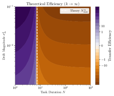
1.0.1.7 Window Algorithm as an Instance of Predictive CL
We introduce the Window algorithm as a concrete instance of our generalized CL framework: a Predictive CL algorithm that bridges both the ITL and JTL approaches through the definition of a window of tasks. At any task \(k\), the Window agent predicts the relevant future distribution with the recent \(W\) tasks and optimizes the average loss over that window, where we call \(W\) the window size. Specifically, the sampling distribution \(\mathcal{D}^k_W\) is: \[\mathcal{D}^k_W = \sum_{j = k-W+1}^k \rho_j^k \,\mathcal{P}^j \qquad \rho_j^k = \frac{|N_j|}{\sum_{i\in [k-W,k]} N_i}.\] Like the JTL agent, the Window agent’s parameters are not reset at the beginning of a new task. Clearly, as \(W\) grows, the Window agent converges to the JTL agent—which can be viewed as an infinite window agent—whereas setting \(W = 1\) recovers a variant of the ITL agent with warm starts.
1.0.1.7.1 Asymptotic Analysis in the Quadratic Loss Setting
In contrast to the JTL agent, whose stability is determined by the global growth of the task solutions relative to the origin, the Window agent’s stability depends entirely on the local variations of the environment over the horizon \(W\). To characterize this, we utilize the Mean Squared Displacement (MSD) measure.
Definition 12 (Mean Squared Displacement). Let \(m: \mathbb{N} \times \mathbb{N} \to \mathbb{R}^+\) be a function characterizing the expected squared Euclidean distance between two task solutions separated by a lag \(W\) at time \(k\): \[\mathbb{E}[\|\theta_\star^k - \theta_\star^{k-W}\|^2] \in \Theta(m(k, W)).\]
We analyze the three canonical regimes under the assumption of stationary increments. The Mean Squared Displacement scales as \(m(W) \in \Theta(1)\) for Bounded, \(\Theta(W)\) for Diffusive, and \(\Theta(W^2)\) for Linear environments.
Remark 1 (Relationship between MSD and Growth Rate). The Mean Squared Displacement is universally upper-bounded by the global growth rate: \(m(k, W) \in \mathcal{O}(\psi(k))\). This follows from the triangle inequality relative to the origin. However, for the standard regimes of interest (Diffusive and Linear), the process exhibits stationary increments. In these cases, \(m(k, W)\) depends only on the lag \(W\) and is independent of the absolute time \(k\).
1.0.1.7.2 Window Geometric Drift
The geometric drift for the Window agent is defined by the update to the sliding centroid and the shift in the stationary covariance matrix: \[\begin{align} \Delta \mu^{W,k} &= (\theta_\star^{W, k-1} - \theta_\star^{W, k}), \\ \Delta \Sigma^{W,k} &= (\Sigma_\infty^{W,k-1} - \Sigma_\infty^{W,k}). \end{align}\] Table 4 summarizes the asymptotic scaling of these drift terms. Unlike the JTL agent, where the drift is suppressed by the infinitely growing history \(k\), the Window agent’s drift is governed by the ratio of the Mean Squared Displacement to the constant window inertia \(W\).
| Mean Drift \(\mathbb{E}[\|\Delta \mu^{W,k}\|^2]\) | Covariance Drift \(\mathbb{E}[\mathrm{Tr}(\Delta \Sigma^{W,k})]\) | ||||
|---|---|---|---|---|---|
| 3-4 (l)5-6 Regime | MSD \(m(W)\) | Scaling | Vanishing? | Scaling | Vanishing? |
| Bounded | \(\Theta(1)\) | \(\mathcal{O}(W^{-2})\) | ✔ | \(\mathcal{O}(W^{-1})\) | ✔ |
| Diffusive | \(\Theta(W)\) | \(\mathcal{O}(W^{-1})\) | ✔ | \(\mathcal{O}(1)\) | \(\times\) |
| Linear | \(\Theta(W^2)\) | \(\mathcal{O}(1)\) | \(\times\) | \(\mathcal{O}(W)\) | \(\times\) |
We now present a quadratic loss analysis of the Transfer Efficiency of the Window agent compared to the ITL agent. The analysis follows the same steps as the JTL derivation, re-using several previous results.
As shown previously, the transient cost is dominated by the geometric drift of the agent’s optimum: \(\Delta \mu^{W, k} = \theta_\star^{W, k} - \theta_\star^{W, k-1}\). At step \(k\), the minimum of the Window agent objective is: \[\theta_\star^{W,k} = \left(\sum_{j=k-W}^k \rho_j^k H_j\right)^{-1} \left(\sum_{j=k-W}^k \rho_j^k H_j \theta_\star^j\right).\]
Lemma 15 (Window Geometric Drift). For a Window agent of size \(W\), the squared magnitude of the geometric mean shift scales with the growth rate of the window interval: \[\mathbb{E}[\|\Delta \mu^{W,k}\|^2] \in \Theta\left( \frac{m(k, W)}{W^2} \right).\]
Proof. Let \(\bar{H}_k = \frac{1}{W} \sum_{j \in \mathcal{W}_k} H_j\) be the average Hessian. The optimum satisfies \(\bar{H}_k \theta_\star^{W,k} = \frac{1}{W} \sum_{j \in \mathcal{W}_k} H_j \theta_\star^j\).
Comparing steps \(k\) and \(k-1\), the window \(\mathcal{W}_k\) is obtained from \(\mathcal{W}_{k-1}\) by removing task \(k-W\) and adding task \(k\). The average Hessian updates as: \[\bar{H}_k = \bar{H}_{k-1} + \frac{1}{W}(H_k - H_{k-W}).\] The weighted target vector \(v_k = \bar{H}_k \theta_\star^{W,k}\) updates as: \[v_k = v_{k-1} + \frac{1}{W}(H_k \theta_\star^k - H_{k-W} \theta_\star^{k-W}).\] Substituting \(v_{k-1} = \bar{H}_{k-1} \theta_\star^{W, k-1}\) and solving for the difference: \[\bar{H}_k \theta_\star^{W,k} = \left( \bar{H}_k - \frac{1}{W}(H_k - H_{k-W}) \right) \theta_\star^{W, k-1} + \frac{1}{W}(H_k \theta_\star^k - H_{k-W} \theta_\star^{k-W}).\] Rearranging terms to isolate the drift \(\Delta \mu^{W,k} = \theta_\star^{W,k} - \theta_\star^{W, k-1}\): \[\bar{H}_k (\theta_\star^{W,k} - \theta_\star^{W, k-1}) = \frac{1}{W} \left[ H_k (\theta_\star^k - \theta_\star^{W, k-1}) - H_{k-W} (\theta_\star^{k-W} - \theta_\star^{W, k-1}) \right].\] Multiplying by \(\bar{H}_k^{-1}\): \[\Delta \mu^{W,k} = \frac{1}{W} \bar{H}_k^{-1} \left[ H_k (\theta_\star^k - \theta_\star^{W, k-1}) + H_{k-W} (\theta_\star^{W, k-1} - \theta_\star^{k-W}) \right].\] This expression represents the pull of the new task \(k\) and the "release" of the old task \(k-W\) on the centroid. Taking the squared norm expectation and applying the bound on the condition number \(\kappa\) (3): \[\mathbb{E}[\|\Delta \mu^{W,k}\|^2] \le \frac{\kappa^2}{W^2} \mathbb{E}\left[ \left\| (\theta_\star^k - \theta_\star^{W, k-1}) + (\theta_\star^{W, k-1} - \theta_\star^{k-W}) \right\|^2 \right].\] The term inside the norm is dominated by the displacement between the incoming and outgoing tasks, \(\|\theta_\star^k - \theta_\star^{k-W}\|\). By the definition of the Mean Squared Displacement (12), the expected squared distance between two tasks separated by \(W\) steps scales as \(\Theta(m(k, W))\). Thus: \[\mathbb{E}[\|\Delta \mu^{W,k}\|^2] \in \Theta\left( \frac{m(k, W)}{W^2} \right).\] ◻
Lemma 16 (Window Covariance Drift). The geometric covariance shift for the Window agent scales asymptotically with the finite difference of the Mean Squared Displacement: \[|\mathbb{E}[\mathrm{Tr}(\Delta \Sigma^{W,k})]| \in \Theta(\Delta m(k,W)).\]
Implication: Unlike the JTL agent, the Window agent achieves a stable second moment (constant uncertainty size) because the task diversity within the active window does not grow infinitely with time \(k\).
Proof. Following the logic of 11, the stationary covariance \(\Sigma_\infty\) scales with the task diversity \(\mathcal{V}_{\text{div}}\). For the Window agent, this diversity is measured over the set \(\mathcal{W}_k\): \[\mathcal{V}_{\text{div}}^{W,k} = \frac{1}{W} \sum_{j \in \mathcal{W}_k} \|\nabla \mathcal{L}^j(\theta_\star^{W,k})\|^2 = \frac{1}{W} \sum_{j \in \mathcal{W}_k} \|\theta_\star^j - \theta_\star^{W,k}\|_{H_j^2}^2.\] This term represents the spatial variance of \(W\) consecutive tasks. The covariance shift is: \[\begin{align} \mathbb{E}[\mathrm{Tr}(\Delta \Sigma^{W,k})] &= \mathbb{E}[\mathrm{Tr}(C^{W,k-1}_\infty - C^{W,k}_\infty)]\\ &= \frac{1}{W}\left(\sum_{j \in \mathcal{W}_{k-1}} \mathbb{E}[\|\nabla \mathcal{L}^j(\theta_\star^{W,k-1})\|^2] - \sum_{j \in \mathcal{W}_k} \mathbb{E}[\|\nabla \mathcal{L}^j(\theta_\star^{W,k})\|^2]\right). \end{align}\]
Recognizing that \(\mathbb{E}[\|\nabla \mathcal{L}^j(\theta_\star^{W,k-1})\|^2] = \mathbb{E}[\|\theta_\star^j - \theta_\star^{W,k-1}\|_{H_j^2}^2]\), which is the expected norm of the average difference among the task optima in \(\mathcal{W}_{k-1}\), we know by 12 that this scales as \(\Theta(m(k-1,W))\). Similarly, \(\mathbb{E}[\|\nabla \mathcal{L}^j(\theta_\star^{W,k})\|^2] \in \Theta(m(k,W))\). Thus, asymptotically, the difference between these two scales as \(\Theta(m(k-1,W)) - \Theta(m(k,W)) =: \Delta m(k,W)\).
Overall, taking the absolute value of the trace, we have: \[|\mathbb{E}[\mathrm{Tr}(\Delta \Sigma^{W,k})]| \in \Theta(\Delta m(k,W)).\] ◻
Lemma 17 (Asymptotic Instability of the Window Agent). The expected Instability cost \(\mathcal{I}^W\) for the Window agent, which comprises the approximation bias and the stationary gradient noise, scales linearly with the Mean Squared Displacement: \[\mathbb{E}[\mathcal{I}^W] \in \Theta(m(k,W)).\]
Proof. The proof follows the same structure as 12.
The instability for the Window agent is: \[\mathcal{I}^W \approx \underbrace{\left(\mathcal{L}^k(\theta_\star^{W,k}) - \mathcal{L}^k(\theta_\star^{k})\right)}_{\text{Bias}} + \underbrace{\frac{\eta}{4B}\sum_{j=k-W}^k \rho_j^k \, \|\nabla \mathcal{L}^j(\theta_\star^{W,k})\|_{\mathcal{R}^k}^2}_{\text{Variance}}.\]
For a quadratic loss, the bias term simplifies to the weighted squared distance between the task optimum and the Window centroid: \[\mathbb{E}[\mathcal{L}^k(\theta_\star^{W,k}) - \mathcal{L}^k(\theta_\star^{k})] = \frac{1}{2} \mathbb{E}[\|\theta_\star^{W,k} - \theta_\star^k\|_{H_k}^2].\] Since \(\theta_\star^{W,k}\) is a convex combination of all tasks in the window \(k-W \dots k\), its position relative to the current task \(\theta_\star^k\) depends on the spread of the task distribution. By the definition of the Mean Squared Displacement, \(\mathbb{E}[\|\theta_\star^{W,k} - \theta_\star^k\|^2]\) scales with the maximum extent of the task boundary relative to the origin, which is \(\Theta(m(k,W))\).
The variance term reads: \[\mathbb{E}[\text{Variance}] \propto \sum_{j=k-W}^k \rho_j^k\,\, \mathbb{E}[\|H_j (\theta_\star^{W,k} - \theta_\star^j)\|_{\mathcal{R}^k}^2].\] Assuming bounded Hessians (3), this term is proportional to the variance of the task optima distribution around their mean \(\theta_\star^{W,k}\). As established in the proof of 16, this spatial variance scales exactly with the local environment growth rate \(\Theta(m(k,W))\).
Since both positive terms scale with \(\Theta(m(k,W))\), the total instability scales as \(\Theta(m(k,W))\). ◻
1.0.1.7.3 Asymptotically Optimal Window
Finally, we are ready to evaluate the asymptotic Transfer Efficiency of the Window agent and determine the optimal window choice. The following theorem mirrors the structure of 4, as the ITL baseline comparison remains exactly the same.
Lemma 18 (Asymptotic Optimality of Window Size). Let the asymptotic excess risk of the Window agent be dominated by the trade-off between task diversity and tracking lag, given by \(J(W) \asymp m(k,W) + \frac{m(k,W)}{W^2}\), where \(m(k,W)\) is the Mean Squared Displacement (MSD) of tasks within the window. The optimal window size \(W^*\) minimizing this risk depends on the environment’s non-stationarity regime:
Bounded Regime: If \(m(k,W) \in \Theta(1)\), the risk decreases monotonically with \(W\). The asymptotically optimal strategy is the JTL agent (\(W^* \to \infty\)).
Linear Drift Regime: If \(m(k,W) \in \Theta(W^2)\), the risk increases monotonically with \(W\). The asymptotically optimal strategy is the ITL agent (\(W^* = 1\)).
Diffusive Regime: If \(m(k,W) \in \Theta(W)\), the risk is strictly convex. The asymptotically optimal strategy is a Window agent with finite memory (\(1 < W^* < \infty\)).
Proof. Step 1: The Asymptotic Transfer Condition. We start from the general condition for positive transfer derived in 4. For the Window agent to outperform the Independent-Task Learning (ITL) baseline, its expected excess risk must be lower than the baseline expected risk. Let \(C^k_{\text{ITL}}\) and \(C^k_{W}\) denote the condition numbers scaling the respective bounds. The condition is: \[{\tau N \cdot \mathbb{E}[\mathcal{I}^W]} < {C^k_{\text{ITL}} \left( \mathbb{E}[\|\tilde{\mu}_0^{\text{ITL},k}\|^2] + \mathbb{E}[\text{Tr}(\tilde{\Sigma}_0^{\text{ITL},k})] \right)} - {C^k_{W} \left( \mathbb{E}[\|\tilde{\mu}_0^{W,k}\|^2] + \mathbb{E}[|\text{Tr}(\tilde{\Sigma}_0^{W,k})|] \right)}.\]
We substitute the asymptotic scaling laws derived in 17 15 16:
The expected instability \(\mathbb{E}[\mathcal{I}^W]\) scales with the local task diversity \(\Theta(m(k,W))\).
The expected centroid tracking lag \(\mathbb{E}[\|\tilde{\mu}_0^{W,k}\|^2]\) scales as \(\Theta(m(k,W)/W^2)\).
The expected covariance drift \(\mathbb{E}[|\text{Tr}(\tilde{\Sigma}_0^{W,k})|]\) scales with the change in diversity \(\Delta m(k,W) = |\Theta(m(k,W)) - \Theta(m(k-1,W))|\).
Substituting these into the inequality: \[\label{eq:full95scaling} \tau N \cdot \Theta(m(k,W)) < C^k_{\text{ITL}} \Theta(\psi(k)) - C^k_{W} \left( \Theta\left(\frac{m(k,W)}{W^2}\right) + \Theta(\Delta m(k,W)) \right).\tag{9}\]
Step 2: Optimal Window Size. To find the optimal window size \(W^*\), we isolate the terms dependent on the Window agent’s configuration. We define the asymptotic cost function \(J(W)\) as the sum of the diversity penalty (scaled by the task duration \(N\)) and the tracking lag (independent of \(N\)).
Remark on Time Dependence (\(k\)): For the canonical environments considered (Bounded, Linear Drift, Random Walk), the statistics of the task increments are stationary. Therefore, the local diversity \(m(k,W)\) within a window depends only on the window width \(W\) and not on the absolute time index \(k\). We can safely write \(m(k,W) \to m(W)\).
The cost function is defined as: \[J(W) \asymp c_1 N \cdot m(W) + c_2 \frac{m(W)}{W^2} + c_3 \Delta m(W).\] Here, \(c_1\) captures the interference cost per task, while \(c_2\) and \(c_3\) capture the mechanical lag of the tracker. We now minimize \(J(W)\) for the three canonical regimes.
1.0.1.7.3.1 Case 1: Bounded Regime.
Tasks are drawn from a fixed distribution with finite covariance: \(m(W) \sim \Theta(1)\) and \(\Delta m(W) \approx 0\). Thus, \(J(W) \sim c_1 N + \frac{c_2}{W^2}\). The term \(c_2/W^2\) is strictly decreasing while the diversity cost remains constant. Thus, \(J(W)\) is minimized as \(W \to \infty\). \[W^* = \infty \quad \text{(JTL agent is optimal)}.\]
1.0.1.7.3.2 Case 2: Linear Drift Regime.
Tasks drift with a constant velocity \(v\), i.e., \(\mathbb{E}[\|\theta_k - \theta_{k-1}\|] = v\). The variance of a line segment of length \(W\) is \(m(W) \sim \Theta(W^2)\). Because \(\frac{m(W)}{W^2} \sim \frac{W^2}{W^2} \sim \Theta(1)\), we have \(J(W) \sim c_1 N W^2 + c_2\). The diversity penalty \(N W^2\) grows quadratically, easily dominating the constant lag. The function is strictly increasing for \(W \ge 1\). \[W^* = 1 \quad \text{(ITL agent is optimal)}.\]
1.0.1.7.3.3 Case 3: Diffusive Regime.
Tasks follow a Gaussian random walk with variance \(\sigma^2\) per step. The variance grows linearly with the window size, \(m(W) \sim \Theta(W)\). The expected variance is stationary, so \(\Delta m(W) = 0\). Thus, \(J(W) \sim c_1 N W + c_2 \frac{W}{W^2} = c_1 N W + \frac{c_2}{W}\). This is a strictly convex function. We find the minimum by setting the derivative to zero: \[\frac{dJ}{dW} = c_1 N - \frac{c_2}{W^2} = 0 \implies W^2 = \frac{c_2}{c_1 N}.\] Asymptotically, the optimal window size follows the inverse square-root law: \[W^* = \sqrt{\frac{c_2}{c_1 N}} \propto \frac{1}{\sqrt{N}}.\] In this case, the optimal strategy requires a finite window. Crucially, the optimal window size shrinks as the task duration \(N\) increases. ◻
1.0.1.7.4 Window Agent for Continuously Drifting Tasks
We now explicitly instantiate this analysis for the Window agent in the continuous drift setting. Recall that the expected loss function for task \(k\) is: \[\mathcal{L}^k(\theta) = \frac{1}{2} \| \theta - \theta_\star^k \|_{\Sigma_x}^2 + \frac{1}{2}\sigma_{\xi}^2,\] where \(\|v\|_{\Sigma_x}^2 := v^\top \Sigma_x v\). The optimal parameters evolve according to a Wiener process: \[\theta_\star^k = \theta_\star^{k-1} + \Delta_k, \quad \Delta_k \sim \mathcal{N}(0, \Sigma_\Delta),\] where \(\Sigma_\Delta\) is the drift covariance matrix. At each stage \(k\), the minimizer for the Window agent is the centroid of the tasks currently inside the active window \(\mathcal{W}_k = \{k-W+1, \dots, k\}\): \[\theta_\star^{W, k} = \frac{1}{W} \sum_{j=k-W+1}^k \theta_\star^j.\]
1.0.1.7.5 Instability of the Window Agent
The instability \(\mathcal{I}^W\) measures the discrepancy between the agent’s target (the window centroid) and the true task optimum \(\theta_\star^k\), combined with the internal diversity of the window. Following the Exact Instability Decomposition (2), this splits into the centroid lag and the task scatter.
1.0.1.7.5.1 Centroid Lag.
We define the lag vector \(v_W := \theta_\star^{W, k} - \theta_\star^k\). Using the backward recursion \(\theta_\star^j = \theta_\star^k - \sum_{m=j+1}^k \Delta_m\), we substitute this into the centroid definition: \[v_W = \frac{1}{W} \sum_{j=k-W+1}^k \left( \theta_\star^k - \sum_{m=j+1}^k \Delta_m \right) - \theta_\star^k = - \frac{1}{W} \sum_{j=k-W+1}^k \sum_{m=j+1}^k \Delta_m.\] Rearranging the double sum to group by the individual increment \(\Delta_p\) (where each \(\Delta_p\) appears for all tasks \(j < p\)): \[v_W = - \frac{1}{W} \sum_{p=1}^{W-1} p \Delta_{k-p+1}.\] The expected energy of the lag is the weighted sum of the increment covariances. Using the approximation \(\sum_{p=1}^{W-1} p^2 \approx W^3/3\) for large \(W\): \[\mathbb{E}[\| v_W \|_{\Sigma_x}^2] = \text{Tr}\left( \Sigma_x \frac{1}{W^2} \sum_{p=1}^{W-1} p^2 \Sigma_\Delta \right) \approx \frac{W}{3}\text{Tr}(\Sigma_x \Sigma_\Delta).\] This term represents the irreducible tracking error; the centroid inherently lags behind the random walk by a distance proportional to the window size.
1.0.1.7.5.2 Diversity Noise.
The second component of instability is the scatter of task optima within the window. Using the identity \(\sum (x_i - \bar{x})^2 = \frac{1}{2W}\sum_{i,j}(x_i - x_j)^2\), we write the sum of squared errors as: \[\sum_{j \in \mathcal{W}_k} \|\theta_\star^{W,k} - \theta_\star^j\|_{\Sigma_x^2}^2 = \frac{1}{2W} \sum_{i,j \in \mathcal{W}_k} \|\theta_\star^i - \theta_\star^j\|_{\Sigma_x^2}^2.\] For a random walk, the expected squared distance scales with the time lag \(|i-j|\): \[\mathbb{E}[\|\theta_\star^i - \theta_\star^j\|_{\Sigma_x^2}^2] = |i-j|\text{Tr}(\Sigma_x^2 \Sigma_\Delta).\] Summing this over the window indices (using \(\sum_{i,j=1}^W |i-j| \approx W^3/3\)): \[\mathbb{E}\left[ \sum_{j \in \mathcal{W}_k} \|\theta_\star^{W,k} - \theta_\star^j\|_{\Sigma_x^2}^2 \right] \approx \frac{1}{2W} \left( \frac{W^3}{3} \right) \text{Tr}(\Sigma_x^2 \Sigma_\Delta) = \frac{W^2}{6} \text{Tr}(\Sigma_x^2 \Sigma_\Delta).\] Finally, we substitute this into the instability decomposition. Note that the instability term averages this sum over the \(W\) tasks (introducing a \(1/W\) coefficient): \[\begin{align} \mathbb{E}[\mathcal{I}^W] &\approx \frac{1}{2}\mathbb{E}[\| v_W \|_{\Sigma_x}^2] + \frac{\eta}{4 B W} \mathbb{E}\left[ \sum_{j \in \mathcal{W}_k} \|\theta_\star^{W,k} - \theta_\star^j\|_{\Sigma_x^2}^2 \right] \\ &= \frac{1}{2}\left(\frac{W}{3}\text{Tr}(\Sigma_x \Sigma_\Delta)\right) + \frac{\eta}{4 B W} \left(\frac{W^2}{6} \text{Tr}(\Sigma_x^2 \Sigma_\Delta)\right) \\ &= \frac{W}{6} \text{Tr}(\Sigma_x \Sigma_\Delta) + \frac{\eta W}{24B} \text{Tr}(\Sigma_x^2 \Sigma_\Delta). \label{eq:window95instability} \end{align}\tag{10}\]
1.0.1.7.6 Transient Error of the Window Agent
The Transient Error \(\delta^W\) arises from the initialization error at the start of each task. The Window agent initializes at the previous centroid \(\theta_\star^{W, k-1}\). The expected error vector \(\tilde{\mu}_0^{W,k}\) is driven entirely by the geometric shift in the centroid itself: \[\Delta \mu_W = \theta_\star^{W, k} - \theta_\star^{W, k-1} = \frac{1}{W} \left( \sum_{j=k-W+1}^k \theta_\star^j - \sum_{j=k-W}^{k-1} \theta_\star^j \right) = \frac{1}{W} (\theta_\star^k - \theta_\star^{k-W}).\] This shift collapses to the average of the \(W\) increments that separate the new incoming task from the one exiting the window: \[\Delta \mu_W = \frac{1}{W} \sum_{m=k-W+1}^k \Delta_m.\] The expected squared norm of this drift is: \[\mathbb{E}[\|\Delta \mu_W\|^2] = \frac{1}{W^2} \sum_{m=1}^W \text{Tr}(\Sigma_\Delta) = \frac{1}{W} \text{Tr}(\Sigma_\Delta).\] Following the exact same logic as in 1.0.1.6.3, the expected initialization error \(\tilde{\mu}_0\) tracks this input drift with an amplification factor \(c_\mu = \frac{1}{1-\rho_\mu}\). Unlike the JTL agent, the Window agent’s target covariance is stationary in expectation (i.e., zero expected covariance drift), meaning the Transient Error is dominated purely by the centroid shift. Using the bound form derived in 4: \[\mathbb{E}[\delta^W] \approx \frac{\gamma_{\max}}{\tau N} c_\mu^2 \mathbb{E}[\|\Delta \mu_W\|^2] = \frac{\gamma_{\max}}{\tau N} \frac{c_\mu^2}{W} \text{Tr}(\Sigma_\Delta).\]
1.0.1.7.7 The Optimal Window \(W^\star\)
To determine the optimal window size, we minimize the total asymptotic risk contributed by the Window agent. This risk is composed of the diversity cost (the Instability), which grows with \(W\), and the Transient Error cost, which shrinks with \(W\): \[W^\star = \arg \min_W \left[ \underbrace{ \mathbb{E}[\mathcal{I}^W]}_{\text{Instability Cost}} + \underbrace{\mathbb{E}[\delta^W]}_{\text{Transient Cost}} \right].\] Substituting the derived expressions and extracting the explicit dependence on \(W\): \[W^\star = \arg \min_W \left[ W \cdot \underbrace{ \left( \frac{\text{Tr}(\Sigma_x \Sigma_\Delta)}{6} + \frac{\eta \text{Tr}(\Sigma_x^2 \Sigma_\Delta)}{24B} \right)}_{\mathcal{R_B}} + \frac{1}{W} \cdot \underbrace{\frac{\gamma_{\max} c_\mu^2 \sigma^2_\Delta}{\tau N}}_{\mathcal{R_T}} \right].\] The objective function is of the form: \[f(W) = \mathcal{R_B} W + \mathcal{R_T} W^{-1},\] which is strictly convex. The minimum is achieved at the square-root balance: \[W^\star = \sqrt{\mathcal{R_T} / \mathcal{R_B}}.\]
Written explicitly, the optimal window length is: \[\begin{align} \label{eq:optimal-window} W^\star &= \sqrt{\frac{\gamma_{\max} c_\mu^2 \sigma^2_\Delta / (\tau N)}{\frac{\text{Tr}(\Sigma_x \Sigma_\Delta)}{6} + \frac{\eta \text{Tr}(\Sigma_x^2 \Sigma_\Delta)}{24B} }} \\ &= \frac{c_\mu \,\sqrt{{\gamma_{\max}}}}{\sqrt{\tau N}} \left(\frac{\text{Tr}(\Sigma_x \Sigma_\Delta)}{6\,\sigma^2_\Delta} + \frac{\eta \text{Tr}(\Sigma_x^2 \Sigma_\Delta)}{24B\,\sigma^2_\Delta}\right)^{-1/2}. \end{align}\tag{11}\] This exact, non-asymptotic result perfectly aligns with the asymptotic scaling derived in 17, confirming that \(W^\star \propto N^{-1/2}\).
1.0.2 Empirical Setup↩︎
1.0.2.1 Simulations
All simulations are implemented in JAX to heavily vectorize training over multiple random seeds and hyperparameter grids, ensuring statistically robust results.
1.0.2.1.1 Shallow Linear Experiments
To validate our exact analytical derivations for the continuous drift setting, we simulate a sequence of linear tasks tracking a random walk. The input dimension is \(d=10\). Data inputs are sampled as \(x \sim \mathcal{N}(0, I)\), and task labels are generated by a teacher \(\theta_\star^k\) as \(y = x^\top \theta_\star^k + \xi\), where \(\xi \sim \mathcal{N}(0, \sigma_\xi^2)\). The teacher undergoes a random walk such that \(\theta_\star^k = \theta_\star^{k-1} + \Delta_k\), with \(\Delta_k \sim \mathcal{N}(0, \frac{\sigma_\Delta^2}{d} I)\).
We sweep over the two main axes of our phase diagram:
Task Duration (\(N\)): Swept geometrically.
Drift Magnitude (\(\sigma_\Delta^2\)): Swept logarithmically.
The models are trained using stochastic gradient descent (SGD) with a constant learning rate (e.g., \(\eta=0.1\)). We compute the exact Transfer Efficiency between the Independent-Task Learning (ITL) and Joint-Task Learning (JTL) agents averaged over \(K\) tasks and \(40\) random seeds, and overlay the theoretical breakeven boundary directly onto the empirical phase transitions to verify our non-asymptotic bounds.
1.0.2.1.2 Deep Linear Experiments
To analyze the scaling dynamics and the impact of the loss landscape, we extend the experiments to deep linear networks. We use a teacher-student setup with a depth-3 linear network, an input dimension of \(d=10\), and an output dimension of \(1\). The hidden width is swept across \(m \in \{32, 64, 128, 256, 512, 1024\}\).
The teacher network’s weights are initialized randomly and undergo a continuous random walk to induce task drift. We fix the total drift magnitude to \(\sigma_\Delta^2 = 0.05\). Only three tasks are trained to isolate the initial transient and instability dynamics, with each task lasting for exactly \(N=500\) steps. We use a batch size of \(B=32\) and a label noise standard deviation of \(\sigma_\xi=0.01\).
The Independent-Task Learning (ITL) agent simply continues training on the incoming data stream, while the Joint-Task Learning (JTL) agent utilizes exact experience replay, uniformly sampling its batches from the current and all previously seen tasks.
We evaluate two different initialization and scaling regimes. Let the hidden width be denoted by \(m\), and let the three trainable matrices be \(U \in \mathbb{R}^{d \times m}\), \(V \in \mathbb{R}^{m \times m}\), and \(a \in \mathbb{R}^{m \times 1}\), with all entries initialized i.i.d. as \(\mathcal{N}(0,1)\). For an input \(x \in \mathbb{R}^d\), the depth-3 linear network is implemented as \[h_1(x) = \frac{xU}{\sqrt{d}}, \qquad h_2(x) = \frac{h_1(x)V}{\sqrt{m}}, \qquad f_\Theta(x) = \frac{h_2(x)a}{\sqrt{m}\,\gamma_m}.\] Thus the input and hidden matrix multiplications use fan-in normalization, while the scalar factor \(\gamma_m\) controls the output scale of the parametrization. The same parametrization is used for the teacher and the student networks.
The two regimes differ only in the output multiplier \(\gamma_m\) and the learning-rate multiplier \(s_\eta(m)\) applied to the base learning rate:
NTK parametrization (NTP). We set \(\gamma_m = 1\) and \(s_\eta(m)=1\), so the effective SGD learning rate is independent of width. This is the neural-tangent scaling used to approach lazy kernel dynamics in the wide-network limit: as \(m\) grows, the network function changes mainly through the linearization around initialization, and the hidden representation moves by a vanishing amount [23], [57].
Maximal Update parametrization (\(\mu\)P). We set \(\gamma_m=\sqrt{m}\) and multiply the base learning rate by \(s_\eta(m)=m/m_0\), where the base width is \(m_0=32\). Equivalently, compared with the NTK/NTP run, the output is scaled down by an additional factor \(\sqrt{m}\) while the optimizer step size is scaled up linearly with width. This is the maximal-update parametrization: under width scaling, hidden-layer updates remain large enough to produce feature learning, and learning-rate choices transfer more stably across widths [57], [58].
We sweep the base learning rate logarithmically from \(10^{-3}\) to \(10^1\) across \(15\) values. We observe hyperparameter transfer in \(\mu\)P as expected, meaning the optimal learning rate remains stable across widths, whereas it shifts significantly in NTP. To ensure a fair comparison, the learning rate for the ITL agent is chosen based on the first task’s performance, while the learning rate for the JTL agent is chosen based on the last task’s performance (lowest loss). All grid points are averaged over \(5\) random seeds.
The loss curves with the best selected learning rate are depicted in the figures below.
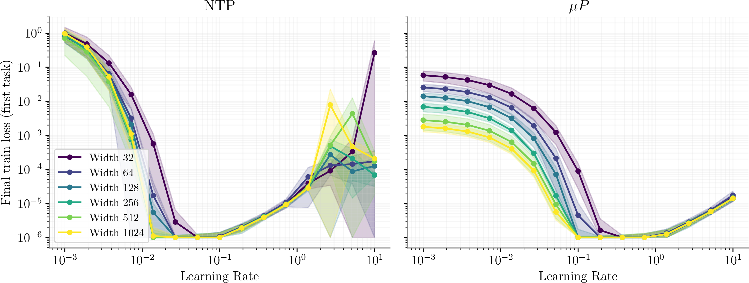
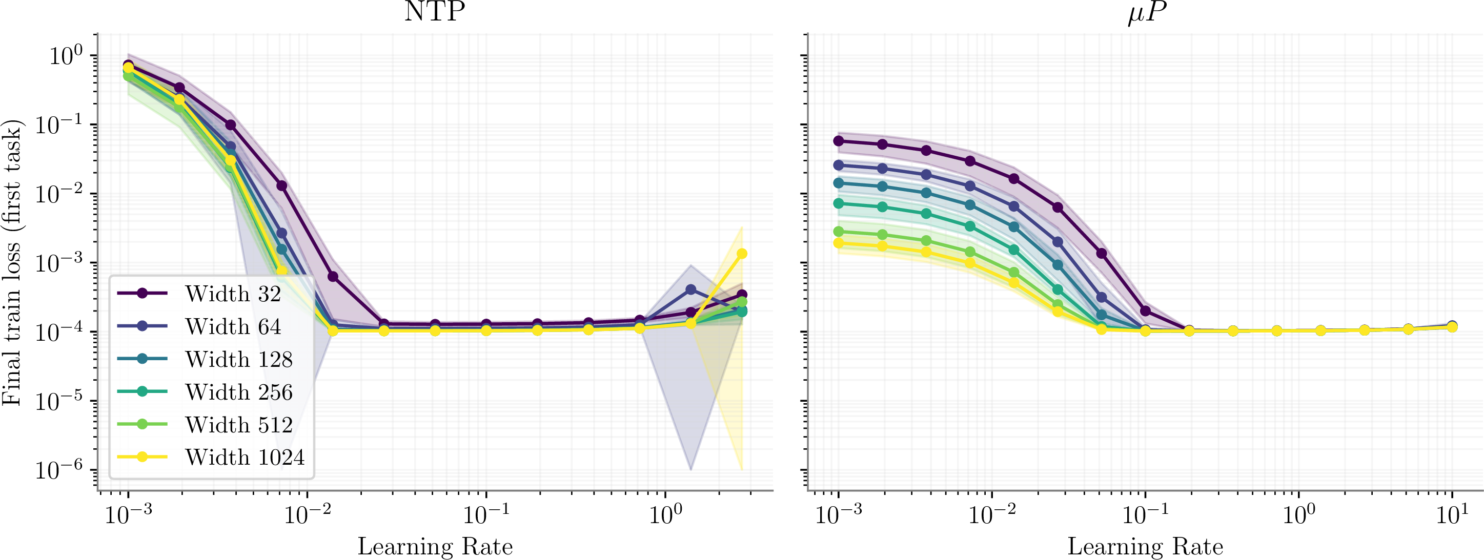
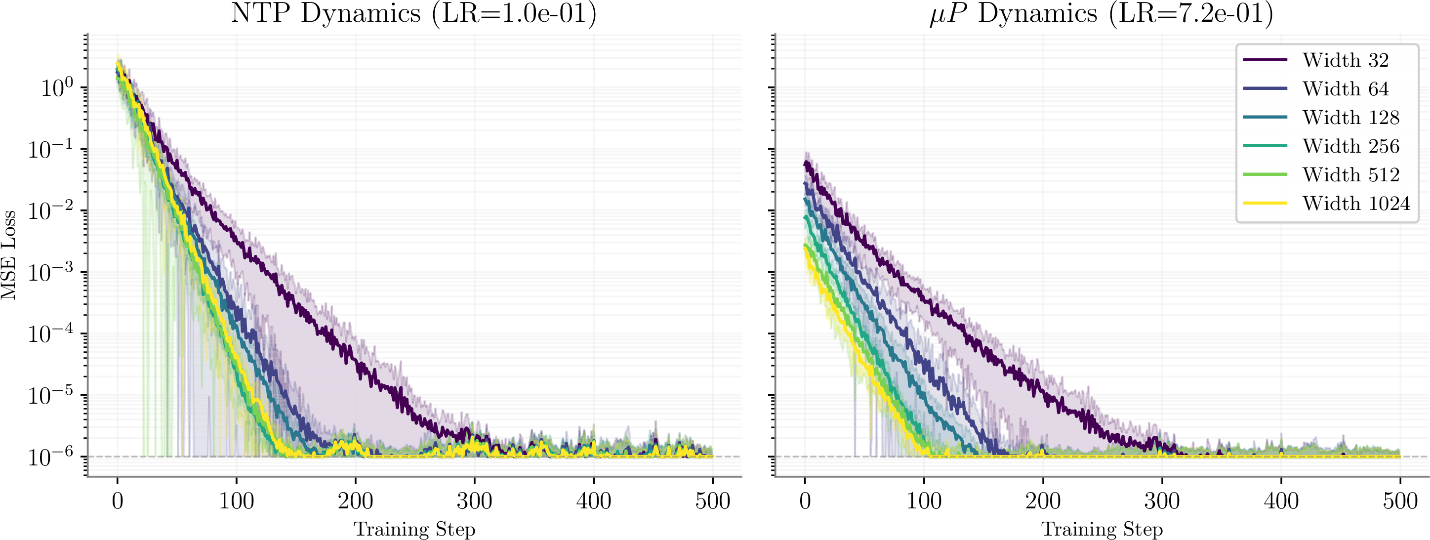
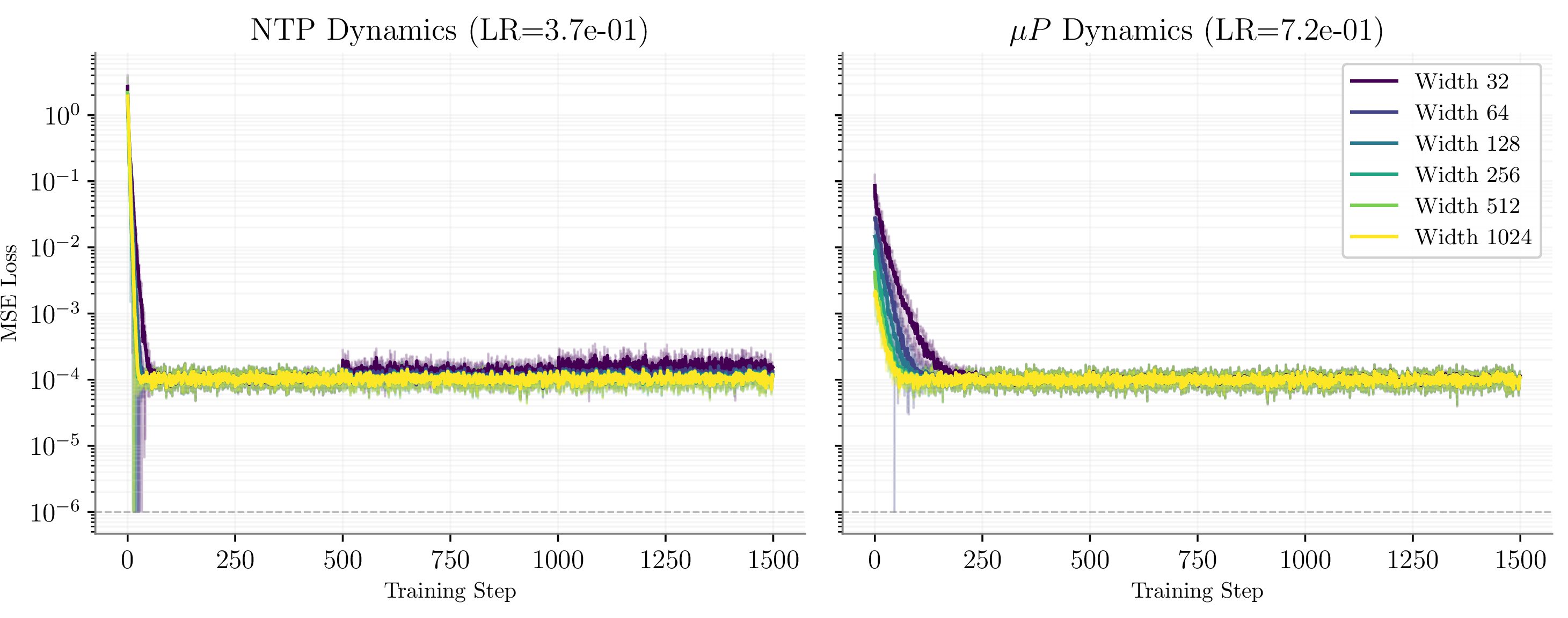
1.0.2.1.3 Window Predictive CL Algorithm Experiments
To empirically validate our non-asymptotic derivations for the Window Predictive CL algorithm (1.0.1.7), we implement the Window agent in the shallow linear continuous drift environment. The Window agent optimizes a uniformly weighted mixture of the past \(W\) tasks, \(\mathcal{D}^k_W = \frac{1}{W} \sum_{j = k-W+1}^k \mathcal{P}^j\).
Our experiments for the Window agent are divided into two primary evaluations:
1.0.2.1.3.1 Real-Time Trajectory Evaluation with \(W^\star\):
First, we test the predictive power of our theoretical optimal window formula (11 ). For a given task duration \(N\), we compute the theoretical optimum \(W^\star\) using the environment and optimizer parameters (e.g., drift magnitude \(\sigma_\Delta^2\), learning rate \(\eta\), batch size \(B\), and input covariance \(\Sigma_x\)). We then simulate the full training trajectory of the Independent-Task Learning (ITL) agent, the Joint-Task Learning (JTL) agent, and the Window agent explicitly parameterized with \(W = W^\star\). We average the test loss over multiple seeds and smooth the curves by averaging over the task duration \(N\) to clearly visualize the transient and stationary phases of adaptation.
1.0.2.1.3.2 Transfer Efficiency Landscapes:
Second, we rigorously map the space of positive transfer to show how the environment’s non-stationarity limits the optimal memory horizon. We fix the task duration to distinct scales (e.g., \(N \in \{100, 500, 1000\}\)) and perform a 2D grid search over:
Window Size (\(W\)): Swept across a discrete range of integer values.
Drift Magnitude (\(\sigma_\Delta^2\)): Swept logarithmically.
For every point in this grid, we compute the exact Average Task Error (\(\mathrm{ALE}^k\)) over a long sequence of tasks (e.g., \(K=100\)) to bypass initial task transient effects. We then calculate the Transfer Efficiency (TE) relative to the ITL baseline. This generates the 2D heatmaps (shown in 15), which empirically verify our claims that (1) the area of positive transfer shrinks as task duration and drift increase, and (2) overly large window sizes introduce detrimental bias in highly non-stationary regimes, pulling the optimal \(W\) toward \(1\).
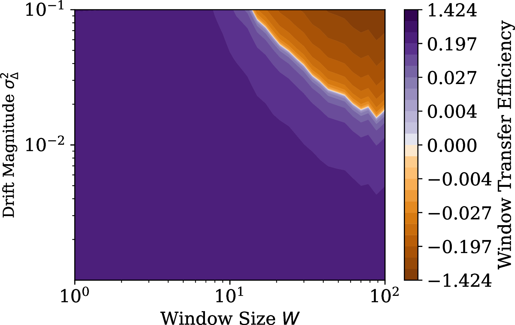
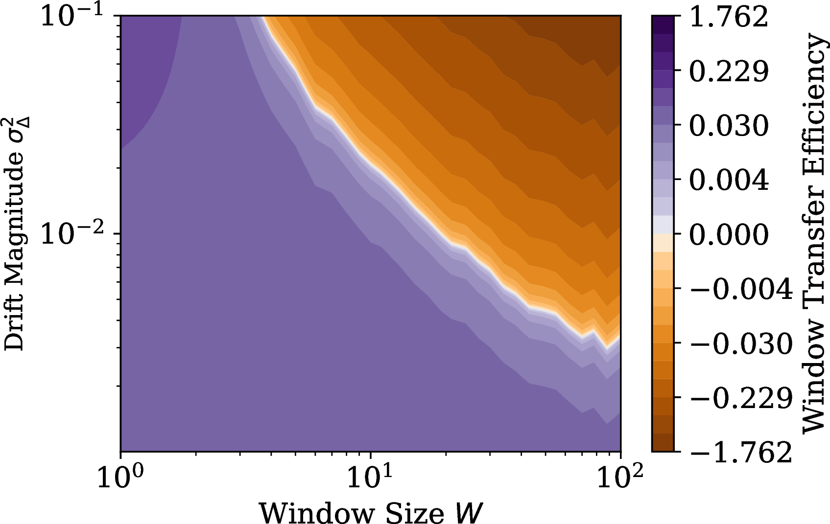
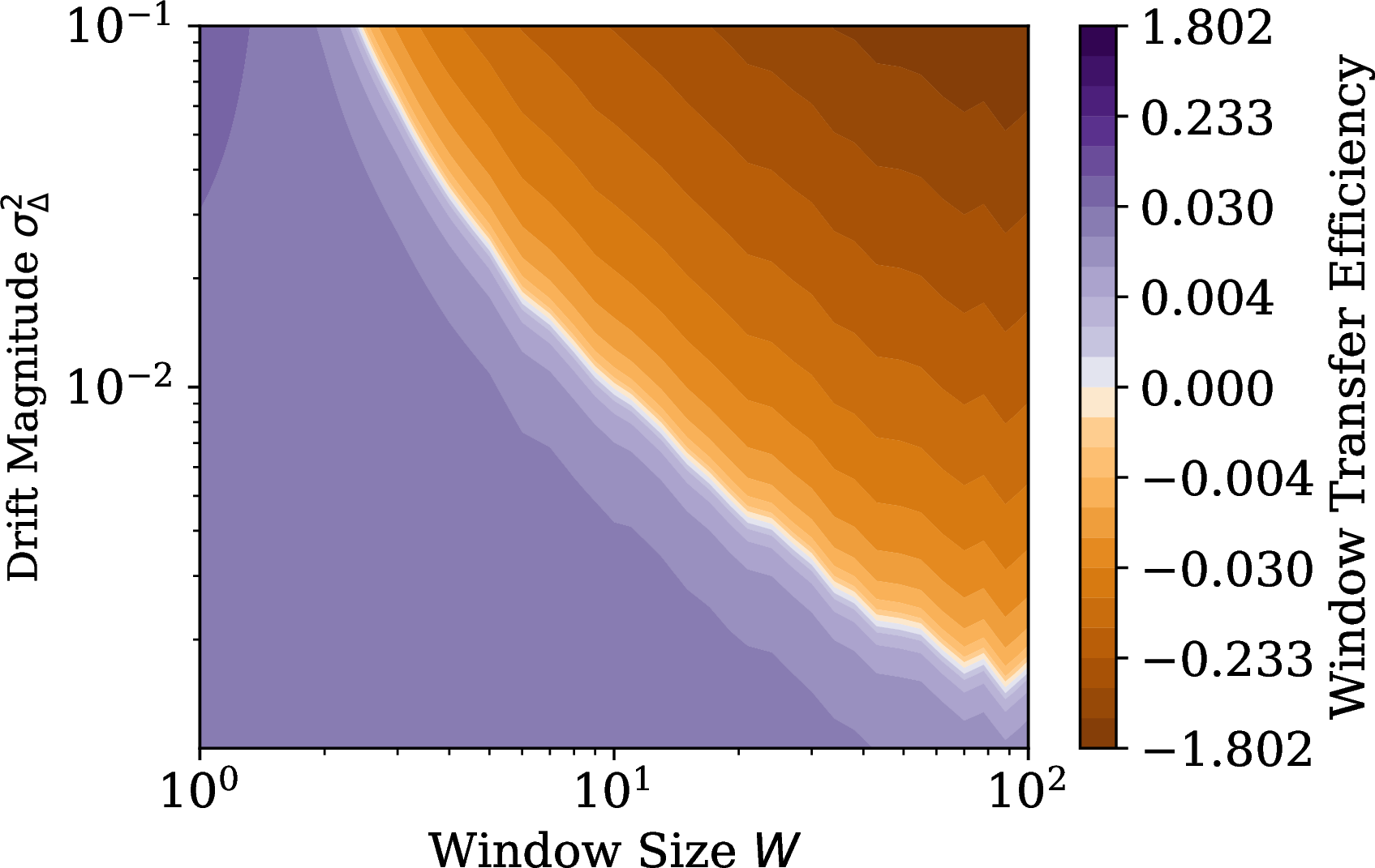
Figure 15: Transfer Efficiency Landscape for the Window Agent. The grids display the Transfer Efficiency of the Window agent as a function of Window Size \(W\) (x-axis) and Drift Magnitude \(\sigma_\Delta^2\) (y-axis). From left to right, the task duration increases (\(N = 100, 500, 1000\)). The area of positive transfer (white to orange) shrinks significantly as both task duration and drift magnitude increase. This visually confirms the theoretical analysis: overly large window sizes introduce a detrimental bias in highly non-stationary or long-duration environments, pulling the optimal \(W^\star\) toward \(1\)..
1.0.2.2 Real-World Benchmarks
| Benchmark | Tasks (\(K\)) | Input Size | Classes | Samples per Task (\(N_k\)) |
|---|---|---|---|---|
| CLEAR | 10 | 224\(\times\)224 | 100 | \(\approx 109\)K |
| MD5 | 5 | 224\(\times\)224 | 30 | \(\in[1480, 27750]\) |
| P/S CIFAR10 | 10 | 32\(\times\)32 | 10 | \(10\)K |
| Dataset | Original Classes | Total Samples |
|---|---|---|
| StanfordCars | 196 | 1523 |
| FGVCAircraft | 100 | 2467 |
| DTD | 47 | 1480 |
| Food101 | 101 | 27750 |
| OxfordPet | 37 | 3680 |
1.0.2.2.1 CLEAR
The CLEAR dataset [20] is a collection of images spanning the years 2004–2014, designed to evaluate models under natural temporal distribution shifts. We utilize the 100-class variant and split the collection into \(K=10\) distinct tasks, one for each year. The tasks are organized in their natural temporal ordering. All input images are resized to 224\(\times\)224 pixels and normalized by subtracting the ImageNet mean \(\mu = [0.485, 0.456, 0.406]\) and dividing by the standard deviation \(\sigma = [0.229, 0.224, 0.225]\).

1.0.2.2.2 MULTIDATASET (MD5)
The MULTIDATASET benchmark consists of a sequence of \(K=5\) distinct open-source classification datasets with no semantic overlap. Specifically, the tasks consist of classifying automobile models [59], aircraft models [60], textures [61], dishes [62], and pets [63]. Each dataset originally features a different number of classes, samples, and input resolutions (detailed in 6).
To prevent the introduction of architectural biases or capacity imbalances, we standardize all tasks to have exactly 30 classes. Furthermore, we enforce identical batch sizes and total update steps across tasks, regardless of the original dataset’s size. All input images are resized to 224\(\times\)224 pixels and normalized using the standard ImageNet statistics (\(\mu = [0.485, 0.456, 0.406]\), \(\sigma = [0.229, 0.224, 0.225]\)). During training, the data is augmented with random crops, random horizontal flips, and random rotations of up to 15 degrees.
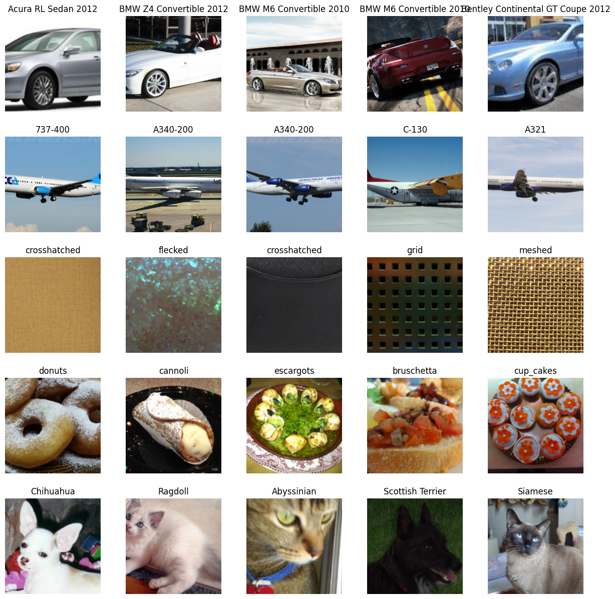
1.0.2.2.3 Meta-World
Meta-World [21] is a suite of simulated robotic manipulation tasks built on the MuJoCo physics engine. Our experiments use the MT10
benchmark, a fixed collection of \(10\) distinct manipulation tasks (reach, push, pick-place, door-open, drawer-open, drawer-close, button-press-topdown,
peg-insert-side, window-open, window-close) on the shared Sawyer robot. We use the v3 environment versions provided by the official Meta-World release. Unlike the meta-learning split (ML10), MT10 is designed for
multi-task and continual evaluation on a common task set, with no held-out tasks.
At each step, the environment yields a \(39\)-dimensional observation vector that includes the robot’s joint positions, the gripper state, and the spatial coordinates of relevant objects, with the goal position
zero-masked. For the JTL agent, this observation is concatenated with a \(10\)-dimensional one-hot task identifier, yielding a \(49\)-dimensional input. The agent emits a \(4\)-dimensional continuous action (end-effector delta plus gripper command), with components squashed to \([-1, 1]\) via a \(\tanh\). Each episode lasts at most
\(500\) time steps and yields a binary success flag in addition to the shaped reward.
1.0.2.3 Synthetic Benchmarks
1.0.2.3.1 Permuted CIFAR-10
Permuted CIFAR-10 is a benchmark constructed from the standard CIFAR-10 dataset [64] by applying fixed random spatial permutations to the images. We utilize two different permutation severities in our experiments, defined by the spatial dimensions of the perturbed area: 16\(\times\)16 and 32\(\times\)32. These denote the side length of the square patch of pixels—centered in the image—that undergoes the random permutation (see 18 (a) and 18). We refer to these respective benchmarks as ‘PC-16’ and ‘PC-32’. All input images are normalized by subtracting the mean \(\mu = [0.507, 0.486, 0.441]\) and dividing by \(\sigma = [0.267, 0.256, 0.276]\).
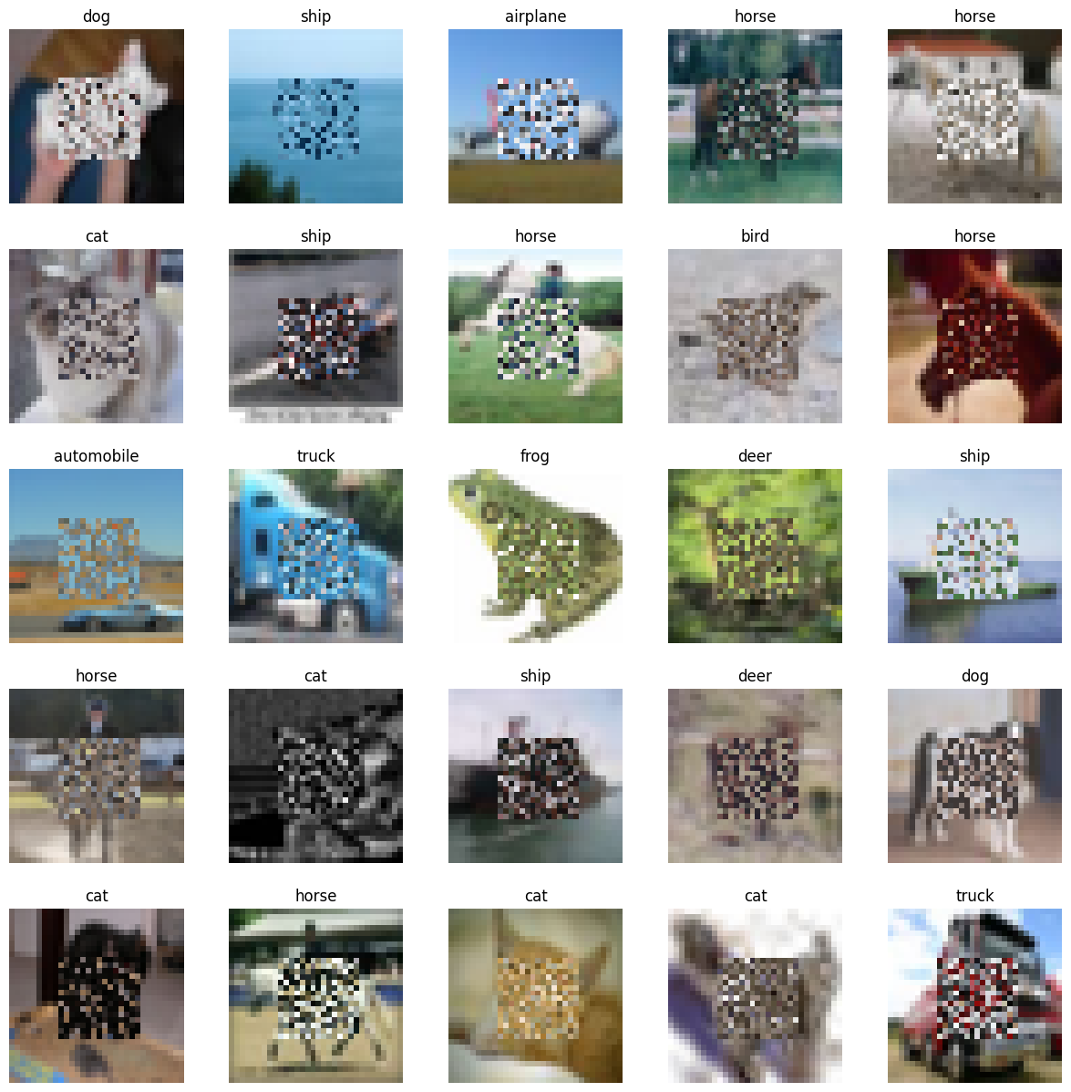

Figure 18: Samples from a Permuted CIFAR-10 task with a 32\(\times\)32 permutation box.. a — Samples from a Permuted CIFAR-10 task with a 16\(\times\)16 permutation box.
1.0.2.3.2 Shuffled CIFAR-10
Shuffled CIFAR-10 is an alternative benchmark built from the CIFAR-10 dataset [64], which isolates the effect of concept drift by applying targeted label resampling to a set of samples fixed at the beginning of training. We sweep the proportion of shuffled labels across three severities: 10%, 30%, and 50%. To guarantee that this injected label noise is strictly adversarial, we prevent the true label from being drawn during the reshuffling process. We refer to these benchmarks as ‘SC-10’, ‘SC-30’, and ‘SC-50’. Input images are normalized using the same statistics as Permuted CIFAR-10. Crucially, because the labels are irreversibly corrupted in the training set, we evaluate the resulting generalization penalty on the uncorrupted test set.
1.0.2.4 Training Procedures & Networks
1.0.2.4.0.1 Supervised Learning
All supervised learning agents consist of a deep neural network backbone, an optimizer, and a learning rate scheduler. Across all supervised experiments, the core architecture is a ResNet-18 (RN18). The output dimension of the final linear classification head is set to the total number of classes in the respective benchmark (100 for CLEAR, 30 for MD5, and 10 for Permuted/Shuffled CIFAR-10), and this head is shared across all tasks. Both the Independent-Task Learning (ITL) and Joint-Task Learning (JTL) agents are trained for an identical number of gradient steps \(h\) per task. General optimization configurations are detailed in 7, with explicitly tuned hyperparameters listed in 8.
ITL Agent. Given a sequence of \(K\) tasks, the ITL agent is trained to minimize the cross-entropy loss exclusively on the training data of the current active task. To establish a strict ITL baseline and prevent any forward transfer, both the network weights and the optimizer state of the ITL agent are completely re-initialized to their random starting priors at the beginning of every task.
JTL Agent. The JTL agent minimizes the expected loss over the union of all currently and previously observed tasks. In practice, this is implemented using an exact experience replay buffer: at each gradient step, the optimizer processes a concatenated batch comprising data from the current task stream alongside data uniformly sampled from the buffer of previous tasks. Unlike the ITL agent, the JTL agent’s network parameters and optimizer state are preserved across task boundaries.
1.0.2.4.0.2 Reinforcement Learning
In our reinforcement learning experiments, we compare ITL and JTL agents using Soft Actor-Critic (SAC) [65] on the MT10 subset of the Meta-World benchmark [21], with automatic entropy temperature tuning [66]. SAC is the standard off-policy continuous-control algorithm used in the multi-task Meta-World literature [21], and its use of a single replay buffer makes the ITL and JTL agents differ only in (i) what data populates the buffer and (ii) whether the policy is conditioned on a task identifier; the underlying optimizer, network architecture, and per-epoch compute budget are otherwise identical.
Architecture (shared). For both agents, the actor and the twin critics are MLPs with two hidden layers of \(400\) units and ReLU activations. The actor outputs the mean and (clipped) log-standard-deviation of a diagonal Gaussian, squashed by \(\tanh\); the critics output a scalar \(Q\)-value. The log-std is clipped to \([-20, 2]\).
ITL Agent. For each task in MT10 we train a separate SAC agent from a random initialization, with its own replay buffer and its own learned entropy temperature \(\alpha\). The agent observes only the 39-dimensional Meta-World state of its task; no task identifier is appended. Each ITL run lasts \(500\) epochs; per epoch we collect \(40\) rollouts of length \(500\) (\(2 \times 10^{4}\) environment steps) into the buffer and then perform \(500\) SAC gradient updates with mini-batch size \(500\).
JTL Agent. We train a single SAC agent across all MT10 tasks under a curriculum: at epoch \(e\) the active set is the first \(1 + \lfloor e / N \rfloor\) tasks in a fixed ordering, with task duration \(N = 500\) epochs. The actor and critics are conditioned on a \(10\)-dimensional one-hot task identifier concatenated to the observation. A single replay buffer of capacity \(10^{6}\) is shared across all tasks and is never reset; whenever a new task becomes active we re-initialize the Adam states of the actor and critic optimizers (the entropy temperature is kept) so that the optimizer can adapt to the new objective. Per epoch we collect \(200\) rollouts of length \(500\) (\(10^{5}\) environment steps) by uniformly cycling over the currently active environments, then perform \(500\) SAC gradient updates with mini-batch size \(500\) sampled uniformly from the shared buffer. Evaluation each epoch is performed on the current task.
Task ordering. For the curriculum experiments shown in the main paper we use the easy_to_hard ordering, obtained by sorting MT10 tasks in decreasing order of the final single-task success rate of the ITL SAC agents under the same
configuration. The resulting sequence is drawer-close, window-close, button-press-topdown, drawer-open, reach, window-open, door-open, push,
peg-insert-side, pick-place. Each configuration (ITL and JTL) is replicated over \(10\) seeds; per-task figures aggregate seeds for which the entire \(500\)-epoch
stage is logged, with a minimum of \(7\) seeds per relative epoch.
1.0.2.4.1 Hyperparameters
1.0.2.4.1.1 Supervised Learning
The key hyperparameters—learning rate and weight decay—are carefully tuned separately for each combination of agent and benchmark using a grid search. To ensure a fair comparison, the optimizer and scheduler dynamics are fixed across most supervised learning experiments. We employ Stochastic Gradient Descent (SGD) paired with a task-wise Cosine Annealing scheduler. Specifically, the learning rate is smoothly annealed toward zero over the course of each task’s duration (\(h\) steps) and undergoes a hard reset to its maximum initial value at the beginning of the next task, providing the necessary plasticity to rapidly minimize the changing objective.
| Hyperparameter | Value |
|---|---|
| Optimizer | SGD |
| Momentum | 0.9 |
| Scheduler | Cosine Annealing (Task-wise) |
| Stream Batch Size | 256 |
| Dataset | Agent | Network | LR | Weight Decay | |
|---|---|---|---|---|---|
| CLEAR | ITL | RN18 | 0.100 | \(3 \times 10^{-4}\) | |
| CLEAR | JTL | RN18 | 0.100 | \(1 \times 10^{-4}\) | |
| PC-16 | ITL | RN18 | 0.055 | \(8 \times 10^{-4}\) | |
| PC-16 | JTL | RN18 | 0.075 | \(7 \times 10^{-4}\) | |
| PC-32 | ITL | RN18 | 0.060 | \(1 \times 10^{-3}\) | |
| PC-32 | JTL | RN18 | 0.074 | \(1 \times 10^{-3}\) | |
| MD5 | ITL | RN18 | 0.089 | \(9 \times 10^{-4}\) | |
| MD5 | JTL | RN18 | 0.080 | \(6 \times 10^{-4}\) |
1.0.2.4.1.2 Reinforcement Learning
For a fair comparison, ITL and JTL share the same SAC core hyperparameters (network width, learning rates, \(\gamma\), \(\tau\), entropy auto-tuning, mini-batch size, and the number of SAC gradient updates per epoch). The two agents differ only along axes that are intrinsic to the ITL/JTL distinction: (i) the size of the rollout collected per epoch (\(2 \times 10^{4}\) environment steps for ITL on its single active task vs.\(10^{5}\) for JTL split uniformly over the currently active tasks), (ii) the presence of a one-hot task conditioning for JTL, (iii) replay buffer scope (per-task vs.shared across the curriculum), and (iv) optimizer state at task boundaries (full re-initialization at every task for ITL vs.Adam-state reset of actor/critic only when a new task becomes active for JTL). All optimization is performed with Adam. Here compute-matched refers to the gradient-update budget—the number of SAC updates (\(500\)) and the mini-batch size (\(500\)) per epoch are identical for the two agents—rather than the environment-step count, which differs by construction (\(2\times10^{4}\) steps per epoch for ITL on its single task vs.\(10^{5}\) for JTL split over the active tasks); if anything, JTL is given more environment data per epoch, yet still underperforms.
We follow the MT-SAC configuration of [21] for the shared core, with the ITL-side cycle/rollout schedule taken from the single-task SAC appendix of the same work. The resulting hyperparameters are reported in 9; per-task and per-curriculum runtime budgets follow directly from the rollout schedule and the number of gradient updates.
| Parameter | ITL | JTL |
|---|---|---|
| Shared SAC core (identical for ITL and JTL) | ||
| Optimizer | Adam | |
| Hidden layers (actor / critic) | \(2 \times 400\) | |
| Activation | ReLU | |
| Actor / critic / \(\alpha\) learning rate | \(3 \times 10^{-4}\) | |
| Discount \(\gamma\) | \(0.99\) | |
| Target smoothing \(\tau\) | \(5 \times 10^{-3}\) | |
| Entropy temperature \(\alpha\) | auto-tuned | |
| \(\log \sigma\) clip | \([-20,\;2]\) | |
| SAC mini-batch size | \(500\) ([tbl:tab:results-wild]); \(5000\) (ablation) | |
| Gradient updates per epoch | \(500\) | |
| Epochs per task (\(N\)) | \(500\) | |
| ITL / JTL-specific | ||
| Task conditioning | none | one-hot, \(\mathbb{R}^{10}\) |
| Episodes per epoch (length \(500\)) | \(40\) | \(200\) |
| Env.steps per epoch | \(2 \times 10^{4}\) | \(10^{5}\) |
| Replay buffer | per task | shared, capacity \(10^{6}\) |
| Min.buffer size before updates | \(1{,}500\) | \(1{,}500\) |
| Buffer reset at task switch | yes | no |
| Optimizer reset | full reset every task | Adam state of actor/critic re-init (\(\alpha\) kept) |
| Curriculum / ordering | N/A | easy_to_hard |
| Eval target each epoch | current task | current task |
| Number of seeds | \(10\) | \(10\) |
Effect of the SAC mini-batch size on ITL agents. We fix the SAC mini-batch size to \(500\) for both ITL and JTL so that the two agents share an identical per-update compute budget (9). Since the quadratic analysis predicts that the optimization-induced (Variance) penalty scales as \(1/B\) in the batch size \(B\) (0.0.4), it is natural to ask whether the absolute performance of the agents, and hence the task-difficulty ordering that drives the aggregate Transfer Efficiency, is sensitive to this choice. We conducted a
batch-size ablation for the single-task (ITL) SAC agents, comparing \(B=500\) against a larger \(B=5000\) under otherwise identical hyperparameters. Each of the \(10\) ITL agents is trained for \(500\) epochs (\(2\times10^{4}\) environment steps per epoch, i.e.\(10^{7}\) steps per task) in
the easy_to_hard ordering; we compared the mean success rate over \(10\) seeds with a \(\pm\)SEM band, smoothed with a centered rolling average. Two observations stood out.
First, the larger batch size yields a uniformly higher and lower-variance success rate on nearly every task, consistent with the \(1/B\) gradient-noise scaling: the reduced stochasticity in each SAC update
translates into faster and more stable convergence (most visibly on the harder push, door-open, button-press-topdown, and window-open blocks). Second, and more importantly for our claims, the relative ordering
of the tasks by difficulty is essentially unchanged: the tasks that are easy at \(B=500\) (e.g.drawer-close, reach, window-close) remain easy at \(B=5000\), and
the tasks that single-task SAC fails to solve within the budget (e.g.pick-place, peg-insert-side) remain unsolved at both batch sizes. Because the per-task Transfer Efficiency decomposition is driven by this difficulty ordering and by the
high-instability tasks, the qualitative conclusion—negative aggregate TE on MT10 dominated by a handful of high-instability tasks—is robust to the mini-batch size. We therefore report the compute-matched \(B=500\) setting
for all quantitative results in the main text; the per-task trajectory illustration in 4 instead shows the visually cleaner \(B=5000\) runs, whose task-difficulty ordering
and hence the qualitative transfer story is identical.
1.0.2.5 Additional Figures and Empirical Substantiation
This subsection collects supporting diagnostics for the empirical claims in the main text. The figures should be read as mechanism checks for the Transfer Efficiency (TE) decomposition rather than as separate benchmark claims: they expose task heterogeneity, instability proxies, width- and parametrization-dependent optimization bias, and the real-time trajectories that are averaged into the final TE curves.
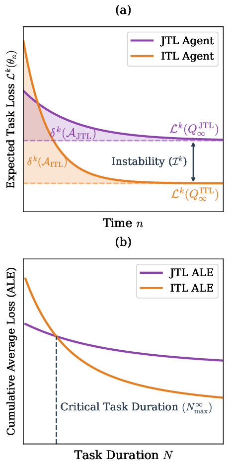
1.0.2.5.1 Pairwise Transfer is Asymmetric, and Why Ordering Matters
To isolate the directional structure of transfer, we measure pairwise interference directly: for every ordered pair \((t_i, t_j)\) of MT10 tasks we train a two-task joint (JTL) agent and compare the performance it achieves on \(t_i\) against the single-task (ITL) specialist for \(t_i\). 20 reports the resulting normalized gap \[\Delta(t_i \mid t_j) \;=\; \frac{\text{ITL}(t_i) - \text{JTL}(t_i \mid t_j)}{\text{ITL}(t_i)},\] where the row indexes the evaluated task \(t_i\) and the column indexes the co-trained task \(t_j\). With the figure’s sign convention, \(\Delta>0\) (red) means joint training (JTL) hurts the row task relative to its ITL specialist (ITL is better), \(\Delta<0\) (blue) means JTL helps it (JTL is better), and the diagonal is \(0\) by construction.
The salient structural fact is that the matrix is not symmetric: in general \(\Delta(t_i \mid t_j) \neq \Delta(t_j \mid t_i)\). Transfer between two tasks is directional—one task can be substantially harmed by a partner that it, in turn, helps. Drawer-close and peg-insert-side, for instance, are improved by joint training with almost every partner (predominantly blue rows), whereas push, pick-place, and button-press-topdown are degraded by most partners (predominantly red rows), and the two directions of a given pair frequently carry opposite signs.
This asymmetry has a direct consequence for the lifelong objective. Because the quantity we ultimately optimize is the time-averaged error across the whole task sequence, a pair in which one direction is positive and the other negative need not produce net-negative transfer: the gains on the helped task can offset or outweigh the losses on the harmed task. More importantly, asymmetry turns task ordering into a usable degree of freedom. Concretely, suppose \(\Delta(t_1 \mid t_2) > 0\) (joint training would hurt \(t_1\)) while \(\Delta(t_2 \mid t_1) < 0\) (joint training helps \(t_2\)). Then presenting the tasks in the order \(t_1 \rightarrow t_2\) (training \(t_1\) alone first, and only introducing \(t_2\) afterwards under joint training) lets \(t_1\) bank its ITL-level performance during its first phase while \(t_2\) reaps the positive transfer during the joint phase. The lifelong error over the pair can then fall below the average of the two ITL specialists, even though the symmetric (simultaneous, from-scratch) joint agent would have shown mixed or negative transfer. In other words, the off-diagonal sign structure of 20 is precisely the lever that the curriculum exploits, and it is the structural reason to adopt an explicit ordering.
We stress that the matrix is measured under simultaneous two-task training from a shared initialization, so it is a proxy for the directional interference. It motivates ordering as a mechanism and explains the observed sensitivity of aggregate TE to the task sequence. A systematic search over orderings that maximize lifelong performance using this asymmetry is a natural direction left to future work.
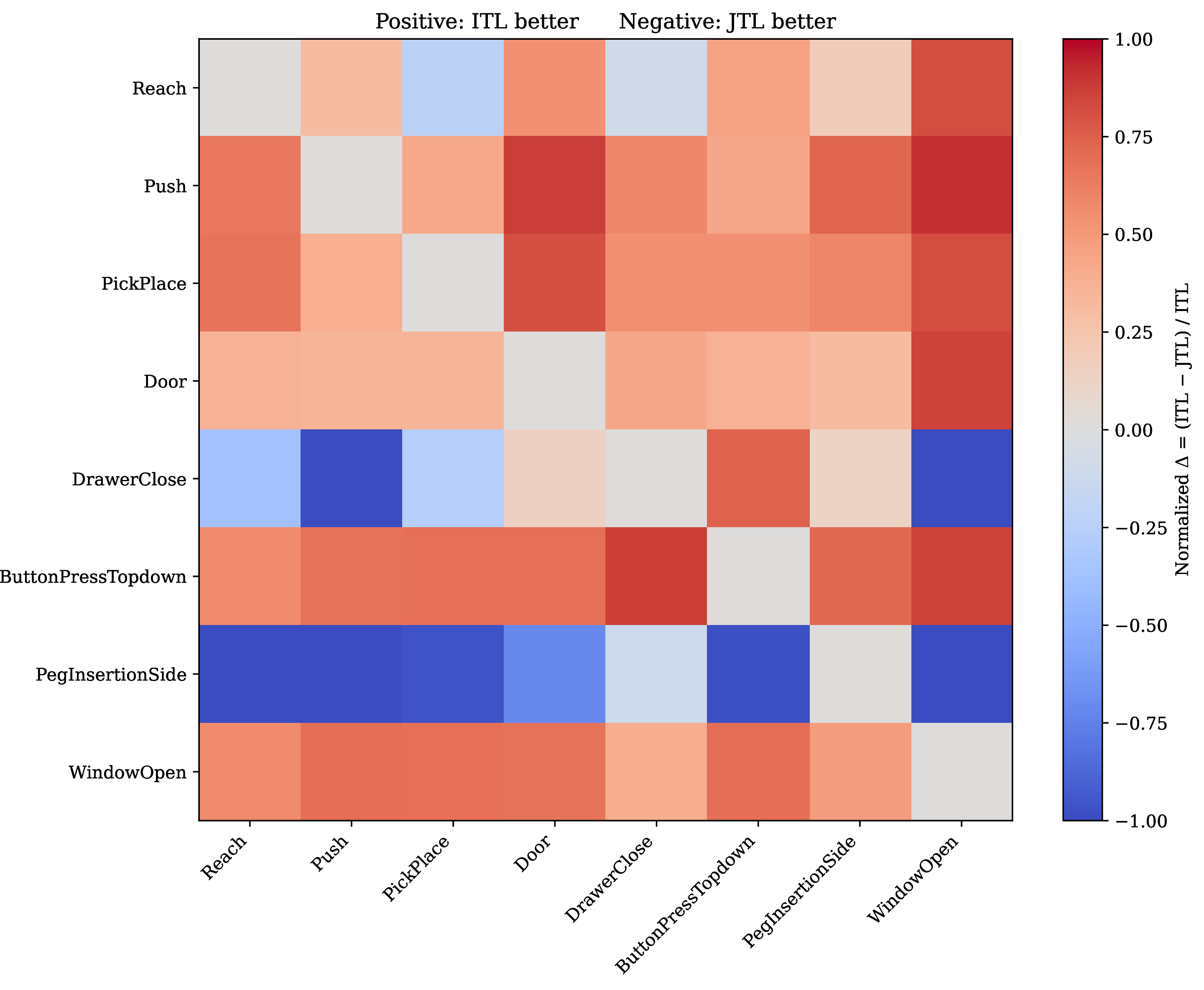
1.0.2.5.2 Proxy measures of instability
We consider two proxies to measure Instability. The first, \(\mathcal{I}_{CU}\), approximates the theoretical definition (3) by training ITL and JTL models to convergence and measuring the difference in their average task-wise error. The second, \(\mathcal{I}_{transfer}\), is a heuristic that measures the average off-diagonal error in a task transfer matrix (i.e., the error of a model trained on task \(i\) when evaluated on task \(j\)). In practice, \(\mathcal{I}_{transfer}\) is computationally cheaper.

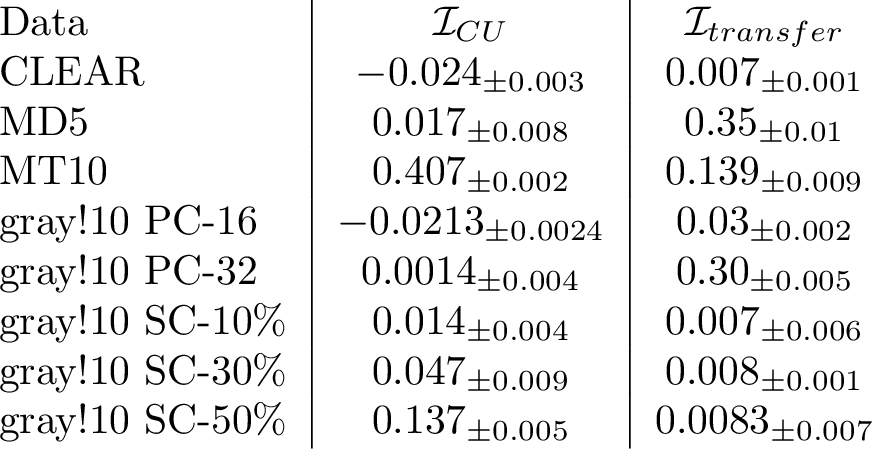
As shown in ¿tbl:tab:instability?, both proxies confirm our qualitative assessment: CLEAR exhibits low Instability, while MD5 and MT10 are high. The proxies also validate our methodology for the controlled benchmarks, showing that Instability increases with the permutation size (PC-16 vs. PC-32) and the label shuffle percentage (SC-10% to SC-50%). The two proxy columns are not expected to match numerically: \(\mathcal{I}_{CU}\) compares the converged JTL and ITL solutions directly, while \(\mathcal{I}_{transfer}\) measures off-diagonal transfer between separately trained task specialists. Their agreement at the level of ordering is the relevant point for our empirical use of Instability.
1.0.2.5.3 Scaling Deep Linear Networks Experiments
Figures 21 and 22 expand the deep-linear study by varying hidden width while holding the data-generating process fixed. These experiments isolate a key message from the optimization-bias analysis: even when the realizable input-output map is linear, the training parametrization changes the TE landscape. Increasing width does not simply make JTL and ITL equivalent. Instead, the lazy and rich regimes trace different families of TE frontiers because they induce different optimization paths, different effective conditioning, and different amounts of Instability after joint training.
The lazy-regime simulations in Figure 21 behave most like the fixed-feature or neural-tangent picture. Width increases capacity and smooths some finite-width effects, but the qualitative transfer boundary remains governed by the same tradeoff as in the shallow theory: JTL reduces transient optimization cost by reusing past data, while it pays an Instability cost when the current task has drifted too far from the historical average. Thus positive TE persists only in regions where the transient savings dominate the mismatch induced by jointly fitting previous tasks.
The rich-regime simulations in Figure 22 show that feature learning changes this balance. Because the representation can move during training, the model is not constrained to interpolate between tasks in the same way as in the lazy regime. This can improve transfer when the tasks share useful structure, but it can also amplify path dependence when the representation learned for earlier tasks is poorly aligned with later ones. The comparison between the two grids therefore supports the claim that TE is not determined only by task drift and sample count; it also depends on the optimizer-induced solution selected within an overparameterized model class.
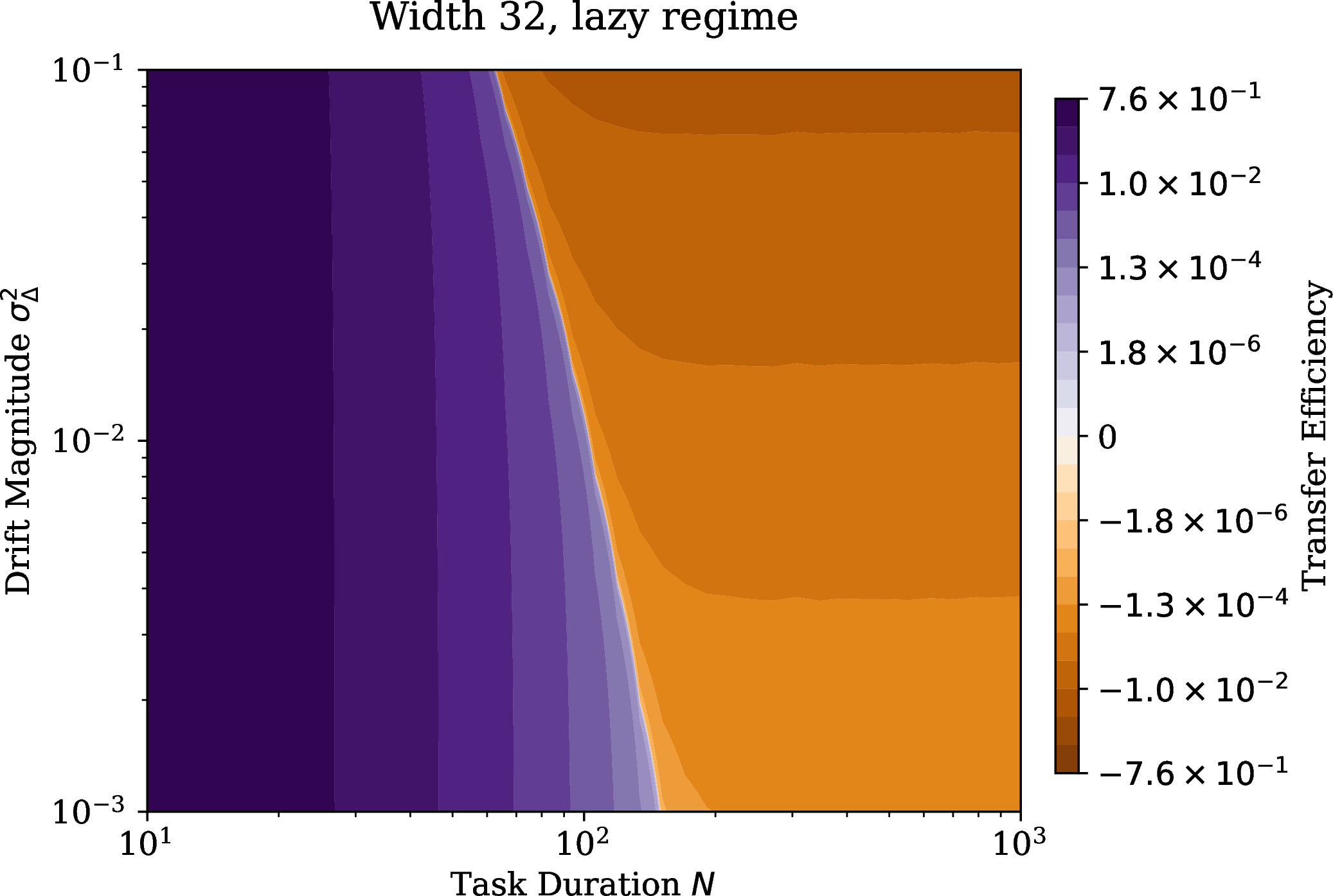
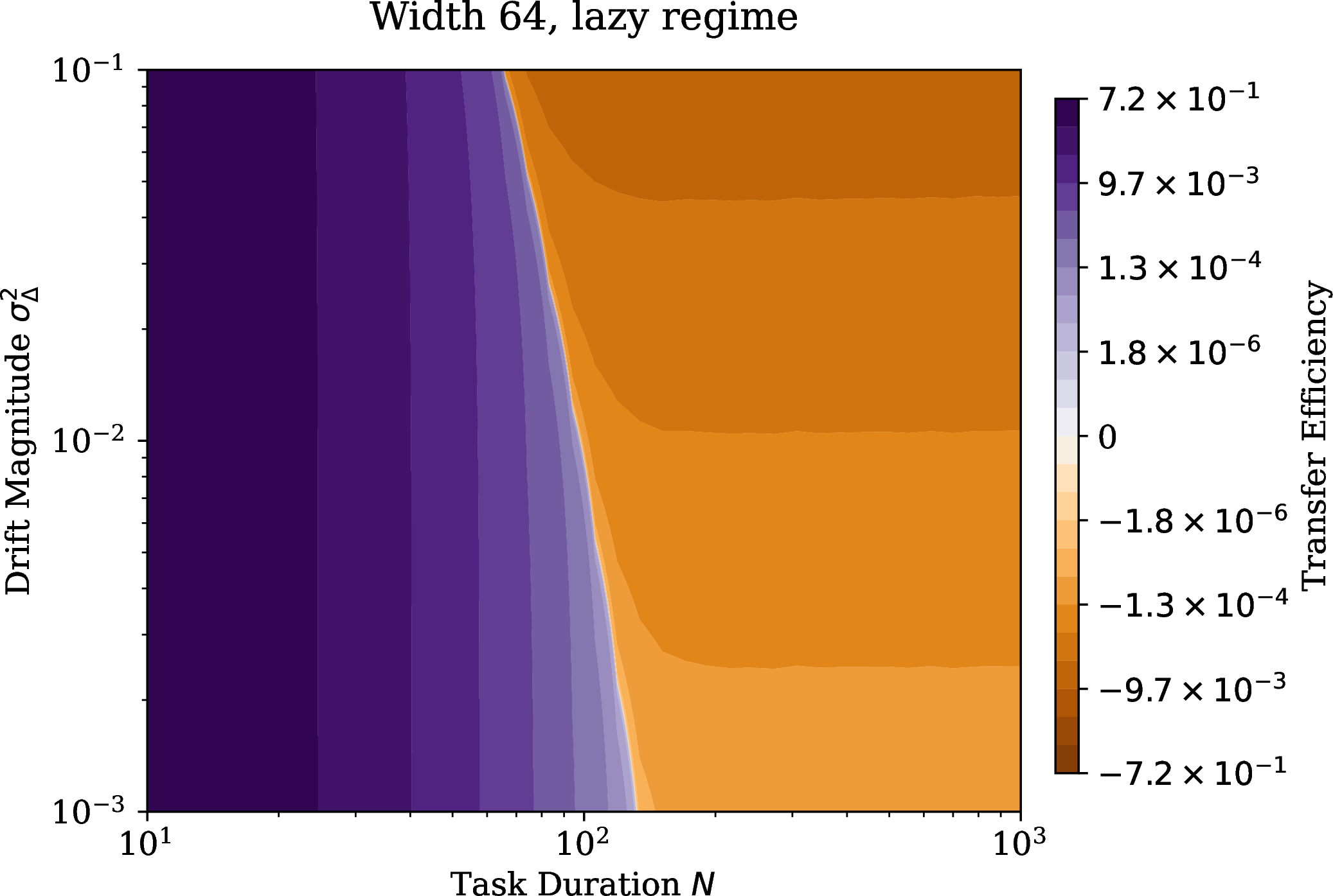
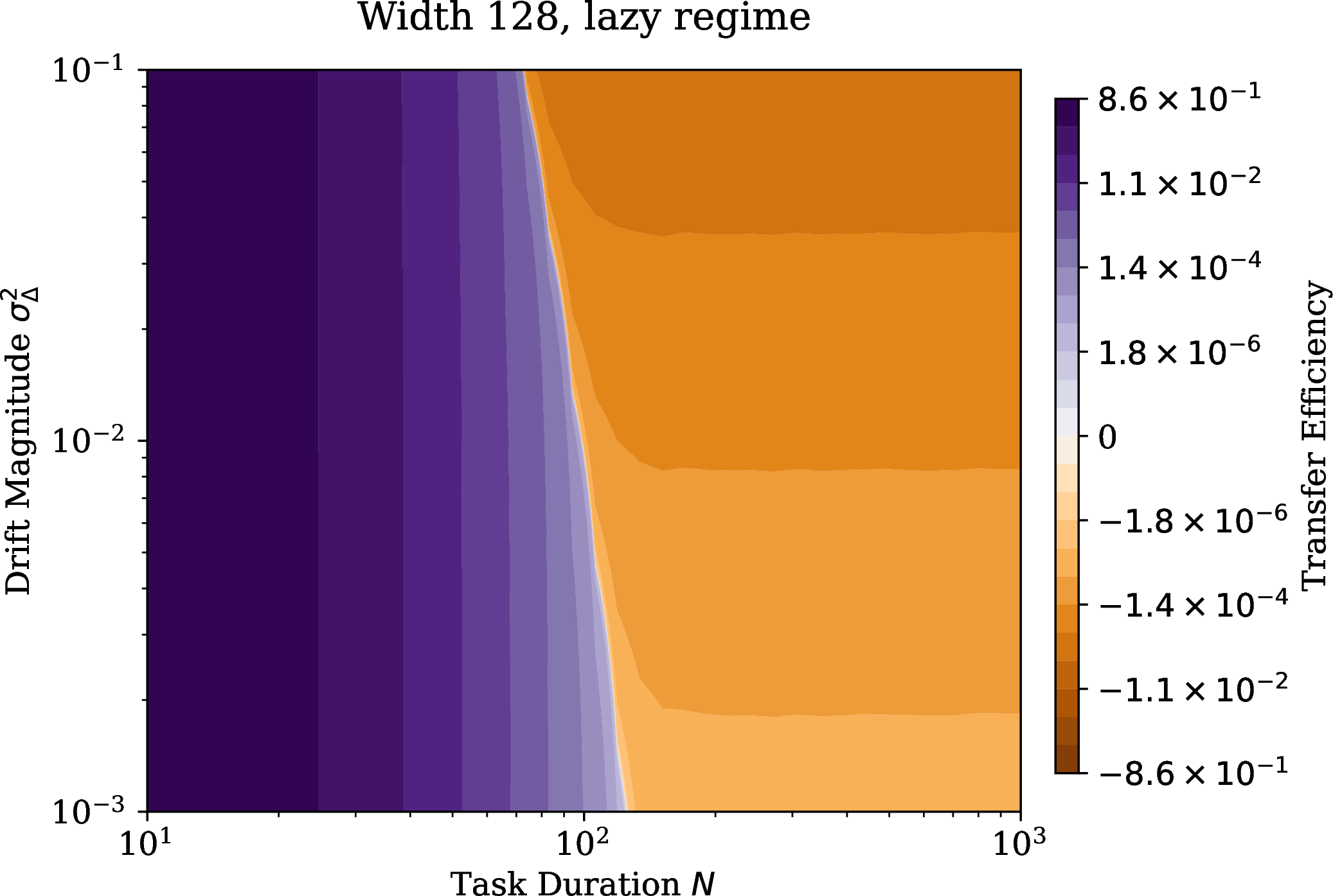
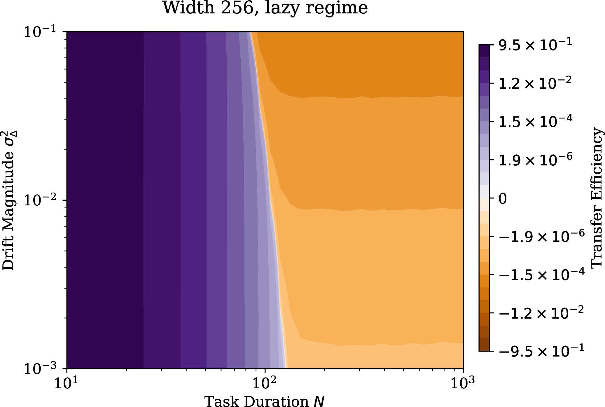
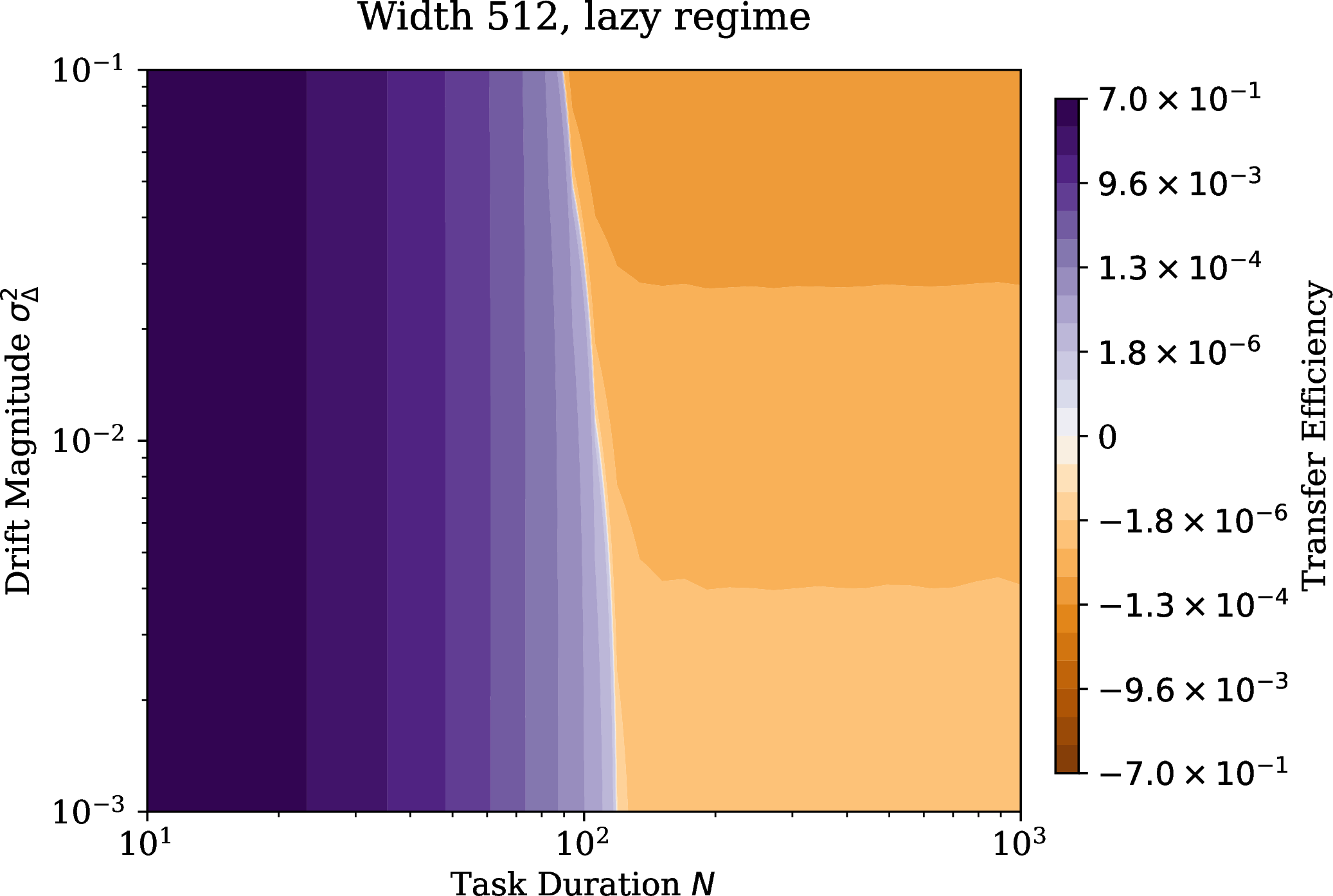
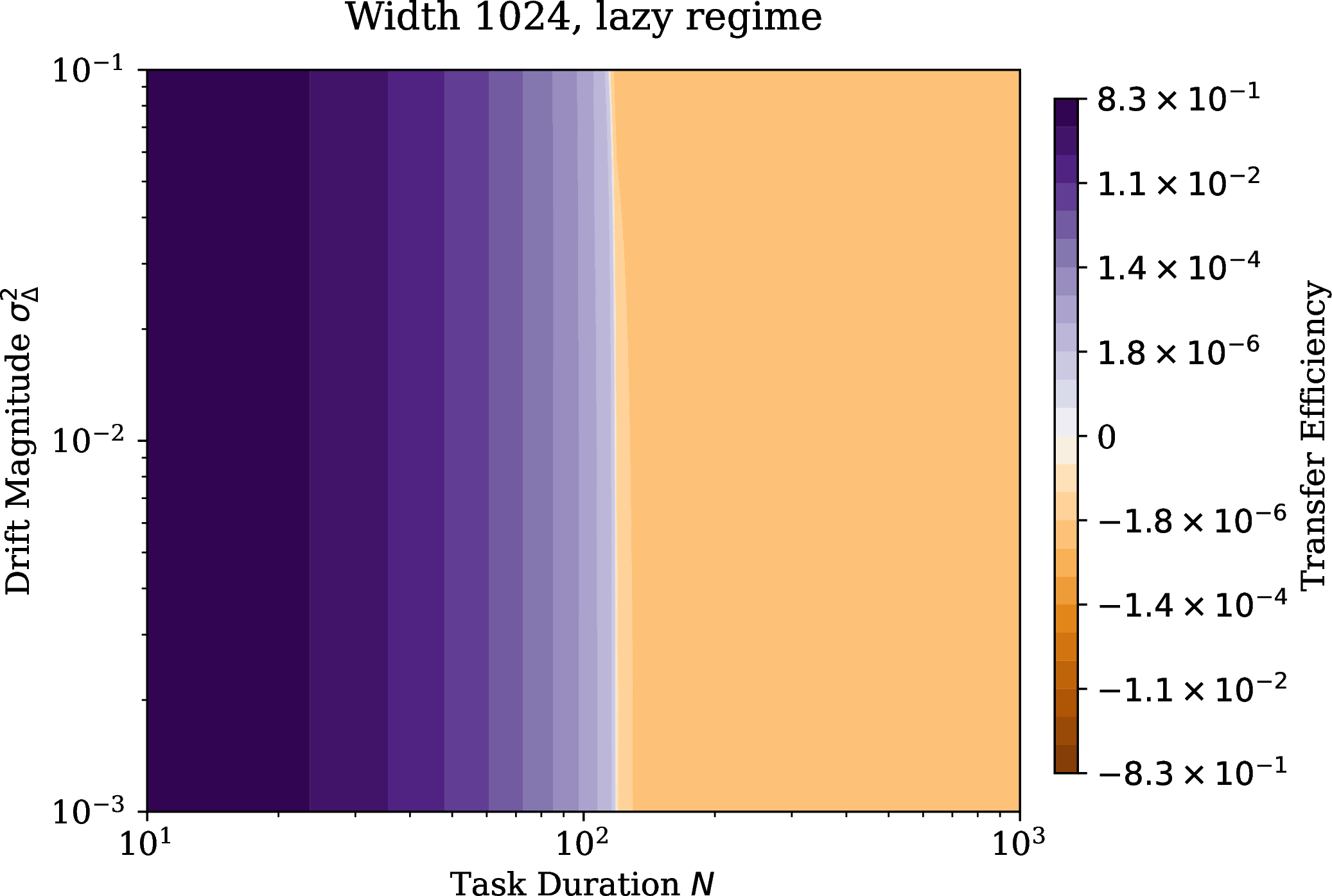
Figure 21: Lazy regime simulations. From left to right the model width is increased from \(32\) to \(1024\) (\(2^5\) folds)..
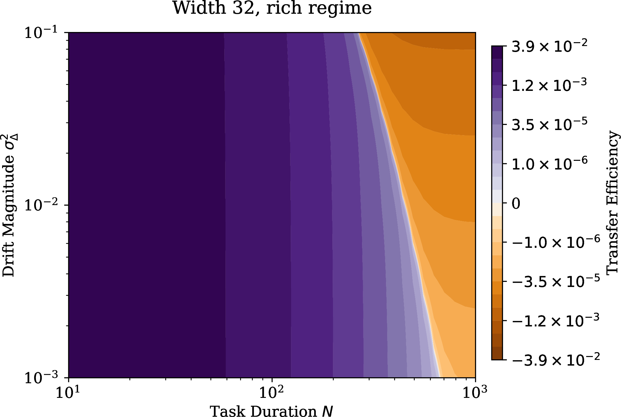
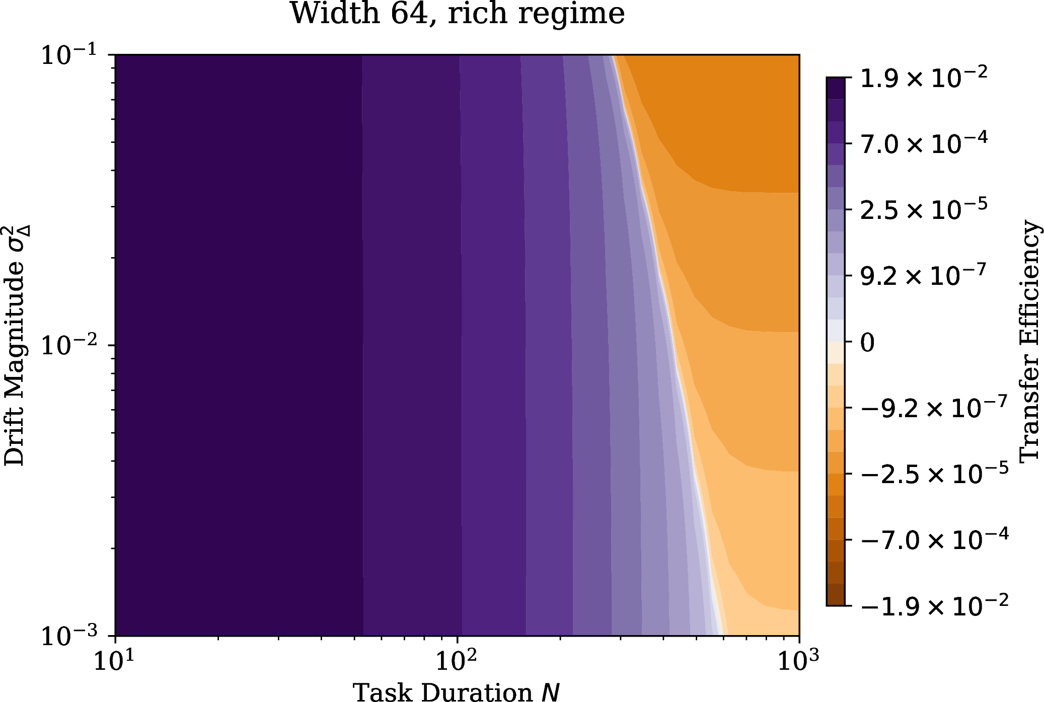
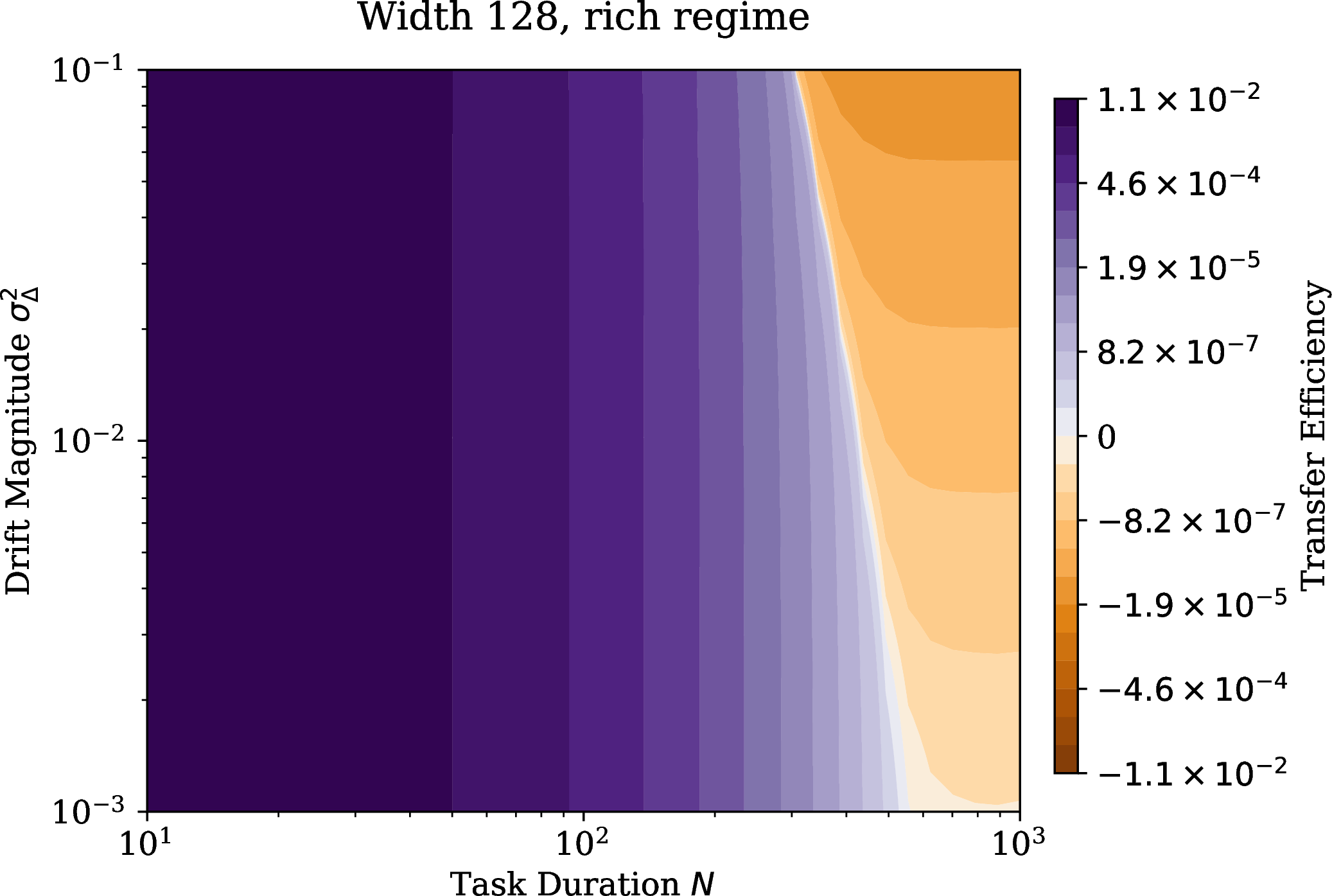

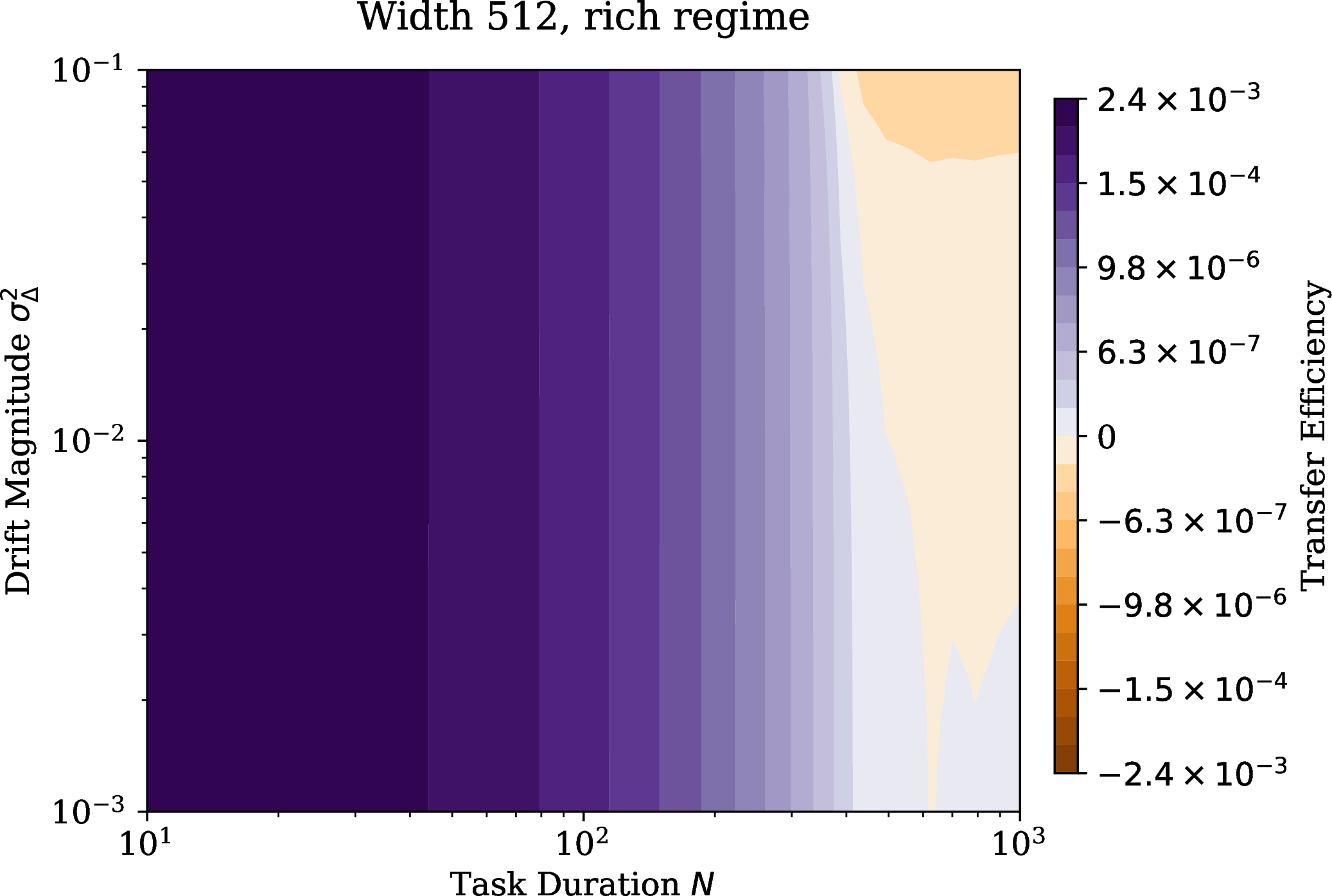
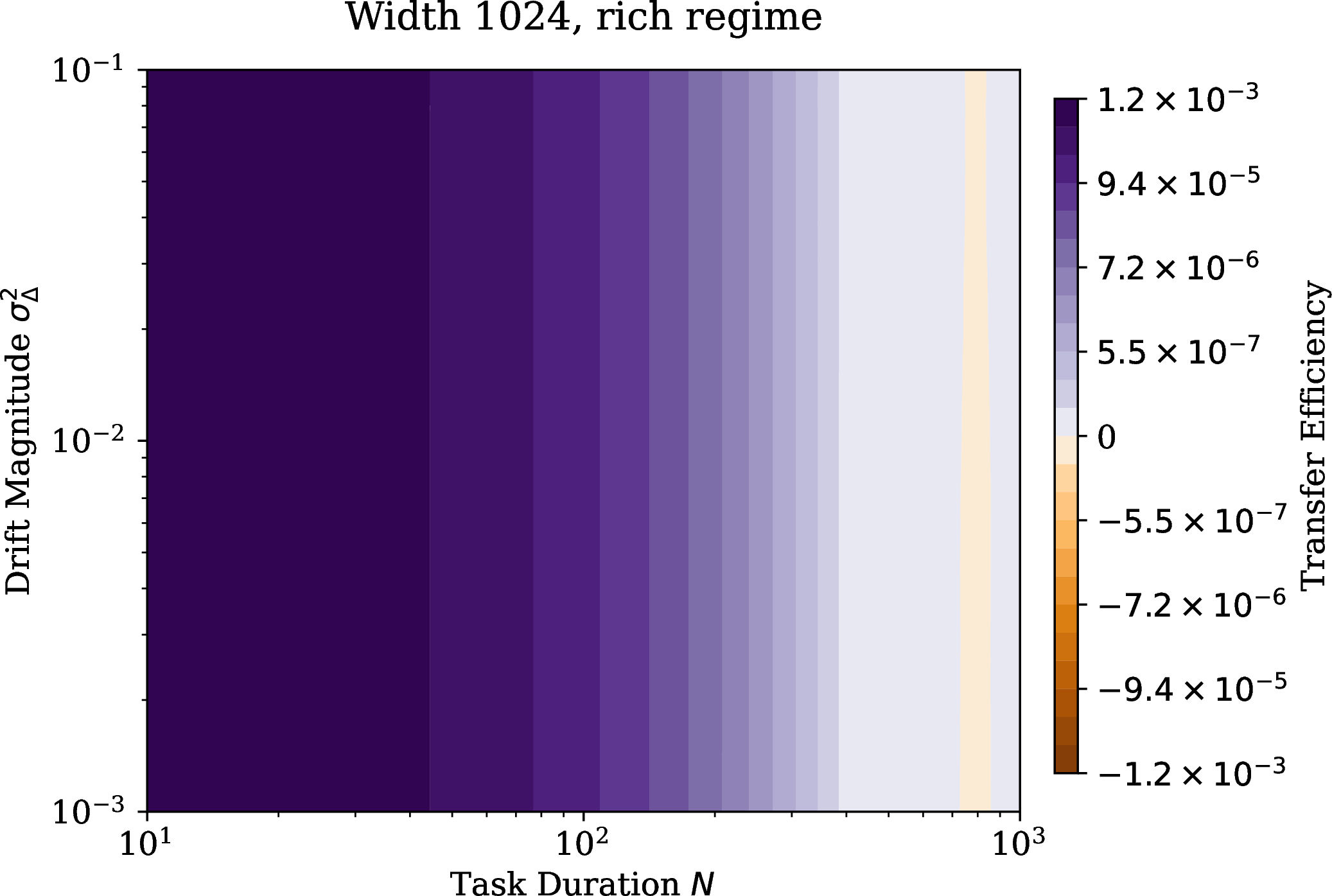
Figure 22: Rich regime simulations. From left to right the model width is increased from \(32\) to \(1024\) (\(2^5\) folds)..

1.0.2.5.4 Real-time training trajectories
The main text reports TE after averaging over tasks and seeds. The trajectories below show where those averages come from in time. In particular, they distinguish transient effects at the beginning of each task from persistent bias or interference accumulated across the sequence.
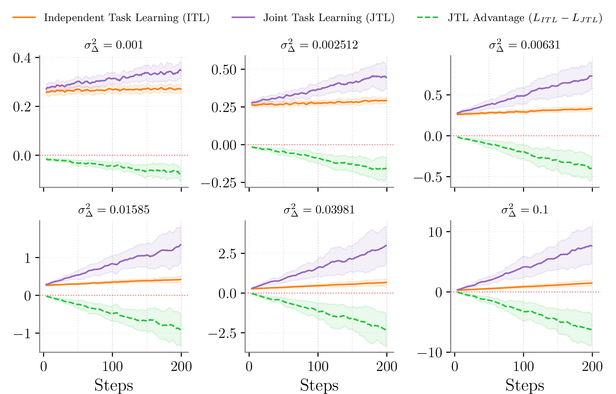
Figure 24 is the trajectory-level analogue of the continuous-drift phase diagrams. At small drift, the history remains predictive of the current optimum, so JTL starts each task closer to a useful solution and the advantage is mostly positive. As drift increases, the same history becomes stale: the transient benefit remains visible near some task changes, but it is eventually outweighed by the stationary error of fitting too many past tasks jointly.
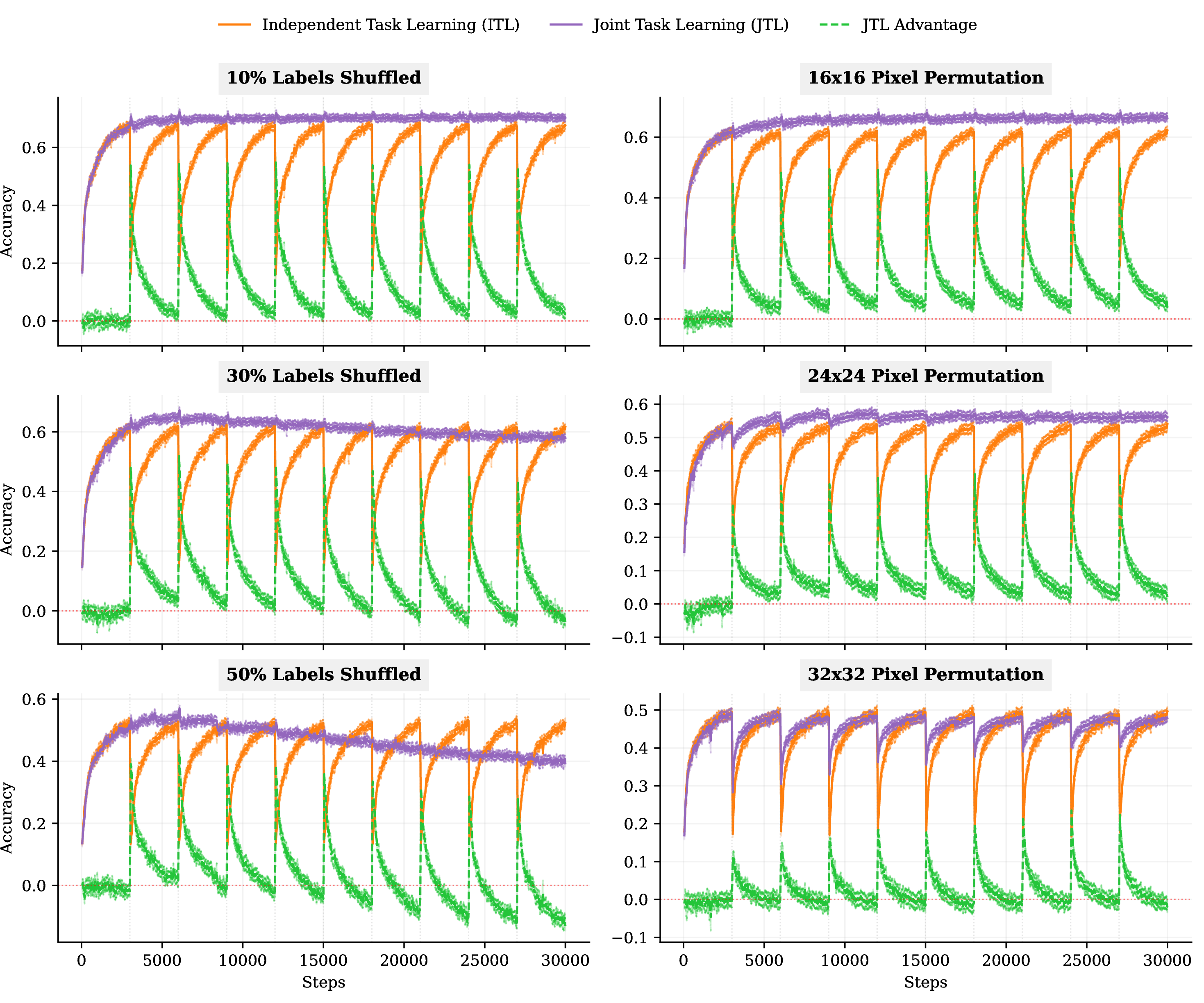
The supervised trajectories in Figure 25 make the same decomposition visible on real benchmarks. CLEAR is the closest empirical analogue of low drift: adjacent tasks share visual and semantic structure, so JTL can reuse previous training. MD5 and the synthetic CIFAR variants create sharper input or label shifts, making the historical data less aligned with the current task and increasing the Instability term.

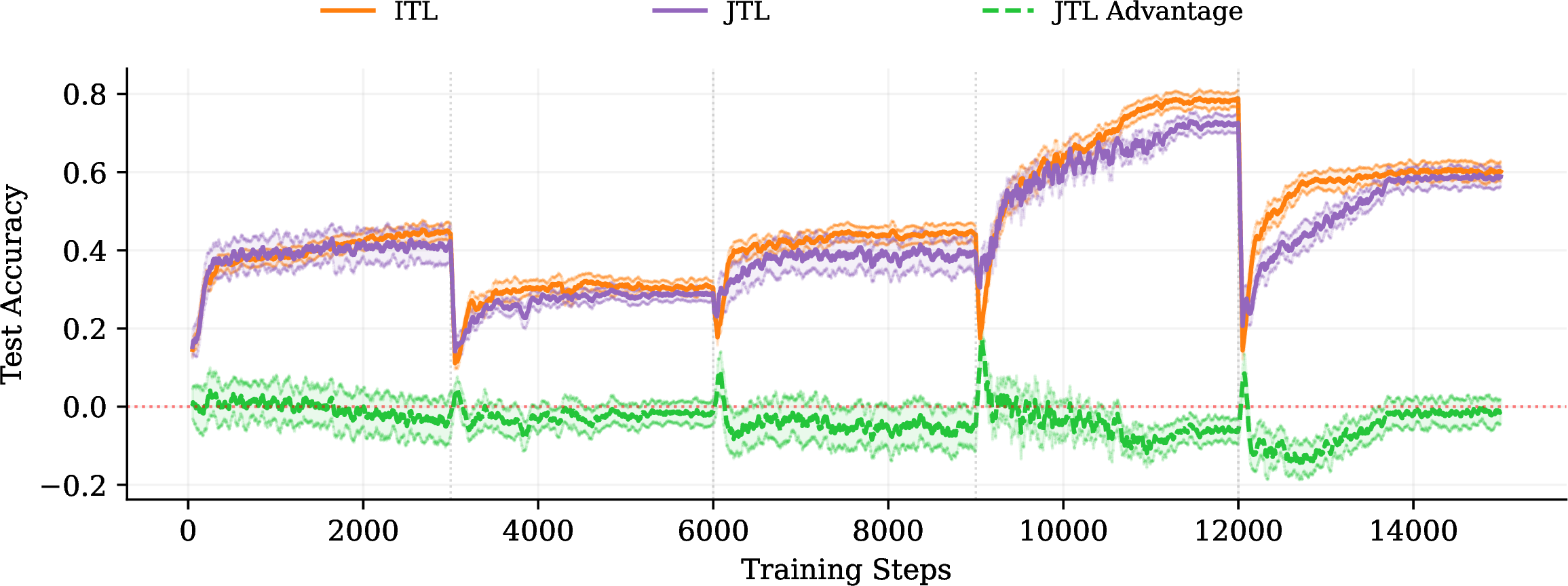
Figure 26: Real-time training dynamics on CLEAR (left) and MD5 (right) at task duration \(N=3000\). Per-task evaluation accuracy of JTL and ITL agents across the full task sequence. The two benchmarks exhibit qualitatively different transfer regimes: smooth temporal drift in CLEAR (where JTL transfer is positive) versus sharp semantic shifts in MD5 (where JTL transfer becomes detrimental)..
Figure 26 highlights the contrast most directly. On CLEAR, the JTL trajectory tends to remain competitive or ahead because the stream changes gradually. On MD5, where each task corresponds to a more abrupt semantic change, JTL is frequently pulled toward earlier classes and ITL benefits from specializing to the current task. This is the empirical counterpart of the sign change in TE as Instability grows.
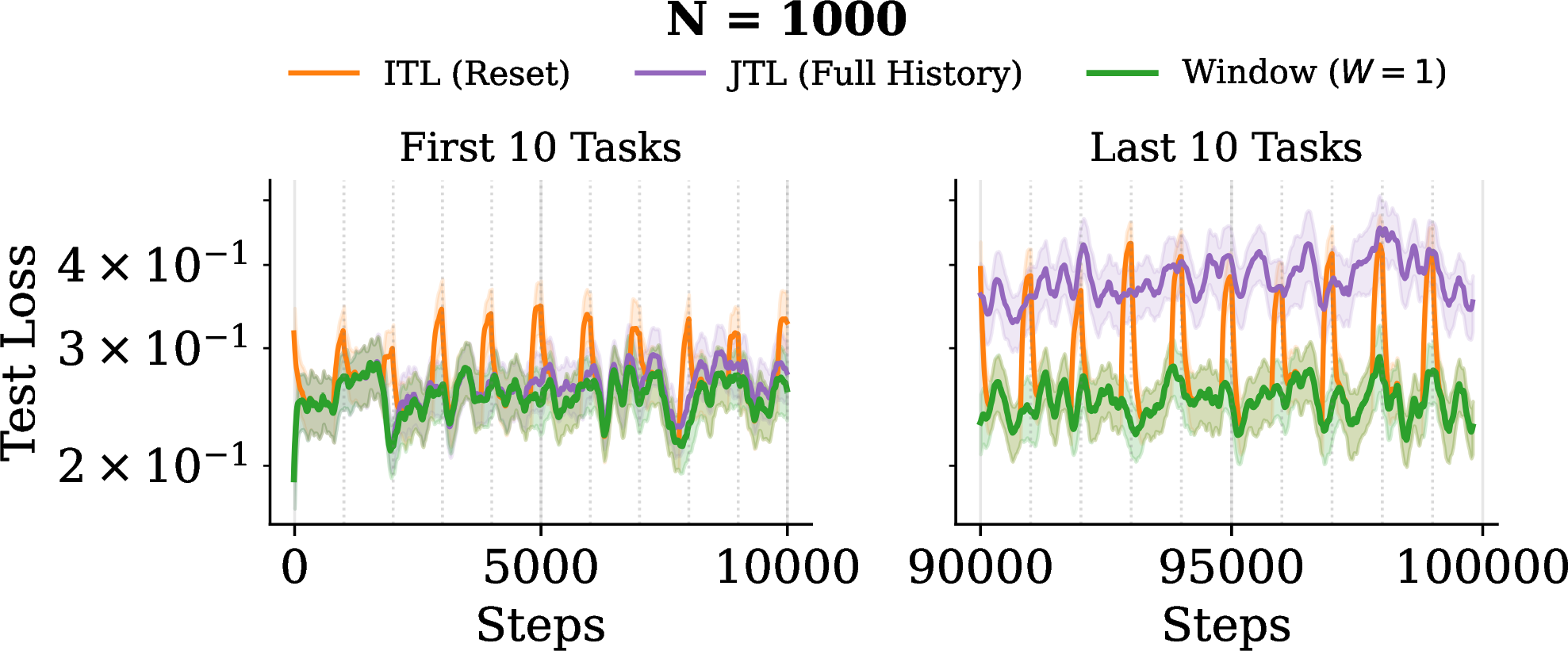
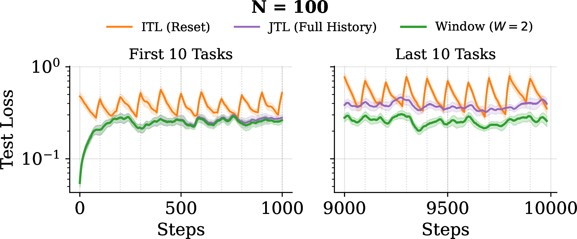
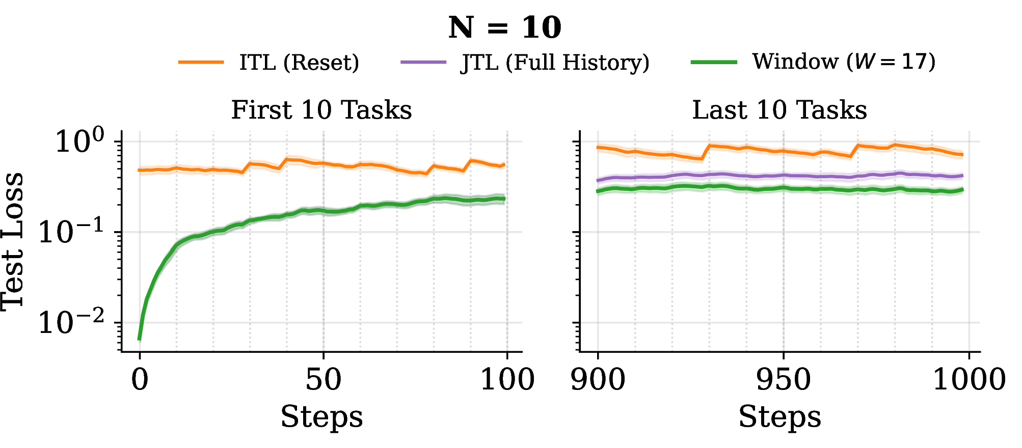
Figure 27: Window-agent trajectory zooms. The first and last ten tasks are shown for several task durations. The window agent keeps only a finite recent history, interpolating between ITL, which uses only the current task, and JTL, which retains the entire stream..
The window-agent zooms in Figure 27 illustrate why a finite memory can outperform both extremes. Early in training, the window and JTL agents are similar because little history exists. Later, the finite window discards obsolete tasks, retaining the transient benefit of recent replay while reducing the bias from distant tasks. This behavior matches the theoretical picture: the best history length grows when tasks are short or drift is slow, and shrinks when old tasks become poor predictors of the current optimum.
References↩︎
Equal contribution.↩︎
Equal supervision.↩︎
We adopt a slightly different notation from the original formulation to better align with the continual learning literature.↩︎
Note that here we’re bypassing the action sampling, which is incorporated in the definition of \(\ell\)↩︎
Hardware optimizations might violate this linear relationship; for the present discussion the linear scaling suffices.↩︎
We use equilibrium, stationary distribution, and convergence point interchangeably throughout the paper. These terms originate in different communities (statistical physics, Markov chains, and optimization respectively), but for the iterate sequence \(\{\theta_n\}\) they all refer to the same object: the limiting distribution \(Q_\infty\) to which \(Q_n\) converges as the algorithm runs on a fixed task. We avoid critical point, which in optimization denotes a zero-gradient parameter value rather than a distribution over parameters.↩︎
In the experiments, expectations under \(Q_n\) and \(Q_\infty\) are estimated empirically: we run multiple training seeds for each algorithm and treat the resulting ensemble of trained models as samples from the parameter distribution at step \(n\). The expected loss \(\mathcal{L}^k(Q_n)\) is then approximated by the average test loss across seeds, and the Instability \(\mathcal{I}^k\) and Transient Error \(\delta^k\) in the decomposition are estimated from this empirical ensemble after the algorithms have converged on each task.↩︎
We assume that \(\mathcal{A}\) has access to the reward function or the history of collected rewards. In supervised learning, this is equivalent to assuming access to the loss function.↩︎
Note that we bypass explicit action sampling here, as it is incorporated into the definition of \(\ell\).↩︎