Abstract Color Voronoi Diagrams and Circular Sequences of Color Permutations
July 06, 2026
Abstract
Abstract Voronoi diagrams are defined in terms of a given system of planar bisecting curves satisfying some simple combinatorial properties. They offer a unifying framework for a wide range of concrete Voronoi instances on generalized sites and metrics. In this paper, we formulate higher-order abstract color Voronoi diagrams of a set \(S\) of \(n\) colored abstract sites, simultaneously considering all concrete instances under their umbrella. We prove that the number of vertices in the order-\(k\) abstract color Voronoi diagram is at most \(4k(n-k)-2n\), and present an iterative construction algorithm. The bound directly applies to a family of \(m\) disjoint simple polygons of total complexity \(n\). For simple polygons the bound can further improve to \(O(\min\{k(n-k),(m-k)^2n\})\). A critical ingredient of our proof is a combinatorial analysis on circular sequences of color permutations derived from the unbounded edges of these diagrams, which is interesting in its own right.
1 Introduction↩︎
Voronoi diagrams are versatile and influential space partitioning structures. Given a set \(S\) of \(n\) sites in \(\mathbb{R}^2\) and an underlying distance function, the ordinary Voronoi diagram \(\mathsf{VD}(S)\) partitions the plane into maximal regions by the nearest site relation. The order-\(k\) Voronoi diagram \(\mathsf{VD}_k(S)\) partitions \(\mathbb{R}^2\) into regions by the \(k\) nearest sites for \(1\leqslant k\leqslant n-1\), where \(\mathsf{VD}_1(S)=\mathsf{VD}(S)\). The farthest-site Voronoi diagram \(\mathsf{FVD}(S)\) is equal to \(\mathsf{VD}_{n-1}(S)\). Sites may often be assumed to be points in the Euclidean plane, however, generalized sites, such as disks, line segments and polygons, under generalized metrics may also constitute the input sites. See [1], [2] for extensive information.
Lee [3] proved the tight bound \(O(k(n-k))\) on the combinatorial complexity of \(\mathsf{VD}_k(S)\) of point sites in the Euclidean plane, and presented an iterative algorithm that computes the diagrams order \(1\) up to \(k\) in \(O(k^2n\log n)\) time. The \(O(k(n-k))\) bound on the complexity of \(\mathsf{VD}_k(S)\) has been extended to line segments under any \(L_p\) metric [4] and to abstract Voronoi diagrams [5]. For point sites in the \(L_1/L_\infty\) metric a better bound \(O(\min\{k(n-k), (n-k)^2\})\) is known [6]. The problem of constructing the Euclidean order-\(k\) Voronoi diagram \(\mathsf{VD}_k(S)\) for point sites \(S\) had been one of the most interesting open problems in computational geometry, and the first optimal \(O(n\log n + k(n-k))\)-time algorithm was presented recently by Chan et al. [7], after a series of algorithmic advances for over four decades [8]–[14]. For generalized sites, however, there is a notable scarcity of corresponding results.
In color Voronoi diagrams, colors are assigned to the sites in \(S\), modeling a common property that sites of the same color share; let \(K\) be the set of these \(m \leqslant n\) colors. The color assignment aggregates simple sites, such as points, segments, or disks, into compound ones of non-constant complexity, such as simple polygons, arc polygons, and site clusters. The color, a non-spatial property, facilitates the modeling of diverse applications, including facility location [15], shape matching [16], spatial databases [17], wireless sensor networks [18], nearest-neighbor classification [19], fault detection and analysis in VLSI networks [20] and references therein. Nearest, higher-order, and farthest color Voronoi diagrams can be naturally defined. Different variants of color Voronoi diagrams have been considered in the literature, such as the Hausdorff (also called cluster) Voronoi diagram, e.g., [20]–[24], and the farthest color Voronoi diagram, e.g., [15], [16], [25], [26], as motivated by different application demands, see e.g., [27], caa?. Higher-order color Voronoi diagrams were recently introduced in [28]. In \(\mathbb{R}^d\), chromatic Delaunay mosaics of colored point sets have also recently been introduced as motivated by topological data analysis [29].
Concrete color Voronoi diagrams are based on distance-to-color functions [28]: for each color \(a \in K\) and any point \(x\in \mathbb{R}^2\), let \(d_a(x) := \min_{s\in S_a} \delta_s(x)\) and \(\bar{d}_a(x) := \max_{s_\in S_a} \delta_s(x)\) be the minimal and maximal distance-to-color \(a\) from \(x\), where \(\delta_s(x)\) denotes the prescribed distance to site \(s\) from \(x\), and \(S_a\subseteq S\) is the set of sites of color \(a\). For each \(1\leqslant k\leqslant m-1\), the order-\(k\) minimal color Voronoi diagram \(\mathsf{CVD}_k(S)\) of colored sites \(S\) partitions \(\mathbb{R}^2\) into regions by \(k\) nearest colors with respect to the minimal distance-to-color functions \(\{d_a\}_{a\in K}\), while the order-\(k\) maximal color Voronoi diagram \(\overline{\mathsf{CVD}}_k(S)\) partitions \(\mathbb{R}^2\) by \(k\) farthest colors with respect to the maximal distance-to-color functions \(\{\bar{d}_a\}_{a\in K}\). In [28] the authors proved the tight upper bound \(4k(n-k)-2n\) on the total number of vertices in \(\mathsf{CVD}_k(S)\) and \(\overline{\mathsf{CVD}}_k(S)\) for a range of well-behaved distance to site functions, under a set of assumptions satisfied by point sites under convex distance functions, and presented an iterative construction algorithm. The assumptions of [28], however, are not satisfied by non-point sites, thus, the derived bounds do not apply in any setting involving sites more general than points. In this paper we remove these assumptions generalizing upon [28].
The order-\(k\) color Voronoi diagrams \(\mathsf{CVD}_k(S)\) and \(\overline{\mathsf{CVD}}_k(S)\) build upon several known diagrams that have received extensive interest in the literature. For \(k=1\), the minimal diagram \(\mathsf{CVD}_1(S)\) is a subset of \(\mathsf{VD}(S)\), while the maximal diagram \(\overline{\mathsf{CVD}}_1(S)\) is contained in \(\mathsf{FVD}(S)\). If \(m=n\), that is, every site in \(S\) has a distinct color, then \(\mathsf{CVD}_k(S)=\mathsf{VD}_k(S)\) and \(\overline{\mathsf{CVD}}_k(S) = \mathsf{VD}_{n-k}(S)\). For \(k=m-1\), \(\mathsf{CVD}_{m{-}1}(S)\) is exactly the farthest color Voronoi diagram \(\mathsf{FCVD}(S)\), and \(\overline{\mathsf{CVD}}_{m-1}(S)\) is the Hausdorff Voronoi diagram \(\mathsf{HVD}(S)\).
Abstract Voronoi diagrams (AVDs) [30] offer a unifying framework for a wide range of concrete Voronoi instances. Rather than sites and distance measures, AVDs are defined in terms of bisecting curves that satisfy some simple combinatorial properties. Examples of concrete diagrams under the AVD umbrella include Voronoi diagrams of (non-intersecting) line segments, or convex polygons of constant complexity, in the \(L_p\) norms; Euclidean Voronoi diagrams of (non-intersecting) disks or smooth convex objects; point sites in any convex distance metric; additively weighted points, and power diagrams, with non-enclosing circles in nice metrics. Bohler et al. [5] proved the tight upper bound \(2k(n-k)+k+1-n\) on the number of faces in the order-\(k\) abstract Voronoi diagram \(\mathsf{VD}_k(S)\). Efficient construction algorithms are also known [31], [32].
Contribution.
In this paper, we formulate higher-order color Voronoi diagrams under the AVD model, namely higher-order abstract color Voronoi diagrams. By using the abstract framework, our combinatorial results are simultaneously applicable to all the concrete instances that fall under the AVD umbrella, which are also interesting individually. The obtained upper bounds are tight and analogous to those in [28], however, they are applicable to a much wider class of problems. This includes the higher-order Voronoi diagram of \(m\) simple polygons whose structural complexity, other than its farthest-site counterpart [33], had been unknown. It also results in the first study on the Hausdorff and farthest color Voronoi diagram in the abstract setting, which encompass all the previously considered concrete cases.
We prove tight upper bounds \(O(k(n-k))\) on the combinatorial complexity of order-\(k\) abstract color Voronoi diagrams \(\mathsf{CVD}_k(S)\) and \(\overline{\mathsf{CVD}}_k(S)\) for each \(1\leqslant k\leqslant m-1\). More precisely, we show that the number of vertices of the abstract \(\mathsf{CVD}_k(S)\) and \(\overline{\mathsf{CVD}}_k(S)\) is at most \(4k(n-k)-2n\), which is tight. This immediately implies the worst-case bound \(O(m(n-m+1))\) on the complexity of the abstract farthest color Voronoi diagram \(\mathsf{FCVD}(S)\) and the abstract Hausdorff Voronoi diagram \(\mathsf{HVD}(S)\), which applies to all the concrete cases under the AVD umbrella. If \(m\) is close to \(n\), then our new bound improves the previous one \((O(mn))\) on the complexity of the farthest color Voronoi diagram of non-crossing line segments in the \(L_p\) metric [16], [25]. For a family of \(m\) disjoint simple polygons of total complexity \(n\), we show that the order-\(k\) polygon Voronoi diagram has complexity \(O(\min\{k(n-k),(m-k)^2n\})\). This is derived from a more general result: if the farthest color Voronoi diagram \(\mathsf{FCVD}(S')\) (resp. \(\mathsf{HVD}(S')\)) for any subset \(S'\subseteq S\) has linear complexity, then \(\mathsf{CVD}_{k}(S)\) (resp. \(\overline{\mathsf{CVD}}_{k}(S)\)) has complexity \(O((m-k)^2 n)\) for \(\frac{2m}{3} \leqslant k\leqslant m-1\). Note that the farthest polygon Voronoi diagram has linear complexity [33]. The complexity of the order-\(k\) Voronoi diagram of polygons had been an open problem for a long time.
To obtain these results we first adapt the colorful Clarkson–Shor technique from [28], [34] to abstract Voronoi diagrams, expressing the combinatorial complexity of the order-\(k\) abstract color Voronoi diagram as a function of the diagram’s unbounded edges (see Lemma [lem:complexity]). This reduces the problem into counting the unbounded edges of the colored order-\(k\) diagrams. For \(m=n\) (uncolored case) this already answers a question posed by the authors of [5] on whether the Clarkson–Shor technique [34] could be applied in deriving the complexity of the abstract order-\(k\) diagram. Deriving bounds on the unbounded edges of colored order-\(k\) diagrams is a critical part of our proof, which is a novel contribution of this paper. In [28] the involved quantities were assumed equal and these bounds could thus be bypassed, which is valid for point sites in convex metrics, but does not extend to more general cases.
An independently interesting ingredient of our combinatorial results is based on a circular sequence of permutations of colored elements, which correspond to the unbounded edges of the diagrams. Circular sequences of permutations, sometimes called allowable sequences, have been useful as a purely combinatorial tool to analyze several basic geometric structures such as \(k\)-sets and order types [35]–[37]. We consider a colored variant of circular sequences, in which each element of permutations is assigned a color, and prove tight lower and upper bounds on the number of switches, which reflect the unbounded edges of order-\(k\) abstract color Voronoi diagrams.
Finally, we show how to construct both \(\mathsf{CVD}_k(S)\) and \(\overline{\mathsf{CVD}}_k(S)\) in an iterative fashion, for orders \(1\) to \(k\), in time \(O(k^2n\log n)\). Because \(\overline{\mathsf{CVD}}_{k-1}(S)\) does not contain sufficient information to compute \(\overline{\mathsf{CVD}}_k(S)\), we first provide a direct divide-and-conquer algorithm to compute the unbounded edges of \(\overline{\mathsf{CVD}}_{k}(S)\) in time \(O(k^2(n-k) \log m + n \log n)\), after which \(\overline{\mathsf{CVD}}_k(S)\) can be computed from \(\overline{\mathsf{CVD}}_{k-1}(S)\). A byproduct of this technique leads to an \(O((n-k)^2n\log n)\)-time iterative algorithm to compute the (uncolored) order-\(k\) abstract Voronoi diagram \(\mathsf{VD}_k(S)\), in decreasing order of \(k\), starting from \(\mathsf{FVD}(S)\), which is efficient for large values of \(k\). To the best of our knowledge, no such algorithm was known before.
2 Review on higher-order abstract Voronoi diagrams↩︎
For any \(A \subseteq \mathbb{R}^2\), we denote by \(\mathop{\partial}A\), \(\mathop{\mathrm{int}}A\), and \(\mathop{\mathrm{cl}}A\) the boundary, interior, and closure of \(A\), respectively.
Let \(S\) be a set of \(n\) abstract sites that define a family \(\mathcal{J}= \{J({p},{q}) \mid p,q\in S, p\neq q\}\) of bisecting curves. The bisector \(J({p},{q})\) of two sites \(p,q\in S\) is an unbounded simple curve, homeomorphic to a line, that divides the plane into two open domains: the dominance region of \(p\) over \(q\) and the dominance region of \(q\) over \(p\), denoted by \(D({p},{q})\) and \(D({q},{p})\), respectively, see [30]. The dominance region \(D({p},{q})\) can be regarded as the set of all points that are nearer to \(p\) than to \(q\) according to a relevant proximity notion.
The nearest and the farthest Voronoi region of site \(p\in S\) are respectively defined as \(\mathrm{VR}(p, S) := \bigcap_{q \in S \setminus \{p\}} D({p},{q}) \quad\text{and}\quad \mathrm{FVR}(p, S) := \bigcap_{q\in S\setminus\{p\}} D({q},{p}).\) The nearest Voronoi diagram \(\mathsf{VD}(S)\) and the farthest Voronoi diagram \(\mathsf{FVD}(S)\) are the collection of the region boundaries: \(\mathsf{VD}(S) := \bigcup_{p\in S} \mathop{\partial}\mathrm{VR}(p, S) \quad\text{and}\quad \mathsf{FVD}(S) := \bigcup_{p\in S} \mathop{\partial}\mathrm{FVR}(p,S).\)
The family of bisecting curves \(\mathcal{J}\) is called admissible if it satisfies the following axioms [30], for every \(S'\subseteq S\):
Each nearest Voronoi region \(\mathrm{VR}(p, S')\) is non-empty and pathwise connected.
Each point of the plane belongs to the closure of a nearest Voronoi region \(\mathrm{VR}(p, S')\).
Each bisector \(J({p},{q})\) is unbounded. After stereographic projection to the sphere, it can be completed to a closed Jordan curve through the north pole.
Any two bisectors intersect transversally, in a finite number of points.
Axiom (A4) can be relaxed as shown in [38] but for technical simplicity we still require it. The verification of the axioms can be done with constant size (\(\leqslant 4\)) examples, see [5]. Bisectors that have a site in common are called related. When two related bisectors \(J({p},{q})\) and \(J({p},{r})\) intersect, bisector \(J({q},{r})\) intersects with them at the same point(s). If \(\mathcal{J}\) is admissible, there are at most two such intersection points, which are the vertices of \(\mathsf{VD}(\{p,q,r\})\). Then \(\mathsf{VD}(S)\) and \(\mathsf{FVD}(S)\) are plane graphs of complexity \(O(n)\) [30], and \(\mathsf{FVD}(S)\) is a tree [39].
The higher-order abstract Voronoi diagram was first introduced in [5]. For \(1\leqslant k\leqslant n-1\) and each subset \(H \subset S\) with cardinality \(k\), the order-\(k\) Voronoi region of \(H\) and the order-\(k\) abstract Voronoi diagram \(\mathsf{VD}_k(S)\) are defined as \[\mathrm{VR}_k(H,S) := \bigcap_{p \in H, q \in S \setminus H} D({p},{q}) \quad\text{and}\quad \mathsf{VD}_k(S) := \bigcup_{H\subseteq S, |H|=k} \mathop{\partial}\mathrm{VR}_k(H, S).\] Note that \(\mathsf{VD}_1(S) = \mathsf{VD}(S)\) and \(\mathsf{VD}_{n-1}(S) = \mathsf{FVD}(S)\). The higher-order abstract Voronoi diagram \(\mathsf{VD}_k(S)\) is a plane graph that encompasses classic concrete cases, including points [3] and segments [4] in the Euclidean plane, from which the tight combinatorial complexity bound \(O(k(n-k))\) is also derived [5].
The dominance regions define an abstract notion of \(k\)-th nearest site. In particular, given \(\mathcal{J}\) and a point \(x\in\mathbb{R}^2\), a total order of \(S\) can be defined [5], [31]. For \(p,q\in S\), we write \[p <_x q~\text{iff}~p\neq q~\text{and}~x \in D({p},{q}), \; p =_x q~\text{iff}~p = q~\text{or}~x \in J({p},{q}), \;p \leqslant_x q~\text{iff}~p<_x q~\text{or}~p =_x q.\] These relations can be interpreted as \(x\) being nearer to \(p\) than to \(q\), equidistant to \(p\) and \(q\), and not farther from \(p\) than from \(q\), respectively. The axioms imply the transitivity of \(<_x\) [30] and its reflexive closure \(\leqslant_x\) [31], which define a total order on \(S\) allowing us to say that \(p_k\) is the \(k\)-th nearest site at \(x\). In this sense, the order-\(k\) region \(\mathrm{VR}_k(H, S)\) of \(H\subseteq S\) consists of all points \(x\) such that \(H\) is the set of \(k\) nearest sites at \(x\).
Let \(\Gamma\) be a closed simple curve in \(\mathbb{R}^2\) sufficiently large such that no pair of bisecting curves in \(\mathcal{J}\) cross on or outside of \(\Gamma\); furthermore, every bisecting curve intersects \(\Gamma\) transversally, exactly twice. By this construction, \(\Gamma\) encloses every vertex of \(\mathsf{VD}_k(S)\), for \(1\leqslant k\leqslant n-1\), and the unbounded features of \(\mathsf{VD}_k(S)\) are traversed by \(\Gamma\) in the same order as they appear at infinity. We consider \(\Gamma\) as the closed curve at infinity.
An admissible bisector system \(\mathcal{J}\) is said to be in general position, if only three related bisecting curves can intersect at the same point. From now on, we assume that the given system \(\mathcal{J}\) of bisecting curves is admissible and in general position.
Circular sequences of permutations.
The authors of [5] proved that the number of faces in the order-\(k\) diagram \(\mathsf{VD}_k(S)\) is at most \(2k(n{-}k){+}k{+}1{-}n\) and at least \(n-k+1\). Their combinatorial result is based on an inductive approach extending the original method by Lee [3], which had been extended to segment sites in [4], and a careful analysis on the circular sequences induced by the unbounded edges of \(\mathsf{VD}_k(S)\), for all orders \(1\leqslant k \leqslant n-1\), on the closed curve \(\Gamma\) at infinity.
For each \(x\in \Gamma\), consider the permutation \(\pi=(p_1, \ldots, p_n)\) of \(S\) induced by \(\leqslant_x\). If \(x\) avoids all bisecting curves in \(\mathcal{J}\), then \(\leqslant_x\) induces a unique permutation \((p_1, \ldots, p_n)\) such that \(p_1 <_x \cdots <_x p_n\); otherwise, there is a unique index \(j\) such that \(x \in J({p_j},{p_{j+1}})\) and hence \(p_1<_x \cdots <_x p_j =_x p_{j+1} <_x \cdots <_x p_n.\) The corresponding permutation of \(S\) changes by a switch of two consecutive sites when and only when we cross a bisector \(J({p},{q})\), while we walk along \(\Gamma\). As a result, we obtain a circular sequence \(\Pi(S) = (\pi_0, \ldots, \pi_{N-1}, \pi_N = \pi_0)\) of permutations \(\pi_i\) of sites \(S\) such that:
(P1)
\(\pi_i\) and \(\pi_{i+1}\) for any \(i\) differ by a switch of two consecutive elements; and
(P2)
each pair of two elements switches exactly twice. (\(N=2\binom{n}{2}=n(n-1)\)).
In [5] the authors showed that each switch between positions \(k\) and \(k+1\) in \(\pi_i\) and \(\pi_{i+1}\) corresponds to an unbounded edge of \(\mathsf{VD}_k(S)\). Thus, they obtained tight lower and upper bounds on the total number of unbounded edges in the diagrams \(\mathsf{VD}_1(S), \ldots, \mathsf{VD}_k(S)\) by proving tight bounds on the number of switches in the first \(k\) positions: at least \(k(k+1)\) and at most \(k(2n-k-1)\).
3 Defining abstract color Voronoi diagrams↩︎
Let \(S\) be a set of \(n\) sites and \(\mathcal{J}= \{J({p},{q}) \mid p,q\in S, p\neq q\}\) be an admissible bisector system in general position. We assume that each site \(p\in S\) is assigned a color from a set \(K = \{1, \ldots, m\}\) of \(m\leqslant n\) colors. Let \(S_a \subseteq S\) be the set of sites of color \(a \in K\).
Abstract color Voronoi diagrams can be seen as Voronoi diagrams of colors in \(K\), where each color \(a\in K\) represents its entire color class \(S_a\). We consider two kinds of color dominance regions: for each pair of two distinct colors \(a,b\in K\), define \[D({a},{b}) := \mathop{\mathrm{int}}\left( \bigcup_{p \in S_a} \mathop{\mathrm{cl}}\mathrm{VR}(p, S_a\cup S_b) \right) \quad\text{and}\quad \overline{D}({a},{b}) := \mathop{\mathrm{int}}\left( \bigcup_{p \in S_a} \mathop{\mathrm{cl}}\mathrm{FVR}(p, S_a\cup S_b) \right)\] called the minimal and maximal color dominance regions of color \(a\) over color \(b\), respectively. See the red and blue regions in Figure 1.
Let \(J({a},{b}) := \mathop{\partial}D({a},{b})\) and \(\overline{J}({a},{b}) := \mathop{\partial}\overline{D}({a},{b})\) be the minimal and maximal color bisector, respectively, between two colors \(a,b\in K\). Since \(J({a},{b})\) (resp. \(\overline{J}({a},{b})\)) separates Voronoi regions of different color in \(\mathsf{VD}(S_a\cup S_b)\) (resp. \(\mathsf{FVD}(S_a\cup S_b)\)), it may consist of several disjoint simple curves, either unbounded or closed; see Figure 1. In particular, the minimal bisector \(J({a},{b})\) consists of one or more unbounded or closed curves, while the maximal bisector \(\overline{J}({a},{b})\) consists of only unbounded curves and can also be an empty set. These color bisectors may contain degree-\(2\) vertices.
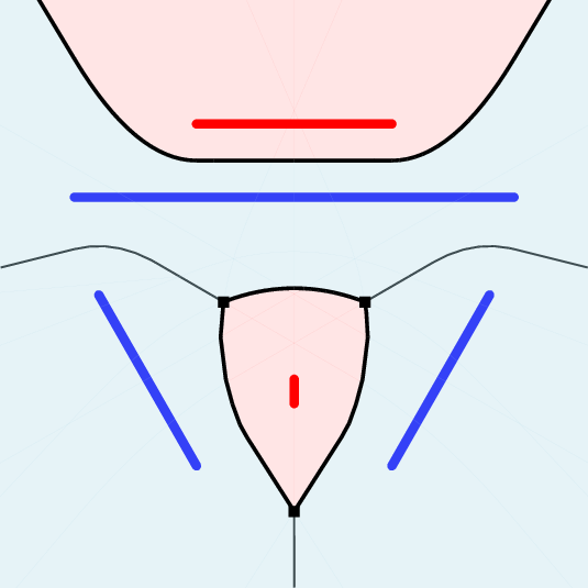
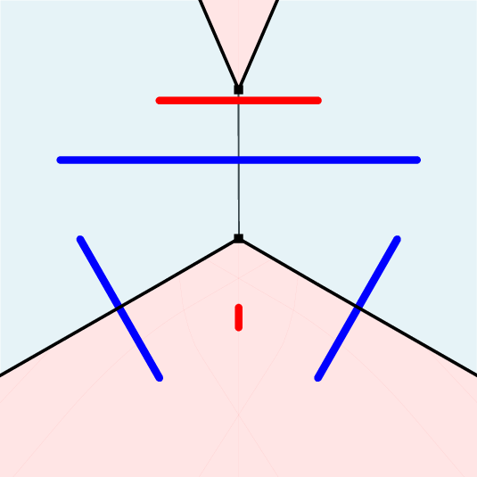
Figure 1: Minimal and maximal dominance regions. The red segments are \(S_a\) and the blue ones are \(S_b\). The thin edges belong to \(\mathsf{VD}(S_a\cup S_b)\) and \(\mathsf{FVD}(S_a\cup S_b)\), the color bisectors are in bold..
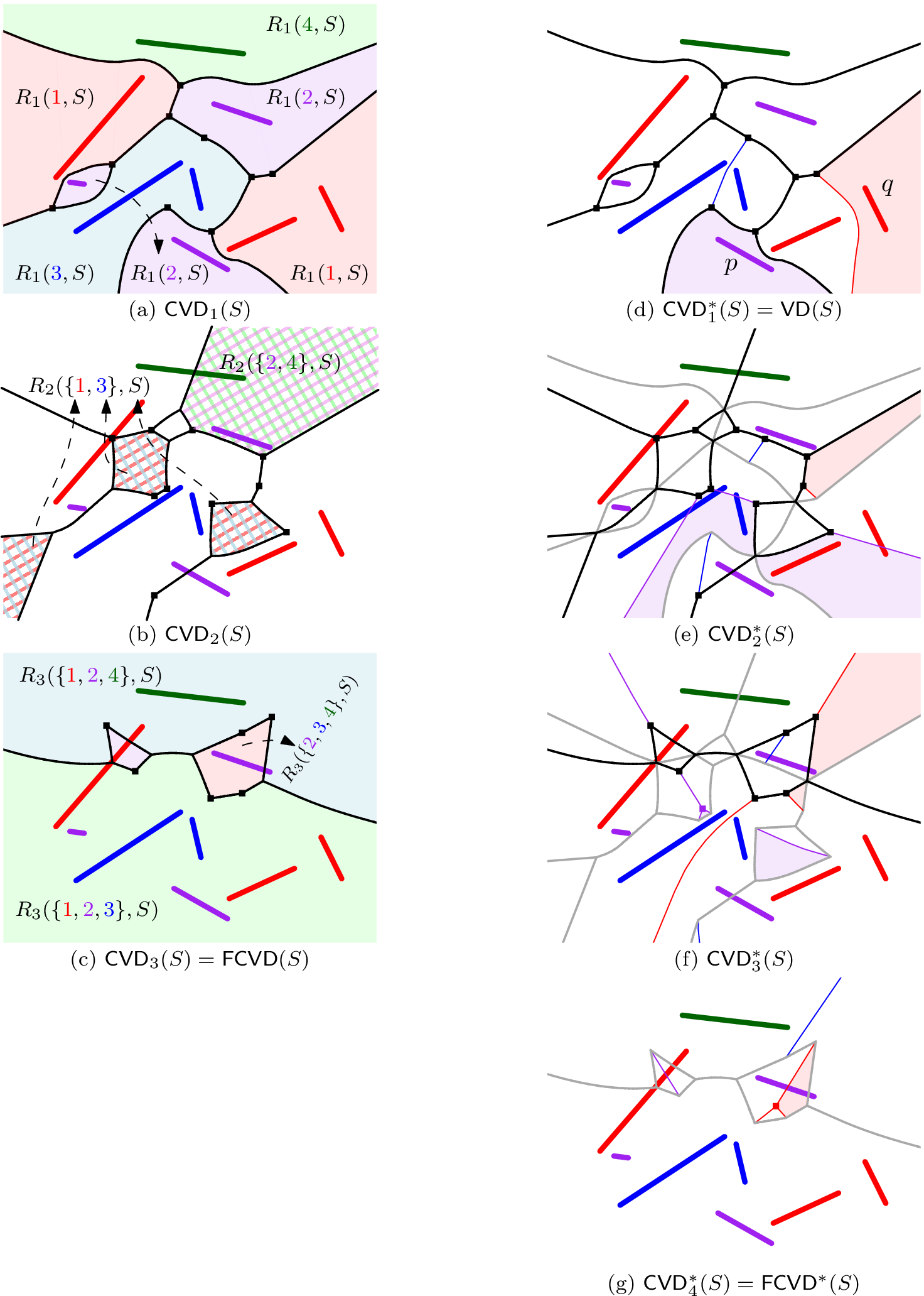
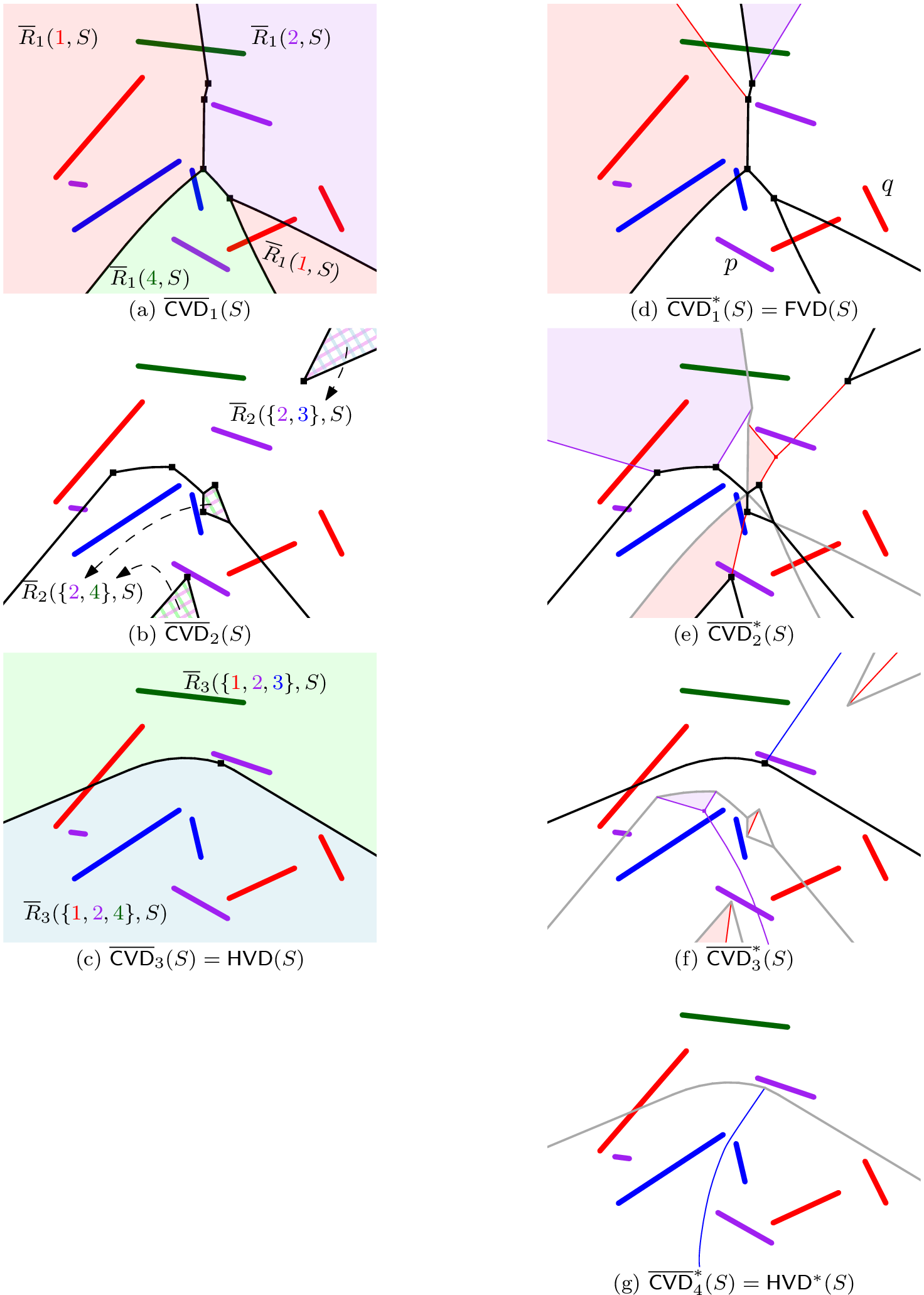
The two kinds of color dominance regions define two hierarchies of higher-order abstract color Voronoi diagrams; see Figures 3 (a–c) and 4 (a–c). For each subset \(H\subseteq K\) of \(k\) colors, the order-\(k\) minimal and maximal color Voronoi regions are defined as \[\mathrm{R}_k(H,S) := \bigcap_{a \in H, b \in K \setminus H} D({a},{b}) \quad\quad \text{and} \quad\quad \overline{\mathrm{R}}_k(H,S) := \bigcap_{a \in H, b \in K \setminus H} \overline{D}({a},{b}).\] The order-\(k\) minimal color Voronoi diagram \(\mathsf{CVD}_k(S)\) and the order-\(k\) maximal color Voronoi diagram \(\overline{\mathsf{CVD}}_k(S)\) are defined as \[\mathsf{CVD}_k(S) := \bigcup_{H\subseteq K, |H|=k} \mathop{\partial}\mathrm{R}_k(H,S) \quad\text{and}\quad \overline{\mathsf{CVD}}_k(S) := \bigcup_{H\subseteq K, |H|=k} \mathop{\partial}\overline{\mathrm{R}}_k(H,S).\]
We consider the following color dominance relations on colors \(K\) at any point \(x\in\mathbb{R}^2\), analogously to \(<_x\), \(=_x\), and \(\leqslant_x\) on sites \(S\), defined in [5]. For any colors \(a,b\in K\), we write \[\begin{align} &a \prec_x b~\text{iff}~a\neq b~\text{and}~x\in D({a},{b}), \; a \sim_x b~\text{iff}~a = b~\text{or}~x\in J({a},{b}), \;a \preccurlyeq_x b~\text{iff}~a \prec_x b~\text{or}~a \sim_x b;\\ &a \mathrel{\overline{\succ}}_x b~\text{iff}~a\neq b~\text{and}~x \in \overline{D}({a},{b}), \; a \mathrel{\overline{\sim}}_x b~\text{iff}~a = b~\text{or}~x \in \overline{J}({a},{b}), \;a \mathrel{\overline{\succcurlyeq}}_x b~\text{iff}~a \mathrel{\overline{\succ}}_x b~\text{or}~a \mathrel{\overline{\sim}}_x b. \end{align}\]
lemmatransitivity For any \(x\in\mathbb{R}^2\), both \(\preccurlyeq_x\) and \(\mathrel{\overline{\succcurlyeq}}_x\) are transitive.
Proof. It is enough to show that for colors \(a,b,c \in K\) \[\mathop{\mathrm{cl}}D({a},{b}) \cap \mathop{\mathrm{cl}}D({b},{c}) \subseteq \mathop{\mathrm{cl}}D({a},{c}) \quad\text{and}\quad \mathop{\mathrm{cl}}\overline{D}({a},{b}) \cap \mathop{\mathrm{cl}}\overline{D}({b},{c}) \subseteq \mathop{\mathrm{cl}}\overline{D}({a},{c}).\] Let \(x \in \mathop{\mathrm{cl}}D({a},{b}) \cap \mathop{\mathrm{cl}}D({b},{c})\). Then \(x\in \mathop{\mathrm{cl}}\mathrm{VR}(p_a, S_a\cup S_b)\) and \(x\in \mathop{\mathrm{cl}}\mathrm{VR}(p_b, S_b\cup S_c)\), for some site \(p_a \in S_a\) and \(p_b \in S_b\). It follows that \(x\in \mathop{\mathrm{cl}}\mathrm{VR}(p_a, S_a\cup S_b\cup S_c)\) by the standard transitivity property of ordinary Voronoi regions. Then \(x\in \mathop{\mathrm{cl}}\mathrm{VR}(p_a, S_a\cup S_c)\), and consequently, \(x\in \mathop{\mathrm{cl}}D({a},{c})\). The transitivity of \(\mathrel{\overline{\succcurlyeq}}_x\) based on the maximal dominance can be proved analogously using the diagrams \(\mathsf{FVD}(S_a\cup S_b)\) and \(\mathsf{FVD}(S_b\cup S_c)\). ◻
Lemma [lem:transitivity] implies (since both \(\preccurlyeq_x\) and \(\mathrel{\overline{\succcurlyeq}}_x\) are reflexive) that \(\preccurlyeq_x\) and \(\mathrel{\overline{\succcurlyeq}}_x\) induce two orderings of the \(m\) colors in \(K\) at any point \(x\in\mathbb{R}^2\): \(a_1 \preccurlyeq_x \cdots \preccurlyeq_x a_m\) and \(\bar{a}_1 \mathrel{\overline{\succcurlyeq}}_x \cdots \mathrel{\overline{\succcurlyeq}}_x \bar{a}_m\). We say that \(a_k\) is the \(k\)-th nearest color at \(x\) with respect to \(\preccurlyeq_x\), and that \(\bar{a}_k\) is the \(k\)-th farthest color at \(x\) with respect to \(\mathrel{\overline{\succcurlyeq}}_x\). Based on transitivity, we establish the following in Lemmas [lem:cvrk95covers95plane], [lem:basics95edge] and [lem:neighboring-regions]: (i) the closures of the minimal (resp. maximal) order-\(k\) regions \(\mathrm{R}_k(H,S)\) (resp. \(\overline{\mathrm{R}}_k(H,S)\)) cover the plane; (ii) any two distinct minimal (resp. maximal) order-\(k\) regions are disjoint; and (iii) adjacent minimal (resp. maximal) order-\(k\) regions differ by exactly one color that define their common boundary.
lemmacvrkcoversplane For each \(1 \leqslant k \leqslant m-1\), \[\mathbb{R}^2 = \bigcup_{\substack{H \subseteq K, |H| = k}} \mathop{\mathrm{cl}}\mathrm{R}_k(H, S) \quad\text{and}\quad \mathbb{R}^2 = \bigcup_{\substack{H \subseteq K, |H| = k}} \mathop{\mathrm{cl}}\overline{\mathrm{R}}_k(H, S).\]
Proof. As already stated, Lemma [lem:transitivity] implies that \(\preccurlyeq_x\) and \(\mathrel{\overline{\succcurlyeq}}_x\) induce two orderings of the \(m\) colors in \(K\) at any point \(x\in\mathbb{R}^2\): \(a_1 \preccurlyeq_x \cdots \preccurlyeq_x a_m\) and \(\bar{a}_1 \mathrel{\overline{\succcurlyeq}}_x \cdots \mathrel{\overline{\succcurlyeq}}_x \bar{a}_m\). Then \(x\in\mathop{\mathrm{cl}}\mathrm{R}_k(H_x, S)\), where \(H_x=\{a_1, \ldots, a_k\}\), and \(x\in\mathop{\mathrm{cl}}\overline{\mathrm{R}}_k(\bar{H}_x, S)\), where \(\bar{H}_x=\{\bar{a}_1, \ldots, \bar{a}_k\}\). Since every point \(x \in \mathbb{R}^2\) is contained in at least one such region, the union of their closures covers the plane. ◻
lemmabasicedge For each \(1\leqslant k\leqslant m-1\), \[\mathsf{CVD}_k(S) = \bigcup_{\makebox[20pt][c]{\substack{H\neq H' \subseteq K\\ |H| = |H'| = k}}} \mathop{\mathrm{cl}}\mathrm{R}_k(H, S) \cap \mathop{\mathrm{cl}}\mathrm{R}_k(H',S) \;\;\text{and}\;\; \overline{\mathsf{CVD}}_k(S) = \bigcup_{\makebox[20pt][c]{\substack{H\neq H' \subseteq K\\ |H| = |H'| = k}}} \mathop{\mathrm{cl}}\overline{\mathrm{R}}_k(H, S) \cap \mathop{\mathrm{cl}}\overline{\mathrm{R}}_k(H',S).\]
Proof. It follows from Lemma [lem:transitivity] that each point \(x\) in \(\mathrm{R}_k(H, S)\) (resp., \(\overline{\mathrm{R}}_k(H,S)\)) has a unique set of \(k\) nearest (resp., farthest) colors. Thus, two distinct regions \(\mathrm{R}_k(H, S)\) and \(\mathrm{R}_k(H', S)\) (resp., \(\overline{\mathrm{R}}_k(H,S)\) and \(\overline{\mathrm{R}}_k(H', S)\)) must have empty intersection. Since these regions cover the plane by Lemma [lem:cvrk95covers95plane], their boundary, and thus \(\mathsf{CVD}_{k}\) (resp., \(\overline{\mathsf{CVD}}_{k}\)) is exactly the union of intersections of their closures. ◻
lemmaneighboringregions Let \(\mathrm{R}_k(H, S)\) and \(\mathrm{R}_k(H', S)\) be two adjacent regions in \(\mathsf{CVD}_k(S)\) with common boundary \(E := \mathop{\mathrm{cl}}\mathrm{R}_k(H, S) \cap \mathop{\mathrm{cl}}\mathrm{R}_k(H', S) \neq \emptyset\). There are exactly two colors \(a\in H\) and \(a'\in H'\), \(a\neq a'\), such that \(H\setminus\{a\} =H'\setminus \{a'\}\) and \(E\subseteq J({a},{a'})\). Color \(a\) (resp. \(a'\)) is the \(k\)-th nearest color for each point \(x\in \mathrm{R}_k(H, S)\) (resp. \(\mathrm{R}_k(H', S)\)) near \(E\). Likewise for adjacent regions of \(\overline{\mathsf{CVD}}_k(S)\).
Proof. Let \(p\in E\) and let \(a_1 \preccurlyeq_p \cdots \preccurlyeq_p a_k\preccurlyeq_p a_{k+1}\) be the ordering of the first \(k+1\) colors with respect to the minimal dominance relation \(\preccurlyeq_p\). Since \(p\) is on the boundary of both \(\mathrm{R}_k(H, S)\) and \(\mathrm{R}_k(H', S)\), it follows that \(a_k \sim_p a_{k+1}\), and \(p\in J({a_k},{a_{k+1}})\).
Let \(x \in \mathrm{R}_k(H, S)\cap N(p)\) and \(x' \in \mathrm{R}_k(H', S)\cap N(p)\) be points in a very small neighborhood \(N(p)\) around \(p\). By continuity, colors \(a_1 ...a_{k-1}\) are the first \(k-1\) colors with respect to both the minimal dominance relations \(\preccurlyeq_x\) and \(\preccurlyeq_{x'}\), while the \(k\)-th color is \(a_k\) for one and \(a_{k+1}\) for the other. The claim follows, where \(a=a_k\) and \(a'=a_{k+1}\) if \(D({a},{a'})\) lies in the same side of \(J({a},{a'})\) as \(x\). ◻
We conclude that the order-\(k\) minimal diagram \(\mathsf{CVD}_k(S)\) is a plane graph that partitions the plane into order-\(k\) minimal regions \(\mathrm{R}_k(H,S)\), for \(H \subseteq K\) with \(|H| = k\), while the order-\(k\) maximal diagram \(\overline{\mathsf{CVD}}_k(S)\) is a plane graph that partitions \(\mathbb{R}^2\) into order-\(k\) maximal regions \(\overline{\mathrm{R}}_k(H,S)\). The edges of \(\mathsf{CVD}_k(S)\) (resp. \(\overline{\mathsf{CVD}}_k(S)\)), called Voronoi edges, are portions of minimal (resp. maximal) color bisectors that bound their incident order-\(k\) color Voronoi regions. The Voronoi vertices are intersection points of related color bisectors. See Figure 3 for a concrete example of line-segment sites.
As with ordinary order-\(k\) diagrams, the vertices of \(\mathsf{CVD}_k(S)\) and \(\overline{\mathsf{CVD}}_k(S)\) are characterized as new and old. A vertex of \(\mathsf{CVD}_k(S)\) (resp. \(\overline{\mathsf{CVD}}_k(S)\)) is called new if it does not appear in \(\mathsf{CVD}_{k-1}(S)\) (resp. \(\overline{\mathsf{CVD}}_{k-1}(S)\)); and old, otherwise. See Figures 3 (a–c) and 4 (a–c), where new vertices are marked by small squares.
lemmavertexcharacterization A new vertex \(v\) of \(\mathsf{CVD}_{k-1}(S)\) is an old vertex of \(\mathsf{CVD}_k(S)\), and \(v\) is not a vertex of \(\mathsf{CVD}_{k+1}(S)\). No Voronoi edge of \(\mathsf{CVD}_{k}(S)\) remains in \(\mathsf{CVD}_{k+1}(S)\). Analogous statements hold for \(\overline{\mathsf{CVD}}_{k}\).
Proof. Let \(x\) be a Voronoi vertex of \(\mathsf{CVD}_k(S)\), where \(x \in \mathop{\mathrm{cl}}\mathrm{R}_k(H_1, S) \cap \mathop{\mathrm{cl}}\mathrm{R}_k(H_2,S) \cap \mathop{\mathrm{cl}}\mathrm{R}_k(H_3,S)\). By Lemma [lem:neighboring-regions] we have \(|H_i \cap H_j| = k-1\) and \(|H_i \setminus H_j| = 1\) for any pair of distinct indices \(i,j \in \{1,2,3\}\). This implies only two possibilities: either \(|H_1 \cap H_2 \cap H_3| = k-1\) or \(|H_1 \cap H_2 \cap H_3| = k-2\). In the former case, we have \(H_1 \cap H_2 \cap H_3 = \{a_1, \ldots, a_{k-1}\}\), \(H_1 \cup H_2 \cup H_3 = \{a_1, \ldots, a_{k+2}\}\), and \(a_{k-1} \prec_x a_{k} \sim_x a_{k+1} \sim_x a_{k+2} \prec_x a_{k+3}\), thus, \(x\) must be new in \(\mathsf{CVD}_k(S)\) as \(x\not\in \mathsf{CVD}_{k-1}(S)\). In the latter case, we have \(H_1 \cap H_2 \cap H_3 = \{a_1, \ldots, a_{k-2}\}\), \(H_1 \cup H_2 \cup H_3 = \{a_1, \ldots, a_{k+1}\}\), and \(a_{k-2} \prec_x a_{k-1} \sim_x a_{k} \sim_x a_{k+1} \prec_x a_{k+2}\). Then, \(x\) is a vertex of \(\mathsf{CVD}_{k-1}(S)\), and consequently old in \(\mathsf{CVD}_k(S)\). It is now obvious that an old vertex of \(\mathsf{CVD}_k(S)\) is a new vertex of \(\mathsf{CVD}_{k-1}(S)\), and is not a vertex of \(\mathsf{CVD}_{j}(S)\) for any \(j \notin \{k,k-1\}\). Similarly, no Voronoi edge of \(\mathsf{CVD}_{k}(S)\) can remain in \(\mathsf{CVD}_{k+1}(S)\). ◻
Farthest color and Hausdorff Voronoi diagrams.
The case of \(k=m-1\) is of a special interest. The order-\((m{-}1)\) minimal diagram \(\mathsf{CVD}_{m-1}(S)\) is determined by \(m-1\) nearest colors, or equivalently the farthest color, with respect to the minimal dominance \(\preccurlyeq_x\), resulting in the farthest color Voronoi diagram \(\mathsf{FCVD}(S)\); the \(\overline{\mathsf{CVD}}_{m-1}(S)\) is determined by \(m-1\) farthest colors, or equivalently the nearest color, with respect to the maximal dominance \(\mathrel{\overline{\succcurlyeq}}_x\), resulting in the Hausdorff Voronoi diagram \(\mathsf{HVD}(S)\). For a color \(a\in K\), its farthest color Voronoi region is \(\mathrm{FR}(a, S) := \bigcap_{b \in K \setminus \{a\}} D({b},{a}) = \mathrm{R}_{m-1}(K \setminus \{a\}, S);\) while its Hausdorff Voronoi region is \(\mathrm{HR}(a,S) := \bigcap_{{\substack{b \in K \setminus \{a\}}}} \overline{D}({b},{a}) = \overline{\mathrm{R}}_{m-1}(K \setminus \{a\},S).\)
The structure of these Voronoi regions becomes evident once we overlay them with \(\mathsf{VD}(S_a)\), and \(\mathsf{FVD}(S_a)\), respectively; see the red regions in Figures 2 (a–b). Each face \(f\) of \(\mathrm{FR}(a, S)\cap \mathsf{VD}(S_a)\) is associated with a site \(p \in S_a\), where color \(a\) is the farthest, with respect to the minimal dominance relation \(\preccurlyeq_x\), for any point \(x \in f\), and site \(p\) is the nearest at \(x\) among the sites in \(S_a\). The resulting refined diagram is denoted by \(\mathsf{FCVD}^*(S)\); see Figure 3 (g). Analogously, each face \(\bar{f}\) of \(\mathrm{HR}(a,S)\cap \mathsf{FVD}(S_a)\) is associated with a site \(p\in S\) such that the color \(a\) of \(p\) is the nearest, with respect to the maximal dominance relation \(\mathrel{\overline{\succcurlyeq}}_x\), for any point \(x\in \bar{f}\), while site \(p \in S_a\) is the farthest at \(x\) among the sites in \(S_a\). The resulting refined diagram is denoted by \(\mathsf{HVD}^*(S)\); see Figure 4 (g).
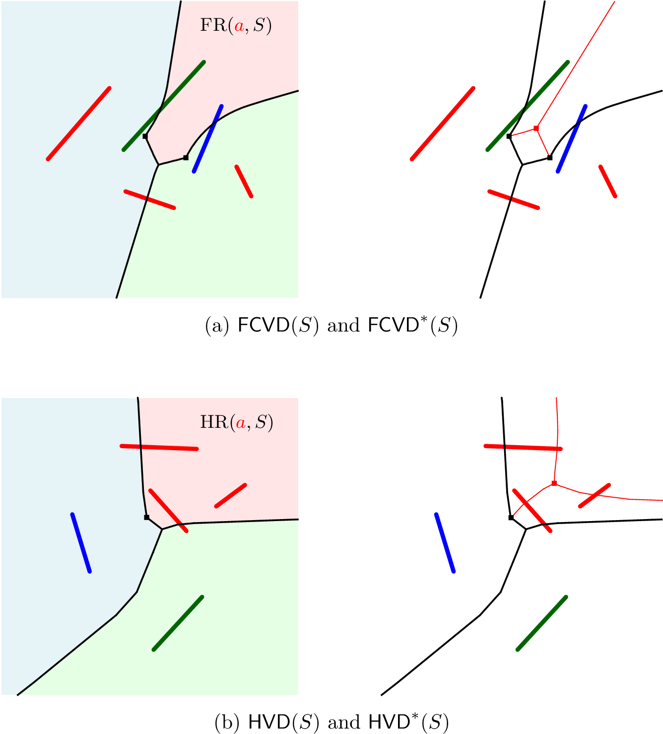
Our abstract definition of \(\mathsf{FCVD}(S)\) and \(\mathsf{HVD}(S)\) encompasses all concrete cases that have been studied before [23], [25], [26], [28], [40], including the farthest polygon Voronoi diagram [33], and any other case of generalized sites or metrics under the AVD model.
Refined order-\(k\) color diagrams.
We can analogously refine the order-\(k\) diagrams \(\mathsf{CVD}_k(S)\) and \(\overline{\mathsf{CVD}}_k(S)\), denoted by \(\mathsf{CVD}^*_k(S)\) and \(\overline{\mathsf{CVD}}^*_k(S)\), respectively, for each \(1\leqslant k\leqslant m\), where \(\mathsf{CVD}_m(S)\) and \(\overline{\mathsf{CVD}}_m(S)\) consist of a single region \(\mathrm{R}_m(K,S)=\overline{\mathrm{R}}_m(K,S)=\mathbb{R}^2\).
For each nonempty region \(R = \mathrm{R}_k(H, S)\) of \(\mathsf{CVD}_k(S)\), we overlay \(\mathsf{FCVD}^*(S_H)\) inside \(R\), where \(S_H = \bigcup_{a\in H} S_a\). The resulting refined diagram is denoted \(\mathsf{CVD}^*_k(S)\). Recall that \(\mathsf{FCVD}(S_H)=\mathsf{CVD}_{k-1}(S_H)\). Note that each face \(f\) of \(\mathsf{CVD}^*_k(S)\) is associated with a set \(H \subseteq K\) of \(k\) colors and a site \(p\in S_a\) for some color \(a\in H\) such that, at any point \(x\in f\), \(H\) is the common set of \(k\) nearest colors, color \(a\) is the \(k\)-th nearest color with respect to the minimal dominance \(\preccurlyeq_x\), and \(p \in S_a\) is the nearest site of color \(a\); that is, \(f \subseteq \mathrm{R}_k(H,S) \cap \mathsf{FCVD}(S_H) \cap \mathrm{VR}(p, S_a)\). See Figures 3 (d–g), where faces of \(\mathsf{CVD}^*_{k}(S)\) associated to the sites \(p\) and \(q\) are shaded purple and red, respectively.
For each nonempty region \(\overline{R} = \overline{\mathrm{R}}_k(H, S)\) of \(\overline{\mathsf{CVD}}_k(S)\), we overlay \(\mathsf{HVD}^*(S_H)\) inside \(\overline{R}\). The resulting refined diagram is denoted by \(\overline{\mathsf{CVD}}^*_k(S)\). Similarly as above, each face \(\bar{f}\) of \(\overline{\mathsf{CVD}}^*_k(S)\) is associated with a subset \(H \subseteq K\) of \(k\) colors and a site \(p\in S_a\) for some \(a\in H\) such that, at any point \(x\in \bar{f}\), \(H\) is the common set of \(k\) farthest colors, color \(a\) is the \(k\)-th farthest color with respect to the maximal dominance \(\mathrel{\overline{\succcurlyeq}}_x\), and \(p \in S_a\) is the farthest site among those in \(S_a\); that is, \(\bar{f} \subseteq \overline{\mathrm{R}}_k(H,S) \cap \mathsf{HVD}(S_H) \cap \mathrm{FVR}(p, S_a)\). See Figures 4 (d–g), where faces of \(\overline{\mathsf{CVD}}^*_{k}(S)\) associated to the sites \(p\) and \(q\) are also shaded purple and red.
Note \(\mathsf{CVD}^*_m(S) = \mathsf{FCVD}^*(S)\) and \(\overline{\mathsf{CVD}}^*_m(S) = \mathsf{HVD}^*(S)\), see Figures 3 (g) and 4 (g), whereas \(\mathsf{CVD}_{m-1}(S) = \mathsf{FCVD}(S)\) and \(\overline{\mathsf{CVD}}_{m-1}(S) = \mathsf{HVD}(S)\), see Figures 3 (c) and 4 (c).
Distinguishing chromatic features.
We can distinguish different features of the color diagrams by the number of their defining colors. Any edge or vertex of a color diagram is called \(c\)-chromatic, where \(c\in\{1,2,3\}\) is the number of distinct colors of the sites defining it. In \(\mathsf{CVD}_k(S)\) and \(\overline{\mathsf{CVD}}_k(S)\), Voronoi edges and their degree-\(2\) vertices are bichromatic (\(2\)-chromatic), while the Voronoi vertices are all trichromatic (\(3\)-chromatic). No monochromatic (\(1\)-chromatic) features exist in \(\mathsf{CVD}_k(S)\) or \(\overline{\mathsf{CVD}}_k(S)\).
As with ordinary order-\(k\) diagrams, the following properties are derived from definitions.
lemmaoverlayCVDkstar For each face \(R\subseteq \mathrm{R}_k(H,S)\) of \(\mathsf{CVD}_{k}(S)\), it holds: \(\mathsf{FCVD}(S_H) \cap R = \mathsf{CVD}_{k-1}(S) \cap R\). For each face \(\overline{R}\subseteq \overline{\mathrm{R}}_k(H,S)\) of \(\overline{\mathsf{CVD}}_k(S)\): \(\mathsf{HVD}(S_H) \cap \overline{R} = \overline{\mathsf{CVD}}_{k-1}(S) \cap \overline{R}\). Thus, superimposing \(\mathsf{CVD}_k(S)\) and \(\mathsf{CVD}_{k-1}(S)\) results in \(\mathsf{CVD}^*_{k}(S)\) with its monochromatic vertices and edges removed. Analogous statements hold for the maximal diagrams.
Proof. Since \(R\subseteq \mathrm{R}_k(H, S)\) and \(|H|=k\), it follows that \(\mathsf{CVD}_{k-1}(S) \cap R = \mathsf{CVD}_{k-1}(S_H) \cap R\). But \(\mathsf{CVD}_{k-1}(S_H)= \mathsf{FCVD}(S_H)\), thus, the first claim follows. Analogously, for \(\overline{R} \subseteq \overline{\mathrm{R}}_k(H, S)\), as \(\mathsf{HVD}(S_H) = \overline{\mathsf{CVD}}_{k-1}(S_H)\), while \(\overline{\mathsf{CVD}}_{k-1}(S)\cap \overline{R}=\overline{\mathsf{CVD}}_{k-1}(S_H)\cap \overline{R}\).
The superimposition property follows since \(\mathsf{CVD}^*_k(S) \cap R=\mathsf{FCVD}^*(S_H)\cap R\), and \(\mathsf{FCVD}(S_H)\cap R= \mathsf{CVD}_{k-1}(S_H)\) as already shown. ◻
A vertex or an edge of \(\mathsf{CVD}^*_k(S)\) or of \(\overline{\mathsf{CVD}}^*_k(S)\) is called new if it does not appear in \(\mathsf{CVD}^*_{k-1}(S)\) or in \(\overline{\mathsf{CVD}}^*_{k-1}(S)\), respectively; and old, otherwise. Note that vertices and edges of \(\mathsf{CVD}^*_1(S)\) and \(\overline{\mathsf{CVD}}^*_1(S)\) are all new, while those of \(\mathsf{CVD}^*_m(S)\) and \(\overline{\mathsf{CVD}}^*_m(S)\) are all old.
lemmaconsecutiveorders A \(c\)-chromatic vertex or edge appears in the diagrams \(\mathsf{CVD}^*_k(S)\) or \(\overline{\mathsf{CVD}}^*_k(S)\) for \(c\) consecutive orders, and in \(\mathsf{CVD}_k(S)\) or \(\overline{\mathsf{CVD}}_k(S)\) for \(c{-}1\) consecutive orders.
Proof. Consider a \(3\)-chromatic new vertex \(v\) of \(\mathsf{CVD}_k(S)\). By Lemma [lem:vertex95characterization], \(v\) is an old vertex in \(\mathsf{CVD}_{k+1}(S)\), and it does not appear in \(\mathsf{CVD}_{k+2}(S)\). In fact, it cannot appear in \(\mathsf{CVD}_{j}(S)\) for any \(j\notin \{k,k+1\}\) (see proof of Lemma [lem:vertex95characterization]). However, by Lemma [lem:overlay95CVDk95star], \(v\) appears in \(\mathsf{CVD}_{k+2}^*(S)\). Thus, the claim follows for \(c=3\).
Next, consider a \(2\)-chromatic edge \(e\) in \(\mathsf{CVD}_k(S)\) (and any \(2\)-chromatic vertex \(v\) that \(e\) may contain). By Lemma [lem:vertex95characterization], the edge \(e\) does not appear in \(\mathsf{CVD}_{k+1}(S)\), nor can it appear in any \(\mathsf{CVD}_{j}(S)\) for \(j\neq k\); however, it appears in \(\mathsf{CVD}^*_{k+1}(S)\), by Lemma [lem:overlay95CVDk95star]. Thus, the claim follows for \(c=2\).
Finally, consider a \(1\)-chromatic edge \(e\) (resp. vertex) defined by sites of color \(a\). By the definition of the refined diagrams, \(e\) appears in \(\mathsf{CVD}^*_k(S)\) if and only if \(a\) is the unique \(k\)-th nearest color of the points in \(e\). Thus, it appears in exactly \(1\) refined diagram. ◻
A full characterization of the \(c\)-chromatic features of \(\mathsf{CVD}^*_k(S)\) and \(\overline{\mathsf{CVD}}^*_k(S)\) can be established based on the ordering of sites in \(S\) with respect to \(\leqslant_x\) and the ordering of colors in \(K\) with respect to \(\preccurlyeq_x\).
lemmaedgetype For any \(x\in\mathbb{R}^2\), let \(p_1 \leqslant_x \cdots \leqslant_x p_n\) and \(a_1 \preccurlyeq_x \cdots \preccurlyeq_x a_m\) be the ordering of sites in \(S\) with respect to the relations \(\leqslant_x\) and the ordering of colors in \(K\) with respect to \(\preccurlyeq_x\), respectively.
Point \(x\) lies on a bichromatic edge of \(\mathsf{CVD}^*_k(S)\) if and only if \(a_{l-1} \prec_x a_l \sim_x a_{l+1} \prec_x a_{l+2}\) for \(l\in \{k-1, k\}\).
Point \(x\) lies on a monochromatic edge of \(\mathsf{CVD}^*_k(S)\) if and only if \(a_{k-1} \prec_x a_k \prec_x a_{k+1}\) and \(p_j =_x p_{j+1}\) for some \(j\) such that \(p_j, p_{j+1} \in S_{a_k}\) and \(p_i \notin S_{a_k}\) for all \(i<j\).
Proof. First, consider the bichromatic edges of \(\mathsf{CVD}^*_k(S)\). By Lemma [lem:overlay95CVDk95star], these are exactly the edges of \(\mathsf{CVD}_k(S)\) and of \(\mathsf{CVD}_{k-1}(S)\). It follows from Lemma [lem:basics95edge] and the general position assumption, that a point \(x\) on an edge \(e\) of \(\mathsf{CVD}_{k}(S)\) (resp. \(\mathsf{CVD}_{k-1}(S)\)) lies on the common boundary of two regions \(\mathrm{R}_k(H, S)\) and \(\mathrm{R}_k(H', S)\) (resp. \(\mathrm{R}_{k-1}(H, S)\) and \(\mathrm{R}_{k-1}(H', S)\)). By Lemma [lem:neighboring-regions], such an edge \(e\) is a portion of the bisector \(J({a},{a'})\) of the colors \(a \in H \setminus H'\) and \(a' \in H' \setminus H\). For a point \(x\) near \(e\) contained in \(\mathrm{R}_k(H, S)\) (resp. \(\mathrm{R}_{k-1}(H, S)\)), \(a\) and \(a'\) are the \(k\)-th and \((k{+}1)\)-th nearest colors (resp. \((k{-}1)\)-th and \(k\)-th) with respect to \(\preccurlyeq_x\). Thus, a point \(x\) lying on an edge of \(\mathsf{CVD}_{k}(S)\) (resp. \(\mathsf{CVD}_{k-1}(S)\)) implies \(a \sim_x a'\), where \(a = a_k\) and \(a' = a_{k+1}\) (resp. \(a = a_{k-1}\) and \(a' = a_{k}\)). Conversely, if these equivalence conditions hold at \(x\), any sufficiently small neighborhood of \(x\) intersects both adjacent regions, thus \(x\) must lie on their common boundary.
Next, consider a monochromatic edge \(e\) of \(\mathsf{CVD}^*_k(S)\), which is a monochromatic edge of \(\mathsf{FCVD}^*(S_H) \cap \mathrm{R}_k(H, S)\), \(H \subseteq K\). Furthermore, \(e\) lies strictly inside the region \(\mathrm{FR}(a, S_H)\) for some \(a \in H\). A point \(x\) is contained in \(\mathrm{R}_k(H, S) \cap \mathrm{FR}(a, S_H)\) if \(H\) is the set of \(k\) nearest colors from \(x\) and \(a\) is the unique farthest color in \(H\) with respect to \(\preccurlyeq_x\), implying that \(a = a_k\) and \(a_{k-1} \prec_x a_k \prec_x a_{k+1}\). A 1-chromatic edge \(e\) of \(\mathsf{FCVD}^*(S_H)\) inside \(\mathrm{FR}(a, S_H)\) is a portion of an edge of \(\mathsf{VD}(S_a)\). Under the general position assumption, \(x\) lying on an edge of \(\mathsf{VD}(S_a)\) means that \(x\) lies on the bisector \(J({p_j},{p_{j+1}})\) of the nearest sites \(p_j, p_{j+1} \in S_a\) with respect to \(\leqslant_x\). Therefore, \(p_j =_x p_{j+1}\) such that no \(p_i\) for \(i<j\) belongs to \(S_{a_k}\). The converse holds analogously: the strict color order ensures that the neighborhood around \(x\) is contained in \(\mathrm{R}_k(H, S)\), while the site equivalence implies it must lie on the bisector \(J({p_j},{p_{j+1}})\). ◻
lemmavertextype For any \(x\in\mathbb{R}^2\), let \(p_1 \leqslant_x \cdots \leqslant_x p_n\) and \(a_1 \preccurlyeq_x \cdots \preccurlyeq_x a_m\) be the ordering of sites in \(S\) with respect to the relations \(\leqslant_x\) and the ordering of colors in \(K\) with respect to \(\preccurlyeq_x\), respectively.
Point \(x\) is a \(3\)-chromatic vertex of \(\mathsf{CVD}^*_k(S)\) if and only if \(a_l \sim_x a_{l+1} \sim_x a_{l+2}\) for some \(l \in\{{k-2},k-1, k\}\).
Point \(x\) is a \(2\)-chromatic vertex of \(\mathsf{CVD}^*_k(S)\) if and only if \(a_l \sim_x a_{l+1}\) for some \(l \in \{k-1, k\}\), and \(p_j =_x p_{j+1} =_x p_{j+2}\) such that \(p_j, p_{j+1}, p_{j+2} \in S_{a_l} \cup S_{a_{l+1}}\) and \(p_i \notin S_{a_l} \cup S_{a_{l+1}}\) for all \(i<j\).
Point \(x\) is a \(1\)-chromatic vertex of \(\mathsf{CVD}^*_k(S)\) if and only if \(a_{k-1} \prec_x a_k \prec_x a_{k+1}\) and
[4] \(p_j =_x p_{j+1} =_x p_{j+2}\) such that \(p_j, p_{j+1}, p_{j+2}\in S_{a_k}\) and \(p_i \notin S_{a_k}\) for all \(i<j\).
Proof. First, consider the \(3\)-chromatic vertices of \(\mathsf{CVD}^*_k(S)\). By Lemma [lem:overlay95CVDk95star], these are exactly the vertices of \(\mathsf{CVD}_k(S)\) and \(\mathsf{CVD}_{k-1}(S)\). Recall from the proof of Lemma [lem:vertex95characterization] that \(x\) is a new vertex of \(\mathsf{CVD}_k(S)\) (resp. \(\mathsf{CVD}_{k-1}(S)\)) if \(a_k \sim_x a_{k+1} \sim_x a_{k+2}\) (resp. \(a_{k-1} \sim_x a_k \sim_x a_{k+1}\)), and \(x\) is an old vertex if \(a_{k-1} \sim_x a_k \sim_x a_{k+1}\) (resp. \(a_{k-2} \sim_x a_{k-1} \sim_x a_k\)). Thus, if \(x\) is a \(3\)-chromatic vertex then \(a_l \sim_x a_{l+1} \sim_x a_{l+2}\) for some \(l \in \{k-2, k-1, k\}\). The reverse implication can be proved analogously, as these equivalences imply the neighborhood of \(x\) intersects the three regions, defining a vertex.
Next, consider the \(2\)-chromatic vertices of \(\mathsf{CVD}^*_k(S)\), which must lie on the \(2\)-chromatic edges of \(\mathsf{CVD}^*_k(S)\). By Lemma [lem:edge95types], if a point \(x\) is on a \(2\)-chromatic edge of \(\mathsf{CVD}^*_k(S)\), then \(a_l \sim_x a_{l+1}\) for some \(l \in \{k-1, k\}\), and thus \(x \in J({a_l},{a_{l+1}})\). Since \(x\) is a vertex of \(J({a_l},{a_{l+1}})\), it is a vertex of \(\mathsf{VD}(S_{a_l} \cup S_{a_{l+1}})\) whose three nearest sites in \(S_{a_l} \cup S_{a_{l+1}}\), with respect to \(\leqslant_x\), include at least one site of color \(a_l\) and one of color \(a_{l+1}\). Under the general position assumption, a point \(x\) being a vertex of \(\mathsf{VD}(S_{a_l} \cup S_{a_{l+1}})\) implies it is equidistant to three sites \(p_j =_x p_{j+1} =_x p_{j+2}\) that are the nearest in \(S_{a_l} \cup S_{a_{l+1}}\) with respect to \(\leqslant_x\). Hence, \(p_j =_x p_{j+1} =_x p_{j+2}\) such that no \(p_i\) for \(i<j\) belongs to \(S_{a_l} \cup S_{a_{l+1}}\). Conversely, satisfying these equivalences implies that \(x\) lies on the common intersection of the three related bisecting curves.
Finally, consider the \(1\)-chromatic vertices of \(\mathsf{CVD}^*_k(S)\). As with the \(1\)-chromatic edges from Lemma [lem:edge95types], a \(1\)-chromatic vertex \(x\) has a unique \(k\)-th nearest color \(a_k\), so \(a_{k-1} \prec_x a_k \prec_x a_{k+1}\), and \(x\) is a vertex of \(\mathsf{VD}(S_{a_k})\). Under the general position assumption, being a vertex of \(\mathsf{VD}(S_{a_k})\) means \(x\) is equidistant from three sites \(p_j =_x p_{j+1} =_x p_{j+2}\) that are the nearest in \(S_{a_k}\) with respect to \(\leqslant_x\). Thus, no \(p_i\) for \(i<j\) belongs to \(S_{a_k}\). For the converse, the strict color ordering guarantees the neighborhood of \(x\) lies strictly inside the region where \(a_k\) is the \(k\)-th nearest color, while the site equivalence implies it is a vertex of the nearest-site Voronoi diagram. ◻
Using the maximal dominance relations \(\mathrel{\overline{\succcurlyeq}}_x\), \(\mathrel{\overline{\succ}}_x\), and \(\mathrel{\overline{\sim}}_x\), the vertices and edges of the maximal diagram \(\overline{\mathsf{CVD}}^*_k(S)\) can be characterized analogously.
A concrete example: the order-\(k\) polygon Voronoi diagram.
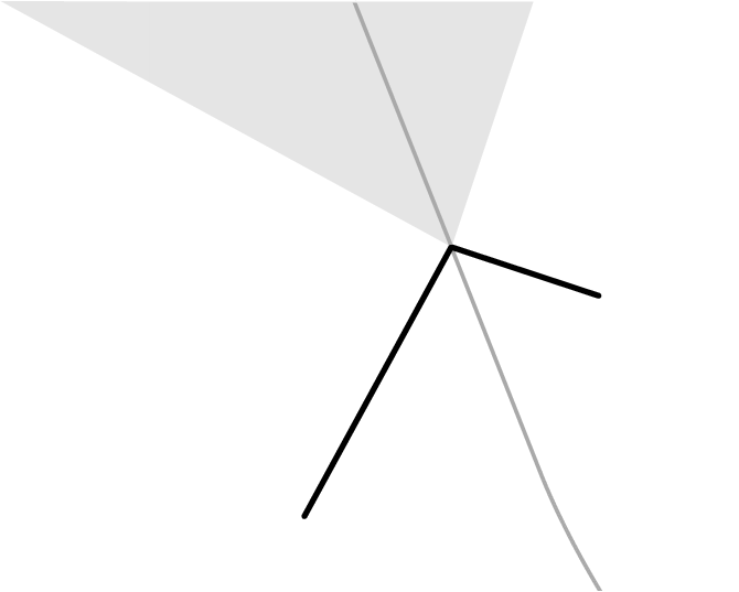
Let \(\mathcal{P}\) be a set of \(m\) disjoint simple polygons with a total of \(n\) vertices. Each polygon induces a distinct color in set \(K\). We can cast the order-\(k\) polygon Voronoi diagram as a concrete case of an order-\(k\) abstract color (minimal) Voronoi diagram, \(\mathsf{CVD}_k(S)\), by selecting the set \(S\) of sites so that the underlying bisector system is admissible. There are two ways to do so, each resulting in a slightly different (but equally valid) minimal refined diagram: (1) let \(S\) be a set of points and open line segments derived from the vertices and edges of the polygons in \(\mathcal{P}\); and (2) let \(S\) be a set of line segments derived from the polygonal edges in \(\mathcal{P}\). In the latter case, if two segments \(p\) and \(q\) have a common endpoint, then replace the two-dimensional portion of their bisector by the piece of their angular bisector contained in their equidistant area [41], see Figure 5. In both cases, the resulting families of bisecting curves are admissible as they satisfy the required axioms. Both definitions yield an identical \(\mathsf{CVD}_k(S)\), however, the corresponding refined diagrams \(\mathsf{CVD}^*_k(S)\) can have different monochromatic features.
The maximal diagram \(\overline{\mathsf{CVD}}_k(S)\) depends on which convention underlies the choice of \(S\). Under convention (1) \(\overline{\mathsf{CVD}}_k(S)\) reduces to a point maximal diagram \(\overline{\mathsf{CVD}}_k(S')\), where \(S'\subset S\) consists of the vertices in \(\mathcal{P}\); this is not the case under convention (2).
4 Combinatorial complexity↩︎
In this section, we establish the upper bound \(4k(n-k)-2n\), which is tight, for both minimal and maximal order-\(k\) abstract color Voronoi diagrams. Our proof is based on two techniques: (1) a random sampling technique, known as the Clarkson–Shor technique [34] with a colorful extension in [28]; and (2) a combinatorial analysis on the circular sequences of permutations induced by the unbounded edges of the order-\(k\) color Voronoi diagrams. Part (1) adapts the technique from [28] to abstract Voronoi diagrams and results in Lemma [lem:complexity]. Ppart (2) is detailed in Section 5 and its results are summarized in Lemma [lem:sumU].
We first introduce some notation. Consider the new vertices and the new unbounded edges of \(\mathsf{CVD}^*_k(S)\) and \(\overline{\mathsf{CVD}}^*_k(S)\), \(1\leqslant k\leqslant m\). Recall that a feature of an order-\(k\) diagram is called new if it does not appear in the diagram of order-\((k{-}1)\); and old, otherwise. Their numbers are denoted as follows.
Let \(\boldsymbol{v_{c,k}} = v_{c,k}(S)\) and \(\bar{v}_{c,k} = \bar{v}_{c,k}(S)\) denote the number of new \(c\)-chromatic vertices of \(\mathsf{CVD}^*_k(S)\) and of \(\overline{\mathsf{CVD}}^*_k(S)\), respectively.
Let \(\boldsymbol{u_{c,k}} = u_{c,k}(S)\) and \(\bar{u}_{c,k} = \bar{u}_{c,k}(S)\) denote the number of new \(c\)-chromatic unbounded edges of \(\mathsf{CVD}^*_k(S)\) and of \(\overline{\mathsf{CVD}}^*_k(S)\), respectively. Note that an edge that is unbounded in both directions is counted as two distinct unbounded edges. Also \(u_{c,m} = \bar{u}_{c,m} = 0\).
We now consider the first part of our proof whose results are summarized in Lemma [lem:complexity]. The Clarkson–Shor technique deals in general with a set system based on three ingredients: a set of \(n\) objects \(O\), a set of configurations \(\mathcal{F}(O)\), each defined by exactly \(d\) objects, and a conflict relation \(\chi \subseteq O \times \mathcal{F}(O)\), such that none of the \(d\) objects defining \(f\) are in conflict with \(f\). The set system defined by the triple \((O, \mathcal{F}(O), \chi)\) is called a CS-structure.
Given a CS-structure, suppose that the objects in \(O\) are colored by a color assignment \(\kappa \colon O \to K = \{1, \ldots, m\}\), where \(K\) is the set of \(m\leqslant n\) colors. In [28] a general framework was introduced, called the colorful Clarkson–Shor framework, which creates color-augmented CS-structures \((K,\mathcal{F}(O,\kappa), \chi_\kappa)\), such that the objects are colors, \(\mathcal{F}(O,\kappa) \subseteq \mathcal{F}(O)\) are colored configurations, and \(\chi_\kappa\) is a color-to-configuration conflict relation. The color-augmented CS-structure remains a CS-structure, therefore, the general random sampling technique of Clarkson and Shor [34] can still be applied.
We first observe the following from well-known properties of nearest and farthest abstract Voronoi diagrams [30], [39], under the general position assumption.
lemmavOuO For any subset \(S'\subseteq S\), the following hold: \[\sum_{1\leqslant c\leqslant 3} v_{c,1}(S') = 2|S'| - 2 - \sum_{1\leqslant c\leqslant 2} u_{c,1}(S') \quad\text{and}\quad \sum_{1\leqslant c\leqslant 3} \bar{v}_{c,1}(S') = \sum_{1\leqslant c\leqslant 2} \bar{u}_{c,1}(S') - 2.\]
Proof. The quantities \(\sum_{c} v_{c,1}(S')\) and \(\sum_c u_{c,1}(S')\) count the vertices and the unbounded edges, respectively, of the nearest Voronoi diagram \(\mathsf{CVD}^*_1(S')=\mathsf{VD}(S')\). The quantities \(\sum_{c} \bar{v}_{c,1}(S')\) and \(\sum_c \bar{u}_{c,1}(S')\) count the vertices and the unbounded edges, respectively, of the farthest Voronoi diagram \(\overline{\mathsf{CVD}}^*_1(S') = \mathsf{FVD}(S')\). Every region of \(\mathsf{VD}(S')\) is nonempty and simply connected [30] and every vertex is of degree three by the general position assumption. Euler’s formula thus implies the first equation. Every region of \(\mathsf{FVD}(S')\) is unbounded and \(\mathsf{FVD}(S')\) forms a tree [5], [39]. So, Euler’s formula together with the general position assumption implies the second equation. ◻
lemmacomplexity For each \(1 \leqslant k \leqslant m-1\), let \(U_k := \sum_{1\leqslant j \leqslant k} (u_{2,j} + (k-j+1) u_{1,j})\) and \(\overline{U}_k := \sum_{1\leqslant j \leqslant k} (\bar{u}_{2,j} + (k-j+1) \bar{u}_{1,j})\). The total number of vertices in \(\mathsf{CVD}_k(S)\) is exactly \[2k(2n-k)-2n - U_k - U_{k-1} - 2\sum_{j=1}^{k-1} v_{2,j} - \sum_{j=1}^{k} (2k-2j+1)v_{1,j}\] and the number of vertices in \(\overline{\mathsf{CVD}}_k(S)\) is exactly \[\overline{U}_k + \overline{U}_{k-1} - 2k^2 - 2\sum_{j=1}^{k-1}\bar{v}_{2,j}-\sum_{j=1}^{k}(2k-2j+1)\bar{v}_{1,j}.\]
Proof. Following [28], we first build two ordinary CS-structures for Voronoi vertices.
Let \(\mathcal{V}= \mathcal{V}(S)\) be the set of all Voronoi vertices created by any triplet of sites, i.e., vertices of \(\mathsf{VD}(\{p,q,r\})\) for any three distinct sites \(p,q,r\in S\), regardless of colors. Recall that there are at most two possible Voronoi vertices for each triplet of sites [30]. The set \(\mathcal{V}\) is the set of configurations. Consider two conflict relations \(\chi, \bar{\chi} \subseteq S \times \mathcal{V}\) defined as follows: for each \(p\in S\) and \(v\in \mathcal{V}\) whose defining sites are \(q_1,q_2, q_3\in S\), \[(p,v) \in \chi~\text{iff}~p <_v q_1 =_v q_2 =_v q_3 \quad\text{and}\quad (p,v) \in \bar{\chi}~\text{iff}~q_1 =_v q_2 =_v q_3 <_v p.\] The set systems \((S, \mathcal{V}, \chi)\) and \((S, \mathcal{V}, \bar{\chi})\) are CS-structures.
We then consider the color assignment \(\kappa \colon S \to K\) and derive two color-augmented CS-structures. Let \(\chi_\kappa, \bar{\chi}_\kappa \subseteq K \times \mathcal{V}\) be the corresponding color conflict relations with the following property: for each color \(a\in K\) and \(v\in\mathcal{V}\) defined by three sites \(q_1, q_2, q_3 \in S\), \[(a, v) \in \chi_\kappa~\text{iff}~a \prec_v \kappa(q_1) \sim_v \kappa(q_2) \sim_v \kappa(q_3) \;\text{and}\; (a, v) \in \bar{\chi}_\kappa~\text{iff}~a \mathrel{\overline{\succ}}_v \kappa(q_1) \mathrel{\overline{\sim}}_v \kappa(q_2) \mathrel{\overline{\sim}}_v \kappa(q_3).\]
By Lemma [lem:vertex95types], \(v\) is a new \(c\)-chromatic vertex of \(\mathsf{CVD}^*_{k}(S)\) if and only if \(v\) is a colored configuration induced by \((S, \mathcal{V}, \chi)\) such that \(v\) is in conflict with exactly \(k-1\) colors and \(c\) is equal to the number of distinct colors of the three sites defining \(v\). Analogously, \(v\) is a new \(c\)-chromatic vertex of \(\overline{\mathsf{CVD}}^*_{k}(S)\) if and only if \(v\) is a colored configuration induced by \((S, \mathcal{V}, \bar{\chi})\) such that \(v\) is in conflict with exactly \(k-1\) colors and \(c\) is equal to the number of distinct colors of three sites defining \(v\). Hence, the two color-augmented structures describe the new vertices of \(\mathsf{CVD}^*_k(S)\) and \(\overline{\mathsf{CVD}}^*_k(S)\).
Similarly, we can build two CS-structures encoding the new unbounded edges of \(\mathsf{CVD}^*_k(S)\) and of \(\overline{\mathsf{CVD}}^*_k(S)\). Recall the closed simple curve \(\Gamma\) enclosing \(\mathsf{CVD}^*_k(S)\) and \(\overline{\mathsf{CVD}}^*_k(S)\), defined in Section ¿sec:subsec:perm?. Let \(\mathcal{U} = \mathcal{U}(S)\) be the set of all intersection points between the bisectors in \(\mathcal{J}\) and \(\Gamma\). In this case, the set \(\mathcal{U}\) is the set of configurations. Each configuration \(u\in\mathcal{U}\) is defined by a unique pair of sites.
Consider two conflict relations \(\chi', \bar{\chi}' \subseteq S \times \mathcal{U}\): for each \(p\in S\) and \(u\in \mathcal{U}\) defined by \(q_1, q_2\in S\), \[(p,u) \in \chi'~\text{iff}~p <_u q_1 =_u q_2 \quad\text{and}\quad (p,u) \in \bar{\chi}'~\text{iff}~q_1 =_u q_2 <_u p.\] The set systems defined by the triplets \((S, \mathcal{U}, \chi')\) and \((S, \mathcal{U}, \bar{\chi}')\) form two CS-structures. The corresponding colored configurations induced by the color assignment \(\kappa\) for \(S\) describe the new \(c\)-chromatic unbounded edges in \(\mathsf{CVD}^*_k(S)\) and \(\overline{\mathsf{CVD}}^*_k(S)\), respectively. Specifically, let \(\chi'_\kappa, \bar{\chi}'_\kappa\) be the color-conflict relations corresponding to \(\chi'\) and \(\bar{\chi}'\), respectively. For each \(a\in K\) and \(u\in\mathcal{U}\) defined by two sites \(q_1, q_2 \in S\), \[(a, u) \in \chi'_\kappa~\text{iff}~a \prec_u \kappa(q_1) \sim_u \kappa(q_2) \quad\text{and}\quad (a, u) \in \bar{\chi}'_\kappa~\text{iff}~a \mathrel{\overline{\succ}}_u \kappa(q_1) \mathrel{\overline{\sim}}_u \kappa(q_2).\] By Lemma [lem:edge95types], we observe that a \(c\)-chromatic unbounded edge \(e\) in \(\mathsf{CVD}^*_{k}(S)\) is new if and only if the configuration \(u = e \cap \Gamma\) is in conflict with exactly \(k-1\) colors and \(c\) is equal to the number of distinct colors of the two sites defining \(u\). Analogously, \(u = e \cap \Gamma\) is a new \(c\)-chromatic unbounded edge of \(\overline{\mathsf{CVD}}^*_{k}(S)\) if and only if \(u\) is in conflict with exactly \(k-1\) colors and \(c\) is equal to the number of distinct colors of the two sites defining \(u\). Hence, the two color-augmented structures describe the new unbounded edges of the refined diagrams \(\mathsf{CVD}^*_k(S)\) and \(\overline{\mathsf{CVD}}^*_k(S)\).
From the lower bound lemma [28] (see also [34]), we have the following: For any integer \(1\leqslant r \leqslant m\) and a random subset \(R\subseteq K\) of \(r\) colors, \[\binom{m}{r} \mathop{\mathrm{\mathbf{E}}}[v_{c,1}(S_R)] = \sum_{j=0}^{m-c} v_{c,j+1}\binom{m-c-j}{r-c} \,\text{and}\, \binom{m}{r} \mathop{\mathrm{\mathbf{E}}}[\bar{v}_{c,1}(S_R)] = \sum_{j=0}^{m-c} \bar{v}_{c,j+1}\binom{m-c-j}{r-c}\] for each \(c \in \{1,2,3\}\), where \(S_R = \bigcup_{a\in R} S_a\), and \[\! \binom{m}{r} \mathop{\mathrm{\mathbf{E}}}[u_{c,1}(S_R)] = \sum_{j=0}^{m-c} u_{c,j+1}\binom{m-c-j}{r-c} \,\text{and}\, \binom{m}{r} \mathop{\mathrm{\mathbf{E}}}[\bar{u}_{c,1}(S_R)] = \sum_{j=0}^{m-c} \bar{u}_{c,j+1}\binom{m-c-j}{r-c}\] for each \(c\in\{1,2\}\). Hence, on one hand, we have \[\binom{m}{r}\left(\sum_{c=1}^3 \mathop{\mathrm{\mathbf{E}}}[v_{c,1}(S_R)] + \sum_{c=1}^2 \mathop{\mathrm{\mathbf{E}}}[u_{c,1}(S_R)]\right) = \sum_{c=1}^3 \sum_{j=0}^{m-c} (v_{c,j+1}+u_{c,j+1})\binom{m-c-j}{r-c}\] and \[\binom{m}{r}\left(\sum_{c=1}^3 \mathop{\mathrm{\mathbf{E}}}[\bar{v}_{c,1}(S_R)] - \sum_{c=1}^2 \mathop{\mathrm{\mathbf{E}}}[\bar{u}_{c,1}(S_R)]\right) = \sum_{c=1}^3 \sum_{j=0}^{m-c} (\bar{v}_{c,j+1}-\bar{u}_{c,j+1})\binom{m-c-j}{r-c},\] where we define \(u_{3,j} = \bar{u}_{3,j} = 0\) for all \(j\).
On the other hand, the upper bound lemma [28], together with Lemma [lem:v095u0], implies that \[\begin{align} \binom{m}{r}\left(\sum_{c=1}^3 \mathop{\mathrm{\mathbf{E}}}[v_{c,1}(S_R)] + \sum_{c=1}^2 \mathop{\mathrm{\mathbf{E}}}[u_{c,1}(S_R)]\right) &= \sum_{\substack{R'\subseteq K\\ |R'| = r}}\sum_{c=1}^3 (v_{c,1}(S_{R'}) + u_{c,1}(S_{R'})) \\ &= \sum_{R'} (2|S_{R'}| - 2) \\ & = 2\binom{m-1}{r-1}n - 2\binom{m}{r}, \end{align}\] for any \(2\leqslant r\leqslant m\). Similarly, we also have \[\binom{m}{r}\left(\sum_{c=1}^3 \mathop{\mathrm{\mathbf{E}}}[\bar{v}_{c,1}(S_R)] - \sum_{c=1}^2 \mathop{\mathrm{\mathbf{E}}}[\bar{u}_{c,1}(S_R)]\right) = - 2\binom{m}{r},\] for any \(2\leqslant r\leqslant m\).
These two sets of equations for \(2\leqslant r\leqslant m\) form two systems of linear equations, which are analogous to those in [28]. So, letting \[\begin{align} V_k := v_{3,k} + \sum_{j=1}^k (v_{2,j} + (k-j+1) v_{1,j}), \qquad & \overline{V}_k := \bar{v}_{3,k} + \sum_{j=1}^k (\bar{v}_{2,j} + (k-j+1) \bar{v}_{1,j}), \\ U_k := \sum_{j=1}^k (u_{2,j} + (k-j+1) u_{1,j}), \quad\text{and}\quad & \overline{U}_k := \sum_{j=1}^k (\bar{u}_{2,j} + (k-j+1) \bar{u}_{1,j}), \end{align}\] we obtain \[V_k + U_k = k(2n-k-1) \quad\text{and}\quad \overline{V}_k - \overline{U}_k = -k(k+1),\] for each \(1\leqslant j \leqslant m-1\). From Lemma [lem:consecutive95orders], for each \(1\leqslant k\leqslant m-1\), we know that the numbers of vertices of \(\mathsf{CVD}_k(S)\) and of \(\overline{\mathsf{CVD}}_k(S)\) are equal to \[v_{3,k} + v_{3,k-1} + v_{2,k} \quad\text{and}\quad \bar{v}_{3,k} + \bar{v}_{3,k-1} + \bar{v}_{2,k},\] respectively, where \(v_{3, 0} = \bar{v}_{3, 0} = 0\). Therefore, the claimed equations are derived analogously to [28]. ◻
Lemma [lem:complexity] reduces the problem of bounding the combinatorial complexity of \(\mathsf{CVD}_k(S)\) and \(\overline{\mathsf{CVD}}_k(S)\) to the problem of bounding two quantities \(U_k\) and \(\overline{U}_k\) regarding the number of new unbounded edges in the refined diagrams of orders \(1\) to \(k\). These equations were also derived in [28]. However, in [28] the two quantities \(U_k\) and \(\overline{U}_k\) were assumed equal, which holds in the case of point sites under convex distances. However, equality does not hold in general for other types of sites or metrics. In this paper we remove this assumption by establishing the following lemma whose proof is deferred to Section 5.
lemmasumU For each \(1\leqslant k\leqslant m-1\), \(U_k \geqslant k(k+1)\) and \(\overline{U}_k \leqslant k(2n-k-1)\). Both bounds are tight.
By combining Lemma [lem:complexity] and Lemma [lem:sumU] we obtain the following combinatorial result.
theoremthmcomplexity Let \(S\) be a set of \(n\) colored sites with \(m\leqslant n\) colors. Given an admissible system \(\mathcal{J}\) of bisecting curves for \(S\) and an integer \(k\) with \(1\leqslant k\leqslant m-1\), the total number of vertices in the order-\(k\) abstract color Voronoi diagram \(\mathsf{CVD}_k(S)\) or \(\overline{\mathsf{CVD}}_k(S)\) is at most \(4k(n-k)-2n\). Moreover, this bound is tight.
Proof. By Lemma [lem:complexity], the number of vertices in \(\mathsf{CVD}_k(S)\) is \[2k(2n-k) - 2n - U_k - U_{k-1} - 2\sum_{j=1}^{k-1} v_{2,j} - \sum_{j=1}^k(2k-2j+1)v_{1,j} \leqslant 4k(n-k) - 2n\] since \(U_k \geqslant k(k+1)\) as shown in Lemma [lem:sumU]. The number of vertices in \(\overline{\mathsf{CVD}}_k(S)\) is \[\overline{U}_k + \overline{U}_{k-1} - 2k^2 - 2\sum_{j=1}^{k-1} v_{2,j} - \sum_{j=1}^k(2k-2j+1)v_{1,j} \leqslant 4k(n-k) - 2n\] since \(\overline{U}_k \leqslant k(2n-k-1)\) as shown in Lemma [lem:sumU].
The tightness of the upper bound \(4k(n-k)-2n\) follows from the tightness of the bounds in Lemma [lem:sumU] and the fact that the number of \(c\)-chromatic vertices, \(c<3\), is zero if \(n=m\). ◻
The bound extends also (asymptotically) to the refined diagrams \(\mathsf{CVD}^*_k(S)\) and \(\overline{\mathsf{CVD}}^*_k(S)\) as \(O(k(n-k))\), following Lemma [lem:overlay95CVDk95star] and the fact that the monochromatic vertices are in total \(O(n)\).
Although the bound of Theorem [thm:complexity] is tight, \(\mathsf{FCVD}(S)\) and \(\mathsf{HVD}(S)\) may as well have linear complexity in special cases. In such cases the \(O(k(n-k))\) bound is not tight for large \(k\). We obtain a sharper asymptotic bound for \(m-k \in O(\sqrt{m})\) in the following theorem.
theoremlastorderscomplexity Given a set \(S\) of \(n\) colored sites with \(m\leqslant n\) colors and an admissible system \(\mathcal{J}\) of bisecting curves for \(S\), if \(\mathsf{FCVD}(S')\) (resp. \(\mathsf{HVD}(S')\)) has linear complexity for any \(S' \subseteq S\), then for each \(\lceil \frac{2m}{3} \rceil +1 \leqslant k\leqslant m-1\) the total combinatorial complexity of \(\mathsf{CVD}_{k}^*(S), \ldots, \mathsf{CVD}_{m}^*(S)\) (resp. \(\overline{\mathsf{CVD}}_{k}^*(S), \ldots, \overline{\mathsf{CVD}}_{m}^*(S)\)) is \(O((m-k)^2 n)\).
Proof. Recall the CS-structure \((S, \mathcal{V}, \chi)\) from the proof of Lemma [lem:complexity], where the set of configurations \(\mathcal{V}\) is the set of all possible Voronoi vertices, and the conflict relation \(\chi \subseteq S \times \mathcal{V}\) is defined such that a vertex \(v\in \mathcal{V}\) is in conflict with a site \(p \in S\) if and only if \(v\) is nearer to \(p\) than to the three sites defining \(v\). Recall also the color-augmented structure \((S, \mathcal{V}, \chi_\kappa)\), where \(\chi_\kappa \subseteq K \times \mathcal{V}\) is defined such that a \(c\)-chromatic vertex \(v\) is in conflict with a color \(a \in K\) if and only if \(v\) is nearer to \(a\), with respect to the minimal dominance \(\preccurlyeq_v\), than to the \(c\) colors of the sites defining \(v\).
We define a new color conflict relation \(\chi''_\kappa \subseteq K \times \mathcal{V}\) that is appropriate for large values of \(k\). For each color \(a \in K\) and vertex \(v \in \mathcal{V}\) defined by three sites \(q_1, q_2, q_3 \in S\): \[(a, v) \in \chi''_\kappa~\text{iff}~\kappa(q_1) \sim_v \kappa(q_2) \sim_v \kappa(q_3) \prec_v a.\] We call \(\{\kappa(q_1),\kappa(q_2),\kappa(q_3)\}\) the defining colors of the color configuration \(v\).
Let \(r = m-k+1\). The number of conflicts of a color configuration \(v\) with respect to \(\chi''_\kappa\) is the number of colors farther from \(v\) than its defining colors. A new \(c\)-chromatic vertex \(v\) of \(\mathsf{CVD}^*_k(S)\) has \(c\) defining colors, and \(k-1\) other colors closer than the defining colors; therefore, \(v\) has \(m-c-(k-1) = r-c\) colors farther from its defining colors. Let \(v''_{c,r-c+1}\) denote the number of \(c\)-chromatic vertices that are in conflict with exactly \(r-c\) colors with respect to \(\chi''_\kappa\). Note that \(v_{c,k} = v''_{c,r-c+1}\). From Lemma [lem:consecutive95orders], it follows that the total number of vertices in \(\mathsf{CVD}^*_k(S)\) is equal to \[\begin{align} {6} & v_{1,k} && + v_{2,k} && + v_{2,k-1} && + v_{3,k} && + v_{3,k-1} && + v_{3,k-2} \\ = \quad & v''_{1,r} && + v''_{2,r-1} && + v''_{2,r} && + v''_{3,r-2} && + v''_{3,r-1} && + v''_{3,r} \end{align}\] where \(v''_{3,-1} = v''_{3,0} = v''_{2,0} = 0\).
Assuming that \(\mathsf{FCVD}(S)\) has linear complexity, it follows that \(\sum_c v''_{c,1} = O(n)\). Note that for \(c=1\), the total number of monochromatic vertices is \(\sum_{r} v''_{1,r} = O(n)\). Theorem 4 in [28] applies to any color-augmented CS-structure, so it also applies to \((S,\mathcal{V},\chi''_\kappa)\). Let \(|\mathcal{F}_{c,j}(S, \chi''_\kappa)|\) denote the number of \(c\)-chromatic configurations that are in conflict with exactly \(j\) colors; observe that \(v''_{c,j+1} = |\mathcal{F}_{c,j}(S, \chi''_\kappa)|\). Applying the theorem with the function \(T_0(x)=x\) (since the complexity is linear for \(j=0\) and any \(S' \subseteq S\)), for each \(c \in \{2,3\}\) and \(1 \leqslant r \leqslant\lfloor m/c \rfloor\), the number of \(c\)-chromatic vertices with at most \(r-1\) conflicts is \[\sum_{j=0}^{r-1} v''_{c,j+1} = \sum_{j=0}^{r-1} |\mathcal{F}_{c,j}(S, \chi''_\kappa)| = O\left(\frac{r^c}{m} \cdot T_0\left(\frac{mn}{r}\right)\right) = O\left(\frac{r^c}{m} \cdot \frac{mn}{r}\right) = O(r^{c-1} n).\] Thus, the sum \(\sum_{j=0}^{r-1} v''_{c,j+1}\) for all \(c\in\{1,2,3\}\) is bounded by \(O(n + r n + r^2 n)\). Substituting \(r = m - k + 1\), the combinatorial complexity of \(\mathsf{CVD}_{k}^*(S), \ldots, \mathsf{CVD}_{m}^*(S)\) for \(\lceil \frac{2m}{3} \rceil +1 \leqslant k\leqslant m-1\) is \(O((m-k)^2 n)\).
Similarly, we define the color conflict relation \(\bar{\chi}''_\kappa \subseteq K \times \mathcal{V}\) for each color \(a \in K\) and vertex \(v \in \mathcal{V}\) defined by three sites \(q_1, q_2, q_3 \in S\): \[(a, v) \in \bar{\chi}''_\kappa~\text{iff}~\kappa(q_1) \mathrel{\overline{\sim}}_v \kappa(q_2) \mathrel{\overline{\sim}}_v \kappa(q_3) \mathrel{\overline{\succ}}_v a.\] The bound on \(\overline{\mathsf{CVD}}_{k}^*(S), \ldots, \overline{\mathsf{CVD}}_{m}^*(S)\) follows analogously. ◻
A concrete example is the order-\(k\) polygon Voronoi diagram of \(m\) disjoint simple polygons of total complexity \(n\), where the farthest polygon Voronoi diagram has complexity \(O(n)\) [33].
Corollary 1. Given a collection of \(m\) disjoint simple polygons of \(n\) total vertices and an integer \(k\) with \(1\leqslant k\leqslant m-1\), the order-\(k\) polygon Voronoi diagram has combinatorial complexity \(O(\min\{k(n-k),(m-k)^2n\})\).
5 Tight bounds on \(U_k\) and \(\overline{U}_k\) – Proving Lemma [lem:sumU]↩︎
Recall the circular sequence \(\Pi(S) = (\pi_0, \ldots, \pi_{N-1}, \pi_N=\pi_0)\) of permutations \(\pi_i\) of sites \(S\), discussed in Section ¿sec:subsec:perm?. In our setting, each site \(p\in S\) is assigned a color \(\kappa(p) \in K\). For each color \(a\in K\) and \(0\leqslant i\leqslant N-1\), let \(\lambda_i(a) \in S_a\) be the first site of color \(a\) in permutation \(\pi_i\), called the leader of color \(a\) in \(\pi_i\). By a slight abuse of notation, we also use \(\lambda_i\) to denote the subsequence of \(\pi_i\) that consists of the leaders of all colors. It is not hard to see that the induced circular sequence \(\Lambda(\Pi(S)) = (\lambda_0, \ldots, \lambda_N = \lambda_0)\) of color-leader sequences satisfies exactly one of the following, if \(\lambda_{i+1} \neq \lambda_i\):
(L1)
there is a replacement of the leader of a color \(a\in K\), that is, \(\lambda_{i+1}(a) \neq \lambda_i(a)\), or
(L2)
there is a switch of two consecutive leaders from \(\lambda_i\) to \(\lambda_{i+1}\),
A change of the first kind (L1) is called a monochromatic switch as it corresponds to a switch in \(\Pi(S)\) between two sites of the same color; a change of the second kind (L2) is called a bichromatic switch. We say that a monochromatic switch happens at position \(j\), if the leader \(\lambda_i(a)\) of a color \(a\in K\) is at position \(j\) in \(\lambda_i\), and that a bichromatic switch happens at positions \(j\), if two leaders \(\lambda_i(a)\) and \(\lambda_i(b)\) (to be switched) lie at positions \(j\) and \(j+1\) in \(\lambda_i\). We then observe the following correspondence between unbounded edges and switches.
lemmaUG Let \(\overline{\Pi}(S) := (\bar{\pi}_0, \ldots, \bar{\pi}_N = \bar{\pi}_0)\), where \(\bar{\pi}_i\) denotes the reverse of permutation \(\pi_i\). For each \(1\leqslant k\leqslant m\), the following hold for the \(c\)-chromatic unbounded edges, \(c\in\{1,2\}\):
\(u_{c,k}\) is equal to the number of \(c\)-chromatic switches at position \(k\) in \(\Lambda(\Pi(S))\).
\(\bar{u}_{c,k}\) is equal to the number of \(c\)-chromatic switches at position \(k\) in \(\Lambda(\overline{\Pi}(S))\).
Proof. The proof is done by establishing one-to-one correspondences between:
The set of new monochromatic unbounded edges of \(\mathsf{CVD}^*_k(S)\) and the set of monochromatic switches at position \(k\) in \(\Lambda(\Pi(S))\).
The set of new bichromatic unbounded edges of \(\mathsf{CVD}^*_k(S)\) and the set of bichromatic switches at position \(k\) in \(\Lambda(\Pi(S))\).
The set of new monochromatic unbounded edges of \(\overline{\mathsf{CVD}}^*_k(S)\) and the set of monochromatic switches at position \(k\) in \(\Lambda(\overline{\Pi}(S))\).
The set of new bichromatic unbounded edges of \(\overline{\mathsf{CVD}}^*_k(S)\) and the set of bichromatic switches at position \(k\) in \(\Lambda(\overline{\Pi}(S))\).
Let \(x \in \Gamma\), and let \(a_1 \preccurlyeq_x \cdots \preccurlyeq_x a_m\) and \(p_1 \leqslant_x \cdots \leqslant_x p_n\) be the ordering of colors in \(K\) with respect to \(\preccurlyeq_x\) and the ordering of sites in \(S\) with respect to \(\leqslant_x\), respectively.
Suppose that it holds that \(a_{k-1} \prec_x a_k \prec_x a_{k+1}\) and \(p_{j-1} <_x p_j =_x p_{j+1} <_x p_{j+2}\) for some \(j\) such that \(p_j, p_{j+1} \in S_{a_k}\), and \(p_i \notin S_{a_k}\) for all \(i<j\). Then \(p_j, p_{j+1}\) are the nearest sites among those in \(S_{a_k}\) at \(x\). Thus, \(x = e\cap \Gamma\) for a new monochromatic unbounded edge \(e\) of \(\mathsf{CVD}^*_k(S)\) (see also Lemma [lem:edge95types]). At the same time, \(x \in \Gamma\) corresponds to the switch \(\sigma\) of \(p_j\) and \(p_{j+1}\) between two consecutive permutations \(\pi_i,\pi_{i+1} \in \Pi(S)\). As both \(p_j\) and \(p_{j+1}\) belong to the same color \(S_{a_k}\) and \(a_k\) is the \(k\)-th nearest color locally near \(x\), the switch \(\sigma\) is monochromatic happening at position \(k\) by which the leader of color \(a_k\) is replaced between \(\lambda_i\) and \(\lambda_{i+1}\). Conversely, any monochromatic switch of \(p_j\) and \(p_{j+1}\) of color \(a_k\) happening at position \(k\) corresponds to a point \(x\in \Gamma\) that satisfies the above condition. This establishes the first one-to-one correspondence between the set of new monochromatic unbounded edges of \(\mathsf{CVD}^*_k(S)\) and the set of monochromatic switches at position \(k\) in \(\Lambda(\Pi(S))\), implying that the number of monochromatic switches at position \(k\) in \(\Lambda(\Pi(S))\) is exactly \(u_{1,k}\).
Next, if it holds that \(a_{k-1} \prec_x a_k \sim_x a_{k+1} \prec_x a_{k+2},\) then \(x \in \mathop{\mathrm{cl}}\mathrm{R}_k(H, S) \cap \mathop{\mathrm{cl}}\mathrm{R}_k(H',S)\) for \(H = \{a_1, \ldots, a_k\}\) and \(H' = H \cup \{a_{k+1}\} \setminus \{a_{k}\}\). Thus \(x = e \cap \Gamma\) for a new bichromatic unbounded edge \(e\) of \(\mathsf{CVD}^*_k(S)\) (see Lemma [lem:edge95types]). At the same time, \(x\) corresponds to the switch of the leaders of two colors \(a_k\) and \(a_{k+1}\) between two consecutive sequences \(\lambda_i\) and \(\lambda_{i+1}\) of color leaders, so a bichromatic switch at position \(k\). Conversely, for any bichromatic switch at position \(k\) corresponding to a point \(x\in\Gamma\), we have the same condition as above at \(x\), so \(x\) lies on a new bichromatic unbounded edge of \(\mathsf{CVD}^*_k(S)\). This implies that the number of bichromatic switches at position \(k\) in \(\Lambda(\Pi(S))\) is equal to \(u_{2,k}\).
The other two cases for the maximal diagrams \(\overline{\mathsf{CVD}}^*_k(S)\) can be shown analogously using the sequence \(\overline{\Pi}(S)\) of reversed permutations. Let \(\bar{\lambda}_i\) be the sequence of color leaders induced from the reversed permutation \(\bar{\pi}_i\) such that \(\Lambda(\overline{\Pi}(S)) = (\bar{\lambda}_0, \ldots, \bar{\lambda}_{N-1}, \bar{\lambda}_N=\bar{\lambda}_0)\). Notice that the \(k\)-th farthest color with respect to the maximal dominance \(\mathrel{\overline{\succcurlyeq}}_x\) is at position \(k\) in the corresponding color-leader sequence \(\bar{\lambda}_i\). Hence, the characterization of new edges of \(\overline{\mathsf{CVD}}^*_k(S)\), analogous to Lemma [lem:edge95types], implies the last two correspondences between new unbounded edges of \(\overline{\mathsf{CVD}}^*_k(S)\) and switches at position \(k\) in \(\Lambda(\overline{\Pi}(S))\). Consequently, the number of monochromatic switches at position \(k\) in \(\Lambda(\overline{\Pi}(S))\) is equal to \(\bar{u}_{1,k}\), while the number of bichromatic switches at position \(k\) in \(\Lambda(\overline{\Pi}(S))\) is equal to \(\bar{u}_{2,k}\). ◻
Thus, to obtain the bounds of Lemma [lem:sumU], it is enough to count monochromatic and bichromatic switches in the circular sequences \(\Lambda(\Pi(S))\) and \(\Lambda(\overline{\Pi}(S))\) of color-leaders. We do the counting in a purely combinatorial setting in the next subsection deriving the bounds of Theorem [thm:Gk]. As a corollary to Theorem [thm:Gk] we get: \(U_k \geqslant k(k+1)\) and \(\overline{U}_k \leqslant k(2n-k-1)\). These bounds are tight for the unbounded edges of the diagrams by the fact that any circular sequence \(\Pi\) of permutations satisfying conditions (P1) and (P2) can be realized by an admissible system of bisecting curves [5]. This completes the proof of Lemma [lem:sumU].
5.1 Switches in a sequence of permutations of colored elements↩︎
In the following, we consider a purely combinatorial setting for circular sequences as follows. Let \(\Pi = (\pi_0, \ldots, \pi_N = \pi_0)\) be a given circular sequence of permutations \(\pi_i\) of \(n\) elements \(\{1, \ldots, n\}\) that satisfies conditions (P1) and (P2), and assume that each element in \(\{1, \ldots, n\}\) is assigned a color from \(K =\{1, \ldots, m\}\). As above, we have the induced sequence \(\Lambda = \Lambda(\Pi) = (\lambda_0, \ldots, \lambda_{N-1},\lambda_N=\lambda_0)\) of sequences \(\lambda_i\) of \(m\) leaders of colors, which satisfy conditions (L1) and (L2). For each \(1\leqslant k\leqslant m\), define \(\boldsymbol{g_{1,k}} = g_{1,k}(\Pi)\) to be the number of monochromatic switches at position \(k\) in \(\Lambda\) and \(\boldsymbol{g_{2,k}} = g_{2,k}(\Pi)\) to be the number of bichromatic switches at position \(k\) in \(\Lambda\). We are interested in the following quantity: \[G_k = G_k(\Pi) := \sum_{j=1}^k ( g_{2,j} + (k-j+1) g_{1,j}).\]
theoremGk For \(1\leqslant k\leqslant m-1\), \(k(k+1)\leqslant G_k\leqslant k(2n-k-1)\). Both bounds are tight.
The bounds are shown to be tight by constructions, see Lemma [lem:Gk95tight].
5.1.1 Deriving the lower bound↩︎
We charge each monochromatic or bichromatic switch to a unique color \(a\in K\) as follows:
Each monochromatic switch, replacing the leader of color \(a\in K\), is charged to the corresponding color \(a\). Let \(\boldsymbol{\mu_a(j)}\) be the number of monochromatic switches at position \(j\) in \(\Lambda\) charged to \(a\).
Each bichromatic switch involving two colors \(a,a' \in K\) with \(a< a'\) is charged to color \(a\) with the smaller index. Let \(\boldsymbol{\beta_a(j)}\) be the number of bichromatic switches at position \(j\) in \(\Lambda\) charged to \(a\).
It is obvious that \(g_{1,j} = \sum_{a\in K} \mu_a(j)\) and \(g_{2,j} = \sum_{a\in K} \beta_a(j)\).
Let \(\rho_i(a)\) for \(a\in K\) be the position, or the rank, of \(\lambda_i(a)\) in permutation \(\lambda_i\), and let \(\rho^*(a) := \max_{i} \rho_i(a)\) be the maximum rank of \(a\) over the whole sequence \(\Lambda\). Note that for any color \(a\in K\) having a single element, we have \(\mu_a(j) = 0\) for every \(j\), since there is no change of its leader \(\lambda_i(a)\). We observe the following for colors having at least two elements.
lemmamcineqtwosites Let \(a \in K\) be any color having at least two elements. For \(1\leqslant k\leqslant m-1\), \[\sum_{j=1}^k (k-j+1) \mu_a(j) \geqslant\max \{2(k + 1 - \rho^*(a)), 0\}.\]
Proof. If \(k < \rho^*(a)\), then \(\max \{k + 1 - \rho^*(a), 0\} = 0\) and the inequality holds trivially, so assume \(k \geqslant\rho^*(a)\).
We first observe that there are at least two changes of \(\lambda_i(a)\) over \(0\leqslant i\leqslant N-1\). This is obvious from the fact that \(\lambda_i(a)\) is the first element of the subsequence of \(\pi_i\) that contains those elements in \(\{1, \ldots, n\}\) whose color is \(a\) and the property (P2) that every pair of elements switches exactly twice.
Consider any two such changes happened at \(0\leqslant i_1 < i_2 < N\), and let \(j_1:=\rho_{i_1}(a)\) and \(j_2:=\rho_{i_2}(a)\) be two positions of the leader of \(a\) in \(\lambda_{i_1}\) and \(\lambda_{i_2}\), respectively. By definition, we have \(j_1, j_2 \leqslant\rho^*(a) \leqslant k\). Thus, we obtain \[\sum_{j=1}^k (k-j+1) \mu_a(j) \geqslant(k-j_1+1) + (k-j_2+1) \geqslant 2 (k - \rho^*(a) +1)\] by the existence of two changes of \(\lambda_i(a)\). ◻
Next, we consider the quantity \(\beta_a(j)\) about bichromatic switches. Note that \(\beta_a(m) = 0\) for any \(a\in K\) and \(\beta_m(k) = 0\) for any \(k\) by definition. From here onward, we assume without loss of generality that \(\pi_0 = (1, 2, \ldots, n)\) and the colors in \(K =\{1, \ldots, m\}\) appear in the order in the initial permutation \(\lambda_0\) of leaders, that is, \(\lambda_0 = (\lambda_0(1), \lambda_0(2), \ldots, \lambda_0(m))\), so \(\rho_0(a) = a\) for \(a\in K = \{1, \ldots, m\}\).
lemmabiineq For \(1 \leqslant k \leqslant m-1\) and \(a \in K\), it holds that \(\sum_{j=1}^k \beta_a(j) \geqslant\max\{2 ( \hat{k}_a + 1 - a ), 0\}\), where \(\hat{k}_a = \min\{ k, \rho^*(a)-1 \}\).
Proof. Recall our assumption that the leader of color \(a\) is placed at position \(a\) in \(\lambda_0\), that is, \(\rho_0(a) = a\). If \(\hat{k}_a < a - 1\), then the inequality holds trivially, so assume that \(\hat{k}_a \geqslant a\).
Let \(z\) be an index such that \(\rho_z(a) = \hat{k}_a + 1\), and let \[A := \{ a'\in K \mid a' > a~\text{and}~\rho_z(a') < \rho_z(a) = \hat{k}_a+1 \}.\] be the set of colors \(a' > a\) preceding \(a\) in \(\lambda_z\). Since the order between colors \(a\) and each \(a' \in A\) is reversed between \(\lambda_0\) and \(\lambda_z\), there must be at least \(|A|\) many bichromatic switches while we move from \(\lambda_0\) to \(\lambda_z\), counted in \(\sum_{j=1}^{\hat{k}_a} \beta_a(j)\). On the other hand, while we move from \(\lambda_z\) to \(\lambda_N = \lambda_0\), this order between \(a\) and each \(a'\in A\) should be reversed again. This implies that \[\sum_{j=1}^k \beta_a(j) \geqslant\sum_{j=1}^{\hat{k}_a} \beta_a(j) \geqslant 2|A|.\]
To bound \(|A|\), let \(B := \{ a'\in K \mid a' < a~\text{and}~\rho_z(a') < \rho_z(a)\}\). Obviously, \(|B| \leqslant a-1\) and \(A\cap B =\emptyset\). Since \(A\cup B\) consists of all colors \(a'\) such that \(\rho_z(a') < \rho_z(a) = \hat{k}_a + 1\), we have \(|A\cup B| = \hat{k}_a\) and hence \[|A| = |A\cup B| - |B| \geqslant\hat{k}_a - (a - 1) = \hat{k}_a + 1 - a,\] implying the inequality. ◻
For colors \(a\in K\) that have only a single element, we show a better lower bound on \(\beta_a\) in the next lemma. By combining we derive the inequality in Lemma [lem:sub-goal].
lemmabiineqonesite Let \(a \in K\) be a color having only one element. For \(1\leqslant k\leqslant m-1\), it holds that \(\sum_{j=1}^k \beta_a(j) \geqslant\max\{2 ( k + 1 - a ), 0\}\).
Proof. Let \(t \in\{1, \ldots, n\}\) be the only element of color \(a\), so \(t\) is always the leader of \(a\): \(\lambda_i(a) = t\) for all \(i\). Since every pair of elements switch exactly twice in the sequence \(\Pi\) (condition (P2)), \(t\) is involved in at least two bichromatic switches with each of the other colors. Among them, those switches with \(a' > a\) are counted in \(\sum_j \beta_a(j)\), so we have \[\sum_j \beta_a(j) = \sum_{j=1}^{\rho^*(a)} \beta_a(j) \geqslant 2(m-a).\]
We have two cases: whether \(k \geqslant\rho^*(a)\) or \(k < \rho^*(a)\). If \(k \geqslant\rho^*(a)\), then we have \[\sum_{j=1}^{k} \beta_a(j) \geqslant\sum_{j=1}^{\rho^*(a)} \beta_a(j) \geqslant 2 (m - a) \geqslant\max\{2 ( k + 1 - a ), 0\}\] since \(k \leqslant m-1\). Otherwise, if \(k < \rho^*(a)\), then Lemma [lem:bi95ineq] is strong enough to conclude the lemma: \[\sum_{j=1}^k \beta_a(j) \geqslant\max\{2 ( \hat{k}_a + 1 - a ), 0\} \geqslant\max\{2 ( k + 1 - a ), 0\}\] since \(\hat{k}_a = \min\{k, \rho^*(a) - 1\} = k\). ◻
lemmasubgoal For \(1 \leqslant k \leqslant m-1\) and \(a \in K\), it holds that \[\sum_{j=1}^{k} \beta_a(j) + \sum_{j=1}^{k} (k-j+1) \mu_a(j) \geqslant\max\{2(k+1-a)), 0\}.\]
Proof. If there is only one element in \(\{1, \ldots, n\}\) whose color is \(a\), then \(\mu_a(j) = 0\) for all \(j\), so Lemma [lem:bi95ineq95195site] implies the lemma. So, in the following, we assume that there are at least two elements whose color is \(a\).
Adding the inequalities of Lemmas [lem:mc95ineq95295sites] and [lem:bi95ineq] yields \[\sum_{j=1}^{k} \beta_a(j) + \sum_{j=1}^{k} (k-j+1)\mu_a(j) \geqslant\max\{2 (\hat{k}_a + 1 - a), 0\} + \max\{2 ( k + 1 - \rho^*(a) ), 0\}.\]
We simplify the right-hand side by a case analysis on \(\hat{k}= \min\{k, \rho^*(a)-1\}\). If \(\rho^*(a) \leqslant k\), then \(\hat{k}_a = \rho^*(a)-1\) and \(\hat{k}_a + 1 - a = \rho^*(a) - a\). Note also the trivial fact that \(\rho^*(a) - a = \rho^*(a) - \rho_0(a) \geqslant 0\). So, the right-hand side is simplified to \[2(\rho^*(a)-a) + \max\{2(k-\rho^*(a)+1),0\} = \max\{2(k + 1 - a), 0\}.\] Otherwise, if \(\rho^*(a) > k\), then \(\hat{k}_a = k\) and \(\max\{2 ( k + 1 - \rho^*(a)), 0\} = 0\). So, we have \[\max\{2 (\hat{k}_a + 1 - a), 0\} + \max\{2 ( k + 1 - \rho^*(a) ), 0\} = \max\{2 ( k + 1 - a ), 0\},\] as claimed. ◻
Summing the inequality of Lemma [lem:sub-goal] over all colors \(a\in K\), we obtain the claimed lower bound of Theorem [thm:Gk], as \(\sum_{a\in K} \mu_a(j) = g_{1,j}\) and \(\sum_{a\in K} \beta_a(j) = g_{2,j}\). Specifically, we have \[G_k = \sum_{a\in K}\sum_{j=1}^k (\beta_a(j) + (k-j+1)\mu_a(j)) \geqslant\sum_{a=1}^m \max\{2(k+1-a), 0\} = 2 \sum_{a=1}^k a = k(k+1).\]
5.1.2 Deriving the upper bound↩︎
Recall our assumption that \(\pi_0 = (1,2, \ldots, n)\) and \(\lambda_0 = (\lambda_0(1), \ldots, \lambda_0(m))\) as above. We start with the following observation.
lemmamslast For \(a\in K\), the largest element \(t\) of color \(a\) can be the leader of \(a\) at most once in \(\pi_i\) over all \(0\leqslant i\leqslant N\). Thus, \(t\) is involved in exactly zero or two monochromatic switches.
Proof. If \(t\) is the only element of color \(a\), then the lemma is trivially true, since \(\lambda_i(a) = t\) for all \(i\) and thus there is no monochromatic switches involving \(t\). So, assume there is at least one more element \(t' < t\) of the same color \(a\). Let \(T_a\) be the set of elements \(t'\) whose colors are commonly \(a\). Consider the subsequence \(\tau_i\) of \(\pi_i\) that contains the elements in \(T_a\). Observe that \(t\) is at the first position in \(\tau_i\) if and only if \(t = \lambda_i(a)\).
Now, suppose that \(t = \lambda_i(a)\) for some \(i\). Since \(t\) is at the last position in the initial permutation \(\tau_0\), in order for \(t\) to step forward to the first position, every other member in \(T_a\) has to be switched with \(t\), and then they have to be switched with \(t\) again by condition (P2) which requires that every pair of elements is switched exactly twice in \(\Pi\). If the second switch between \(t\) and any \(t' \in T\) happens in \(\tau_z\) at some \(0\leqslant z\leqslant N-1\), then \(t'\) precedes \(t\) in \(\tau_i\) for any \(z< i \leqslant N-1\). This proves the lemma. ◻
To prove the upper bound of \(G_k\), we introduce another charging scheme, in which every switch of our interest is charged to a unique element \(t\in\{1, \ldots, n\}\) as follows.
Every monochromatic switch in \(\Lambda\) induced by a switch of elements \(t\) and \(t'\) with \(1\leqslant t' < t \leqslant n\) in \(\Pi\) is charged to element \(t\) with the larger index. Let \(\boldsymbol{\hat{\mu}_t(j)}\) be the number of monochromatic switches at position \(j\) in \(\Lambda\) charged to element \(t\).
Every bichromatic switch in \(\Lambda\) induced by a switch of elements \(t\) and \(t'\) with \(1\leqslant t' < t \leqslant n\) in \(\Pi\) is charged to element \(t\) with the larger index. Let \(\boldsymbol{\hat{\beta}_t(j)}\) be the number of bichromatic switches at position \(j\) in \(\lambda\) charged to element \(t\).
In short, each monochromatic and bichromatic switch is charged to the involved element \(t\) of the larger index. Obviously, we have \(g_{1,j} = \sum_{1\leqslant t\leqslant n} \hat{\mu}_t(j)\) and \(g_{2,j} = \sum_{1\leqslant t\leqslant n} \hat{\beta}_t(j)\).
The following is an immediate implication of Lemma [lem:ms95last].
lemmabarmc For \(1\leqslant t\leqslant n\), \(\sum_{j=1}^{m} \hat{\mu}_t(j) \leqslant 2\); if \(t = \lambda_0(a)\) for \(a\in K\), then \(\sum_{j=1}^{m} \hat{\mu}_t(j) = 0\).
Proof. If \(t = \lambda_0(a)\) is the initial leader of color \(a\), then there is no other element \(t' < t\) of the same color \(a\). Hence, there is no monochromatic switch contributed to \(\hat{\mu}_t(j)\) for all \(j\). So, we assume that \(t\) is in color \(a\) and there is at least one more element \(t' < t\) of the same color \(a\). Here, we redefine \(T_a\) to be the set of elements \(t' \leqslant t\) whose colors are commonly \(a\), and consider the subsequence \(\tau_i\) of \(\pi_i\) that contains the elements in \(T_a\), as in the proof of Lemma [lem:ms95last]. Observe that any monochromatic switch in \(\Lambda\) involving \(t\) corresponds to a switch between the first and second positions that involves \(t\) in the \(\tau_i\)’s, while the converse is not necessarily true. Hence, we have \(\sum_{j=1}^{m} \hat{\mu}_t(j) \leqslant 2\) by Lemma [lem:ms95last]. ◻
lemmabarsubgoal For \(1 \leqslant k \leqslant m-1\) and \(1\leqslant t\leqslant n\), it holds that \[\sum_{j=1}^{k} (\hat{\beta}_t(j) + (k-j+1) \hat{\mu}_t(j)) \leqslant \begin{cases} 2 \min\{a-1, k\} & \text{if}~t=\lambda_0(a)~\text{for}~a\in K\\ 2k & \text{otherwise} \end{cases}\]
Proof. First, assume that \(t=\lambda_0(a)\) for some color \(a\in K\). Note, by Lemma [lem:bar95mc], that \(\sum_j \hat{\mu}_t(j)=0\), so we are interested in an upper bound of \(\sum_{j=1}^k \hat{\beta}_t(j)\). Let \(T = \{1, \ldots, t\}\) be the set of elements preceding \(t\) in \(\pi_0\), including \(t\). We consider another circular sequence \(\Pi' = (\pi'_0, \ldots, \pi'_{N-1})\) of permutations \(\pi'_i\) of \(T\) such that \(\pi'_i\) is the subsequence of \(\pi_i\) that contains the elements in \(T\). We also let \(\Lambda' = \Lambda(\Pi') = (\lambda'_0, \ldots, \lambda'_{N-1})\) be the sequence of color leaders induced from \(\Pi'\). Note that each bichromatic switch in \(\Lambda\) counted in the sum \(\sum_{j} \hat{\beta}_t(j)\) corresponds to a bichromatic switch in \(\Lambda'\) involving \(t\), since \(t\) is the largest element in \(T\) and we charge each switch in \(\Lambda\) to the larger element of the two involved elements. Hence, it suffices for our purpose to have an upper bound on the number of bichromatic switches involving \(t\) in \(\Lambda'\).
Let \(T_b \subseteq T\) for \(b \in K\) be the set of elements in \(T\) whose color is \(b\). Note that \(T_a = \{t\}\) and \(T_b = \emptyset\) for \(b > a\) by our construction. Pick any color \(b < a\). While we move from \(\pi'_0\) to \(\pi'_{N-1}\), observe that the first bichromatic switch between \(t\) and the leader of color \(b\) can happen after switches between \(t\) and every member \(t'\in T_b\), since \(t\) is at the last position in \(\pi'_0\). If there is the second bichromatic switch between \(t\) and the leader \(t'\) of \(b\), then \(t'\) precedes \(t\) in \(\pi'_i\) afterwards until \(i=N\) by condition (P2), so \(t\) will never make a third bichromatic switch with the leader of color \(b\). Therefore, for each color \(b<a\), \(t\) is involved in at most two bichromatic switches with the leader of \(b\), implying that \[\sum_{j=1}^{m-1} \hat{\beta}_t(j) \leqslant 2(a-1).\]
Now, we consider those switches at position \(k+1\) or larger, that is, those counted in \(\sum_{j=k+1}^{m-1}\hat{\beta}_t(j)\). If \(k \geqslant a\), then it is zero and we get \(\sum_{j=1}^k \hat{\beta}_t(j) \leqslant 2(a-1)\). We then assume \(k < a\). Since the initial position of \(t\) in \(\lambda'_0\) is \(a\), at least \(a - k - 1\) bichromatic switches are necessary for \(t\) to arrive at position \(k\) or smaller. Hence, if \(\hat{\beta}_t(j) \geqslant 1\) for some \(j \leqslant k\), then we have \[\sum_{j=k+1}^{m-1} \hat{\beta}_t(j) \geqslant 2(a-k-1)\] since we need additional \(a-k-1\) switches for \(t\) to return back to the original last position in \(\pi'_N = \pi'_0\). This implies that \[\sum_{j=1}^k \hat{\beta}_t(j) = \sum_{j=1}^{m-1} \hat{\beta}_t(j) - \sum_{j=k+1}^{m-1}\hat{\beta}_t(j) \leqslant 2(a-1) - 2(a-k-1) = 2k.\] Hence, we have \[\sum_{j=1}^k \hat{\beta}_t(j) \leqslant\min\{2(a-1), 2k\}\] if \(t = \lambda_0(a)\) for \(a\in K\).
Next, assume that \(t\) is not the leader of \(a\) in \(\pi'_0\), so \(|T_a| \geqslant 2\). Since \(t\) is the largest element of \(T_a\), the total number of monochromatic switches involving \(t\) in \(\Lambda'\) is either \(0\) or \(2\) by Lemma [lem:ms95last]. In the former case, \(\lambda'_i(a) \neq t\) for all \(i\), so \(\hat{\beta}_t(j) = 0\) for all \(j\). We thus assume the latter case. Observe that the above arguments apply to show the same upper bound \(\sum_{j=1}^k \hat{\beta}_t(j) \leqslant\min\{2(a-1), 2k\}\) in this case as well. In the following, we consider the two monochromatic switches involving \(t\) to obtain the claimed upper bound.
Let \(z_1, z_2\) with \(0\leqslant z_1 < z_2 < N\) and \(j_1, j_2\) with \(1\leqslant j_1, j_2 \leqslant a\) be integers such that the first monochromatic switch involving \(t\) happens at position \(j_1\) of \(\lambda'_{z_1}\) and the second one happens at position \(j_2\) of \(\lambda'_{z_2}\). That is, \(t = \lambda'_i(a)\) for \(z_1\leqslant i < z_2\). While we move from \(\pi'_0\) to \(\pi'_{z_1}\), element \(t\) switches at least \(a-j_1\) leaders of other colors \(b<a\), but none of them are bichromatic switches in \(\Lambda'\), as \(t \neq \lambda_i(a)\) for \(0\leqslant i<z_1\). Analogously, while we move from \(\pi'_{z_2}\) to \(\pi'_N = \pi'_0\), there are at least \(a-j_2\) switches that are not counted as bichromatic switches in \(\Lambda'\). Hence, we have \[\sum_{j=1}^{m-1} \hat{\beta}_t(j) \leqslant 2(a-1) - (a-j_1) - (a-j_2) = j_1 + j_2 - 2.\] By a similar argument as above, if \(j_1 > k\), then we have \(\sum_{j=k+1}^{m-1} \hat{\beta}_t(j) \geqslant j_1 - k - 1\); if \(j_2 > k\), \(\sum_{j=k+1}^{m-1} \hat{\beta}_t(j) \geqslant j_2 - k - 1\); and if both \(j_1 > k\) and \(j_2>k\), then \(\sum_{j=k+1}^{m-1} \hat{\beta}_t(j) \geqslant j_1 + j_2 - 2k - 2\). We thus have \[\sum_{j=1}^k \hat{\beta}_t(j) \leqslant j_1 + j_2 -2 - \max\{j_1 - k -1, 0\} - \max\{j_2-k-1,0\} \leqslant\min\{j_1 - 1, k\} + \min\{j_2 - 1, k\},\] on one hand. On the other hand, we observe that \[\sum_{j=1}^k (k-j+1)\hat{\mu}_t(j) \leqslant\max\{k - j_1 + 1, 0\} + \max\{k - j_2 + 1, 0\}\] since the actual positions at which the monochromatic switches happen in the original leader sequences \(\Lambda\) are not smaller than \(j_1\) and \(j_2\), respectively. Adding these two inequalities, we obtain \[\begin{align} & \sum_{j=1}^k (\hat{\beta}_t(j) + (k-j+1)\hat{\mu}_t(j)) \\ \leqslant& \min\{j_1 - 1, k\} + \min\{j_2 - 1, k\} + \max\{k - j_1 + 1, 0\} + \max\{k - j_2 + 1, 0\}\\ = & \min\{j_1 - 1, k\} + \min\{j_2 - 1, k\} + \max\{-j_1+1, -k\} + \max\{-j_2 + 1, -k\} + 2k\\ = & \min\{j_1 - 1, k\} + \min\{j_2 - 1, k\} - \min\{j_1 - 1, k\} - \min\{j_2 - 1, k\} + 2k = 2k, \end{align}\] as claimed. ◻
The upper bound on \(G_k\) shown in Theorem [thm:Gk] is obtained by summing up the inequality in Lemma [lem:bar95sub-goal] over all elements \(t\in\{1, \ldots, n\}\). A detailed derivation shows: \[\begin{align} G_k & = \sum_{j=1}^k (g_{2,j} + (k-j+1)g_{1,j}) \\ & \leqslant\sum_{t\in \lambda_0} \sum_{j=1}^k (\hat{\beta}_t(j) + (k-j+1)\hat{\mu}_t(j)) + \sum_{t\notin\lambda_0} \sum_{j=1}^k (\hat{\beta}_t(j) + (k-j+1)\hat{\mu}_t(j))\\ & \leqslant\sum_{a=1}^m \min\{2(a-1), 2k\} + \sum_{t\notin \lambda_0} 2k\\ & = \sum_{a=1}^k 2(a-1) + 2k(n-k) = k(k-1) + 2k(n-k) = k(2n-k-1). \end{align}\]
5.1.3 The tightness↩︎
The bounds \(k(k+1) \leqslant G_k \leqslant k(2n-k-1)\) are shown to be tight by constructions.
lemmaGktight For any two integers \(n,m\) with \(1\leqslant m\leqslant n\), there exist two circular sequences \(\Pi_{n,m}\) and \(\Pi'_{n,m}\) of permutations of \(n\) elements colored with \(m\) colors such that \(G_k(\Pi_{n,m}) = k(2n-k-1)\) and \(G_k(\Pi'_{n,m}) = k(k+1)\) for any \(1\leqslant k\leqslant m-1\).
Proof. Let \(m\) and \(n\) be any two integers with \(2\leqslant m\leqslant n\). The colors of elements \(\{1, \ldots, n\}\) are assigned as follows: the colors of the first \(m\) elements are all distinct such that the color of \(t\) for \(1\leqslant t\leqslant m\) is \(t\), and the other \(n-m\) elements are colored arbitrarily. Initially, set \(\pi_0 = (1,2, \ldots, n)\). The sequence \(\Pi_{n,m} = (\pi_0, \ldots, \pi_{N-1}, \pi_N = \pi_0)\) is described by a sequence \(\Sigma\) of switches \(\sigma_i\) between two neighboring elements in \(\pi_i\). The sequence \(\Sigma\) is again divided into \(n-1\) blocks, called turns. For each element \(t\in\{1, \ldots, n\}\), the turn of \(1\) is empty, \(\Sigma_1 = \varnothing\); the turn of \(2\) consists of two switches, \(\Sigma_2 = (12, 21)\); the turn of \(3\) consists of four switches, \(\Sigma_3 = (23, 13, 31, 32)\). In general, the turn of \(t\) consists of \(2(t-1)\) switches \[\Sigma_t = ((t-1)t, (t-2)t, \ldots, 2t, 1t, t1, t2 \ldots, t(t-2), t(t-1)).\] Then the whole sequence \(\Sigma\) of switches is the concatenation of these turns in order: \[\Sigma = \Sigma_1, \Sigma_2, \ldots, \Sigma_n.\] It is obvious that the number of switches in \(\Sigma\) is exactly \(N=2\binom{n}{2} = n(n-1)\) and every pair of two elements is switched exactly twice in \(\Pi_{n,m}\).
Observe that the turn of \(t\) moves \(t\) forward to the first position (that is, \(\pi_{(t-1)^2} = (t, 1, 2, \ldots, t-1, t+1, \ldots, n)\)) and then back to its original position, so after each turn we get back to the initial permutation \(\pi_0\) (that is, \(\pi_{t(t-1)} =\pi_0\)). From this observation, the turn of \(t\) makes exactly \(2(a-1)\) bichromatic switches, where \(a\) is the color of \(t\): exactly two at position \(j\) for \(1\leqslant j\leqslant a-1\). In addition, the turn of \(t\) makes exactly two monochromatic switches at position \(a\) if the color of \(t\) is \(a\) and \(\lambda_0(a) \neq t\); if \(t = \lambda_0(a)\), then no monochromatic switch happens. So, the contribution of the turn of \(t\) to \(G_k(\Pi_{n,m})\) is exactly \[\begin{cases} \min\{2(a-1), 2k\} & \text{if}~t=\lambda_0(a)\\ 2k & \text{otherwise}. \end{cases}\] The latter case follows from \(2(a-1)\) bichromatic switches and two monochromatic switches at position \(a\), which contributes an amount of \(2(k - a + 1)\) to \(G_k(\Pi_{n,m})\). Summing this up over all \(t\) gives us \[G_k(\Pi_{n,m}) = k(2n-k-1).\]
The second construction \(\Pi'_{n,m} = (\pi'_0, \ldots, \pi'_{N-1}, \pi'_N =\pi'_0)\) is done in a similar fashion, but with a different sequence \(\Sigma'\) of switches. Set \(\pi'_0 = (1,2, \ldots, n)\), and we color the elements as in the above construction \(\Pi_{n,m}\). The sequence \(\Sigma'\) of switches consists of turns: For each element \(t\in\{1, \ldots, n\}\), the turn of \(t\) is given as \[\Sigma'_t = (t(t+1), t(t+2), \ldots, t(n-1), tn, nt, (n-1)t, \ldots, (t+2)t, (t+1)t ).\] Then the whole sequence \(\Sigma'\) of switches is as follows: \[\Sigma' = \Sigma'_n, \Sigma'_{n-1}, \ldots, \Sigma'_1.\] Observe that the turn of \(t\) moves \(t\) backward to the last position and then back to its original position, so after each turn we get back to the initial permutation \(\pi'_0\).
In this sequence \(\Pi'_{n,m}\), note that every monochromatic switch happens at position \(m\) by construction. Further, observe that the turn of \(t\) for every \(t > k\) makes no switches at position \(j\) for \(j\leqslant k\), neither monochromatic nor bichromatic. For \(t \leqslant k\), the turn of \(t\) makes exactly \(2(k-t+1)\) bichromatic switches at position \(j\) for \(j\leqslant k\). Hence, we have \[G_k(\Pi'_{n,m}) = \sum_{t=1}^k 2(k-t+1) = k(k+1)\] for any \(1\leqslant k\leqslant m-1\).
Note that a more careful analysis can show that any circular sequence \(\Pi\) determined by the sequence \(\Sigma_{n,m}\) (or \(\Sigma'_{n,m}\), resp.) of switches with any arbitrary initial permutation \(\pi_0\) yields the same quantity \(G_k(\Pi) = k(2n-k-1)\) (\(G_k(\Pi) = k(k+1)\), resp.). ◻
6 Algorithm↩︎
The minimal color Voronoi diagram \(\mathsf{CVD}_k(S)\) can be computed iteratively from order \(1\) up to \(k\) in \(O(k^2n + n \log n)\) expected or \(O(k^2 n\log n)\) worst-case time [28]. However, this does not apply to the maximal diagram because the order \(k{-}1\) diagram \(\overline{\mathsf{CVD}}_{k-1}(S)\) does not contain sufficient information to determine \(\overline{\mathsf{CVD}}_k(S)\). For point sites under convex distance functions the following property holds: the sequence of sites defining unbounded regions of the minimal and the maximal diagram is the same. In that case \(\overline{\mathsf{CVD}}_k(S)\) can be obtained iteratively by computing \(\mathsf{CVD}_k(S)\) at the same time [28]. However, this property does not hold for general sites nor for abstract Voronoi diagrams.
In this paper we devise a direct divide-and-conquer algorithm to compute the unbounded edges of \(\overline{\mathsf{CVD}}_k(S)\), after which \(\overline{\mathsf{CVD}}_k(S)\) can be computed from \(\overline{\mathsf{CVD}}_{k-1}(S)\). This results in the first algorithm to compute the \(\overline{\mathsf{CVD}}_{k}(S)\) for generalized sites, such as segments or disks, including the order \(k\) simple polygon Voronoi diagram, and the first iterative algorithm we know of to compute the ordinary diagrams in reverse order \(\mathsf{VD}_{n-1}(S), \ldots, \mathsf{VD}_k(S)\), which is efficient for large values of \(k\). Let the diagrams \(\mathsf{CVD}^*_1(S), \ldots, \mathsf{CVD}^*_k(S)\) and \(\overline{\mathsf{CVD}}^*_1(S), \ldots, \overline{\mathsf{CVD}}^*_k(S)\) be abbreviated as \(\mathsf{CVD}^*_{\leqslant k}(S)\) and \(\overline{\mathsf{CVD}}^*_{\leqslant k}(S)\) respectively.
Our divide-and-conquer algorithm splits the set of colors \(K\) at each step. For the base case, if \(k \geqslant m/2\), then we obtain the unbounded edges in \(\overline{\mathsf{CVD}}^*_{\leqslant k}(S)\) by walking along \(\Gamma\) and computing the unbounded edges of \(\overline{\mathsf{CVD}}^*_{\leqslant m}(S)\); see Lemma [lem:alg95base95case] that details the conquer step. If \(k < m/2\), we divide the \(m\) colors in \(K\) into two disjoint subsets, \(K_1\) and \(K_2\), of roughly equal size; let \(S_1\) and \(S_2\) be the sites of the colors in \(K_1\) and \(K_2\) respectively; see Lemma [lem:alg95merge].
lemmaalgbasecase The unbounded edges in \(\overline{\mathsf{CVD}}^*_{\leqslant m}(S)\) can be computed in \(O(m^2(n-m+1) + n \log n)\) time.
Proof. For each \(x \in \Gamma\) that avoids any bisecting curves in \(\mathcal{J}\), let \(\pi(x)\) be the permutation of the sites induced by \(\leqslant_x\). Let \(\bar{\pi}(x)\) be the reverse of the permutation \(\pi(x)\), and let \(\bar{\lambda}(x)\) be the subsequence of \(\bar{\pi}(x)\) that contains the leaders of all colors. Traversing \(\Gamma\) corresponds to iterating through the permutations in \(\overline{\Pi}(S)\); thus, \(\bar{\pi}(x)\) and \(\bar{\lambda}(x)\) appear in \(\overline{\Pi}(S)\) and \(\Lambda(\overline{\Pi}(S))\) as \(\bar{\pi}_i\) and \(\bar{\lambda}_i\), respectively, for some index \(0 \leqslant i \leqslant N-1\). We assume without loss of generality that we traverse \(\Gamma\) clockwise.
First, we compute the monochromatic unbounded edges in \(\overline{\mathsf{CVD}}^*_{\leqslant m}(S)\), which correspond to the unbounded edges in \(\bigcup_{i \in K}\mathsf{FVD}(S_i)\). For each color \(i\), the unbounded edges of \(\mathsf{FVD}(S_i)\) can be computed in \(O(|S_i| \log |S_i|)\) time using a divide-and-conquer algorithm similarly to the farthest segment Voronoi diagram in [42]. Next, we compute the bichromatic unbounded edges in \(\overline{\mathsf{CVD}}^*_{\leqslant m}(S)\) by traversing \(\Gamma\). We select an arbitrary starting point \(x \in \Gamma\) and compute \(\bar{\pi}(x)\) and \(\bar{\lambda}(x)\) in \(O(n \log n)\) time. Let \(x_m\) be the intersection of \(\Gamma\) with the next monochromatic edge encountered during the traversal from \(x\). For each pair of consecutive sites \(p,q\) in \(\bar{\lambda}(x)\), we compute the two intersections between \(J({p},{q})\) and \(\Gamma\). Among these \(2(m-1)\) resulting intersections, let \(x_b\) be the first one we encounter traversing \(\Gamma\) starting from \(x\).
If \(x_b\) precedes \(x_m\) while traversing \(\Gamma\) from \(x\), then \(x_b\) corresponds to the next switch between the leaders of two colors in \(\Lambda(\overline{\Pi}(S))\). Thus, it follows from the proof of Lemma [lem:U-G] that the unbounded edge associated with \(x_b\) is the next bichromatic edge along the traversal. In this case, we record the edge associated with \(x_b\) as the next unbounded edge, advance \(x\) to a point on \(\Gamma\) immediately following \(x_b\), and update \(\bar{\lambda}(x)\) by swapping \(p\) and \(q\). Otherwise, if \(x_m\) precedes \(x_b\), we advance \(x\) to a point on \(\Gamma\) immediately following \(x_m\) and update \(\bar{\lambda}(x)\) by replacing the corresponding leader. We repeat this procedure until \(\Gamma\) is entirely traversed.
We conclude by analyzing the time complexity. Computing the monochromatic unbounded edges takes \(O(n \log n)\) time. The permutations \(\bar{\pi}(x)\) and \(\bar{\lambda}(x)\) for the starting point are also computed in \(O(n \log n)\) time. During the traversal of \(\Gamma\), we compute \(2(m-1)\) intersections for each unbounded edge in \(\overline{\mathsf{CVD}}^*_{\leqslant m}(S)\). Since there are \(O(m(n-m+1))\) unbounded edges in \(\overline{\mathsf{CVD}}^*_{\leqslant m}(S)\) by Lemmas [lem:sumU] and [lem:overlay95CVDk95star], the claimed time complexity follows. ◻
lemmaalgmerge Given the unbounded edges in \(\overline{\mathsf{CVD}}^*_{\leqslant k}(S_1)\) and \(\overline{\mathsf{CVD}}^*_{\leqslant k}(S_2)\), where \(S_1 \cup S_2 = S\), the unbounded edges in \(\overline{\mathsf{CVD}}^*_{\leqslant k}(S)\) can be computed in \(O(k^2 (n-k+1))\) time.
Proof. Consider the overlay of the diagrams in \(\overline{\mathsf{CVD}}^*_{\leqslant k}(S_1)\) and \(\overline{\mathsf{CVD}}^*_{\leqslant k}(S_2)\). For each \(x \in \Gamma\) that avoids any bisecting curves in \(\mathcal{J}\), let \(\pi(x, S)\) be the permutation of \(S\) induced by \(\leqslant_x\), let \(\bar{\pi}(x, S)\) be the reverse of the permutation \(\pi(x, S)\), and let \(\bar{\lambda}(x, S, k)\) be the subsequence of \(\bar{\pi}(x, S)\) containing the leaders of the \(k\) farthest colors in \(K\) with respect to \(\mathrel{\overline{\succcurlyeq}}_x\). We define the permutations for the sets \(S_1\) and \(S_2\) respectively. Traversing \(\Gamma\) corresponds to iterating through the permutations in \(\overline{\Pi}(S)\), \(\overline{\Pi}(S_1)\), and \(\overline{\Pi}(S_2)\). We assume without loss of generality that we traverse \(\Gamma\) clockwise.
For a point \(x \in \Gamma\), the subsequence \(\bar{\lambda}(x, S, k)\) can be computed by merging \(\bar{\lambda}(x, S_1, k)\) and \(\bar{\lambda}(x, S_2, k)\) according to \(\leqslant_x\) and selecting the \(k\) farthest sites from \(x\). This follows from the fact that the leaders of the \(k\) farthest colors in \(S\), with respect to \(\leqslant_x\), must be among the leaders of the \(k\) farthest colors in either \(S_1\) or \(S_2\).
We compute the unbounded edges in \(\overline{\mathsf{CVD}}^*_{\leqslant k}(S)\) by traversing \(\Gamma\), as in Lemma [lem:alg95base95case]. After selecting an arbitrary starting point \(x \in \Gamma\), we compute \(\bar{\lambda}(x, S_1, k)\) and \(\bar{\lambda}(x, S_2, k)\) by identifying the unbounded faces of \(\overline{\mathsf{CVD}}^*_{j}(S_1)\) and \(\overline{\mathsf{CVD}}^*_{j}(S_2)\) containing \(x\), for all \(1 \leqslant j \leqslant k\). Then, we compute \(\bar{\lambda}(x, S, k)\) by merging \(\bar{\lambda}(x, S_1, k)\) and \(\bar{\lambda}(x, S_2, k)\) according to \(\leqslant_x\). Let \(x_e\) be the intersection of \(\Gamma\) with the next unbounded edge from the overlay of \(\overline{\mathsf{CVD}}^*_{\leqslant k}(S_1)\) and \(\overline{\mathsf{CVD}}^*_{\leqslant k}(S_2)\) that is encountered during the traversal from \(x\). For each pair of consecutive sites \(p, q\) in \(\bar{\lambda}(x, S, k)\), we compute the two intersections between \(J({p},{q})\) and \(\Gamma\). Let \(x_b\) be the first of these \(2(k-1)\) intersections we encounter along \(\Gamma\) starting from \(x\).
If \(x_b\) precedes \(x_e\) while traversing \(\Gamma\) from \(x\), then \(x_b\) corresponds to the next switch between the leaders of two colors in \(\Lambda(\overline{\Pi}(S))\). As shown in the proof of Lemma [lem:U-G], the unbounded edge associated with \(x_b\) is the next bichromatic edge along the traversal. In this case, we record the edge associated with \(x_b\) as the next unbounded edge, advance \(x\) to a point on \(\Gamma\) immediately following \(x_b\), and update \(\bar{\lambda}(x, S, k)\) by swapping \(p\) and \(q\). Otherwise, if \(x_e\) precedes \(x_b\), we advance \(x\) to a point on \(\Gamma\) immediately following \(x_e\). We then update the corresponding subsequence (either \(\bar{\lambda}(x, S_1, k)\) or \(\bar{\lambda}(x, S_2, k)\)) based on the type of edge associated with \(x_e\): if \(x_e\) is monochromatic, we replace the corresponding leader; if \(x_e\) is bichromatic, we swap the appropriate pair of sites. After this update, we recompute \(\bar{\lambda}(x, S, k)\) by merging the updated \(\bar{\lambda}(x, S_1, k)\) and \(\bar{\lambda}(x, S_2, k)\). We repeat this procedure until \(\Gamma\) is entirely traversed.
We conclude by analyzing the time complexity. For all \(1 \leqslant j \leqslant k\), scanning the unbounded faces of \(\overline{\mathsf{CVD}}^*_{j}(S_1)\) and \(\overline{\mathsf{CVD}}^*_{j}(S_2)\) to locate the starting point \(x\) takes \(O(j(n-j+1))\) time; thus computing the initial \(\bar{\lambda}(x, S_1, k)\) and \(\bar{\lambda}(x, S_2, k)\) takes \(O(k^2(n-k+1))\) time. During the traversal of \(\Gamma\), we compute \(2(k-1)\) intersections, and potentially merge \(\bar{\lambda}(x, S_1, k)\) and \(\bar{\lambda}(x, S_2, k)\) in \(O(k)\) time, for each unbounded edge in \(\overline{\mathsf{CVD}}^*_{\leqslant k}(S_1)\), \(\overline{\mathsf{CVD}}^*_{\leqslant k}(S_2)\), and \(\overline{\mathsf{CVD}}^*_{\leqslant k}(S)\). Since there are \(O(k(n-k+1))\) such unbounded edges by Lemma [lem:sumU], the claimed time complexity follows. ◻
Using the conquer step in Lemma [lem:alg95base95case] and the divide step in Lemma [lem:alg95merge], we obtain the divide-and-conquer algorithm.
lemmaalgunboundededges For \(1 \leqslant k \leqslant m\), the unbounded edges in \(\overline{\mathsf{CVD}}^*_{\leqslant k}(S)\) can be computed in \(O(k^2 n \log m + n \log n)\) time.
Proof. Partition the set of colors \(K\) into sets \(K_1\) and \(K_2\), of roughly equal sizes \(|K_1| = \lfloor m/2 \rfloor\) and \(|K_2| = \lceil m/2 \rceil\). The set \(S\) is partitioned into \(S_1\) and \(S_2\), of sizes \(|S_1| = n_1\) and \(|S_2| = n_2\). Using Lemma [lem:alg95base95case] to compute the base case and Lemma [lem:alg95merge] for the merge step, the time complexity of the divide-and-conquer algorithm is given by the following recurrence.
\[T(m,n) = \begin{cases} T(\lfloor m/2 \rfloor, n_1) + T(\lceil m/2 \rceil, n_2) + O(k^2 (n-k+1)) & \text{if } k < m/2 \\ O(m^2 (n-m+1) + n \log n) & \text{otherwise} \end{cases}\]
The number of levels in the recursion tree is \(L = \log_2(m/k) + O(1)\). Let \(n_{i,j}\) denote the number of sites in the \(j\)-th subproblem at level \(i\). For any level \(0 \leqslant i \leqslant L\), it holds that \(\sum_{j=1}^{2^i} n_{i,j} = n\). For a constant \(c>0\), the merge step at level \(i\) is bounded by:
\[\sum_{j=1}^{2^i} c k^2 (n_{i,j} - k + 1) = c k^2 n - c k^2 (k-1) 2^i\]
Summing this over all levels, the total merge work across the tree is bounded by:
\[\sum_{i=0}^{L-1} \left( c k^2 n - c k^2 (k-1) 2^i \right) = c k^2 n L - c k^2 (k-1) (2^L - 1)\]
Since \(L = \Theta(\log(m/k + 1))\) and the number of leaves is \(2^L = \Theta(m/k)\), the negative term is bounded by \(\Theta(m k^2)\). Because \(k \leqslant m \leqslant n\), this term is strictly dominated by \(c k^2 n L = O(k^2 n \log m)\); thus the total merge cost is \(O(k^2 n \log m)\).
Let \(m_{L,j} < 2k\) denote the number of colors in the \(j\)-th leaf of the recursion tree. For a constant \(c'>0\), the complexity of the base cases is bounded by:
\[\sum_{j=1}^{2^L} c' (m_{L,j}^2 (n_{L,j} - m_{L,j} + 1) + n_{L,j} \log n_{L,j})\]
Because \(m_{L,j} < 2k\), we can bound \(m_{L,j}^2\) by \(O(k^2)\). Summing across all leaves yields \(O(k^2 n + n \log n)\). Adding the total merge and base case costs together results in the claimed complexity. ◻
Using Lemma [lem:alg95unbounded95edges] as a subroutine to the iterative algorithm [28], we can compute \(\mathsf{CVD}^*_k(S)\) for abstract Voronoi diagrams without any additional assumption.
Theorem 1. Let \(S\) be a set of \(n\) colored sites with \(m\leqslant n\) colors. Given an admissible system \(\mathcal{J}\) of bisecting curves for \(S\) and an integer \(k\) with \(1\leqslant k\leqslant m-1\), we can compute \(\mathsf{CVD}^*_1(S), \ldots, \mathsf{CVD}^*_k(S)\) and \(\overline{\mathsf{CVD}}^*_1(S), \ldots, \overline{\mathsf{CVD}}^*_k(S)\) in \(O(k^2n \log n)\) time. \(\mathsf{CVD}^*_1(S), \ldots, \mathsf{CVD}^*_k(S)\) can also be computed in expected \(O(k^2n+n\log n)\) time.
Recall that if \(n=m\), then \(\overline{\mathsf{CVD}}_{k}(S) = \mathsf{VD}_{n-k}(S)\). Thus, using Theorem 1 we can iteratively compute higher-order Voronoi diagrams starting from the \(\mathsf{FVD}(S)\).
Corollary 2. Let \(S\) be a set of \(n\) uncolored sites. Given an admissible system \(\mathcal{J}\) of bisecting curves for \(S\) and an integer \(k\) with \(1\leqslant k\leqslant n-1\), we can compute \(\mathsf{VD}_{n-1}(S), \ldots, \mathsf{VD}_{k}(S)\) in \(O((n-k)^2n \log n)\) time.
7 Concluding remarks↩︎
We have proved the exact maximum number \(4k(n-k)-2n\) of vertices in the order-\(k\) abstract color Voronoi diagrams \(\mathsf{CVD}_k(S)\) and \(\overline{\mathsf{CVD}}_k(S)\). The main ingredients of our proof are the colorful Clarkson–Shor technique [28] and new tight bounds on circular sequences of permutations of colored elements. The notion of permutations of colored elements is of independent interest as a purely combinatorial concept, which might find more applications in analyzing abstract or concrete geometric structures defined by a set of colored objects.
As a concrete case of abstract color Voronoi diagrams, we showed that the complexity of the order-\(k\) polygon Voronoi diagram for \(m\) disjoint simple polygons with \(n\) total vertices is \(O(\min\{k(n-k), (m-k)^2n\}\). Prior to our result, there was no known reasonable upper bound except for the case \(k=m-1\), that is, the farthest polygon Voronoi diagram [33]. Nonetheless, we do not believe that this bound is tight for every \(1\leqslant k\leqslant m-1\). It would be interesting to obtain tight bounds for the complexity of the order-\(k\) polygon Voronoi diagram. More specifically, how many vertices can there be when \(k=m/2\)?
Our iterative algorithms to construct abstract color Voronoi diagrams of orders \(1\) to \(k\) in \(O(k^2 n\log n)\) time compares to the algorithm of [28], and even to the first algorithm by Lee [3] that computes Euclidean Voronoi diagrams. For constructing the Euclidean order-\(k\) diagram, there was a recent breakthrough, achieving the optimal time \(O(kn + n\log n)\) [7]. Is it possible to apply such advanced algorithmic techniques for faster construction of order-\(k\) color Voronoi diagrams, either abstract or concrete? For abstract order-\(k\) diagrams of non-colored sites, it was shown that a randomized incremental construction can be implemented in \(O(k(n-k)\log^2 n + n\log^3 n)\) expected time [32].