What Does a Discrete Diffusion Model Learn?
July 06, 2026
Abstract
What does a discrete diffusion model learn: a denoiser, a score ratio, or a bridge plug-in predictor? At the level of jump rates, these are one object in different coordinates, and reading a neural network in the wrong coordinate changes the process being trained and sampled. Starting with a rigorous derivation of the continuous-time Markov chain (CTMC) ELBO for any noising process, boundary terms included, we prove the Oracle Distance theorem: the negative ELBO is exactly equal to the data entropy plus the path KL from the oracle reverse process to the learned one, not merely a bound. Its unique optimizer is therefore the conditional expectation of the true reverse jump rate given the current noisy state, and its irreducible cost is the rate at which the forward process \(Z_t\) destroys information about the clean data \(Z_0\), \(-\tfrac{d}{dt}I(Z_0; Z_t)\), so every noising process shares the same best achievable negative ELBO: the data entropy. For sequences with token-factorizing noise, the oracle projection yields three exact coordinates for the optimizer: denoiser, cavity (bridge plug-in), and score, with closed-form conversions among them. This framework identifies which law each loss in the literature actually optimizes, recovering MDM, UDM, SEDD, and GIDD as special cases; explains why denoiser and cavity coincide for masked diffusion but not for uniform diffusion; proves that a denoiser parameterization makes the uniform ELBO diverge at initialization while the bridge plug-in stays finite; and calibrates ELBO implementations exactly at initialization. Every identity is verified numerically, without approximation, on an exactly solvable model.
1 Introduction↩︎
Discrete diffusion models offer a natural route to generative modeling on language and other categorical data: corrupt a sequence directly on its alphabet, then learn to run the corruption backward [1], [2]. Continuous-time Markov chain (CTMC) formulations make this precise, replacing a chosen finite sampling grid by a genuine jump process, so that a generative model is determined by the reverse jump rates it induces [3].
This paper starts from a simple observation. In the discrete-diffusion literature the learned reverse process is described through several apparently different objects (denoisers, score ratios, bridge plug-ins, leave-one-out predictors, masked-token losses, finite-step reverse kernels [4]–[6]), often treated as alternative names for the same model. They are not. A neural network’s output is not a reverse process until one specifies how it is converted into jump rates, and reading the same output in the wrong coordinate changes the continuous-time Markov chain being optimized and sampled from.
This distinction is not purely academic. In uniform diffusion, the standard bridge-plug-in objective does not train an ordinary denoiser that predicts the clean token from the full noisy sequence; it trains a cavity law, a predictor that uses the noisy context but does not condition on the local noisy token it is about to revise. Masked diffusion hides this because, at a masked position, the local observation carries no information about the clean token, so denoiser and cavity coincide. Uniform and hybrid diffusion have no such cancellation, and for them the conversion between coordinates is an analytic part of the model, not an implementation detail.
The central question is therefore: what does negative-ELBO minimization actually optimize? Our answer is path-based. The continuous-time ELBO is not a loose surrogate for likelihood but an exact path-law divergence between two reverse jump processes, the oracle process determined by the forward noising law and the learned process induced by the model, an identity we call the Oracle Distance (Theorem 3). Training therefore makes the model’s entire reverse trajectory, not only its endpoint distribution, match the oracle’s.
At the infinitesimal level, training observes the clean data and so has access to the clean-conditioned reverse bridge; sampling does not, and the learned rate may depend only on the noisy state currently visited. The ELBO therefore performs a projection: it averages the clean-conditioned bridge rate over the posterior information available at the noisy state, and the result is exactly the marginal reverse rate needed for generation, the jump-process analogue of the conditional-mean principle behind regression and flow matching.
This projection also explains the value of the objective: once the fixed data-entropy floor and endpoint terms are accounted for, the irreducible part of what remains is exactly the information the forward process destroys, accumulated over diffusion time. Every noising process pays the same total oracle price, and they differ only in when and where they spend it, and in how the chosen parameterization conditions the resulting learning problem.
For token-factorizing noising processes the projection yields an explicit dictionary: the same reverse rate can be written in denoiser, cavity, or score coordinates, each valid but only after the correct conversion. This resolves several puzzles at once: why masked diffusion reduces to ordinary denoising cross-entropy, why the bridge plug-in targets a cavity law in uniform diffusion, why a denoiser parameterization can be ill-conditioned near the clean endpoint, and how score-based discrete diffusion fits into the same continuous-time object. The same lens then separates the two error sources of a trained model: the reverse-rate error that the ELBO measures, and the factorization error that only sampling reveals.
1.0.0.1 Contributions.
This paper gives a self-contained, general theory of continuous-time discrete diffusion; §2 surveys the core results and insights and we recommend starting there, deferring the full derivations to §§4–7 and related work to §3. Concretely, our main contributions are:
A general CTMC ELBO. Building on [3], we derive the continuous-time discrete-diffusion ELBO for finite-state jump processes, with its reconstruction and terminal-prior boundary terms, the support and regularity conditions under which it is well defined, and two complementary derivations (an infinitesimal-KL limit and a Girsanov argument). The result is a mechanical recipe for the training objective of any forward noising process.
The ELBO as path divergence: the Oracle Distance. After the fixed entropy and endpoint terms are separated, the negative ELBO is exactly the reverse-time path divergence from the oracle reverse process to the learned one (Theorem 3). The objective is therefore a distance between reverse dynamics, not merely a likelihood bound.
The ELBO as a reverse-rate projection. The population optimizer is the posterior average of the clean-conditioned reverse bridge rate, viewed from the information available at the current noisy state. This yields a Pythagorean decomposition into irreducible information loss and model mismatch, and identifies the universal oracle floor, the data entropy.
One reverse rate, three coordinates. For product CTMCs we express the same optimal reverse rate in denoiser, cavity, and score coordinates, with closed-form conversions among them. This identifies which law is optimized in masked, uniform, score-based, and hybrid discrete diffusion; in particular, the standard bridge plug-in is optimized by the cavity law, not the denoiser.
Practical consequences. The dictionary explains why masked diffusion admits ordinary denoising cross-entropy, why denoiser parameterizations are ill-conditioned for uniform and full-support hybrid diffusion, and why the bridge plug-in targets a cavity law; it calibrates ELBO implementations at initialization, including the boundary terms usually dropped in cross-method comparisons; and it separates a trained model’s reverse-rate error, which the ELBO measures, from the factorization error of parallel-token sampling, which the ELBO cannot see.
2 A general theory of discrete diffusion↩︎
This section is an exposition of the main results, conceptual intuitions, and practical insights of the paper; the full derivations live in §§4–7 for the interested reader.
2.1 The general theory↩︎
Diffusion models turn sampling from a complicated data distribution into the problem of reversing a simple noising process. One chooses a forward stochastic process \((Z_t)_{t\in[0,T]}\) whose marginals \(q_t:=\mathrm{Law}(Z_t)\) interpolate between the data law \(q_0=p_{\mathrm{data}}\) and a terminal law \(q_T\) from which sampling is easy; generation then reduces to learning the reverse dynamics: sample \(Z_T\sim q_T\), run an approximate reverse process back to time zero, and hope that the resulting law is close to \(q_0\). In discrete diffusion the noising process corrupts data directly on its finite alphabet, so the object to reverse is a discrete Markov evolution rather than a Gaussian perturbation in Euclidean space.
2.1.0.1 From VAEs to the diffusion ELBO.
Historically, the training objective behind diffusion models comes from the variational autoencoder [7], [8]. For a latent-variable model \(p^\theta(x,z)\), with data \(x\) and latent \(z\), and encoder law \(q(z\mid x)\), Jensen’s inequality gives \[\log p^\theta(x) =\log \mathbb{E}_{q(z\mid x)}\!\left[\frac{p^\theta(x,z)}{q(z\mid x)}\right] \ge \mathbb{E}_{q(z\mid x)}\!\left[\log\frac{p^\theta(x,z)}{q(z\mid x)}\right] =\mathbb{E}_{q(z\mid x)}[\log p^\theta(x\mid z)]-\mathop{\mathrm{KL}}\!\left(q(\cdot\mid x)\,\middle\|\,p^\theta_z\right),\] whose RHS is the usual variational bound: the evidence lower bound (ELBO), a reconstruction term minus a prior-matching term (§4.1). Diffusion models use the same variational principle, but the latent variable is no longer a single random variable: it is the whole noising trajectory.
In discrete time, fix clean data \(z_0\) and let the latent variable be the Markov chain \(z_{1:N}=(z_1,\ldots,z_N)\), with forward law \(q_{1:N\mid 0}(z_{1:N}\mid z_0)=\prod_{k=1}^N q_{k\mid k-1}(z_k\mid z_{k-1})\). If the learned reverse model has terminal prior \(p^\theta_N\), final reconstruction kernel \(p^\theta_{0\mid 1}(z_0\mid z_1)\), and reverse kernels \(p^\theta_{k-1\mid k}\), so that the full model law is \(p^\theta_{0:N}(z_{0:N}) = p^\theta_N(z_N)\prod_{k=1}^N p^\theta_{k-1\mid k}(z_{k-1}\mid z_k)\), the VAE bound becomes \[\begin{align} \mathop{\mathrm{ELBO}}_N(\theta;\, z_0) & = \mathbb{E}_{q_{1\mid 0}}[\log p^\theta_{0\mid 1}(z_0\mid z_1)] -\mathop{\mathrm{KL}}\!\left(q_{N\mid 0}(\cdot\mid z_0)\,\middle\|\,p^\theta_N\right) \\ & \quad- \sum_{k=2}^N \mathbb{E}_{q_{k\mid 0}} \mathop{\mathrm{KL}}\!\left( q_{k-1\mid k,0}(\cdot\mid z_k,z_0) \,\middle\|\, p^\theta_{k-1\mid k}(\cdot\mid z_k) \right). \end{align}\] In particular, the discrete-time ELBO already has the structure that will persist in continuous time: a reconstruction term at the left endpoint, a prior term at the right endpoint, and a sum of local discrepancies between the true reverse bridge kernels (the clean-conditioned kernels \(q_{k-1\mid k,0}(\cdot\mid z_k,z_0)\)) and learned reverse kernels. Proposition 1 (§4.1) gives the exact finite-chain statement used as the discrete skeleton for the CTMC derivation.
2.1.0.2 Continuous time and the reverse jump rate.
Passing from a discrete chain to a continuous-time Markov chain (CTMC) removes the arbitrary choice of a discretization level \(N\), allows time points to be sampled continuously, and makes time changes or importance-sampling clocks part of the mathematical formulation rather than implementation details. It also exposes the infinitesimal object that the model is trying to learn: the reverse jump rate. This is useful both practically, because models can be trained from randomly sampled times and without fixing the sampling grid, and mathematically, because the ELBO becomes the path-space relative entropy and has an exact local expression in terms of jump rates. To derive this continuous-time ELBO, let us introduce first some notation.
A CTMC process \((Z_t)_{t\in[0,T]}\) is characterized through its generator \(Q_t\), which governs the first-order probabilities of jumping from the current state to another or staying: \[\mathbb{P}\!\left(Z_{t+h}=y\mid Z_t=x\right) = \begin{cases} h\,Q_t(x,y)+o(h), & y\ne x, \\ 1+h\,Q_t(x,x)+o(h), & y=x, \end{cases} \qquad Q_t(x,x):=-\sum_{y\ne x}Q_t(x,y).\] We write \(q_t=\mathrm{Law}(Z_t)\) and \(q_{t\mid 0}(\cdot\mid z_0)=\mathrm{Law}(Z_t\mid Z_0=z_0)\). The clean-conditioned reverse rate and the marginal reverse rate are \[\widehat{Q}_t(z,y\mid z_0) =Q_t(y,z)\frac{q_{t\mid 0}(y\mid z_0)}{q_{t\mid 0}(z\mid z_0)}, \qquad \widehat{Q}_t(z,y) =Q_t(y,z)\frac{q_t(y)}{q_t(z)}, \qquad y\ne z. \label{eq:walkthrough-reverse-rate}\tag{1}\]
In diffusion models, the object ultimately learned is a reverse process. A neural network may be read as a denoiser, a score ratio, or a bridge plug-in, but none of these is a generative process until it is converted into reverse jump rates, which we denote \(\widehat{Q}_t^\theta(z_t,y)\): functions of the noisy state \(z_t\), never of the hidden clean data \(z_0\). The paper later compares these parameterizations in detail, but at the level of the ELBO they all enter through the rates \(\widehat{Q}^\theta_t\).
2.1.0.3 The continuous-time ELBO.
For scalars \(a,b\ge0\), define \[\label{eq:poisson-divergence} \Phi(a,b):=a\log\frac{a}{b}-a+b,\tag{2}\] with the usual conventions at the boundary. This local rate divergence is the Bregman divergence of the negative-entropy potential \(F(u)=u\log u-u\), and it describes the KL rate between two CTMC processes. In this paper we prove that, under the support and regularity assumptions of Theorem 1 and up to the two endpoint comparison terms, the continuous-time ELBO on \([0,T]\) has the path-integral form \[\log p^\theta_0(z_0) \ge \mathop{\mathrm{ELBO}}_{[0,T]}(\theta;\, z_0) = - \int_0^T \mathbb{E}_{q_{t\mid 0}(z_t\mid z_0)}\!\left[\sum_{y\ne z_t} \Phi\!\left(\widehat{Q}_t(z_t,y\mid z_0),\widehat{Q}_t^\theta(z_t,y)\right)\right]\,dt.\] CTMC path-space ELBOs of this kind have appeared in the continuous-time discrete diffusion literature, for example in the formulations of [3]–[6], [9]. Our derivation is included not merely to recover the known training objective, but to keep the terms in a form suitable for studying the objective itself; Theorem 1 (§4.3) is the precise finite-window statement.
There are two reasons to revisit the derivation. First, many presentations discard model-independent terms of the ELBO because they do not affect optimization. This is natural when the goal is only to obtain a loss function, but it hides the information-theoretic structure of the objective. In this paper we keep these terms and show that they are not decorative: they identify the irreducible cost of the ELBO with the information destroyed by the forward process, and they lead to a path-space decomposition of what the reverse model is actually learning.
Second, practical implementations rarely optimize the ideal full-interval objective without modification. Endpoint behavior at \(t=0,T\) can be singular or numerically unstable, posterior ratios may have high variance, reconstruction and terminal-prior choices may be separated from the path loss, and Monte Carlo training often uses time windows or importance-sampling clocks. For these reasons one often truncates the interval to \([t_1,t_2]\subset(0,T)\). Once this is done, however, the effect on the ELBO is no longer transparent: the boundary terms that were harmless in the full-interval or perfectly matched setting become essential for interpreting the objective as a likelihood bound.
In this paper we prove that, under the light conditions of Theorem 1, the finite-window CTMC likelihood admits the bound \[\boxed{\; \begin{align} \mathop{\mathrm{ELBO}}_{[t_1,t_2]}(\theta;\, z_0) & := \mathbb{E}_{q_{t_1\mid 0}(z_{t_1}\mid z_0)}\!\left[\log p^\theta_{0\mid t_1}(z_0\mid z_{t_1})\right] - \mathop{\mathrm{KL}}\!\left(q_{t_2\mid 0}(\cdot\mid z_0)\,\middle\|\,p^\theta_{t_2}\right) \\ & \quad- \int_{t_1}^{t_2} \mathbb{E}_{q_{t\mid 0}(z_t\mid z_0)}\!\left[\sum_{y\ne z_t} \Phi\!\left(\widehat{Q}_t(z_t,y\mid z_0),\widehat{Q}_t^\theta(z_t,y)\right)\right]\,dt, \end{align} \;} \label{eq:finite-window-elbo}\tag{3}\] where \(p^\theta_{0\mid t_1}\) is the reconstruction decoder and \(p^\theta_{t_2}\) is the terminal prior. In implementations, the same neural model that specifies the reverse rates often also provides this reconstruction head.
This form of the ELBO is particularly useful because its inputs are the model reverse rate \(\widehat{Q}^\theta\) and the clean-conditioned reverse rate \(\widehat{Q}(\cdot\mid z_0)\). The latter is easy to compute from the forward process itself: \(\widehat{Q}_t(z,y\mid z_0)=Q_t(y,z)\,q_{t\mid 0}(y\mid z_0)/q_{t\mid 0}(z\mid z_0)\) requires only the conditional forward kernels \(q_{t\mid 0}\) and no knowledge of the data law \(p_{\mathrm{data}}\) beyond samples \(z_0\). The object we ultimately want, however, is the marginal reverse rate \(\widehat{Q}_t(z,y)=Q_t(y,z)q_t(y)/q_t(z)\), because only the reverse CTMC with these rates transports \(q_T\) back to \(q_0=p_{\mathrm{data}}\).
2.1.0.4 The difficulties interpreting the ELBO.
The perceived drawback of the ELBO is that it is an inequality: it seemingly replaces the intractable likelihood by a computable bound, as reflected in its name. Indeed, taking expectation in 3 with respect to \(Z_0\sim q_0=p_{\mathrm{data}}\) and subtracting the data entropy \(H(q_0)=H(p_{\mathrm{data}})\) from both sides gives a KL upper bound against \(p^\theta_0\), the model’s law at time zero, that is, the law of its generated samples: \[\mathop{\mathrm{KL}}\!\left(p_{\mathrm{data}}\,\middle\|\,p^\theta_0\right) \le -H(q_0)-\mathbb{E}_{q_0}\bigl[\mathop{\mathrm{ELBO}}_{[t_1,t_2]}(\theta;\, z_0)\bigr].\]
A metric which is a bound is hard to interpret. If two papers report different ELBO values, and the reported number is only an upper bound on a KL divergence with an unknown gap, it is not obvious whether a better value reflects a better generative law or only a tighter variational approximation. This is especially acute in domains such as text and music, where direct metrics on generated samples are difficult to define.
There are also two structural questions specific to diffusion models. First, the ELBO trains \(\widehat{Q}^\theta\) through the local divergence \(\Phi(\widehat{Q}_t(\cdot\mid z_0),\widehat{Q}_t^\theta)\), where the first argument is the clean-conditioned reverse rate, whereas generation requires the marginal reverse CTMC with rate \(\widehat{Q}_t\). What, then, is the population optimizer of the objective? Second, what is the best achievable value of the ELBO itself? In this paper, we answer these questions by identifying the ELBO with a path-space relative entropy, plus constants with direct information-theoretic meaning.
2.1.0.5 The Oracle Distance: NELBO \({=}\) entropy \(+\) path KL to the oracle.
The answer compares whole trajectories rather than time marginals. An endpoint law and a family of jump rates determine the law of the entire trajectory, its path law (§4.2.0.4), and two path laws matter here: \(P^\star_{[0,T]}\), the law of the noising trajectories themselves, read in reverse time as started at \(q_T\) and run backward with the marginal reverse rates \(\widehat{Q}_t\); and \(P^\theta_{[0,T]}\), the model’s, started at its terminal prior and run backward with \(\widehat{Q}^\theta_t\). Indeed, direction is a property of the chosen factorization, an endpoint law and rates, not of the law itself: a process Markov in forward time is Markov in reverse time, with different rates, and \(P^\star\) simply is the noising law. In the clean full-interval setting, where the model starts at the correct terminal law \(q_T\) and the endpoint terms vanish, we prove in §§4–5 that \[\label{eq:full-path-kl-decomposition} \boxed{\; \begin{align} -\mathbb{E}_{q_0}\!\left[\mathop{\mathrm{ELBO}}_{[0,T]}(\theta;\, z_0)\right] & = H(q_0) + \mathop{\mathrm{KL}}\!\left(P^\star_{[0,T]}\,\middle\|\,P^\theta_{[0,T]}\right). \end{align} \;}\tag{4}\] The significance is that the ELBO is not just an arbitrary tractable bound: after adding the entropy constant, it is exactly the path-space KL between the true and the learned reverse dynamics. We call this expression of the ELBO the Oracle Distance identity (Corollary 1, §5.1). In particular, \[\mathop{\mathrm{KL}}\!\left(p_{\mathrm{data}}\,\middle\|\,p^\theta_0\right) \le \mathop{\mathrm{KL}}\!\left(P^\star_{[0,T]}\,\middle\|\,P^\theta_{[0,T]}\right) = -H(q_0) - \mathbb{E}_{q_0}\!\left[\mathop{\mathrm{ELBO}}_{[0,T]}(\theta;\, z_0)\right],\] because marginalization cannot increase relative entropy. This explains why optimizing the ELBO is powerful: it makes the learned reverse path law follow the true reverse path law. It also shows the limitation of the metric: the path-law KL can be substantially larger than the endpoint KL between generated samples and data, so the ELBO may penalize pathwise discrepancies that are not fully visible at the final sample level (we expand on this point later in §2.2).
The same identity has a clipped-window version (Theorem 3, §5.1): training on \([t_1,t_2]\subset (0,T)\) with a model terminal prior \(p^\theta_{t_2}\) and a model final decoder \(p^\theta_{0\mid t_1}\) gives \[\label{eq:finite-window-nelbo-pathkl-intro} \boxed{\; \begin{align} -\mathbb{E}_{q_0}\!\left[\mathop{\mathrm{ELBO}}_{[t_1,t_2]}(\theta;\, z_0)\right] ={} & H(q_0) + \mathop{\mathrm{KL}}\!\left(P^\star_{[t_1,t_2]}\,\middle\|\,P^\theta_{[t_1,t_2]}\right) \\ & + \mathbb{E}_{q_{t_1}}\!\left[\mathop{\mathrm{KL}}\!\left(q_{0\mid t_1}(\cdot\mid z_{t_1})\,\middle\|\,p^\theta_{0\mid t_1}(\cdot\mid z_{t_1})\right)\right]. \end{align} \;}\tag{5}\] The reconstruction mismatch at \(t_1\) sits outside of the path KL, while the usual terminal-prior mismatch \(\mathop{\mathrm{KL}}\!\left(q_{t_2}\,\middle\|\,p^\theta_{t_2}\right)\) sits inside it: by the finite-state Girsanov formula (Theorem 2, §4.3), a KL between path laws always contains the KL between their laws at the starting time, here \(t_2\), plus an integral of local rate divergences, \[\mathop{\mathrm{KL}}\!\left(P^\star_{[t_1,t_2]}\,\middle\|\,P^\theta_{[t_1,t_2]}\right) = \mathop{\mathrm{KL}}\!\left(q_{t_2}\,\middle\|\,p^\theta_{t_2}\right) + \int_{t_1}^{t_2} \mathbb{E}_{q_t}\!\left[\textstyle\sum_{y\neq z_t} \Phi\big(\widehat{Q}_t(z_t,y),\widehat{Q}^\theta_t(z_t,y)\big)\right]\,dt.\] In this sense, the theorem reveals what the CTMC ELBO actually is.
![Figure 1: The model rates \widehat{Q}^\theta_t(z_t,y) from a trained uniform-diffusion denoiser neural network, sampled across many (z_t,y,t), average to the oracle rate \widehat{Q}_t(z_t,y)=\mathbb{E}_{q(z_0\mid z_t)}\!\left[\widehat{Q}_t(z_t,y\mid z_0)\right].](/article/2607.05381/figures/fig_projection.png "fig:")
2.1.0.6 The optimizer is a reverse-rate projection.
The optimizer is now an almost trivial corollary: the path KL in 4 or the clipped-window version 5 is non-negative and vanishes exactly when the model runs the true marginal reverse rates, so among all rates measurable with respect to the noisy state \(Z_t\) only, the optimum is exactly the true reverse marginal rate \(\widehat{Q}_t(z_t,y)\): \[\label{eq:reverse-rate-projection-intro} \boxed{\; \widehat{Q}_t^{\theta\star}(z_t,y) = \mathbb{E}_{}\!\left[\widehat{Q}_t(Z_t,y\mid Z_0) \;\middle|\; Z_t=z_t\right] = \widehat{Q}_t(z_t,y), \qquad y\ne z_t. \;}\tag{6}\] The middle expression, which equals the marginal rate by a short Bayes computation (Theorem 5, §5.2), is what gives the optimum its meaning: although the training target is clean-conditioned, its projection onto the information available to the model is exactly the unconditional reverse rate needed for generation (Figure 1).
2.1.0.7 The irreducible cost is information loss.
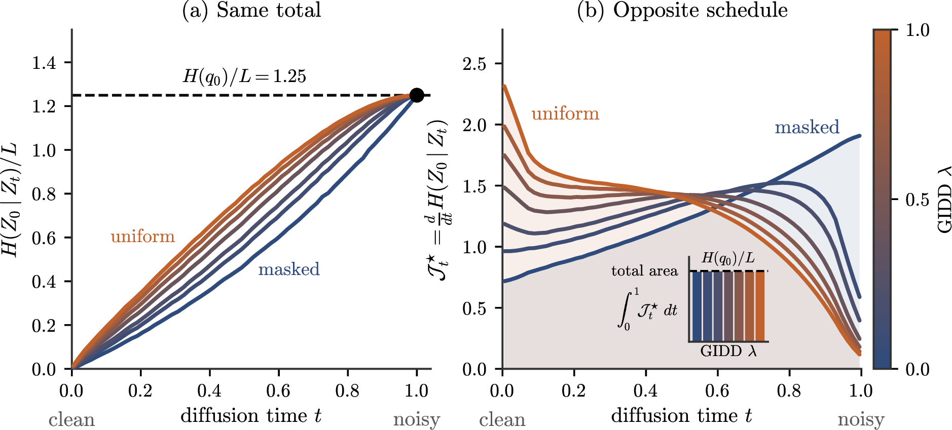
The entropy constant in 4 is not mere bookkeeping; it has a precise information-theoretic origin. Evaluated at the oracle reverse rate \(\widehat{Q}_t\), the per-time ELBO cost that remains is exactly the rate at which the forward process destroys information about the data, \[\mathcal{J}^\star_t :=\mathbb{E}_{Z_0,Z_t}\!\left[\sum_{y\neq Z_t}\Phi\!\left(\widehat{Q}_t(Z_t,y\mid Z_0),\widehat{Q}_t(Z_t,y)\right)\right] =\frac{d}{dt}H(Z_0\mid Z_t) =-\frac{d}{dt}I(Z_0;Z_t)\ge0,\] the CTMC counterpart of the I-MMSE relation between estimation and information (Theorem 4, §5.1). Integrated over the schedule this telescopes to the total information the data carries, the data entropy \(H(Z_0)=H(p_{\mathrm{data}})\) (Figure 2).
2.1.0.8 A Pythagorean split.
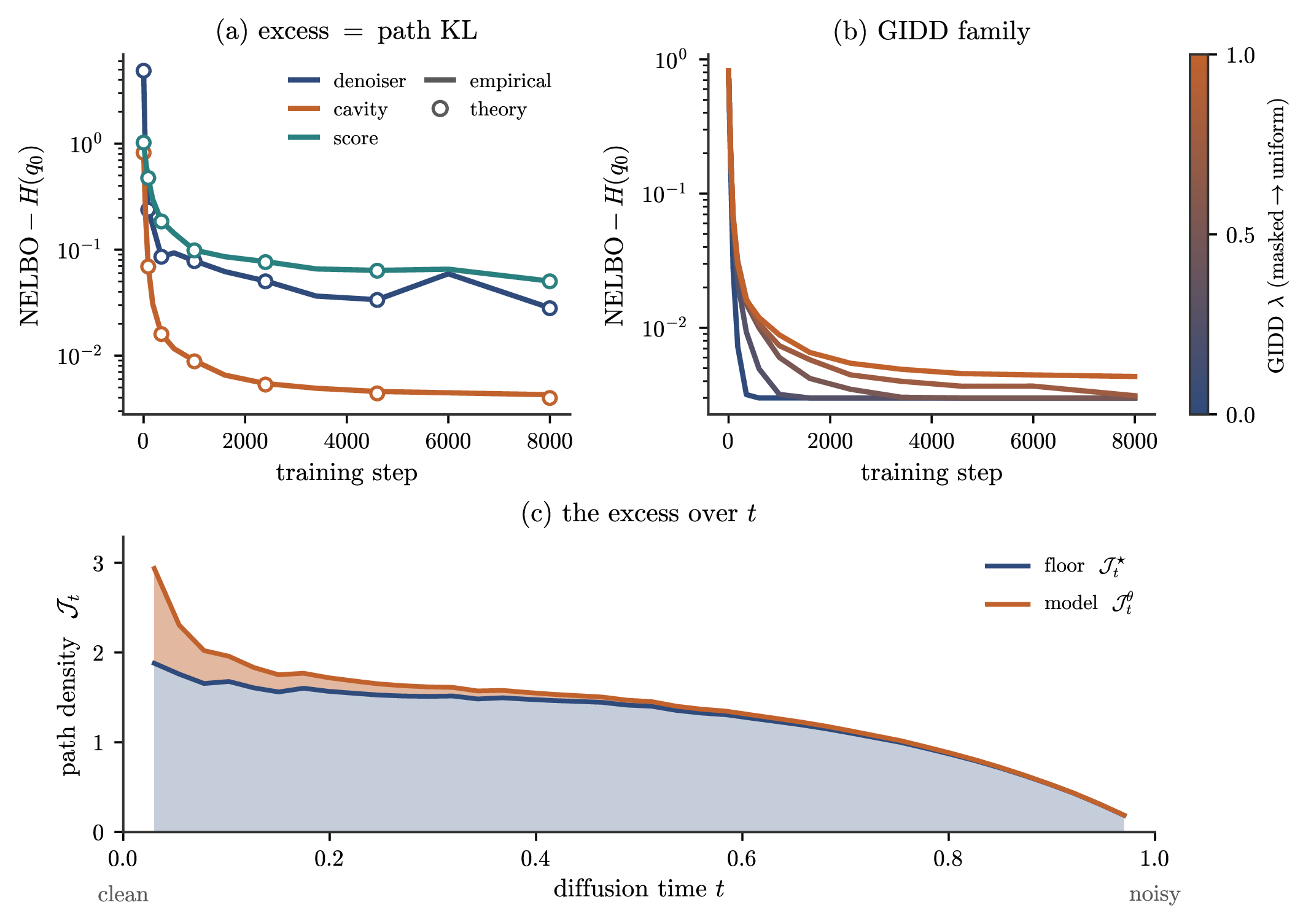
The two previous facts combine into a proof of the Oracle Distance 4 . For any model rate, the per-time trained cost separates exactly, with no cross term, into what the oracle pays plus how far the model’s rates are from the oracle’s (a Bregman property of \(\Phi\); Proposition 2, §5.1): \[\underbrace{\mathbb{E}_{Z_0,Z_t}\!\left[\textstyle\sum_{y\ne Z_t}\Phi\big(\widehat{Q}_t(Z_t,y\mid Z_0),\widehat{Q}^\theta_t(Z_t,y)\big)\right]}_{\text{trained cost}} = \underbrace{\;\mathcal{J}^\star_t\;}_{\text{oracle cost}} + \underbrace{\mathbb{E}_{Z_t}\!\left[\textstyle\sum_{y\ne Z_t}\Phi\big(\widehat{Q}_t(Z_t,y),\widehat{Q}^\theta_t(Z_t,y)\big)\right]}_{\text{model--oracle rate divergence}}.\] Integrating over time, the oracle cost telescopes to the data entropy \(H(q_0)\) by the information-loss identity above, while the model–oracle divergence accumulates into the path KL: this is the identity.
2.1.0.9 A universal entropy floor.
The same result also identifies the intrinsic floor of the ELBO. Since the path-law KL in 4 is non-negative and vanishes exactly at the true marginal reverse dynamics, for a model class expressive enough to realize them, we get \[\label{eq:elbo-floor-intro} \boxed{\; \inf_{\theta}\;-\mathbb{E}_{q_0}\!\left[\mathop{\mathrm{ELBO}}_{[0,T]}(\theta;\, z_0)\right] = H(p_{\mathrm{data}}). \;}\tag{7}\] Thus the best achievable value is not an artifact of the particular noising process or parameterization; it is the data entropy (Figure 3). Lemma 3 and Corollary 3 (§5.4) give the formal statements, and Figure 7 shows the boundary-term decomposition summing to this floor. The ELBO has a universal entropy floor, and the excess above that floor measures pathwise mismatch to the true reverse process.
2.1.0.10 Training clocks and the information-uniform time.
In practice the path integral in 3 is estimated by Monte Carlo over \(t\) and \(z_t\sim q_{t\mid 0}(\cdot\mid z_0)\), optionally with an importance density \(p_{\mathrm{IS}}(t)\) for variance reduction; choosing \(p_{\mathrm{IS}}\) is the same as choosing the clock on which the reverse chain is run (§4.4). Beyond the variance-optimal choice, one clock is intrinsic to the process: since the oracle cost rate is \(\mathcal{J}^\star_t=\tfrac{d}{dt}H(Z_0\mid Z_t)\) (Theorem 4), the clock \(\tau(t)=H(Z_0\mid Z_t)/H(q_0)\) drains information linearly, \(I(Z_0;Z_\tau)=(1-\tau)\,H(q_0)\), and straightens the otherwise process-dependent curves of Figure 2a onto a single diagonal.
2.2 Discrete diffusion for sequential data↩︎
Discrete diffusion is most often applied to sequence modeling, broadly any multi-dimensional data such as text, images, music, or graphs. However, a practitioner immediately meets three apparently different ways to parameterize the model: predict the clean token directly (a denoiser); the bridge plug-in trick, widely assumed to be an equivalent way of training that same denoiser (it is not); or predict a ratio of noisy conditionals (a concrete score). Folklore holds that some of these mysteriously misbehave, and indeed the uniform-diffusion ELBO can diverge at initialization. This section resolves the confusion with the central guiding principle we just introduced in the previous section: all three are coordinates of one object, the true reverse rate that the ELBO optimizes. Choosing a parameterization is just choosing which coordinates of that object to learn.
Using this one fact we give an answer to several open practical questions: what is the dictionary that converts between the three parameterizations, why a denoiser model fed to a cavity sampler silently trains a different law under uniform but not masked diffusion, what it would take to improve on masked diffusion, and it also provides calibration checks that run at initialization, among others.
2.2.0.1 Sequences as product spaces.
Sequential data lives on a product space (§6), whose (high-order) positional correlations are exactly the structure generative models aim to capture. We index the \(L\) positions by \(1\le i\le L\) and work on the finite product state space \[\mathcal{X}:=\mathcal{X}_1\times\cdots\times \mathcal{X}_L.\] To exploit this structure, the standard choice is a noising process that factors across positions (Theorem 6, §6.1): each position is corrupted independently, so for times \(s<t\) the forward kernel is \[q_{t\mid s}(y\mid x):=\prod_{i=1}^L q_{t\mid s}^i(y^i\mid x^i), \qquad x,y\in\mathcal{X},\] where \(x^i\) is the \(i\)-th coordinate, \(x^{-i}:=(x^j)_{j\neq i}\) the remaining coordinates, and \(q_{t\mid s}^i\) the forward kernel on \(\mathcal{X}_i\). Equivalently, by the Kolmogorov forward equation, the generator factors additively, \[Q_t(x,y) = \sum_{i=1}^L (Q_t)_i(x,y), \qquad (Q_t)_i(x,y) = \mathbf{1}\{x^{-i}=y^{-i}\}\,R_t^i(x^i,y^i), \label{eq:walkthrough-generator-factorization}\tag{8}\] so jumps occur one coordinate at a time, at a rate \(R_t^i\). Nothing forces the per-position processes to be equal, though they usually are.
This factorization into token-wise jump rates is what makes both training and the standard marginal-based sampling tractable, as we now show. Like the left-to-right factorization of autoregressive models, this choice trades a (hopefully mild) loss of expressivity for tractability.
2.2.0.2 From sequence rates to token rates.
The payoff of factorization is that the whole reverse process is fixed by token marginals alone, never full-sequence laws. To see it, we compute the true reverse rate of Theorem 5 for the clean-conditioned positional rates, averaging over \(q(z_0\mid z_t)\), and cancelling the non-\(i\) factors, to get \[(\widehat{Q}_t)_i(z_t, y) = \mathbb{E}_{}\!\left[(\widehat{Q}_t)_i(Z_t, y\mid Z_0) \;\middle|\; Z_t=z_t\right] = R_t^i(y^i,z_t^i)\, \mathbb{E}_{q(z_0^i\mid z_t)}\!\left[\frac{q^i_{t\mid 0}(y^i\mid z_0^i)}{q^i_{t\mid 0}(z_t^i\mid z_0^i)}\right]. \label{eq:walkthrough-rates-through-marginal-denoiser}\tag{9}\] The reverse rates therefore depend on the data only through the clean-token marginals \(q(z_0^i\mid z_t)\), which is our first key insight for sequence modeling and is formalized as the denoiser coordinate in Theorem 7 (§6). The literature typically posits a token-level parameterization on the strength of factorizability; deriving it through the projection result instead shows what that factorization buys (the dependence on data through those clean-token marginals alone) and thereby which token-level choices affect the optimized law and which are immaterial.
2.2.0.3 Existing parameterizations and open questions.
The marginal \(q(z_0^i\mid z_t)\) is the familiar denoiser, which we denote by \(\pi_i^\star\): the \(i\)-th clean-token law given the current noisy sequence, \[\boxed{\;\pi_i^\star(z_0^i\mid z_t,t) := q(z_0^i\mid z_t).\;}\] The standard recipe, known as the mean parameterization, fits a neural network head \(\pi_i^\theta\approx\pi_i^\star\), plugs it into 9 to obtain rates \(\widehat{Q}_t^\theta\), and feeds those to the ELBO of Theorem 1; it is commonly read as the “average reverse rate” under the denoiser’s uncertainty. Reverse sampling then factors the step through the same head, \[p_{s\mid t}^\theta(z_s\mid z_t) = \prod_{i=1}^L p^\theta(z_s^i\mid z_t), \qquad p^\theta(z_s^i\mid z_t) = \mathbb{E}_{\pi_i^\theta(z_0^i\mid z_t,t)}\!\left[q^i_{s\mid t,0}(z_s^i\mid z_t^i, z_0^i)\right], \label{eq:walkthrough-ancestral-sampling-marginal}\tag{10}\] even though the true law \(q_{s\mid t}\) cannot factor over positions: if it did, the clean-data law \(q(z_0)=q(z_0\mid z_T)\) (by terminal mixing, Assumption 1) would factor too, giving a pure unigram model.
This recipe works for masked diffusion but fails for uniform diffusion, where the ELBO diverges at initialization. Uniform-diffusion (UDM) and generalized-interpolating (GIDD) works instead adopt the bridge plug-in parameterization, in which the forward kernel \(q_{t\mid 0}^i\) is averaged over the network’s output distribution before forming the rate 1 , and surprisingly this keeps the ELBO finite and allows smooth training. A third route, that of concrete scores, instead reads the head as ratios of noisy conditional laws. These options raise the central questions we answer next: how are the three related, are they interchangeable, why does one of them sometimes fail, and what reverse CTMC does each actually induce?
2.2.0.4 Three coordinates, one object.
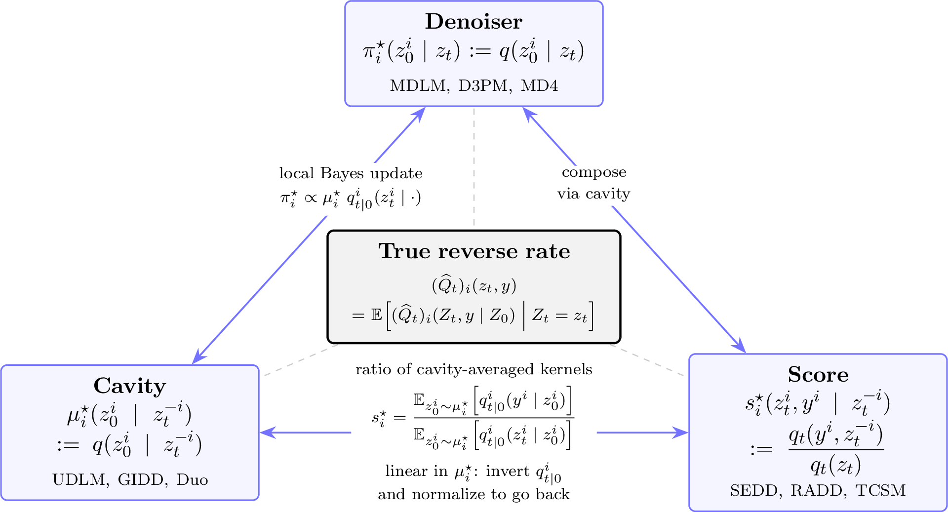
The answer lies in the ELBO’s unique optimizer, the unconditional reverse rate of Theorem 5, because we can rewrite 9 in terms of true laws other than the denoiser. The bridge plug-in turns out to target the cavity law \(\mu_i^\star\), namely the \(i\)-th clean-token law given the context \(z_t^{-i}\) but ignoring its own noisy observation \(z_t^i\), \[\boxed{\;\mu_i^\star(z_0^i\mid z_t^{-i},t) := q(z_0^i\mid z_t^{-i}),\;}\] while the concrete score \(s_i^\star\) targets a ratio of noisy conditional laws, \[\boxed{\;s_i^\star(z_t^i,y^i\mid z_t^{-i},t) := \frac{q_t(y^i, z_t^{-i})}{q_t(z_t)},\;}\] where \((y^i,z_t^{-i})\) denotes the sequence \(z_t\) with its \(i\)-th token replaced by \(y^i\). Our second contribution makes this picture exact by identifying three exact and equivalent expressions for the token-wise true reverse rates \((\widehat{Q}_t)_i\), which together form a coordinate dictionary, \[\begin{align} (\widehat{Q}_t)_i(z_t,y) & = R_t^i(y^i,z_t^i)\, \mathbb{E}_{\pi_i^\star(\cdot\mid z_t,t)}\!\left[\frac{q_{t\mid 0}^i(y^i\mid\cdot)}{q_{t\mid 0}^i(z_t^i\mid\cdot)}\right] & & \text{\eqref{eq:denoiser-parameterization-oracle}, denoiser} \\ & = R_t^i(y^i,z_t^i)\, \frac{\mathbb{E}_{\mu_i^\star(\cdot\mid z_t^{-i},t)}\!\left[q_{t\mid 0}^i(y^i\mid\cdot)\right]}{\mathbb{E}_{\mu_i^\star(\cdot\mid z_t^{-i},t)}\!\left[q_{t\mid 0}^i(z_t^i\mid\cdot)\right]} & & \text{\eqref{eq:cavity-parameterization-oracle}, cavity} \\ & = R_t^i(y^i,z_t^i)\,s_i^\star(z_t^i,y^i\mid z_t^{-i},t) & & \text{\eqref{eq:score-parameterization-oracle}, score.} \end{align}\] To read these off: the denoiser line averages the forward-kernel ratio \(q_{t\mid 0}^i(y^i\mid\cdot)/q_{t\mid 0}^i(z_t^i\mid\cdot)\) over the clean token \(z_0^i\sim\pi_i^\star\); the cavity line takes a ratio of the cavity-averaged kernels \(\mathbb{E}_{\mu_i^\star}\!\left[q_{t\mid 0}^i(\cdot\mid z_0^i)\right]\); and the score is already that reweighting and enters raw. All three agree at the oracle laws, which is exactly the dictionary. But averaging the ratio (denoiser) and taking the ratio of averages (cavity) are different operations on a learned head, which is why the denoiser/cavity distinction bites for uniform yet vanishes for masked diffusion (next paragraph).
Fitting a head to each yields a different parameterization, and each is a complete specification of the generative process, since substituting a coordinate into the rate fixes the reverse jump rates and, by the Kolmogorov forward equation, those rates in turn determine the reverse CTMC in full. Figure 4 gathers the three coordinates: the oracle law each one learns, the literature methods it recovers, and the closed-form conversions between them.
Because all three coordinates target the same oracle object, namely the unique optimum of the ELBO, each head \(\pi_i^\theta,\mu_i^\theta,s_i^\theta\) is optimized exactly at \(\pi_i^\star,\mu_i^\star,s_i^\star\), uniquely up to identifiability of the head-to-rate map.
2.2.0.5 Why masked diffusion is special.
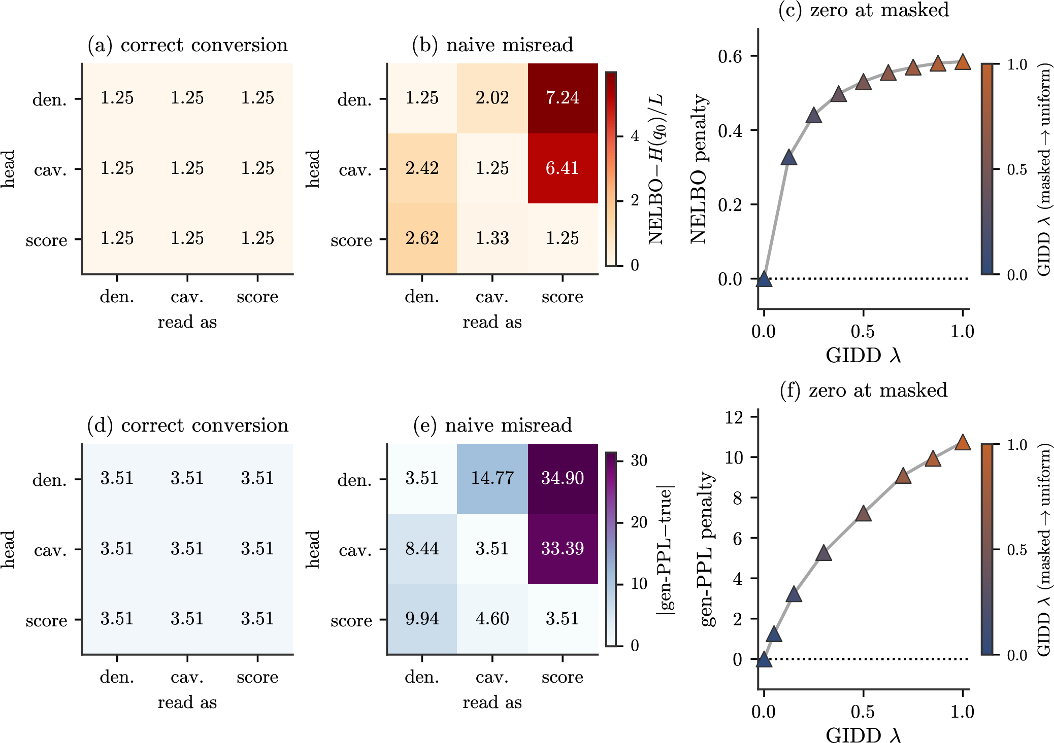
The link between \(\pi_i^\star\) and \(\mu_i^\star\) is simple: the denoiser is the cavity reweighted by the local forward kernel \(q_{t\mid 0}^i(z_t^i\mid z_0^i)\), \[\pi_i^\star(z_0^i \mid z_t,t) \propto \mu_i^\star(z_0^i\mid z_t^{-i},t)\,q_{t\mid 0}^i(z_t^i\mid z_0^i).\] Thus, the forward kernel \(q_{t\mid 0}^i(z_t^i\mid z_0^i)\) is exactly the Bayes update for observing the local token \(z_t^i\) on top of the context \(z_t^{-i}\). This splits the mutual information between \(z_0^i\) and \(z_t\) into two parts: what the context \(z_t^{-i}\) reveals (the cavity \(\mu_i^\star\), which must be learned), and what the local token \(z_t^i\) adds (the forward kernel weight, available analytically). A denoiser head must reproduce both of these, which is a concrete source of its training difficulty. Masked diffusion escapes the distinction entirely, because at a masked token the local observation is uninformative and thus \(q_{t\mid 0}^i(\mathfrak{m}\mid\cdot)\) constant, so that \(\pi_i^\star=\mu_i^\star\), that is, the denoiser and cavity coincide in masked diffusion (Corollary 4, §7). We show the importance of this distinction in Figure 5.
2.2.0.6 Two sources of modeling bias.
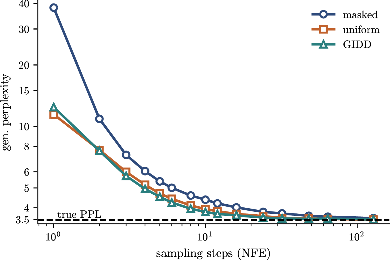
The framework cleanly separates the two sources of error in a discrete-diffusion model. The first is reverse-rate error, the gap between the model rate and the true reverse jump rate, which is exactly what the ELBO measures, by the Oracle Distance Theorem 3. The second is sampling factorization error and is invisible to the ELBO. The trajectory drift noted above is not a third source: it is the same reverse-rate error, incurred now at the model’s own self-generated states rather than at the true (teacher-forced) states the ELBO scores; in the well-specified, sufficient-capacity limit the learned rate is correct at every state and no drift occurs, so drift is a generalization gap rather than an objective mismatch (§9). Factorization error, by contrast, persists even when the reverse-rate error is exactly zero. The literature uses various small-time sampling schemes (Euler, \(\tau\)-leaping, Tweedie), but rarely makes the sequence-to-token derivation explicit, even though the sampling gap is exactly the factorization bias. All such schemes rest on the same fact, namely that over a short step \([s,t]\) the rates \((\widehat{Q}_t)_i(z_t,y)\) can be treated as constant up to \(O(t-s)\) terms, and under that approximation the unconditional reverse rate factors exactly, so the factorized ancestral sampler is justified. Figure 6 isolates this factorization error: even an oracle with zero reverse-rate error degrades at few-step sampling.
2.2.0.7 Calibration at initialization.
The framework also yields calibration identities at initialization, for an uninformative head \(1/V\). First, a cavity \(1/V\) head has per-token NELBO \(\log V\) (Proposition 4, §6), which provides a useful debugging tool, whereas a denoiser \(1/V\) head instead makes the uniform-diffusion NELBO diverge (Proposition 6, §7); both identities are confirmed numerically in Figure 7. This divergence also pinpoints when denoisers are hard to train: whenever placing mass on the “wrong” token near the clean endpoint \(t_1\) creates singular quotients \(q^i_{t\mid 0}(y^i\mid z_0^i)/q^i_{t\mid 0}(z_t^i\mid z_0^i)\), which is precisely UDM’s failure mode.
![Figure 7: (a) A cavity head \mu_i^\theta\equiv1/V has per-token NELBO \log V once boundary terms are kept (Proposition 4). (b) The same head read as a denoiser makes the uniform NELBO diverge, linearly in \log(1/\beta_{t_1}) with slope \tfrac{V-1}{V} (Proposition 6), while masked stays finite. (c) The oracle NELBO splits as reconstruction + path + terminal prior, summing to the same H(q_0) for any noising process (Corollary 3; the window [0.1,0.9] exaggerates the boundary terms).](/article/2607.05381/figures/fig_calibration.png "fig:")
2.2.0.8 Practical takeaways.
The framework reduces to a few concrete rules for the practitioner.
Match the neural network head during sampling to its training loss, or convert. A head is optimized by the law its loss targets; feed a cavity head into a denoiser sampler and one is missing the analytic Bayes update 39 .
Avoid a raw denoiser head for uniform and GIDD. Its ELBO diverges at initialization (Proposition 6); use the cavity (bridge plug-in) coordinate, which stays finite and well-calibrated.
Use the \(\log V\) identity as a calibration and debugging tool. A cavity \(1/V\) head has per-token NELBO \(\log V\) independently of the diffusion process and the training endpoints \([t_1,t_2]\), after including the boundary terms.
Keep the boundary terms. The reconstruction and terminal-prior KL terms are required for ELBOs to be comparable across processes; dropping them, as is common, silently breaks such comparisons.
2.2.0.9 Instantiations: masked, uniform, GIDD.
Section §7 instantiates the framework on the three standard processes. We do so by showing that GIDD’s ELBO is really a generic cavity ELBO, valid for any source-independent rate, with a closed-form integrand given by a KL plus an Itakura–Saito term (Proposition 5). Specializing it recovers the masked, uniform, and GIDD integrands, and the score coordinate likewise re-derives the results of SEDD and RADD in a few steps; the cavity optimality of the UDM bridge plug-in observed by [10] follows as one special case (see §3). Table ¿tbl:tab:process-summary? collects the resulting formulas, including the prior boundary terms that are usually dropped in the literature but are needed to compare ELBOs across methods.
3 Background and related work↩︎
3.0.0.1 Discrete diffusion and its continuous-time form.
Discrete diffusion originates with multinomial and structured categorical corruption processes [1], [2], the discrete analogue of the Gaussian diffusion line [11], [12], and now scales to large language models [13]. Campbell et al. [3] cast discrete diffusion as a continuous-time Markov chain (CTMC) with exact forward and reverse rates and a continuous-time variational bound, later extended by score-based [4], [14] and flow-based [15], [16] formulations, and generalized to broad classes of Markov processes by denoising Markov models [17] and Generator Matching [18]. Section §4 is a self-contained re-derivation of the CTMC ELBO building on [3], with the reconstruction and terminal-prior boundary terms and the rate-support and regularity conditions made explicit, and with two derivations (an infinitesimal-KL argument and a Girsanov argument, Theorem 2). Existing discrete formulations absorb the boundary terms into model-independent constants or send them to zero with \(T\to\infty\) [3]–[5], [19], which makes reported ELBOs incomparable across noising processes as implemented; we keep them explicit throughout, which is what enables the cross-process calibration results of §6. To our knowledge, no discrete-diffusion work states the exact identity, with boundary terms, for arbitrary model rates. Other insights from our framework, such as the equivalence between importance sampling and the process’ time parameterization, connect to likelihood-faithful versus reweighted diffusion objectives [20]–[23].
3.0.0.2 Reverse-process parameterizations.
The learned reverse process is parameterized in several ways: as a denoiser [1]–[3], [5], [9], as a concrete score [4], [14], [24]–[26], or as a leave-one-out or cavity law [6], [10], [27]–[29], with the masked ELBO reducing to weighted cross-entropy [5], [9], [30]. Two recent frameworks unify subsets of these: Generator Matching [18] regresses a marginal Markov-process generator, and Target Concrete Score Matching [26] unifies training objectives through the target concrete score, recovering several existing masked and score-based objectives as special cases. Generator Matching in particular already contains, at the level of matching objectives, two ingredients we use: the marginal generator as a posterior average of conditional generators, and Bregman divergences as the loss class whose conditional and marginal forms share gradients (their Propositions 1–2). What it does not provide that we do is the likelihood side: the exact CTMC NELBO, boundary terms included, is such a Bregman objective for \(\Phi\), so the projection optimum is the maximum-ELBO reverse process, the excess above the oracle is a path KL, and the irreducible part is the information-destruction rate. Section §6 is complementary at the parameterization level: rather than a single objective, we give an explicit coordinate dictionary of the reverse rate for all denoiser, cavity, and score parameterizations, with exact conversion formulas, and identify which coordinate each literature loss optimizes. Prior work often blurs the position- versus sequence-level distinction and reads one network in another’s sampler without converting, the score line [4], [25] and the independent uniform-diffusion analysis of [10] being the closest exceptions.
3.0.0.3 The denoiser-versus-leave-one-out distinction.
Concurrently and independently, Gourevitch et al. [10] have recently observed for the special case of uniform diffusion (UDM) that the bridge plug-in is optimized by a leave-one-out (cavity) law rather than the standard denoiser, deriving denoiser/leave-one-out/score conversions for UDM that they use to improve UDM training and sampling. Our work obtains this result by a different route that places it within a general product-CTMC treatment. The Oracle Distance Theorem 3 and the reverse-rate projection it induces characterize the denoiser, cavity, and score optima, and their conversion formulas, for every token-factorizable noising process from a single projection principle. Our framework also explains exactly when and why the coordinates differ and when a denoiser parameterization makes the ELBO ill-posed, with explicit divergence rates for UDM (Proposition 6) that give a theoretical account of the leave-one-out advantage that Gourevitch et al.document empirically. Furthermore, their empirical gains on text modelling provide strong evidence that distinctions such as the exact reverse-rate process and oracle law being optimized are far from purely academic and have a measurable effect on discrete diffusion modeling.
3.0.0.4 Information-theoretic view.
The irreducible ELBO cost we identify with \(\tfrac{d}{dt}H(Z_0\mid Z_t)=-\tfrac{d}{dt}I(Z_0; Z_t)\) is the CTMC instance of estimation–information identities: the Gaussian I-MMSE relation [31], its jump-rate analogue whose natural loss is exactly our jump divergence \(\Phi\) [32], the information-theoretic reading of the continuous diffusion ELBO [33], and the discrete I-MDSE/I-MDCE relations of [19], which they state at the oracle in the score coordinate for general rate matrices and in the cross-entropy coordinate for masked diffusion, with \(T\to\infty\). Our identities extend the latter along three axes: from the oracle to arbitrary model rates (the excess being exactly a path KL), to every coordinate of any token-factorizable process, and to finite windows with explicit boundary terms. The conditional-mean optimality and Pythagorean decomposition are special cases of [34], the jump-rate counterpart of the denoiser/cavity/score identities in continuous diffusion [35]. Because squared error is itself the Bregman divergence of \(F(u)=\tfrac12\|u\|^2\) and \(\Phi\) that of \(F(u)=u\log u-u\), these identities are not merely parallel: the Gaussian I-MMSE and our CTMC case are two instances of one Bregman representation of the information loss.
4 A continuous-time discrete diffusion framework↩︎
The proofs in this and the following sections follow one recurring pattern: identify the exact reverse Markov process, then ask what part of it a model can represent. The variational step to deduce the ELBO bound is standard after realizing that a diffusion model is a VAE whose latent is the noising trajectory; in continuous time the discrete sum of bridge-kernel KLs becomes a path integral of local jump-rate divergences \(\Phi(\widehat{Q}_t(z_t,y\mid z_0),\widehat{Q}_t^\theta(z_t,y))\), plus a reconstruction term at the lower endpoint and a terminal-prior term at the upper endpoint. This is the CTMC ELBO of Section §4.3, obtained either as a vanishing-mesh limit of the discrete-time ELBO or directly as the relative entropy between jump processes using Girsanov’s formula.
The true bridge rate still depends on the hidden clean data \(Z_0\), whereas the learned reverse CTMC sees only the noisy state \(Z_t\). The ELBO therefore poses a local projection problem, whose minimizer among \(Z_t\)-measurable rates is the posterior mean of the clean-conditioned rate: the marginal time-reversal of the forward process. Its oracle per-time ELBO cost is exactly the information the forward process destroys, \(\tfrac{d}{dt}H(Z_0\mid Z_t)\), and the Bregman–Pythagoras identity for \(\Phi\) splits any model’s path cost into this irreducible term plus its mismatch to the oracle rate. With the two boundary terms, this yields the main result of Section §5: after subtracting the fixed data entropy \(H(q_0)\) and up to the two endpoint terms, the negative ELBO (NELBO) is exactly the path-law KL from the oracle reverse CTMC to the learned one.
The final sequence-modeling sections §§6–7 specialize this identity. For product noising processes, the forward generator changes one token at a time, so the oracle reverse rate decomposes into one-token jumps, expressible in three coordinates: a denoiser, a cavity law, or a concrete score.
4.1 Variational formulation of diffusion models↩︎
We begin with the variational identity underlying VAEs. Let \(p^\theta(z_0,z_1)\) be a generative model for a finite data distribution \(z_0\sim q_0\) on \(\mathcal{X}\) and a latent variable \(z_1\in\mathcal{Z}\). Let \(q(z_1\mid z_0)\) be an encoder satisfying \(q(z_1\mid z_0) \ll p^\theta(z_0,\cdot)\) for every \(z_0\).
The standard ELBO derivation starts from the marginal log-likelihood and applies Jensen’s inequality for the concave function \(\log\): \[\log p^\theta_0(z_0) = \log \mathbb{E}_{q(z_1\mid z_0)}\!\left[\frac{p^\theta(z_0,z_1)}{q(z_1\mid z_0)}\right] \geq \mathbb{E}_{q(z_1\mid z_0)}\!\left[\log \frac{p^\theta(z_0,z_1)}{q(z_1\mid z_0)}\right] := \mathop{\mathrm{ELBO}}(\theta;\, z_0). \label{eq:VAE-ELBO-def}\tag{11}\] The right-hand side is the evidence lower bound, which can be split as \[\mathop{\mathrm{ELBO}}(\theta;\, z_0) = \mathbb{E}_{q(z_1\mid z_0)}\!\left[\log p^\theta(z_0\mid z_1)\right] - \mathop{\mathrm{KL}}\!\left(q(\cdot\mid z_0)\,\middle\|\,p_{z_1}^\theta\right).\] The two terms are the reconstruction log-likelihood and prior KL, respectively. Alternatively, the ELBO can be derived via the data processing inequality \[\begin{align} \log q_0(z_0)-\mathop{\mathrm{ELBO}}(\theta;\, z_0) & = \mathbb{E}_{q_{1\mid 0}(z_1\mid z_0)}\!\left[\log \frac{q(z_0, z_1)}{p^\theta(z_0, z_1)}\right] \\ & = \mathop{\mathrm{KL}}\!\left(q(\cdot\mid z_0)\,\middle\|\,p^\theta(\cdot\mid z_0)\right) + \log q_0(z_0) - \log p^\theta_0(z_0) \\ & \ge \log q_0(z_0) - \log p^\theta_0(z_0). \end{align}\] In particular, this shows that the gap in the ELBO inequality is exactly a KL divergence: \[\begin{align} \log p^\theta_0(z_0)-\mathop{\mathrm{ELBO}}(\theta;\, z_0) & = \mathop{\mathrm{KL}}\!\left(q(\cdot\mid z_0)\,\middle\|\,p^\theta(\cdot\mid z_0)\right) \geq 0. \end{align}\] It measures the discrepancy between the encoding and model posterior latent laws.
Diffusion models are VAEs whose latent variable is the noising trajectory. Fix \(z_0\in\mathcal{X}\) and let \(z_{0:N}\) be a discrete-time Markov trajectory with \(N\geq1\), initial law \(q_0\), and forward kernels \(q_{t\mid t-1}\). Then \[q_{1:N\mid 0}(z_{1:N}\mid z_0) = \prod_{t=1}^N q_{t\mid t-1}(z_t\mid z_{t-1}).\] The learned reverse-time model factors as \[p^\theta(z_{0:N}) = p^\theta_N(z_N) \prod_{t=1}^N p^\theta_{t-1\mid t}(z_{t-1}\mid z_t),\] and is also Markov in forward time. In the VAE interpretation, \(z_{1:N}\) is the latent variable and \(p^\theta_N\) is its terminal prior.
Proposition 1 (Discrete-time diffusion ELBO). Assume the KL terms below are well defined. Then \[\begin{align} \mathop{\mathrm{ELBO}}(\theta;\, z_0) & = \mathbb{E}_{q_{1\mid 0}(z_1\mid z_0)} \left[ \log p^\theta_{0\mid 1}(z_0\mid z_1) \right] - \mathop{\mathrm{KL}}\!\left(q_{N\mid 0}(\cdot\mid z_0)\,\middle\|\,p^\theta_N\right) \nonumber \\ & \qquad - \sum_{t=2}^N \mathbb{E}_{q_{t\mid 0}(z_t\mid z_0)} \left[ \mathop{\mathrm{KL}}\!\left(q_{t-1\mid t,0}(\cdot\mid z_t,z_0)\,\middle\|\,p^\theta_{t-1\mid t}(\cdot\mid z_t)\right) \right]. \label{eq:discrete-time-diffusion-elbo} \end{align}\qquad{(1)}\] Moreover, \[\log p^\theta_0(z_0)-\mathop{\mathrm{ELBO}}(\theta;\, z_0) = \mathop{\mathrm{KL}}\!\left(q_{1:N\mid 0}(\cdot\mid z_0)\,\middle\|\,p^\theta_{1:N\mid 0}(\cdot\mid z_0)\right) \geq 0.\]
Proof. We start with the VAE ELBO equality with latent variable \(z_{1:N}\) and use the reverse-model factorization above together with the reverse factorization \[q_{1:N\mid 0}(z_{1:N}\mid z_0) = q_{N\mid 0}(z_N\mid z_0) \prod_{t=2}^N q_{t-1\mid t,0}(z_{t-1}\mid z_t,z_0)\] to obtain \[\begin{align} \mathop{\mathrm{ELBO}}(\theta;\, z_0) & = \mathbb{E}_{q_{1:N\mid 0}(z_{1:N}\mid z_0)}\left[ \log \frac{ p^\theta(z_{0:N}) }{ q_{1:N\mid 0}(z_{1:N}\mid z_0) } \right] \nonumber \\ & = \mathbb{E}_{q_{1:N\mid 0}(z_{1:N}\mid z_0)} \left[ \log \frac{ p^\theta_N(z_N) \prod_{t=1}^{N}p^\theta_{t-1\mid t}(z_{t-1}\mid z_t) }{ q_{N\mid 0}(z_N\mid z_0) \prod_{t=2}^{N}q_{t-1\mid t,0}(z_{t-1}\mid z_t,z_0) } \right] \nonumber. \end{align}\]
Splitting the logarithm into boundary and transition terms gives ?? . The gap identity is the corresponding VAE identity with latent variable \(z_{1:N}\). ◻
4.2 CTMC formulation↩︎
We now specialize the trajectory latent to a continuous-time Markov chain; see [36]–[38] for standard textbook references.
4.2.0.1 Notation.
A single letter \(q\) or \(p\) denotes the finite-dimensional marginals, kernels, and bridges of a process, with subscripts recording the relevant times: \(q_t\) is the time-\(t\) marginal, \(q_{t\mid s}\) the transition kernel for times \(s<t\), \(q_{t\mid 0}(\cdot\mid z_0)\) the forward kernel from clean data, and \(q_{s\mid t,0}(\cdot\mid z_t,z_0)\) the bridge. We often identify a random variable with its value and drop the event when it is clear, writing \(q(z_0\mid z_t)\) for \(q(Z_0=z_0\mid Z_t=z_t)\). Jump rates take \(Q,R\), and sometimes \(a,b\): \(Q_t\) is the forward generator, a hat \(\widehat{Q}_t\) denotes time reversal.
We abbreviate “almost every” and “almost surely” for a probability measure \(\mu\) as \(\mu\)-a.e.and \(\mu\)-a.s., for properties that hold on a set of probability 1. For two laws \(\mu,\nu\), absolute continuity \(\mu\ll\nu\) means \(\nu(A)=0\Rightarrow\mu(A)=0\). On finite state spaces this is simply support inclusion \(\mathop{\mathrm{supp}}\mu\subseteq\mathop{\mathrm{supp}}\nu\), and the associated relative density (the Radon–Nikodym derivative) \(d\mu/d\nu\) is the likelihood ratio. We use \(H(Z)=-\sum_z p(z)\log p(z)\) for the entropy of a discrete variable \(Z\) and \(I(X;Y)=\mathop{\mathrm{KL}}\!\left(p_{X,Y}\,\middle\|\,p_X p_Y\right)=H(X)-H(X\mid Y)\) for the mutual information between \(X\) and \(Y\).
4.2.0.2 CTMC processes and their generators.
Let \(\mathcal{X}\) be finite and \(0<T\), possibly \(T=\infty\). A continuous-time discrete diffusion is a continuous-time Markov chain (CTMC) \((Z_t)_{t\in[0,T]}\) on \(\mathcal{X}\) whose law is fixed by a time-dependent rate matrix (generator) \(Q_t\), with \[Q_t(x,y)\geq 0\;\;(x\neq y), \qquad Q_t(x,x) = -\sum_{y\neq x}Q_t(x,y),\] so that each row sums to zero. The off-diagonal entry \(Q_t(x,y)\) is the instantaneous rate of the jump \(x\to y\): the transition kernel \[q_{t\mid s}(y\mid x)=\mathbb{P}(Z_t=y\mid Z_s=x)\] satisfies, as \(h\downarrow0\), \[q_{t+h\mid t}(y\mid x) = \delta(x,y) + h\,Q_t(x,y) + o(h).\] While the chain is in a given state \(x\), the time until the next jump is exponentially distributed with rate \(-Q_t(x,x)\), i.e., \(\mathbb{P}(Z_t=x,\;\forall t\in[s,u]\mid Z_{s}=x) = \exp(\int_{s}^{u} Q_t(x,x)\,dt)\). Conditional on a jump from \(x\) occurring at time \(t\), the probability of destination \(y\ne x\) is proportional to \(Q_t(x,y)\), i.e., \(\mathbb{P}(Z_{t+} = y\mid Z_t = x, Z_{t+} \ne x) = Q_t(x,y)/(-Q_t(x,x))\). Sample paths are right-continuous and piecewise constant.
4.2.0.3 Kolmogorov equations.
Arranged as matrices with normalized rows, the kernels obey Chapman–Kolmogorov \(q_{u\mid s}=q_{t\mid s}q_{u\mid t}\) and the forward and backward linear ODEs \[\partial_t q_{t\mid s}=q_{t\mid s}Q_t,\qquad \partial_s q_{t\mid s}=-Q_s q_{t\mid s},\qquad q_{s\mid s}=I.\] In particular, with \(q_0\) given, the marginal \(q_t\) solves \(\partial_t q_t=q_t Q_t\), that is, \(\partial_t q_t(y)=\sum_x q_t(x)Q_t(x,y)\). By the uniqueness of solutions for ODEs with initial condition, the law of the chain is uniquely determined by \(q_0\) and \(Q_t\).
4.2.0.4 Path laws and trajectory likelihoods.
Three standard facts, used in the Girsanov derivation of §4.3, describe the process at the path level; see [36]–[38]. The first is well-posedness: a law at the time from which the process is run (the left endpoint for a forward chain, the right endpoint for a reverse-time chain), together with bounded, measurable rates on the window \([s,u]\), determines a unique CTMC path law, a genuine probability measure on the space of right-continuous, piecewise-constant trajectories, just as \(q_0\) and \(Q_t\) determine the marginals through the Kolmogorov equations. Every process in this paper is specified exactly this way, by an endpoint law and a jump-rate family indexed by time, and this fact is what lets us speak of the path law so defined. Path laws take an uppercase \(P\), subscripted by the window as in \(P_{[s,u]}\), and integration against them is written \(P(dz_{[s,u]})\); finite-space factors keep plain pmf notation, so a joint law over a data point and a trajectory reads \(P(z_0,dz_{[s,u]})\).
The second fact is the trajectory likelihood. On a finite state space with bounded rates on the compact window \([s,u]\), the chain makes finitely many jumps almost surely, so a path is described by its jump coordinates: the initial state \(x_0\), the number of jumps \(n\), the ordered jump times \(s<r_1<\cdots<r_n\le u\), and the post-jump states \(x_1,\ldots,x_n\). With respect to the reference measure on these jump coordinates, the CTMC has density \[q_s(x_0)\, \exp\!\Big(\int_s^{u}Q_t(Z_t,Z_t)\,dt\Big) \prod_{k=1}^{n} Q_{r_k}(x_{k-1},x_k), \label{eq:path-density}\tag{12}\] that is, the initial law \(q_s(x_0)\), the no-jump survival factor accumulated from the exit rate \(-Q_t(Z_t,Z_t)\) along the piecewise-constant path, and the rate \(Q_{r_k}(x_{k-1},x_k)\) of each jump. This density is not a canonical object on the path space: it is taken relative to the jump-coordinate reference measure, and only ratios of such densities enter below, for which that reference measure cancels.
Third, consider the compensated jump sum \(M_t^{xy} := N_t^{xy}-\Lambda_t^{xy}\), where \(N_t^{xy}\) counts the number of \(x\to y\) jumps in \([s,t]\) and \(\Lambda_t^{xy} := \int_s^t Q_r(Z_r,y)\mathbf{1}(Z_r=x)\,dr\) is the so-called compensator. Then \(M_t^{xy}\) is a mean-zero martingale and \(\Lambda_t^{xy}\) is the expected number of \(x\to y\) jumps in \([s,t]\) given the past. In particular, for any \(f:\mathcal{X}\times\mathcal{X}\to\mathbb{R}\), we have \[\mathbb{E}_{}\!\left[\sum_{s<r\le u} f(Z_{r^-},Z_r)\,\mathbf{1}\{Z_{r^-}\neq Z_r\}\right] =\mathbb{E}_{}\!\left[\int_s^u \sum_{y\neq Z_t} Q_t(Z_t,y)\,f(Z_t,y)\,dt\right], \label{eq:jump-compensator}\tag{13}\] that is, the expected number of \(x\to y\) jumps in \([t,t+dt]\) is \(q_t(x)\,Q_t(x,y)\,dt\).
4.2.0.5 Time reversal.
The time-reversed process is also a CTMC. When \(q_t(x)>0\), its generator is \[\widehat{Q}_t(x,y)=Q_t(y,x)\,\frac{q_t(y)}{q_t(x)},\qquad x\neq y, \label{eq:true-reverse-rate}\tag{14}\] as follows from the Markov property and Bayes’ rule.
In a generative model we do not have access to the marginal \(q_t\), but we can condition on the clean data. Conditioning the reversal on the endpoint \(z_0\) (replacing \(q_t\) by \(q_{t\mid 0}(\cdot\mid z_0)\)), and using that \(Q_t(y,z_t\mid z_0)=Q_t(y,z_t)\) by the Markov property, gives the clean-conditioned reverse rate \[\widehat{Q}_t(z_t,y\mid z_0) = Q_t(y,z_t)\, \frac{q_{t\mid 0}(y\mid z_0)}{q_{t\mid 0}(z_t\mid z_0)}, \qquad y\neq z_t, \label{eq:true-conditional-reverse-rate}\tag{15}\] where \(z_t\) is the current noisy state at time \(t\) and \(y\) is the state reached by moving infinitesimally backward in time. In terms of small-time transition kernels, \[q_{t-h\mid t,0}(y\mid z_t,z_0) = \delta(z_t,y) + h\,\widehat{Q}_t(z_t,y\mid z_0) + o(h), \qquad h\downarrow 0.\] Together with the forward rates \(Q_t\), these reverse rates specify every path law used in this paper, which we now name, starting from the clean-conditioned one, the natural object in diffusion.
Definition 1 (Noising and denoising path laws). Fix a window \([t_1,t_2]\subset(0,T)\) and let \((Z_t)_{t\in\{0\}\cup[t_1,t_2]}\) be the noising process with \(Z_0\sim q_0\). The clean-conditioned noising path law is \[P^\star_{[t_1,t_2]\mid 0}(\cdot\mid z_0) :=\mathrm{Law}\big((Z_t)_{t\in[t_1,t_2]}\mid Z_0=z_0\big),\] a probability measure on the space of paths over \([t_1,t_2]\).2 Prefixing the data law \(z_0\sim q_0\) gives the joint law \(P^\star_{{0},[t_1,t_2]}\) defined by \[P^\star_{{0},[t_1,t_2]}(z_0,dz_{[t_1,t_2]}) = q_0(z_0)\,P^\star_{[t_1,t_2]\mid 0}(dz_{[t_1,t_2]}\mid z_0),\] and marginalizing it over \(z_0\) gives the marginal noising path law \(P^\star_{[t_1,t_2]}:=\mathrm{Law}\big((Z_t)_{t\in[t_1,t_2]}\big)\).
The model (denoising) path law \(P^\theta_{[t_1,t_2]}\) is constructed from a terminal prior and the model backward rates: initialized at \(p^\theta_{t_2}\) and run backward via \(\widehat{Q}^\theta_t(z_t,y)\). Attaching the data through a reconstruction kernel \(p^\theta_{0\mid t_1}(z_0\mid z_{t_1})\) extends it to the model joint \[P^\theta_{{0},[t_1,t_2]}(z_0,dz_{[t_1,t_2]}) = P^\theta_{[t_1,t_2]}(dz_{[t_1,t_2]})\,p^\theta_{0\mid t_1}(z_0\mid z_{t_1}).\]
All of these are well defined by the well-posedness discussed above and, by the same Kolmogorov uniqueness, each noising law is equivalently characterized by running the corresponding rates from either endpoint of the interval, conditionally on \(Z_0\) or not, forward or backward. For instance, the clean-conditioned law \(P^\star_{[t_1,t_2]\mid 0}\) run backward is the CTMC started at \(q_{t_2\mid 0}(\cdot\mid z_0)\) with the clean-conditioned reverse rates \(\widehat{Q}_t(\cdot\mid z_0)\) of 15 ; likewise, the joint law \(P^\star_{{0},[t_1,t_2]}\) read entirely in reverse time starts at \(q_{t_2}\), runs backward with the marginal reverse rates \(\widehat{Q}_t\), and attaches the data through \(q_{0\mid t_1}(\cdot\mid z_{t_1})\), using that \(Z_0\) is conditionally independent of \(Z_{[t_1,t_2]}\) given \(Z_{t_1}\) by the Markov property.
In particular, the joint model law \(P^\theta_{{0},[t_1,t_2]}\) is uniquely determined by the triple \((p^\theta_{t_2},\,\widehat{Q}^\theta_t,\,p^\theta_{0\mid t_1})\), where \(\widehat{Q}_t^\theta\) may depend on the noisy state \(Z_t\) but not on the unknown clean data \(Z_0\).
To conclude, we introduce here the terminal mixing assumption, on which the practical interest of diffusion rests: the noising process destroys all information about the clean data as \(t\uparrow T\), which enables sampling from \(q_T\) without access to the data. However, from the mathematical point of view, this is not a necessary assumption for most of the results in this paper.
Assumption 1 (Terminal mixing). As \(t\uparrow T\) (including \(T=\infty\)), the forward process forgets the data: \(q_{t\mid 0}(\cdot\mid z_0)\to q_T\) for every \(z_0\in\mathop{\mathrm{supp}}q_0\), where the terminal law \(q_T\) does not depend on \(z_0\). In particular, the joint law of \((Z_0,Z_t)\) converges to the independent product \(q_0\otimes q_T\) and \(I(Z_0;Z_t)\to0\).
4.3 The CTMC ELBO↩︎
To go from the discrete-time ELBO of Proposition 1 to continuous time, we need to introduce the following definition and hypothesis.
Definition 2 (Local rate divergence). For \(a,b\geq 0\), define \[\Phi(a,b) := \begin{cases} b-a+a\log\dfrac{a}{b}, & a>0,\;b>0, \\ b, & a=0,\;b\geq 0, \\ +\infty, & a>0,\;b=0. \end{cases}\] This is the scalar relative entropy rate between two Poisson jump intensities. It is non-negative and vanishes if and only if \(a=b\).
Assumption 2 (Rate-support condition). We say the learned reverse rates satisfy the rate-support condition if the true reverse rates are absolutely continuous with respect to the learned rates, that is, \[\widehat{Q}_t(z_t,\cdot\mid z_0)\ll\widehat{Q}_t^\theta(z_t,\cdot),\quad \text{for }dt\,dq(z_t, z_0)\text{-a.e. }t,z_t,z_0.\] This is equivalent to \[\mathop{\mathrm{supp}}\widehat{Q}_t(z_t,\cdot\mid z_0) \subseteq \mathop{\mathrm{supp}}\widehat{Q}_t^\theta(z_t,\cdot),\] that is, the learned process can jump wherever the true reverse process can.
We now state the continuous-time ELBO on an interior compact window \([t_1,t_2]\subset(0,T)\), thus avoiding potentially singular endpoints as is commonly done in practice. We provide two alternative derivations: first, a proof based on the infinitesimal expansion of the KL terms of the discrete-time ELBO (Proposition 1), formalizing the typical informal arguments of the literature; second, a more general derivation that relies on Girsanov’s formula and avoids the stronger assumptions required by the infinitesimal-KL approach.
Theorem 1 (CTMC ELBO). Let \(\mathcal{X}\) be finite and let the true and learned reverse CTMCs have bounded, measurable rates \(\widehat{Q}_t(\cdot\mid z_0)\) and \(\widehat{Q}_t^\theta\) on \([t_1,t_2]\subset(0,T)\). Define the per-time jump divergence \[\mathcal{J}^\theta_t(z_0,z_t) := \sum_{y\neq z_t} \Phi\big(\widehat{Q}_t(z_t,y\mid z_0), \widehat{Q}_t^\theta(z_t,y)\big). \label{eq:jump-divergence}\tag{16}\] Assume the rate-support condition \(\widehat{Q}_t(z_t,\cdot\mid z_0)\ll\widehat{Q}_t^\theta(z_t,\cdot)\) (Assumption 2), the terminal absolute continuity \(q_{t_2\mid 0}(\cdot\mid z_0)\ll p_{t_2}^\theta\), integrability of the local divergence \[\int_{t_1}^{t_2} \mathbb{E}_{q_{t\mid 0}(z_t\mid z_0)}\!\left[\mathcal{J}^\theta_t(z_0,z_t)\right]\,dt<\infty,\] and that the reconstruction term below is well defined. Let \(P^\theta_{{0},[t_1,t_2]}(z_0,\cdot)\) be the fixed-\(z_0\) section of the model joint law, a finite path measure of total mass \(p^\theta_0(z_0)\). With \(z_{[t_1,t_2]}\) as latent variable, the ELBO is defined at the path-measure level by3 \[\mathop{\mathrm{ELBO}}_{[t_1,t_2]}(\theta;\, z_0) := -\mathop{\mathrm{KL}}\!\left(P^\star_{[t_1,t_2]\mid 0}(\cdot\mid z_0)\,\middle\|\,P^\theta_{{0},[t_1,t_2]}(z_0,\cdot)\right), \label{eq:ctmc-elbo-path-definition}\tag{17}\] and admits the expanded form
equation
_[t_1,t_2](; z_0) & = _ - _
& - _.
Moreover, the ELBO gap is the relative entropy between the clean-conditioned path laws, \[\log p^\theta_0(z_0)-\mathop{\mathrm{ELBO}}_{[t_1,t_2]}(\theta;\, z_0) = \mathop{\mathrm{KL}}\!\left(P^\star_{[t_1,t_2]\mid 0}(\cdot\mid z_0)\,\middle\|\,P^\theta_{[t_1,t_2]\mid 0}(\cdot\mid z_0)\right)\geq0.\]
Our first derivation is based on the following lemma on the infinitesimal expansion of a one-step KL between jump kernels, turning each KL term into the local rate divergence \(\Phi\).
Lemma 1 (\(\Phi\) as the differential KL of jump kernels). Let \(a_t,b_t\) be piecewise continuous CTMC rates on a finite space \(\mathcal{X}\) and a compact time interval \([t,t+\Delta]\), \(\Delta>0\). Let \(q^a_{t,t+\Delta},\;p^b_{t,t+\Delta}\) denote their transition kernels from \(t\) to \(t+\Delta\). Assume that the jump graph of \(q_t^a\) is a fixed set \(E\) and that, for every \(t\) and constants \(0<c<C<\infty\), \[c\leq a_t(x,y),b_t(x,y)\leq C,\;\forall(x,y)\in E; \qquad a_t(x,y)=0,\;\forall(x,y)\notin E; \qquad 0\leq b_t(x,y)\leq C. \label{eq:diffkl-rate-assumptions}\tag{18}\] Then, uniformly in \(t\) and \(x\), \[\mathop{\mathrm{KL}}\!\left(q^a_{t,t+\Delta}(\cdot\mid x)\,\middle\|\,p^b_{t,t+\Delta}(\cdot\mid x)\right) =\Delta\sum_{y\neq x}\Phi\big(a_t(x,y),b_t(x,y)\big)+o(\Delta).\]
Proof. The proof proceeds by computing and controlling the \(o(\Delta)\)-expansion of the KL divergence for each possible jump \(x\mapsto y\in\mathcal{X}\) depending on whether \((x,y)\in E\) or not.
For jumps \(x\neq y,(x,y)\in E\), integrating the uniformly continuous rates directly gives \[q^a_{t,t+\Delta}(y\mid x) =\Delta a_t(x,y)+o(\Delta), \qquad p^b_{t,t+\Delta}(y\mid x) =\Delta b_t(x,y)+o(\Delta).\] Because both rates are bounded below and above on \(E\), we have \[q^a_{t,t+\Delta}(y\mid x) \log\frac{q^a_{t,t+\Delta}(y\mid x)}{p^b_{t,t+\Delta}(y\mid x)} =\Delta a_t(x,y)\log\frac{a_t(x,y)}{b_t(x,y)}+o(\Delta), \qquad (x,y)\in E. \label{eq:diffkl-one-jump-contribution}\tag{19}\]
It remains to control \(x\neq y\) with \((x,y)\notin E\). If \(y\) is unreachable from \(x\) in the graph \(E\), then \(q^a_{t,t+\Delta}(y\mid x)=0\) by the second part of 18 . Otherwise, let \(d\geq2\) be the length of a shortest \(E\)-path from \(x\) to \(y\) and let \(N_\Delta\) be the total number of jumps of the process \(q\) in the interval \([t,t+\Delta]\). The uniform rate bounds and the finiteness of \(\mathcal{X}\) give a common bound on the total exit rate from any state. Thus, we can bound \(N_\Delta\) by a Poisson process with that same rate, to get \[\Pr(N_\Delta\geq k)=O(\Delta^k), \qquad k\geq1,\] uniformly in \(t\) and the initial state. Following one shortest path from \(x\) to \(y\) and making no other jumps has probability at least a constant times \(\Delta^d\) under both processes, whereas any single-jump transition to \(y\neq x\) has probability \(O(\Delta)\) according to \(p_t^b\). Hence \(|\log(q^a_{t,t+\Delta}/p^b_{t,t+\Delta})|=O(|\log\Delta|)\) whenever \(q^a_{t,t+\Delta}(y\mid x)>0\), and \[\left| q^a_{t,t+\Delta}(y\mid x) \log\frac{q^a_{t,t+\Delta}(y\mid x)}{p^b_{t,t+\Delta}(y\mid x)} \right| =O(\Delta^d|\log\Delta|) =O(\Delta^2|\log\Delta|).\] Thus all transitions outside the graph \(E\) contribute \(o(\Delta)\) in total: \[\sum_{y\neq x,(x,y)\notin E}q^a_{t,t+\Delta}(y\mid x) \log\frac{q^a_{t,t+\Delta}(y\mid x)}{p^b_{t,t+\Delta}(y\mid x)} =o(\Delta). \label{eq:diffkl-multi-jump-contribution}\tag{20}\]
Finally, returning to \(x\) after a jump requires at least another jump, with probability \(O(\Delta^2)\). Thus, denoting \(A_t(x):=\sum_{y\neq x} a_t(x,y),\;B_t(x):=\sum_{y\neq x} b_t(x,y)\), self-transition probabilities satisfy \[q^a_{t,t+\Delta}(x\mid x)=1-\Delta A_t(x)+o(\Delta), \qquad p^b_{t,t+\Delta}(x\mid x)=1-\Delta B_t(x)+o(\Delta).\] The self-transition KL contribution is therefore \[(1 - \Delta A_t(x) + o(\Delta)) \log \frac{1 - \Delta A_t(x) + o(\Delta)}{1 - \Delta B_t(x) + o(\Delta)} = \Delta(B_t(x)-A_t(x))+o(\Delta). \label{eq:diffkl-self-transition-contribution}\tag{21}\]
To conclude, adding the self-term 21 to the transitions in \(E\) according to 19 and the \(o(\Delta)\) remainder 20 from the terms outside \(E\) gives, uniformly in \(t\) and \(x\), \[\begin{align} \mathop{\mathrm{KL}}\!\left(q^a_{t,t+\Delta}(\cdot\mid x)\,\middle\|\,p^b_{t,t+\Delta}(\cdot\mid x)\right) & =\Delta\sum_{y\neq x}\big[b_t(x,y)-a_t(x,y)\big] +\Delta\sum_{(x,y)\in E}a_t(x,y)\log\frac{a_t(x,y)}{b_t(x,y)}+o(\Delta) \\ & =\Delta\sum_{y\neq x}\Phi\big(a_t(x,y),b_t(x,y)\big)+o(\Delta). \end{align}\] ◻
The additional assumptions of Lemma 1, namely, the fixed jump-graph \(E\), piecewise continuity, and uniform boundedness conditions, are only required for the infinitesimal-KL argument of the first proof below. Nonetheless, they hold for masked, uniform, and fixed-support GIDD processes.
Proof 1 of Theorem 1 (infinitesimal KL). First impose the stronger conditions of Lemma 1: piecewise continuity and, on each continuity piece, the true jump graph is fixed, and both rates are uniformly bounded above and away from zero on the true graph.
Apply the discrete-time ELBO of Proposition 1 to a finite partition \((\tau_k)_k\) of \([t_1,t_2]\), with \[t_1=\tau_0<\tau_1<\cdots<\tau_N=t_2,\qquad \Delta_k:=\tau_{k+1}-\tau_k,\qquad |\Delta|:=\max_{0\leq k<N}\Delta_k.\] This gives \[\begin{align} \mathop{\mathrm{ELBO}}_{(\tau_k)_k}(\theta;\, z_0) & = \mathbb{E}_{q_{t_1\mid 0}(z_{t_1}\mid z_0)}\!\left[\log p^\theta_{0\mid t_1}(z_0\mid z_{t_1})\right] - \mathop{\mathrm{KL}}\!\left(q_{t_2\mid 0}(\cdot\mid z_0)\,\middle\|\,p^\theta_{t_2}\right) \\ & \qquad - \sum_{k=0}^{N-1} \mathbb{E}_{q_{\tau_{k+1}\mid 0}(z_{\tau_{k+1}}\mid z_0)}\!\left[\mathop{\mathrm{KL}}\!\left(q_{\tau_k\mid\tau_{k+1},0}(\cdot\mid z_{\tau_{k+1}},z_0)\,\middle\|\,p^\theta_{\tau_k\mid\tau_{k+1}}(\cdot\mid z_{\tau_{k+1}})\right)\right]. \end{align}\] The two kernels in each summand are the exact transitions of the true and learned reverse CTMCs over an interval of length \(\Delta_k\). Applying Lemma 1 in the backward time orientation gives \[\mathop{\mathrm{KL}}\!\left(q_{\tau_k\mid\tau_{k+1},0}(\cdot\mid x,z_0)\,\middle\|\,p^\theta_{\tau_k\mid\tau_{k+1}}(\cdot\mid x)\right) = \Delta_k\sum_{y\neq x}\Phi\big(\widehat{Q}_{\tau_{k+1}}(x,y\mid z_0),\widehat{Q}^\theta_{\tau_{k+1}}(x,y)\big)+r_k(x),\] where the lemma’s uniform remainders satisfy \(|r_k(x)|\le\Delta_k\eta(\Delta_k)\) for some function \(\eta(\delta)\to0\) independent of \(x\) and \(k\). Taking the expectation over \(z_{\tau_{k+1}}\sim q_{\tau_{k+1}\mid 0}(\cdot\mid z_0)\) and summing gives \[\sum_{k=0}^{N-1}\Delta_k\,\mathbb{E}_{q_{\tau_{k+1}\mid 0}(z_{\tau_{k+1}}\mid z_0)}\!\left[\mathcal{J}_{\tau_{k+1}}^\theta(z_0,z_{\tau_{k+1}})\right] +\sum_{k=0}^{N-1} \mathbb{E}[r_k].\] The first sum is a Riemann sum of the piecewise continuous integrand \(t\mapsto \mathbb{E}_{q_{t\mid 0}(z_t\mid z_0)}\!\left[\mathcal{J}^\theta_t(z_0,z_t)\right]\) and converges to \(\int_{t_1}^{t_2}\mathbb{E}_{q_{t\mid 0}(z_t\mid z_0)}\!\left[\mathcal{J}^\theta_t(z_0,z_t)\right]\,dt\) as \(|\Delta|\to0\) by the integrability assumption. The second is controlled uniformly, \[\Big|\sum_{k=0}^{N-1} \mathbb{E}[r_k]\Big|\leq \sum_{k=0}^{N-1}\Delta_k\,\eta(\Delta_k) \leq \Big(\sup_{\delta\leq|\Delta|}\eta(\delta)\Big)\sum_{k=0}^{N-1}\Delta_k = (t_2-t_1)\sup_{\delta\leq|\Delta|}\eta(\delta)\xrightarrow[|\Delta|\to0]{}0,\] yielding [eq:ctmc-elbo] as the \(\Delta\to0\) limit of the discrete-time ELBOs.4 Finally, the same skeleton-limit argument applied to the discrete-time VAE gap identity (latent \(z_{[t_1,t_2]}\)) yields the path-level gap identity above. ◻
Our second derivation rests on the following change-of-measure (Girsanov) formula for finite-state jump processes, where we use the path-law properties and notation introduced in §4.2.
Theorem 2 (Girsanov formula and relative entropy for finite-state CTMCs). Let \(\mathcal{X}\) be finite and \([s,u]\) a compact interval. Let \(P,P^\theta\) be the path laws of two CTMCs specified by initial laws \(p_s,p_s^\theta\) at time \(s\) and bounded, measurable rates \(a_t,b_t\), satisfying the support conditions \(p_{s}\ll p_{s}^\theta\) and \(a_t(x,\cdot)\ll b_t(x,\cdot)\) for every \(x\) and a.e.\(t\). Then \(P\ll P^\theta\), and the path-law relative entropy between the laws is \[\mathop{\mathrm{KL}}\!\left(P\,\middle\|\,P^\theta\right)=\mathop{\mathrm{KL}}\!\left(p_{s}\,\middle\|\,p_{s}^\theta\right) +\int_{s}^{u}\mathbb{E}_{Z_t\sim P}\!\left[\sum_{y\neq Z_t}\Phi\big(a_t(Z_t,y),b_t(Z_t,y)\big)\right]\,dt, \label{eq:girsanov-path-kl}\tag{22}\] where both sides are finite if and only if the integral is.
Note the structure of 22 : the KL between two CTMC path laws is not a pure rate mismatch, but it also carries the KL between the two laws at the starting time.
Proof. Write \(A_t(x)=\sum_{y\neq x}a_t(x,y)\) and \(B_t(x)=\sum_{y\neq x}b_t(x,y)\) and apply the trajectory likelihood 12 to \(P\) and \(P^\theta\). Under the rate-support condition \(a_t\ll b_t\), the jump-coordinate reference measure cancels in the density ratio, which is therefore well defined \(P\)-a.s.so that \(P\ll P^\theta\), and in particular the ratio up to \(\tau\in[s,u]\) is given by \[\frac{dP}{dP^\theta}\bigg|_{[s,\tau]} =\frac{p_{s}(Z_{s})}{p_{s}^\theta(Z_{s})}\, \exp\!\Big(\int_{s}^\tau\!\big(B_t(Z_t)-A_t(Z_t)\big)\,dt\Big) \prod_{s<r\le\tau:\,Z_{r^-}\neq Z_r}\frac{a_r(Z_{r^-},Z_r)}{b_r(Z_{r^-},Z_r)},\] (for further details we refer to [37], [38]). Taking \(\log\) of this ratio and integrating against \(P\), the jump compensator 13 with \(f=\log(a_t/b_t)\) gives \[\mathbb{E}_{P}\!\left[\sum_{s<r\le u}\log\frac{a_r(Z_{r^-},Z_r)}{b_r(Z_{r^-},Z_r)}\right] =\int_{s}^{u}\mathbb{E}_{P}\!\left[\sum_{y\neq Z_t}a_t(Z_t,y)\log\frac{a_t(Z_t,y)}{b_t(Z_t,y)}\right]\,dt,\] while the holding factor contributes \(\int_{s}^{u}\mathbb{E}_{P}\!\left[\sum_{y\neq Z_t}\big(b_t(Z_t,y)-a_t(Z_t,y)\big)\right]\,dt\). Adding the initial relative entropy \(\mathop{\mathrm{KL}}\!\left(p_{s}\,\middle\|\,p_{s}^\theta\right)\) and collecting terms through \(\Phi(a,b)=b-a+a\log(a/b)\) yields 22 . ◻
Proof 2 of Theorem 1 (Girsanov). We start from the path-measure definition 17 . The reverse Markov property factorizes the model \(z_0\)-slice as \[P^\theta_{{0},[t_1,t_2]}(z_0,dz_{[t_1,t_2]}) = p^\theta_{0\mid t_1}(z_0\mid z_{t_1})\, P^\theta_{[t_1,t_2]}(dz_{[t_1,t_2]}).\] Substituting this factorization into 17 and applying the Radon–Nikodym chain rule to the resulting density gives \[-\mathop{\mathrm{ELBO}}_{[t_1,t_2]}(\theta;\, z_0) = -\mathbb{E}_{q_{t_1\mid 0}(\cdot\mid z_0)} \left[ \log p^\theta_{0\mid t_1}(z_0\mid Z_{t_1}) \right] + \mathop{\mathrm{KL}}\!\left( P^\star_{[t_1,t_2]\mid 0}(\cdot\mid z_0)\,\middle\|\,P^\theta_{[t_1,t_2]}\right),\] since the time-\(t_1\) marginal of \(P^\star_{[t_1,t_2]\mid 0}(\cdot\mid z_0)\) is \(q_{t_1\mid 0}(\cdot\mid z_0)\).
Apply now Theorem 2 to the path laws \(P^\star_{[t_1,t_2]\mid 0}(\cdot\mid z_0)\) and \(P^\theta_{[t_1,t_2]}\), started from \(q_{t_2\mid 0}(\cdot\mid z_0)\ll p^\theta_{t_2}\) with reverse rates \(\widehat{Q}_t(z_t,\cdot\mid z_0)\ll\widehat{Q}_t^\theta(z_t,\cdot)\), respectively, to express the second KL term as \[\mathop{\mathrm{KL}}\!\left(q_{t_2\mid 0}(\cdot\mid z_0)\,\middle\|\,p^\theta_{t_2}\right) + \int_{t_1}^{t_2} \mathbb{E}_{q_{t\mid 0}(z_t\mid z_0)} \left[ \sum_{y\neq z_t} \Phi\big( \widehat{Q}_t(z_t,y\mid z_0), \widehat{Q}_t^\theta(z_t,y) \big) \right]\,dt,\] directly yielding [eq:ctmc-elbo], with equality at the path-law level by Girsanov’s formula.
For the gap identity, the finite measure \(P^\theta_{{0},[t_1,t_2]}(z_0,\cdot)\) has total mass \(p^\theta_0(z_0)\), so its normalization is the model posterior path law \[P^\theta_{[t_1,t_2]\mid 0}(\cdot\mid z_0) := \frac{P^\theta_{{0},[t_1,t_2]}(z_0,\cdot)}{p^\theta_0(z_0)}.\] Substituting \(P^\theta_{{0},[t_1,t_2]}(z_0,\cdot)=p^\theta_0(z_0)\,P^\theta_{[t_1,t_2]\mid 0}(\cdot\mid z_0)\) into 17 splits off the constant \(\log p^\theta_0(z_0)\) and leaves \[\log p^\theta_0(z_0)-\mathop{\mathrm{ELBO}}_{[t_1,t_2]}(\theta;\, z_0) = \mathop{\mathrm{KL}}\!\left( P^\star_{[t_1,t_2]\mid 0}(\cdot\mid z_0) \,\middle\|\, P^\theta_{[t_1,t_2]\mid 0}(\cdot\mid z_0) \right).\] ◻
4.3.0.1 The ELBO recipe.
Equation [eq:ctmc-elbo] gives a three-step recipe for any discrete-diffusion process:
Forward law. Choose the noising kernel \(q_{t\mid 0}(\cdot\mid z_0)\) with generator \(Q_t\).
Reverse rates. Form the clean-conditioned reverse rate \(\widehat{Q}_t(z_t,y\mid z_0)\) using 15 , and choose a model rate \(\widehat{Q}_t^\theta(z_t,y)\) that has access to the noisy state but not the clean data.
Assemble. Sum the per-jump \(\Phi(\widehat{Q}_t,\widehat{Q}_t^\theta)\) over the admissible jumps \(y\neq z_t\), integrate over time and the noisy state \(z_t\sim q_{t\mid 0}(\cdot\mid z_0)\), and append the reconstruction and prior boundary terms.
Models are trained by maximizing the ELBO, equivalently by minimizing its negative. We write the per-data and data-averaged negative ELBO \[\mathop{\mathrm{NELBO}}_{[t_1,t_2]}(\theta;\, z_0):=-\mathop{\mathrm{ELBO}}_{[t_1,t_2]}(\theta;\, z_0), \qquad \mathop{\mathrm{NELBO}}_{[t_1,t_2]}(\theta):=\mathbb{E}_{q_0}\!\left[\mathop{\mathrm{NELBO}}_{[t_1,t_2]}(\theta;\, z_0)\right].\] As this is the quantity practitioners track and optimize, we phrase our results in terms of the NELBO throughout: variational bounds are stated as ELBOs, but the trained cost, calibration values, and floors below are their negatives.
4.4 Importance sampling, time clocks, and the empirical ELBO↩︎
The bound [eq:ctmc-elbo] becomes a training objective by estimating its time integral, optionally with an importance sampling (IS) schedule \(p_{\mathrm{IS}}(t)\) for variance reduction.
4.4.0.1 Empirical estimator.
Drawing \(t\sim p_{\mathrm{IS}}\) on \([t_1,t_2]\) and \(z_t\sim q_{t\mid 0}(\cdot\mid z_0)\) gives the unbiased estimator \[\widehat{\mathop{\mathrm{NELBO}}}_{[t_1,t_2]}(\theta;\, z_0) =\mathbb{E}_{t\sim p_{\mathrm{IS}},\;q_{t\mid 0}}\!\left[\frac{\mathcal{J}^\theta_t(z_0,z_t)}{p_{\mathrm{IS}}(t)}\right] +\mathop{\mathrm{KL}}\!\left(q_{t_2\mid 0}(\cdot\mid z_0)\,\middle\|\,p^\theta_{t_2}\right) +\widehat{\mathrm{rec}}(\theta), \label{eq:empirical-elbo}\tag{23}\] where \(1/p_{\mathrm{IS}}(t)\) is the change of measure required to keep the IS estimate unbiased and \(\widehat{\mathrm{rec}}(\theta)\) is a cross-entropy-like term given by the empirical average of \(-\log p^\theta_{0\mid t_1}(z_0\mid z_{t_1})\) over sampled \((z_0,z_{t_1})\). In particular, this term accommodates any final ad hoc sampling step from \(t_1\) to \(0\), such as the standard collapsing or resampling to clean tokens used in practice. The terminal-prior KL can be computed either analytically or approximately from the forward terminal state and the choice of sampling prior. Retaining the two boundary terms keeps the per-process estimates complete and allows direct comparison of ELBOs across methods by tracking the boundary terms usually neglected in the literature as “constant”.
4.4.0.2 Importance sampling as the Markov process clock.
Choosing an importance sampler for the time integral is equivalent to choosing the clock on which the Markov process is parameterized. To see it, let \(\tau=\tau(t)\) be a strictly increasing \(C^1\) change of time with \(d\tau/dt>0\), and let \(t=t(\tau)\) denote its inverse. The reparameterized chain \(Z'_\tau:=Z_{t(\tau)}\) has transition kernel and generator \[q'_{\tau_2\mid\tau_1}(y\mid x) :=q_{t(\tau_2)\mid t(\tau_1)}(y\mid x), \quad Q'_\tau(x,y)=\frac{dt}{d\tau}Q_{t(\tau)}(x,y).\] For our finite-state setting this can be seen from the chain rule in the definition of the generator. Consequently, writing \(\tau_0=\tau(0)\) and \(t=t(\tau)\), the reverse rates transform in the same way, \[\widehat{Q}'_\tau(z,y) =Q'_\tau(y,z) \frac{q'_{\tau\mid\tau_0}(y)}{q'_{\tau\mid\tau_0}(z)} =\frac{dt}{d\tau}Q_t(y,z) \frac{q_{t\mid 0}(y)}{q_{t\mid 0}(z)} =\frac{dt}{d\tau}\widehat{Q}_t(z,y),\] and similarly for the learned and clean-conditioned rates. Estimating \(\int_{t_1}^{t_2}\mathbb{E}_{q_{t\mid 0}}\!\left[\mathcal{J}^\theta_t\right]\,dt\) with importance density \(p_{\mathrm{IS}}(t)\) corresponds to sampling uniformly according to the clock \[\tau(t):=\tau_1 + \int_{t_1}^t p_{\mathrm{IS}}(u)\,du, \qquad d\tau=p_{\mathrm{IS}}(t)\,dt, \qquad \frac{dt}{d\tau}=\frac{1}{p_{\mathrm{IS}}(t)}.\] Since \(\Phi(ca,cb)=c\Phi(a,b)\) for all \(c>0\), the Jacobian factor can be absorbed into both reverse rates: \[\begin{align} \int_{t_1}^{t_2} \mathbb{E}_{q_{t\mid 0}}\!\left[\mathcal{J}^\theta_t\right]\,dt & = \int_{\tau_1}^{\tau_2} \frac{dt}{d\tau} \mathbb{E}_{q_{t\mid 0}}\!\left[ \sum_{y\neq z_t} \Phi\big( \widehat{Q}_t(z_t,y\mid z_0), \widehat{Q}^\theta_t(z_t,y) \big) \right]\,d\tau \\ & = \int_{\tau_1}^{\tau_2} \mathbb{E}_{q'_{\tau\mid\tau_0}}\!\left[ \sum_{y\neq z_\tau} \Phi\big( \widehat{Q}'_\tau(z_\tau,y\mid z_0), \widehat{Q}'^{\theta}_\tau(z_\tau,y) \big) \right]\,d\tau = \int_{\tau_1}^{\tau_2} \mathbb{E}_{q'_{\tau\mid\tau_0}}\!\left[\mathcal{J}'^\theta_\tau\right]\,d\tau. \end{align}\] Thus, choosing the importance sampler \(p_{\mathrm{IS}}\) is precisely choosing the clock on which the reverse Markov chain is run. In the separable generator case where \(Q_t=\tfrac{d\lambda}{dt}M\) with \(\lambda(t)\) a strictly increasing scalar function of time, one may further choose the distinguished clock \(\tau=\lambda(t)\), in which case the forward process becomes time-homogeneous with generator \(M\).
It is worth noting that importance sampling gives an unbiased estimator of the ELBO, whereas deliberately reweighting the per-time integrand changes the training objective. Suitable reweightings, such as monotone ones, can themselves define valid and potentially tighter variational bounds [20], [22] and are commonly used to trade likelihood for sample quality.
4.4.0.3 Variance-optimal importance sampling.
For one sample \(t\sim p_{\mathrm{IS}}\), the Monte Carlo estimator attains minimal variance at the optimal importance density [40], \[p_{\mathrm{IS}}^\star(t) \propto \sqrt{\mathbb{E}_{q_0\,q_{t\mid 0}}\!\left[\mathcal{J}^\theta_t(z_0,z_t)^2\right]}.\] This second-moment rule is widely used in practice for adaptive timestep sampling in DDPMs, while variational diffusion models directly learn the noise schedule to reduce the variance of the VLB estimator [20], [21].
In the next section, Theorem 4 identifies the oracle mean integrand \(\mathcal{J}^\star_t\) with the instantaneous rate of information loss, \(\mathcal{J}^\star_t = \tfrac{d}{dt}H(Z_0\mid Z_t)\). Thus \(p_{\mathrm{IS}}(t)\propto\mathcal{J}^\star_t\) defines an information-uniform clock: it equalizes the expected oracle information loss per unit clock, but is not generally variance-optimal. Nonetheless, recent continuous-diffusion work uses this conditional-entropy-rate profile to adapt the training noise distribution [23].
5 What negative ELBO minimization really optimizes↩︎
5.1 ELBO as distance to the oracle reverse process↩︎
We begin with our main result on how to interpret the ELBO: after subtracting the data entropy, the negative ELBO (NELBO) splits into two mismatch terms, the reconstruction error at the lower endpoint and the path-law KL from the oracle to the model CTMC. The NELBO is therefore more than a variational upper bound on the negative log-likelihood: it is the path divergence to the oracle reverse dynamics, which we call the Oracle Distance theorem.
Recall from Definition 1 the noising and model path laws \(P^\star_{[t_1,t_2]}\) and \(P^\theta_{[t_1,t_2]}\) on \([t_1,t_2]\subset(0,T)\), in their backward descriptions started at \(q_{t_2}\) and \(p^\theta_{t_2}\) and run with the rates \(\widehat{Q}_t\) and \(\widehat{Q}^\theta_t\).
Theorem 3 (Oracle Distance). Consider \([t_1,t_2]\subset(0,T)\) with bounded, measurable reverse rates \(\widehat{Q}_t\) and \(\widehat{Q}_t^\theta\). Impose the support conditions \(q_{0\mid t_1}\ll p^\theta_{0\mid t_1}\), \(q_{t_2}\ll p^\theta_{t_2}\), and \(\widehat{Q}_t(z_t,\cdot)\ll\widehat{Q}_t^\theta(z_t,\cdot)\) a.e., as well as integrability of the jump-divergence \[\int_{t_1}^{t_2} \mathbb{E}_{q_0\,q_{t\mid 0}}\!\left[\sum_{y\neq z_t} \Phi\big(\widehat{Q}_t(z_t,y),\widehat{Q}^\theta_t(z_t,y)\big)\right]\,dt<\infty.\] For the path laws \(P^\star_{[t_1,t_2]},P^\theta_{[t_1,t_2]}\) above, \[\boxed{\; \mathop{\mathrm{NELBO}}_{[t_1,t_2]}(\theta)-H(q_0) = \mathbb{E}_{q_{t_1}}\!\left[ \mathop{\mathrm{KL}}\!\left(q_{0\mid t_1}(\cdot\mid z_{t_1})\,\middle\|\,p^\theta_{0\mid t_1}(\cdot\mid z_{t_1})\right) \right] + \mathop{\mathrm{KL}}\!\left(P^\star_{[t_1,t_2]}\,\middle\|\,P^\theta_{[t_1,t_2]}\right), \;} \label{eq:finite-window-nelbo-pathkl}\tag{24}\] where the path-law KL is, by Theorem 2, \[\mathop{\mathrm{KL}}\!\left(P^\star_{[t_1,t_2]}\,\middle\|\,P^\theta_{[t_1,t_2]}\right) = \mathop{\mathrm{KL}}\!\left(q_{t_2}\,\middle\|\,p^\theta_{t_2}\right) + \int_{t_1}^{t_2} \mathbb{E}_{q_t}\!\left[\textstyle\sum_{y\neq z_t} \Phi\big(\widehat{Q}_t(z_t,y),\widehat{Q}^\theta_t(z_t,y)\big)\right]\,dt. \label{eq:finite-window-pathkl-expanded}\tag{25}\]
Note that the support condition \(\widehat{Q}_t(z_t,\cdot)\ll\widehat{Q}_t^\theta(z_t,\cdot)\) is a consequence of \(\widehat{Q}_t(z_t,\cdot\mid z_0)\ll\widehat{Q}_t^\theta(z_t,\cdot)\), since the marginal reverse rate is a conditional expectation of the clean-conditioned rate. Similarly, the jump-rate divergence \(\Phi(\widehat{Q}_t,\widehat{Q}_t^\theta)\) is evaluated against the unconditional reverse rates, and its integrability follows from the integrability of \(\Phi(\widehat{Q}_t(\cdot\mid z_0),\widehat{Q}_t^\theta)\) either using the Pythagorean decomposition (Proposition 2) or Jensen’s inequality and \(\Phi\)’s convexity in its first argument.
The proof combines two ingredients of independent interest, which we state here and prove in §5.2 and §5.3. The first is a Pythagorean decomposition of the ELBO integrand around the marginal reverse rate: the model pays the oracle’s cost plus its own mismatch to the oracle, with no cross term.
Proposition 2 (Pythagorean decomposition of the ELBO integrand). For any \(Z_t\)-measurable model reverse rate \(\widehat{Q}_t^\theta\) such that the model mismatch term below is finite, we have \[\boxed{\; \mathbb{E}_{q_0\,q_{t\mid 0}}\!\left[\mathcal{J}^\theta_t(z_0,z_t)\right] = \underbrace{\mathbb{E}_{q_0\,q_{t\mid 0}}\!\left[\mathcal{J}^{\theta\star}_t(z_0,z_t)\right]}_{\text{oracle cost}} +\quad \underbrace{\mathbb{E}_{q_t}\!\left[\textstyle\sum_{y\neq z_t}\Phi\big(\widehat{Q}_t(z_t,y),\widehat{Q}_t^\theta(z_t,y)\big)\right]}_{\text{model mismatch}}, \;} \label{eq:pythagoras-averaged}\qquad{(2)}\] where \(\mathcal{J}^{\theta\star}_t\) is the integrand 16 evaluated at the marginal reverse rate \(\widehat{Q}_t^{\theta\star}=\widehat{Q}_t\), which §5.2 identifies as its unique \(Z_t\)-measurable optimizer.
The second ingredient evaluates the oracle cost, which we denote by \[\mathcal{J}^\star_t := \mathbb{E}_{q_0\,q_{t\mid 0}}\!\left[\mathcal{J}^{\theta\star}_t(z_0,z_t)\right] = \mathbb{E}_{Z_0,Z_t}\!\left[\sum_{y\neq Z_t}\Phi\big(\widehat{Q}_t(Z_t,y\mid Z_0),\widehat{Q}_t(Z_t,y)\big)\right]. \label{eq:oracle-integrand}\tag{26}\] We now prove that the oracle cost \(\mathcal{J}^\star_t\) is exactly the rate at which the noising process destroys information about the clean data, provided the following mild regularity assumptions (which the masked, uniform, and GIDD processes of §7 satisfy; for GIDD requiring that the interpolating law has fixed support).
Assumption 3 (Regularity and fixed support.). In the compact window \([t_1,t_2]\subset(0,T)\), we have piecewise continuous and bounded rates \(Q_t\) such that the piecewise supports of \(q_t\) and \(q_{t\mid 0}(\cdot\mid z_0)\) are independent of \(t\) for each \(z_0\in\mathop{\mathrm{supp}}q_0\).
Theorem 4 (NELBO oracle integrand \(=\) information loss rate). Under the regularity and fixed-support assumptions above, \[\boxed{\; \mathcal{J}^\star_t = \frac{d}{dt}H(Z_0\mid Z_t) =-\frac{d}{dt}I(Z_0;Z_t) \geq 0, \;} \label{eq:schedule-oracle-integrand-entropy-derivative}\tag{27}\] and consequently, \[\int_{t_1}^{t_2}\mathcal{J}^\star_t\,dt = H(Z_0\mid Z_{t_2}) - H(Z_0\mid Z_{t_1}) =I(Z_0;Z_{t_1})-I(Z_0;Z_{t_2}). \label{eq:schedule-oracle-cumulative-entropy}\tag{28}\]
The regularity assumption is needed only for this second ingredient, not for Theorem 3 itself; §5.5 gives an alternative proof of the latter that avoids it. Granting the two ingredients, the proof is a short assembly.
Proof of Theorem 3. Averaging the negative CTMC ELBO [eq:ctmc-elbo] over \(Z_0\sim q_0\) expresses the data-averaged negative ELBO, \(\mathop{\mathrm{NELBO}}_{[t_1,t_2]}(\theta)\), as the sum of a reconstruction term, a path term, and a terminal-prior term: \[\begin{align} \mathbb{E}_{Z_0,Z_{t_1}}\!\left[-\log p^\theta_{0\mid t_1}(Z_0\mid Z_{t_1})\right] + \int_{t_1}^{t_2} \mathbb{E}_{Z_0,Z_t}\!\left[\mathcal{J}^\theta_t(Z_0,Z_t)\right]\,dt + \mathbb{E}_{Z_0}\!\left[\mathop{\mathrm{KL}}\!\left(q_{t_2\mid 0}(\cdot\mid Z_0)\,\middle\|\,p^\theta_{t_2}\right)\right], \end{align}\] and we treat the three terms in turn.
Reconstruction term. Subtracting and adding \(H(Z_0\mid Z_{t_1})=\mathbb{E}_{Z_0,Z_{t_1}}\!\left[-\log q_{0\mid t_1}(Z_0\mid Z_{t_1})\right]\) gives \[\mathbb{E}_{Z_0,Z_{t_1}}\!\left[-\log p^\theta_{0\mid t_1}(Z_0\mid Z_{t_1})\right] = H(Z_0\mid Z_{t_1}) + \mathbb{E}_{Z_{t_1}}\!\left[\mathop{\mathrm{KL}}\!\left(q_{0\mid t_1}(\cdot\mid Z_{t_1})\,\middle\|\,p^\theta_{0\mid t_1}(\cdot\mid Z_{t_1})\right)\right].\]
Path term. Proposition 2 splits the per-time integrand into the oracle and model terms \[\int_{t_1}^{t_2}\mathbb{E}_{Z_0,Z_t}\!\left[\mathcal{J}^\theta_t\right]\,dt = \int_{t_1}^{t_2}\mathcal{J}^\star_t\,dt + \int_{t_1}^{t_2}\mathbb{E}_{Z_t}\!\left[\textstyle\sum_{y\neq Z_t}\Phi\big(\widehat{Q}_t(Z_t,y),\widehat{Q}^\theta_t(Z_t,y)\big)\right]\,dt,\] and Theorem 4 integrates the oracle cost into the information lost over the window, \[\int_{t_1}^{t_2}\mathcal{J}^\star_t\,dt = H(Z_0\mid Z_{t_2}) - H(Z_0\mid Z_{t_1}).\]
Terminal-prior term. Splitting the log ratio through the marginal \(q_{t_2}\), we get \[\begin{align} \mathbb{E}_{Z_0}\!\left[\mathop{\mathrm{KL}}\!\left(q_{t_2\mid 0}(\cdot\mid Z_0)\,\middle\|\,p^\theta_{t_2}\right)\right] & = \mathbb{E}_{Z_0,Z_{t_2}}\!\left[\log\frac{q_{t_2\mid 0}(Z_{t_2}\mid Z_0)}{q_{t_2}(Z_{t_2})}\right] + \mathbb{E}_{q_{t_2}}\!\left[\log\frac{q_{t_2}(Z_{t_2})}{p^\theta_{t_2}(Z_{t_2})}\right] \\ & = I(Z_0;Z_{t_2}) + \mathop{\mathrm{KL}}\!\left(q_{t_2}\,\middle\|\,p^\theta_{t_2}\right) \\ & = H(Z_0) - H(Z_0\mid Z_{t_2}) + \mathop{\mathrm{KL}}\!\left(q_{t_2}\,\middle\|\,p^\theta_{t_2}\right), \end{align}\] where we used the mutual information identities \[I(Z_0;Z_{t_2})=H(Z_0)-H(Z_0\mid Z_{t_2})=H(Z_{t_2})-H(Z_{t_2}\mid Z_0).\]
Assembly. Summing the three terms in the order reconstruction, path, and terminal prior, gives \[\begin{align} \mathop{\mathrm{NELBO}}_{[t_1,t_2]}(\theta) =\; & H(Z_0\mid Z_{t_1}) & & + \mathbb{E}_{Z_{t_1}}\!\left[\mathop{\mathrm{KL}}\!\left(q_{0\mid t_1}(\cdot\mid Z_{t_1})\,\middle\|\,p^\theta_{0\mid t_1}(\cdot\mid Z_{t_1})\right)\right] \\ + & H(Z_0\mid Z_{t_2}) & - H(Z_0\mid Z_{t_1}) & + \int_{t_1}^{t_2}\mathbb{E}_{Z_t}\!\left[\textstyle\sum_{y\neq Z_t}\Phi\big(\widehat{Q}_t(Z_t,y),\widehat{Q}^\theta_t(Z_t,y)\big)\right]\,dt \\ + & H(Z_0) & - H(Z_0\mid Z_{t_2}) & + \mathop{\mathrm{KL}}\!\left(q_{t_2}\,\middle\|\,p^\theta_{t_2}\right). \end{align}\] The conditional entropies telescope into the data entropy \(H(Z_0) = H(q_0)\), yielding \[\begin{align} \mathop{\mathrm{NELBO}}_{[t_1,t_2]}(\theta) - H(q_0) ={} & \mathbb{E}_{Z_{t_1}}\!\left[\mathop{\mathrm{KL}}\!\left(q_{0\mid t_1}(\cdot\mid Z_{t_1})\,\middle\|\,p^\theta_{0\mid t_1}(\cdot\mid Z_{t_1})\right)\right] \\ & + \mathop{\mathrm{KL}}\!\left(q_{t_2}\,\middle\|\,p^\theta_{t_2}\right) + \int_{t_1}^{t_2}\mathbb{E}_{Z_t}\!\left[\textstyle\sum_{y\neq Z_t}\Phi\big(\widehat{Q}_t(Z_t,y),\widehat{Q}^\theta_t(Z_t,y)\big)\right]\,dt, \end{align}\] which is 24 when combined with the expansion of \(\mathop{\mathrm{KL}}\!\left(P^\star_{[t_1,t_2]}\,\middle\|\,P^\theta_{[t_1,t_2]}\right)\) from 25 . ◻
When both boundary terms vanish, the identity gives a clean expression for the NELBO: exactly the jump-rate divergence between the oracle and the model reverse processes (Figure 3).
Corollary 1. In the setting of Theorem 3, suppose the reconstruction term at \(t_1\) in 24 and the terminal \(\mathop{\mathrm{KL}}\!\left(q_{t_2}\,\middle\|\,p^\theta_{t_2}\right)\) vanish as \(t_1\downarrow0\), \(t_2\uparrow T\), and that \(\mathbb{E}_{q_0\,q_{t\mid 0}}\!\left[\mathcal{J}^\theta_t(z_0,z_t)\right]\) is integrable on \([0,T]\). Then \[\boxed{\; \mathop{\mathrm{NELBO}}_{[0,T]}(\theta) - H(q_0) = \int_{0}^{T}\mathbb{E}_{q_t}\!\left[\textstyle\sum_{y\neq z_t}\Phi\big(\widehat{Q}_t(z_t,y),\widehat{Q}^\theta_t(z_t,y)\big)\right]\,dt. \;} \label{eq:nelbo-pathkl}\tag{29}\]
5.2 The ELBO as a projection problem and the Pythagorean decomposition↩︎
The model rate cannot depend on the unknown clean data \(Z_0\). The local CTMC ELBO therefore poses a projection problem: given a random target rate depending on \((Z_0,Z_t)\), choose the best rate that only has access to \(Z_t\). Its solution is governed by an exact Pythagorean theorem for \(\Phi\), which identifies the optimal projection and splits the trained cost into oracle cost plus model mismatch.
Lemma 2 (Bregman–Pythagoras identity for \(\Phi\)). Let \(A\geq0\) be such that \(\mathbb{E}[A\log A]<\infty\), \(G\) an observable, and \(B=b(G)\geq0\) a \(G\)-measurable predictor for which the displayed expectations are finite. With \(B^\star:=\mathbb{E}_{}\!\left[A \;\middle|\; G\right]\), \[\mathbb{E}[\Phi(A,B)] = \mathbb{E}[\Phi(A,B^\star)] + \mathbb{E}[\Phi(B^\star,B)].\]
Proof. Condition on \(G\) and write \(m=B^\star=\mathbb{E}_{}\!\left[A \;\middle|\; G\right]\) and \(b=B\). First suppose \(m,b>0\). Expanding \(\Phi(a,b)=b-a+a\log\frac{a}{b}\) and using \(\mathbb{E}_{}\!\left[A \;\middle|\; G\right]=m\) (with the convention \(0\log0=0\)) gives \[\begin{align} \mathbb{E}_{}\!\left[\Phi(A,b) \;\middle|\; G\right] & = \mathbb{E}_{}\!\left[b-A+A\log\tfrac{A}{b} \;\middle|\; G\right] = b-m+\mathbb{E}_{}\!\left[A\log A \;\middle|\; G\right]-m\log b, \\ \mathbb{E}_{}\!\left[\Phi(A,m) \;\middle|\; G\right] & = \mathbb{E}_{}\!\left[m-A+A\log\tfrac{A}{m} \;\middle|\; G\right] = \mathbb{E}_{}\!\left[A\log A \;\middle|\; G\right]-m\log m, \\ \Phi(m,b) & = b-m+m\log\frac{m}{b}=b-m+m\log m-m\log b. \end{align}\] Adding the last two displays reproduces the first, giving the conditional identity \[\mathbb{E}_{}\!\left[\Phi(A,B) \;\middle|\; G\right] = \mathbb{E}_{}\!\left[\Phi(A,B^\star) \;\middle|\; G\right] + \Phi(B^\star,B).\] The boundary cases follow by continuity with the conventions in the definition of \(\Phi\). Taking the expectation over \(G\) yields the claim. ◻
Since \(\mathbb{E}[\Phi(B^\star,B)]\geq0\) vanishes if and only if \(B=B^\star\) a.e., the identity exhibits the conditional mean \(B^\star=\mathbb{E}_{}\!\left[A\mid G\right]\) as the unique minimizer of \(\mathbb{E}[\Phi(A,B)]\) over non-negative \(G\)-measurable predictors \(B\). (The same conclusion follows directly from convexity: \(b\mapsto\mathbb{E}_{}\!\left[\Phi(A,b)\mid G=g\right]\) is strictly convex with derivative \(1-\mathbb{E}_{}\!\left[A\mid G=g\right]/b\).) Applied to the reverse rates, with the conditional mean computed by Bayes’ rule, this yields the population optimizer of the ELBO.
Theorem 5 (Reverse-rate projection). Fix a time \(t\) and a jump destination \(y\), and let \((Z_0,Z_t)\sim q_0\, q_{t\mid 0}\) on the event \(\{Z_t\neq y\}\). Among model rates \(\widehat{Q}_t^{\theta}\) measurable with respect to the noisy state \(Z_t\) only, the expected rate divergence \(\mathbb{E}_{}\!\left[\Phi\big(\widehat{Q}_t(Z_t,y\mid Z_0),\widehat{Q}^\theta_t(Z_t,y)\big)\right]\) is minimized uniquely up to null sets by \[\boxed{\; \widehat{Q}_t^{\theta\star}(z_t,y) :=\mathbb{E}_{q_{0\mid t}(z_0\mid z_t)}\!\left[\widehat{Q}_t(z_t, y\mid z_0)\right] =\widehat{Q}_t(z_t,y). \;} \label{eq:unconditional-reverse-rate}\tag{30}\]
Proof. By Lemma 2 and the discussion following it, with \(G=Z_t\) and target \[A(Z_0,Z_t):= \widehat{Q}_t(Z_t, y\mid Z_0) = Q_t(y,Z_t) \frac{q_{t\mid 0}(y\mid Z_0)}{q_{t\mid 0}(Z_t\mid Z_0)},\] the ELBO-optimal \(Z_t\)-measurable rate is the conditional mean \(\mathbb{E}_{}\!\left[A(Z_0,Z_t) \;\middle|\; Z_t=z_t\right]\), given by \[\begin{align} \mathbb{E}_{}\!\left[\widehat{Q}_t(Z_t, y\mid Z_0) \;\middle|\; Z_t=z_t\right] & = Q_t(y,z_t) \sum_{z_0} \frac{q_0(z_0)q_{t\mid 0}(z_t\mid z_0)}{q_t(z_t)} \frac{q_{t\mid 0}(y\mid z_0)}{q_{t\mid 0}(z_t\mid z_0)} \\ & = Q_t(y,z_t) \frac{1}{q_t(z_t)}\sum_{z_0} q_0(z_0)\,q_{t\mid 0}(y\mid z_0) \\ & = Q_t(y,z_t)\frac{q_t(y)}{q_t(z_t)} \\ & = \widehat{Q}_t(z_t,y). \end{align}\] ◻
The oracle dynamics are therefore those of the true marginal reversal, whose jump rates are the posterior average of the clean-conditioned rates 30 (Figure 1). Applying Lemma 2 jump by jump around this optimizer proves the first ingredient.
Proof of Proposition 2. Fix \(t\) and a candidate reverse jump destination \(y\), and apply Lemma 2 with observable \(G=Z_t\), target \(A=\widehat{Q}_t(Z_t,y\mid Z_0)\), and model rate \(B=\widehat{Q}_t^\theta(Z_t,y)\). By Theorem 5 the conditional mean is \(B^\star=\mathbb{E}_{}\!\left[A \;\middle|\; Z_t=z_t\right]=\widehat{Q}_t(z_t,y)\), so \[\begin{align} \mathbb{E}_{q_0\,q_{t\mid 0}}\!\left[\Phi\big(\widehat{Q}_t(z_t,y\mid z_0),\widehat{Q}_t^\theta(z_t,y)\big)\right] ={} & \mathbb{E}_{q_0\,q_{t\mid 0}}\!\left[\Phi\big(\widehat{Q}_t(z_t,y\mid z_0),\widehat{Q}_t(z_t,y)\big)\right] \\ & + \mathbb{E}_{q_t}\!\left[\Phi\big(\widehat{Q}_t(z_t,y),\widehat{Q}_t^\theta(z_t,y)\big)\right], \end{align}\] the mismatch expectation collapsing to one over \(z_t\sim q_t\) because both arguments are \(Z_t\)-measurable. Summing over the admissible jumps \(y\neq z_t\) concludes the proof. ◻
5.3 The oracle ELBO is the rate of information loss↩︎
The second ingredient identifies the irreducible part of the ELBO, the oracle cost of Proposition 2: even the oracle reverse rate must pay for the information that the forward noising process destroys about the clean data, and the ELBO tracks exactly this (Figure 2). We now prove Theorem 4, stated in §5.1.
Proof of Theorem 4. Terms with zero clean-conditioned rate contribute zero under the \(0\log0=0\) convention. On every positive-\(\Phi\) term, the fixed-support assumption makes the following ratios well defined.
Within \(\Phi(\widehat{Q}_t(\cdot\mid Z_0),\widehat{Q}_t)\), the quotient of reverse rates is, by the conditional and unconditional reverse rate formulas, \[\frac{\widehat{Q}_t(z,y\mid z_0)}{\widehat{Q}_t(z,y)} = \frac{ Q_t(y,z)\,\dfrac{q_{t\mid 0}(y\mid z_0)}{q_{t\mid 0}(z\mid z_0)} }{ Q_t(y,z)\,\dfrac{q_t(y)}{q_t(z)} } = \frac{q_{t\mid 0}(y\mid z_0)}{q_{t\mid 0}(z\mid z_0)}\frac{q_t(z)}{q_t(y)} = \frac{q_{0\mid t}(z_0\mid y)}{q_{0\mid t}(z_0\mid z)},\] where the last equality is Bayes’ rule. In the expansion \(\Phi(a,b)=b-a+a\log(a/b)\), the first two terms cancel after conditioning on \(Z_t\) because \(\widehat{Q}_t(z,y)=\mathbb{E}_{}\!\left[\widehat{Q}_t(z,y\mid Z_0) \;\middle|\; Z_t=z\right]\), as in Theorem 5. Thus, we get \[\begin{align} \mathcal{J}^\star_t & = \mathbb{E}_{Z_0,Z_t}\!\left[\sum_{y\neq Z_t}\widehat{Q}_t(Z_t,y\mid Z_0)\log\frac{\widehat{Q}_t(Z_t,y\mid Z_0)}{\widehat{Q}_t(Z_t,y)}\right] \\ & = \sum_{z_0}\sum_z\sum_{y\neq z} q_0(z_0)\,q_{t\mid 0}(z\mid z_0)\,\widehat{Q}_t(z,y\mid z_0) \log\frac{q_{0\mid t}(z_0\mid y)}{q_{0\mid t}(z_0\mid z)}. \end{align}\] Using the reverse rate identity 15 to make the substitution \[q_{t\mid 0}(z\mid z_0)\,\widehat{Q}_t(z,y\mid z_0) = q_{t\mid 0}(y\mid z_0)\,Q_t(y,z),\] we get, after adding the diagonal generator terms whose logarithms vanish, that \[\begin{align} \mathcal{J}^\star_t & = \sum_{z_0,y,z} q_0(z_0)\,q_{t\mid 0}(y\mid z_0)\,Q_t(y,z) \log\frac{q_{0\mid t}(z_0\mid y)}{q_{0\mid t}(z_0\mid z)}. \label{eq:schedule-oracle-integrand-flux-form} \end{align}\tag{31}\]
Reciprocally, we now differentiate the conditional entropy \[H(Z_0\mid Z_t) = -\sum_{z_0,z} q_0(z_0)\,q_{t\mid 0}(z\mid z_0)\log q_{0\mid t}(z_0\mid z).\] Because the state space and supports are finite and constant on the interior window, differentiation may pass through the sum. The derivative of the log-density terms cancels by normalization: \[\sum_{z_0,z}q_0(z_0)\,q_{t\mid 0}(z\mid z_0)\,\partial_t\log q_{0\mid t}(z_0\mid z) =\sum_z q_t(z)\,\partial_t\sum_{z_0} q_{0\mid t}(z_0\mid z)=0,\] so that \[\frac{d}{dt}H(Z_0\mid Z_t) = -\sum_{z_0,z} q_0(z_0)\,\partial_t q_{t\mid 0}(z\mid z_0)\,\log q_{0\mid t}(z_0\mid z).\] Inserting the Kolmogorov forward equation \(\partial_t q_{t\mid 0}(z\mid z_0)=\sum_y q_{t\mid 0}(y\mid z_0)Q_t(y,z)\), \[\frac{d}{dt}H(Z_0\mid Z_t) = -\sum_{z_0,y,z} q_0(z_0)\,q_{t\mid 0}(y\mid z_0)\,Q_t(y,z)\log q_{0\mid t}(z_0\mid z).\] Since \(\sum_z Q_t(y,z)=0\), we may add the vanishing term \(\sum_{z_0,y,z}q_0(z_0)q_{t\mid 0}(y\mid z_0)Q_t(y,z)\log q_{0\mid t}(z_0\mid y)=0\), obtaining \[\frac{d}{dt}H(Z_0\mid Z_t) = \sum_{z_0,y,z} q_0(z_0)\,q_{t\mid 0}(y\mid z_0)\,Q_t(y,z) \log\frac{q_{0\mid t}(z_0\mid y)}{q_{0\mid t}(z_0\mid z)}. \label{eq:schedule-conditional-entropy-derivative}\tag{32}\] Comparing 31 and 32 proves the entropy identity. Since \(H(q_0)\) is constant, \(\frac{d}{dt}H(Z_0\mid Z_t)=-\frac{d}{dt}I(Z_0;Z_t)\). Non-negativity follows from \(\Phi\geq0\). The fixed-support assumption also makes the conditional entropy absolutely continuous on compact windows, so integration proves 28 . ◻
Corollary 2 (Monotonicity of retained information). The map \(t\mapsto I(Z_0;Z_t)\) is nonincreasing. Indeed, for \(s<t\) the Markov chain \(Z_0\to Z_s\to Z_t\) and the data-processing inequality give \(I(Z_0;Z_t)\leq I(Z_0;Z_s)\). Alternatively, wherever differentiable, \(-\frac{d}{dt}I(Z_0;Z_t)=\mathcal{J}^\star_t\geq0\).
In particular, the oracle path term \(\int_{t_1}^{t_2} \mathcal{J}^\star_t\,dt\) is exactly the mutual information lost over that window, \(I(Z_0;Z_{t_1})-I(Z_0;Z_{t_2})\).
5.4 The universal NELBO floor↩︎
Theorem 3 already explains why the data entropy is the universal NELBO floor: after subtracting \(H(q_0)\), the objective is a sum of relative entropies and is therefore non-negative. We nonetheless record the direct variational argument below, since it does not rely on the information-loss regularity assumptions and it makes the equality case explicit. At the oracle the ELBO is tight and the NELBO attains the data entropy \(H(q_0)\), independently of the noising process.
Lemma 3. For every noising process law \(P^\star\) and denoising model process law \(P^\theta\) on \([t_1,t_2]\subset(0,T)\) satisfying the conditions of Theorem 1, we have \[\mathop{\mathrm{NELBO}}_{[t_1,t_2]}(\theta) \ge \mathbb{E}_{q_0}\!\left[-\log p_0^\theta(z_0)\right] \ge H(q_0). \label{eq:universal-floor}\tag{33}\]
Proof. The first inequality is the ELBO gap of Theorem 1; the second is Gibbs’ inequality \[\mathbb{E}_{q_0}\!\left[-\log p_0^\theta(z_0)\right] = H(q_0)+\mathop{\mathrm{KL}}\!\left(q_0\,\middle\|\,p_0^\theta\right)\ge H(q_0).\] ◻
Corollary 3 (Universal oracle NELBO floor). Fix \([t_1,t_2]\subset(0,T)\). Suppose there exists a model \(\theta_\star\) that realizes the oracle prior \(p^{\theta_\star}_{t_2}=q_{t_2}\), the oracle marginal reverse rate \(\widehat{Q}_t^{\theta_\star} = \widehat{Q}_t\) on \([t_1,t_2]\), and the oracle reconstruction kernel \(p^{\theta_\star}_{0\mid t_1}=q_{0\mid t_1}\). Then, it exactly recovers the clean-data marginal \(p_0^{\theta_\star}=q_0\). In particular, the ELBO is tight, \[\mathop{\mathrm{ELBO}}_{[t_1,t_2]}(\theta_\star;\, z_0)=\log p^{\theta_\star}_0(z_0)=\log q_0(z_0), \label{eq:oracle-exact}\tag{34}\] and the expected NELBO attains the data entropy floor, \[\boxed{\; \inf_\theta\mathop{\mathrm{NELBO}}_{[t_1,t_2]}(\theta) = \mathop{\mathrm{NELBO}}_{[t_1,t_2]}(\theta_\star) = H(q_0). \;}\] The same conclusion holds at \(t_2=T\) by taking the limit \(t_2\uparrow T\).
Proof. Evaluate Theorem 3 at \(\theta_\star\). Its reconstruction term vanishes because \(p^{\theta_\star}_{0\mid t_1}=q_{0\mid t_1}\), and its path KL vanishes because \(P^{\theta_\star}_{[t_1,t_2]}=P^\star_{[t_1,t_2]}\): both are initialized at \(q_{t_2}\) and run with the marginal reverse rate \(\widehat{Q}_t\). Hence \(\mathop{\mathrm{NELBO}}_{[t_1,t_2]}(\theta_\star)=H(q_0)\), which with the floor of Lemma 3 gives \(\inf_\theta\mathop{\mathrm{NELBO}}_{[t_1,t_2]}(\theta)=H(q_0)\).
Lemma 3 also writes \(\mathop{\mathrm{NELBO}}_{[t_1,t_2]}(\theta_\star)-H(q_0)\) as a sum of two non-negative gaps, the expected ELBO gap and \(\mathop{\mathrm{KL}}(q_0\,\|\, p_0^{\theta_\star})\). Since this sum is zero, both vanish a.e., so \(p_0^{\theta_\star}=q_0\) and the ELBO is tight for \(q_0\)-a.e.\(z_0\), proving 34 . Finally, by the terminal mixing and convergence Assumption 1, the joint law of \((Z_0,Z_t)\) converges on the finite state space, where entropy and mutual information are continuous and bounded, so the same conclusion passes to \(t_2\uparrow T\), including \(T=\infty\). ◻
5.5 An alternative proof of the Oracle Distance theorem↩︎
The assembly proof of §5.1 relies on the regularity and fixed-support conditions of Assumption 3, which the theorem itself does not need. We close the section with a proof that avoids them: it needs only the reverse-time factorization of the joint noising law, the KL chain rule, and Girsanov’s formula, at the price of manipulating laws on the path space rather than rates. The comparison between the two proofs is also instructive: the KL chain rule plays below the role that the Pythagorean split played at the rate level, and since \(\Phi\) is the KL rate between Poisson jump intensities, Proposition 2 may be read as the infinitesimal, jump-by-jump version of the chain rule.
Two reminders from §4.2.0.5 before the proof. First, the path-laws (Definition 1): the noising process defines the clean-conditioned law \(P^\star_{[t_1,t_2]\mid 0}(\cdot\mid z_0)\), a kernel from clean data to trajectories; prefixing \(z_0\sim q_0\) gives the joint \(P^\star_{{0},[t_1,t_2]}\), and marginalizing \(z_0\) out gives \(P^\star_{[t_1,t_2]}\), while the model law \(P^\theta_{[t_1,t_2]}\) and its joint \(P^\theta_{{0},[t_1,t_2]}\) are built in reverse time from the triple \((p^\theta_{t_2},\widehat{Q}^\theta_t,p^\theta_{0\mid t_1})\). Second, the descriptions: by Kolmogorov uniqueness, each law is equally specified from either endpoint of the window, and the backward description of the joint noising law is what makes the proof below work. To avoid the nuances of path densities, we integrate against these laws directly, writing \(P(dz_{[t_1,t_2]})\) in the path variable while keeping plain pmf notation for the finite data factor \(z_0\) (§4.2.0.4), with Radon–Nikodym derivatives \(\frac{dP}{dP'}\) in place of density ratios. In particular, the joint noising and model laws are, as per their defining factorizations, \[\begin{align} P^\star_{{0},[t_1,t_2]}(z_0,dz_{[t_1,t_2]}) & = q_0(z_0)\,P^\star_{[t_1,t_2]\mid 0}(dz_{[t_1,t_2]}\mid z_0), \\ P^\theta_{{0},[t_1,t_2]}(z_0,dz_{[t_1,t_2]}) & = P^\theta_{[t_1,t_2]}(dz_{[t_1,t_2]})\,p^\theta_{0\mid t_1}(z_0\mid z_{t_1}). \end{align}\]
Direct proof of Theorem 3. The support hypotheses ensure that every term below is well defined: \(P^\star_{[t_1,t_2]}\ll P^\theta_{[t_1,t_2]}\) by Theorem 2, and together with \(q_{0\mid t_1}\ll p^\theta_{0\mid t_1}\) from the hypotheses, we get \(P^\star_{{0},[t_1,t_2]}\ll P^\theta_{{0},[t_1,t_2]}\). This then ensures that the Radon–Nikodym derivatives below are well defined.
First, negating the ELBO definition 17 and averaging over \(z_0\sim q_0\) expresses the average NELBO as a Radon–Nikodym identity thanks to the first joint factorization above, giving \[\mathop{\mathrm{NELBO}}_{[t_1,t_2]}(\theta) = \int \log \frac{dP^\star_{[t_1,t_2]\mid 0}(\cdot\mid z_0)}{dP^\theta_{{0},[t_1,t_2]}(z_0,\cdot)}(z_{[t_1,t_2]})\; P^\star_{{0},[t_1,t_2]}(z_0,dz_{[t_1,t_2]}).\] Since \(q_0\) is the \(z_0\)-marginal of \(P^\star_{{0},[t_1,t_2]}\) and \(H(q_0)=-\mathbb{E}_{q_0}\log q_0(Z_0)\), subtracting \(H(q_0)\) inserts the factor \(q_0(z_0)\) into the numerator. By the same factorization, the integrand becomes the joint Radon–Nikodym derivative, so \[\mathop{\mathrm{NELBO}}_{[t_1,t_2]}(\theta)-H(q_0) = \int \log \frac{dP^\star_{{0},[t_1,t_2]}}{dP^\theta_{{0},[t_1,t_2]}}\;dP^\star_{{0},[t_1,t_2]} = \mathop{\mathrm{KL}}\!\left(P^\star_{{0},[t_1,t_2]}\,\middle\|\,P^\theta_{{0},[t_1,t_2]}\right).\]
Next, by the Markov property, the conditional law of \(Z_0\) given the whole window trajectory \(Z_{[t_1,t_2]}\) depends on that trajectory only through its left endpoint \(Z_{t_1}\): \[\mathrm{Law}(Z_0\mid Z_{[t_1,t_2]}) = q_{0\mid t_1}(\cdot\mid Z_{t_1}).\] Hence the joint noising law also factors as \[P^\star_{{0},[t_1,t_2]}(z_0,dz_{[t_1,t_2]}) = P^\star_{[t_1,t_2]}(dz_{[t_1,t_2]})\, q_{0\mid t_1}(z_0\mid z_{t_1}). \label{eq:noising-reverse-factorization}\tag{35}\]
With both joint laws factored in the same order, the Radon–Nikodym derivative factorizes, \[\frac{dP^\star_{{0},[t_1,t_2]}}{dP^\theta_{{0},[t_1,t_2]}}(z_0,z_{[t_1,t_2]}) = \frac{dP^\star_{[t_1,t_2]}}{dP^\theta_{[t_1,t_2]}}(z_{[t_1,t_2]})\, \frac{q_{0\mid t_1}(z_0\mid z_{t_1})}{p^\theta_{0\mid t_1}(z_0\mid z_{t_1})}, \qquad P^\star_{{0},[t_1,t_2]}\text{-a.s.}\] Taking logs and integrating against \(P^\star_{{0},[t_1,t_2]}\) splits the joint divergence into a window term and an endpoint-kernel term, \[\mathop{\mathrm{KL}}\!\left(P^\star_{{0},[t_1,t_2]}\,\middle\|\,P^\theta_{{0},[t_1,t_2]}\right) = \mathop{\mathrm{KL}}\!\left(P^\star_{[t_1,t_2]}\,\middle\|\,P^\theta_{[t_1,t_2]}\right) + \mathbb{E}_{q_{t_1}}\!\left[\mathop{\mathrm{KL}}\!\left(q_{0\mid t_1}(\cdot\mid z_{t_1})\,\middle\|\,p^\theta_{0\mid t_1}(\cdot\mid z_{t_1})\right)\right],\] the last expectation being over \(z_{t_1}\sim q_{t_1}\), the time-\(t_1\) marginal of \(P^\star_{[t_1,t_2]}\); this proves 24 .
Finally, as in the previous proof, the path KL is the sum of the terminal prior KL and the integrated jump-rate divergence by Theorem 2, giving 25 . ◻
Remark 1 (The arrow of time and independent mechanisms). These results have an intriguing connection to the independent mechanisms principle from causal inference [41]. At the path-law level there is no asymmetry between the two time directions (a process is Markov in forward time if and only if it is Markov in reverse time). In the forward direction, the description factorizes into two independent mechanisms: an initial condition (the data law \(q_0\)) and a dynamical law (the generator \(Q_t\)), chosen without knowledge of each other — the noising mechanism contains no information about the data. Backward, this independence is destroyed: by 14 , the reverse generator \(\widehat{Q}_t(x,y)=Q_t(y,x)\,\frac{q_t(y)}{q_t(x)}\) requires the marginals \(q_t\) and hence the data law. Janzing et al. [42] derive the thermodynamic arrow of time from precisely this independence of initial state and dynamics. A similar logic — asymmetry through restriction of the model class — underlies causal direction detection in time series: a process representable by mechanisms driven by independent noise in one direction generically admits no such representation in the other, which is what renders the direction identifiable [43], [44]. Our view on discrete diffusion is an instance of this asymmetry: the forward process belongs to the small class of data-independent, position-factorized mechanisms, whereas its reversal, whenever \(q_0\) is correlated across positions, exists only in the larger class of data-dependent generators — and the purpose of training is to supply that dependence. The present framework explicitly quantifies the breakdown: the mutual information \(I(Z_0; Z_t)\) measures how much data-dependence the reverse generator must carry at time \(t\), and Theorem 4 identifies the oracle integrand \(\mathcal{J}^\star_t =-\frac{d}{dt}I(Z_0;Z_t)\) as the rate at which the forward mechanism’s independence leaks into the required reverse mechanism. The violation of independence under reversal thus has a conserved total — the universal floor \(H(p_{\mathrm{data}})\) of Corollary 3, the total mechanism-dependence any reverse process must reconstruct — while the choice of noising process controls only when along the trajectory it is paid (Figure 2).
5.6 A Bregman-divergence and generator-matching view↩︎
These results are instances of standard Bregman identities. A strictly convex, differentiable potential \(F\) generates \(D_F(a,b)=F(a)-F(b)-F'(b)(a-b)\). The local rate divergence \(\Phi\) is generated by the negative-entropy potential \[F(u)=u\log u-u,\qquad F'(u)=\log u.\] For any Bregman divergence \(D_F\), the conditional mean \(B^\star=\mathbb{E}_{}\!\left[A \;\middle|\; G\right]\) minimizes \(\mathbb{E}[D_F(A,b(G))]\) over \(G\)-measurable predictors and satisfies \(\mathbb{E}[D_F(A,B)]=\mathbb{E}[D_F(A,B^\star)]+\mathbb{E}[D_F(B^\star,B)]\) [34]. Lemma 2 specializes this identity to \(F(u)=u\log u-u\); Theorem 5 and Proposition 2 apply it with \(A=\widehat{Q}_t(z_t,y\mid Z_0)\) and \(G=Z_t\). The optimal rate 30 is therefore the marginal generator obtained by posterior-averaging the clean-conditioned generators, as in Generator Matching [18]. It is also the jump-process analogue of flow matching [15]: the regressed object is a reverse intensity and the divergence is \(\Phi\) rather than the squared Euclidean norm. The following remark makes this correspondence exact.
Remark 2 (The continuous-diffusion analogue). Nothing in the Oracle Distance is specific to finite state spaces. Let the noising process be a Markov diffusion \(dZ_t=f_t(Z_t)\,dt+\sigma_t(Z_t)\,dW_t\) on \(\mathbb{R}^d\), with \(Z_0\sim q_0\), \((W_t)_t\) a standard Brownian motion, and \(a_t:=\sigma_t\sigma_t^{\mathsf T}\). Under standard smoothness and nondegeneracy assumptions, the reverse-time process is again a diffusion with the same diffusion matrix and, written at forward time \(t\), the reversed drift \[\widehat b_t(z) = -f_t(z) + \nabla\!\cdot a_t(z) + a_t(z)\,\nabla\log q_t(z), \qquad (\nabla\!\cdot a_t)_i=\textstyle\sum_j\partial_j(a_t)_{ij};\] conditioning on the clean data replaces the marginal by the forward kernel, \(\widehat b_t(z\mid z_0)=-f_t(z)+\nabla\!\cdot a_t(z)+a_t(z)\,\nabla\log q_{t\mid 0}(z\mid z_0)\). The score \(\nabla\log q_t\) thus plays the role of the marginal reverse rate \(\widehat{Q}_t\), and \(\nabla\log q_{t\mid 0}\) that of the computable clean-conditioned target. The two ingredients then translate verbatim. For reverse processes sharing the diffusion matrix, Girsanov’s theorem plays the role of Theorem 2, with a quadratic drift energy in place of \(\Phi\): \[\mathop{\mathrm{KL}}\!\left(P^\star_{[0,T]}\,\middle\|\,P^\theta_{[0,T]}\right) = \mathop{\mathrm{KL}}\!\left(q_T\,\middle\|\,p^\theta_T\right) + \frac{1}{2}\int_0^T \mathbb{E}_{q_t}\!\left[\Big(\big(\widehat b_t-\widehat b^\theta_t\big)^{\mathsf T} a_t^{-1}\,\big(\widehat b_t-\widehat b^\theta_t\big)\Big)(Z_t)\right]\,dt.\] The projection of Theorem 5 becomes a weighted \(L^2\) projection, whose optimizer among \(Z_t\)-measurable drifts is again the conditional mean, \[\widehat b^{\theta\star}_t(z) = \mathbb{E}_{}\!\left[\widehat b_t(Z_t\mid Z_0) \;\middle|\; Z_t=z\right] = \widehat b_t(z),\] the drift form of Fisher’s identity \(\nabla\log q_t(z)=\mathbb{E}_{}\!\left[\nabla\log q_{t\mid 0}(z\mid Z_0) \;\middle|\; Z_t=z\right]\). With matched endpoints, the population identity then reads exactly as Corollary 1, \[\mathop{\mathrm{NELBO}}_{[0,T]}(\theta) = H(q_0) + \frac{1}{2}\int_0^T \mathbb{E}_{q_t}\!\left[\big\|\sigma_t^{-1}\big(\widehat b_t-\widehat b^\theta_t\big)(Z_t)\big\|^2\right]\,dt,\] with \(H(q_0)\) now the differential entropy. Training on a window \([t_1,t_2]\subset(0,T)\) with a terminal prior \(p^\theta_{t_2}\) and a reconstruction decoder \(p^\theta_{0\mid t_1}\) gives, exactly as in Theorem 3, \[\mathop{\mathrm{NELBO}}_{[t_1,t_2]}(\theta)-H(q_0) = \mathbb{E}_{q_{t_1}}\!\left[\mathop{\mathrm{KL}}\!\left(q_{0\mid t_1}(\cdot\mid z_{t_1})\,\middle\|\,p^\theta_{0\mid t_1}(\cdot\mid z_{t_1})\right)\right] + \mathop{\mathrm{KL}}\!\left(P^\star_{[t_1,t_2]}\,\middle\|\,P^\theta_{[t_1,t_2]}\right),\] with the terminal mismatch \(\mathop{\mathrm{KL}}\!\left(q_{t_2}\,\middle\|\,p^\theta_{t_2}\right)\) again sitting inside the path KL. Table ¿tbl:tab:ctmc-continuous-dictionary? collects the dictionary.
6pt
@c c c@ & finite-state CTMC & continuous diffusion
Forward infinitesimal object & generator \(Q_t(x,y)\) & generator \(f_t\cdot\nabla+\tfrac12 a_t{:}\nabla^2\)
True reverse object & reverse rate \(\RevQ_t(z_t,y)\) & reverse drift \(\widehat b_t(z)\), or score \(\nabla\log q_t(z)\)
Tractable conditional target & \(\RevQ_t(z_t,y\given z_0)\) & \(\widehat b_t(z\given z_0)\), or \(\nabla\log q_{t\given0}(z\given z_0)\)
Path-KL divergence & \(\Phi(a,b)=a\log\tfrac ab-a+b\) & \(\tfrac12(u-v)^{\mathsf T}a_t^{-1}(u-v)\)
Path-KL formula & Girsanov formula and relative entropy (Theorem [thm:girsanov]) & Girsanov’s theorem
Population optimizer & \(\Exp{}{\RevQ_t(z_t,y\given Z_0) \;\middle|\; Z_t=z_t}\) & \(\Exp{}{\widehat b_t(z\given Z_0) \;\middle|\; Z_t=z}\)
NELBO meaning &
6 Sequence modeling↩︎
In this section, \(Q\) denotes sequence-level rates and \(R\) single-token rates. Forward noising factors over positions, but correlations in the clean-data law mean that the unconditional noisy marginal \(q_t\) generally does not. Only the conditional kernel \(q_{t\mid 0}(\cdot\mid z_0)\) factors.
6.1 Token-factorizable noising processes↩︎
We first state the CTMC result behind the token-wise formulas. Let \(\mathcal{X}_i\) be finite and \[\mathcal{X}:=\mathcal{X}_1\times\cdots\times \mathcal{X}_L.\] We recall that a time-inhomogeneous CTMC on any given finite \(\mathcal{X}\) has generator \(Q_t\) and transition kernel \(q_{t\mid s}(y\mid x)\) if and only if they satisfy the forward Kolmogorov equation \[\partial_t q_{t\mid s}(y\mid x) = \sum_{r\in\mathcal{X}} q_{t\mid s}(r\mid x)Q_t(r,y), \qquad q_{s\mid s}(y\mid x)=\mathbf{1}\{x=y\}.\]
Theorem 6 (Product CTMCs). Suppose coordinate \(1\le i \le L\) has generator \(R_t^i\) on \(\mathcal{X}_i\), with transition kernel \(q_{t\mid s}^i\). Define the product kernel \[q_{t\mid s}(y\mid x):=\prod_{i=1}^L q_{t\mid s}^i(y^i\mid x^i), \qquad x,y\in\mathcal{X}.\] Then, its unique infinitesimal generator is given by \[Q_t(x,y) = \sum_{i=1}^L (Q_t)_i(x,y), \qquad (Q_t)_i(x,y) = \mathbf{1}\{x^{-i}=y^{-i}\}\,R_t^i(x^i,y^i),\] where \(x^{-i}\) denotes the vector of all coordinates of \(x\) excluding the \(i\)-th. Conversely, any process with generator of the displayed form has this product transition kernel, i.e., it factors over positions.
Proof. First, \(Q_t\) is a generator: if \(x\neq y\), then \(Q_t(x,y)\geq0\), since the only possible nonzero terms are off-diagonal entries of the coordinate generators. Moreover, \[\sum_{y\in\mathcal{X}}Q_t(x,y) = \sum_{i=1}^L \sum_{y\in\mathcal{X}} \mathbf{1}\{x^{-i}=y^{-i}\}\,R_t^i(x^i,y^i) = \sum_{i=1}^L\sum_{u\in\mathcal{X}_i}R_t^i(x^i,u) = 0.\] Thus the diagonal entries are the negative row sums of the off-diagonal entries. Second, it remains to check the Kolmogorov equation. Since each coordinate kernel satisfies the Kolmogorov equation for \(\mathcal{X}_i\), \[\partial_t q_{t\mid s}^i(y^i\mid x^i) = \sum_{u\in\mathcal{X}_i}q_{t\mid s}^i(u\mid x^i)R_t^i(u,y^i),\] differentiating the full kernel product gives \[\partial_t q_{t\mid s}(y\mid x) = \sum_{i=1}^L \partial_tq_{t\mid s}^i(y^i\mid x^i) \prod_{j\neq i} q_{t\mid s}^j(y^j\mid x^j) = \sum_{i=1}^L \sum_{u\in\mathcal{X}_i} q_{t\mid s}^i(u\mid x^i)R_t^i(u,y^i) \prod_{j\neq i}q_{t\mid s}^j(y^j\mid x^j).\] Reciprocally, from the definitions of \(q_{t\mid s}\) and of \(Q_t\), we have \[\begin{align} \sum_{z\in\mathcal{X}} q_{t\mid s}(z\mid x)Q_t(z,y) & = \sum_{z\in\mathcal{X}} \prod_{j=1}^L q_{t\mid s}^j(z^j\mid x^j) \sum_{i=1}^L \mathbf{1}\{z^{-i}=y^{-i}\}R_t^i(z^i,y^i) \\ & = \sum_{i=1}^L \sum_{z\in\mathcal{X}} \mathbf{1}\{z^{-i}=y^{-i}\} \prod_{j=1}^L q_{t\mid s}^j(z^j\mid x^j) R_t^i(z^i,y^i) \\ & = \sum_{i=1}^L \sum_{u\in\mathcal{X}_i} q_{t\mid s}^i(u\mid x^i) \prod_{j\neq i}q_{t\mid s}^j(y^j\mid x^j) R_t^i(u,y^i), \end{align}\] which is exactly the derivative computed above. The initial condition also holds: \[q_{s\mid s}(y\mid x)=\prod_{i=1}^L\mathbf{1}\{x^i=y^i\}=\mathbf{1}\{x=y\}.\] Therefore \(q_{t\mid s}\) solves the Kolmogorov forward equation with generator \(Q_t\). By uniqueness of solutions to finite-dimensional linear ODEs, this is the transition kernel associated with \(Q_t\). For the converse, any process with a generator of the displayed sum form solves the same forward Kolmogorov equation; its solution is unique, and the product kernel above is one such solution, so the transition kernel necessarily factors over positions. ◻
Almost all instances of discrete diffusion modeling on sequences [1]–[4], [6], [9], [27]–[29] are product CTMCs like the ones described above, i.e., the forward noising process is token-wise independent. Since the clean-data law \(q_0\) is generally correlated across positions, neither the unconditional marginals \(q_t\) nor the unconditional backward kernels factor. But if we stay clean-conditioned, then the reverse process does factor: for \(s<t\), Bayes’ rule gives \[q_{s\mid t,0}(z_s\mid z_t,z_0) = \frac{q_{s\mid 0}(z_s\mid z_0)q_{t\mid s}(z_t\mid z_s)}{q_{t\mid 0}(z_t\mid z_0)} = \prod_{i=1}^L \frac{q^i_{s\mid 0}(z_s^i\mid z_0^i)q^i_{t\mid s}(z_t^i\mid z_s^i)}{q^i_{t\mid 0}(z_t^i\mid z_0^i)} = \prod_{i=1}^L q_{s\mid t,0}^i(z_s^i\mid z_t^i,z_0^i).\]
Thus, we can apply the product-CTMC theorem to the factorized clean-conditioned backward process \(q_{s\mid t,0}=\prod_{i=1}^L q_{s\mid t,0}^i\) to obtain the backward bridge rates \(\widehat{Q}_t(\cdot\mid z_0) = \sum_{i=1}^L(\widehat{Q}_t)_i(\cdot\mid z_0)\). For a jump from the noisy sequence \(z_t\) to the sequence \(y\) with \(y^i\neq z_t^i\), the corresponding true token-wise backward bridge rate is \[\boxed{\; a_i(t,z_0,z_t,y) := (\widehat{Q}_t)_i(z_t, y\mid z_0) = \mathbf{1}\{z_t^{-i} =y^{-i}\}R_t^i(y^i,z_t^i) \frac{q_{t\mid 0}^i(y^i\mid z_0^i)}{q_{t\mid 0}^i(z_t^i\mid z_0^i)}. \;} \label{eq:reverse-bridge-rate-definition}\tag{36}\] These will be the target rates appearing inside the token-wise CTMC ELBO loss.
6.2 Three exact token-wise factorizations of the reverse rate↩︎
For the remainder of these notes, let \[z_0=(z_0^1,\dots,z_0^L)\in\mathcal{X}, \qquad z_0^i\in\mathcal{X}_i,\] where \(z_0^i\) is the clean token at position \(i\), and \(e_\ell\) denotes the \(\ell\)-th element of the per-position vocabulary \(\mathcal{X}_i\) (so \(\ell\) ranges over \(1\le \ell \le |\mathcal{X}_i|\)). The forward kernel is assumed to factor over tokens, but the data distribution \(q_0\) need not. The following are three exact factorizations of the oracle reverse rate and are thus the starting point for the token-wise ELBO.
Fix a sequence position \(i\) and a candidate sequence \(y\) with \(y^i\neq z_t^i\). The clean-token posterior at position \(i\) is \[\boxed{\; \pi_i^\star(e_\ell \mid z_t,t) := q(Z_0^i=e_\ell\mid Z_t=z_t). \;} \label{eq:denoiser-definition}\tag{37}\] This is the standard denoiser target. Bayes’ rule isolates the analytic \(i\)-th-token forward kernel from the remaining sequence: \[\begin{align} \pi_i^\star(e_\ell \mid z_t,t) & = \frac{q(Z_0^i=e_\ell,Z_t=z_t)}{q(Z_t=z_t)} = \frac{\sum_{z_0:z_0^i=e_\ell} q_0(z_0) \prod_{j} q_{t\mid 0}^j(z_t^j\mid z_0^j)}{\sum_{z_0} q_0(z_0) \prod_{j} q_{t\mid 0}^j(z_t^j\mid z_0^j)} \\ \\ & = \frac{q_{t\mid 0}^i(z_t^i\mid e_\ell) \sum_{z_0^{-i}} q_0(e_\ell,z_0^{-i})\prod_{j\neq i} q_{t\mid 0}^j(z_t^j\mid z_0^j)}{\sum_rq_{t\mid 0}^i(z_t^i\mid e_r) \sum_{z_0^{-i}} q_0(e_r,z_0^{-i})\prod_{j\neq i} q_{t\mid 0}^j(z_t^j\mid z_0^j)}, \end{align}\] where \((e_\ell,z_0^{-i})\) is the sequence with \(i\)-th token \(e_\ell\) and the remaining tokens from \(z_0\). It turns out that the common factor given by the sum over \(z_0^{-i}\) can be interpreted in simple terms, motivating the following definition. Define the cavity law \[\boxed{\; \mu_i^\star(e_\ell\mid z_t^{-i},t) := q(Z_0^i=e_\ell\mid Z_t^{-i}=z_t^{-i}). \;} \label{eq:cavity-definition}\tag{38}\] It conditions on the noisy context \(z_t^{-i}\) but not the local noisy token \(z_t^i\). Expanding by Bayes’ rule, \[\begin{align} \mu_i^\star(e_\ell\mid z_t^{-i},t) & = \frac{ q(Z_0^i=e_\ell,Z_t^{-i}=z_t^{-i}) }{ q(Z_t^{-i}=z_t^{-i}) } = \frac{ \sum_{z_0:z_0^i=e_\ell} q(Z_0=z_0,Z_t^{-i}=z_t^{-i}) }{ \sum_{z_0} q(Z_0=z_0,Z_t^{-i}=z_t^{-i}) } \\ & = \frac{ \sum_{z_0^{-i}} q_0(e_\ell,z_0^{-i})\prod_{j\neq i}q_{t\mid 0}^j(z_t^j\mid z_0^j) }{ \sum_r \sum_{z_0^{-i}} q_0(e_r,z_0^{-i})\prod_{j\neq i}q_{t\mid 0}^j(z_t^j\mid z_0^j) }. \end{align}\] Thus, the denoiser is the cavity law reweighted by the forward kernel on the local token: \[\pi_i^\star(e_\ell \mid z_t,t) \propto \mu_i^\star(e_\ell\mid z_t^{-i},t)\,q_{t\mid 0}^i(z_t^i\mid e_\ell). \label{eq:cavity-to-denoiser-propto}\tag{39}\] We may interpret this relation as the update that the denoiser given only the noisy context \(z_t^{-i}\) (the cavity law) obtains after observing as well the local noisy token \(z_t^i\). That required update turns out to be given by the local forward kernel. Equivalently, for any \(f\), \[\mathbb{E}_{\pi_i^\star(e_\ell \mid z_t,t)}\!\left[f(e_\ell)\right] = \frac{ \mathbb{E}_{\mu_i^\star(e_\ell\mid z_t^{-i},t)}\!\left[f(e_\ell)\cdot q_{t\mid 0}^i(z_t^i\mid e_\ell)\right] }{ \mathbb{E}_{ \mu_i^\star(e_\ell\mid z_t^{-i},t)}\!\left[q_{t\mid 0}^i(z_t^i\mid e_\ell)\right] }. \label{eq:cavity-to-denoiser-expectation}\tag{40}\] The denominator in this expression is the local noisy token likelihood given the noisy context: \[\mathbb{E}_{ \mu_i^\star(e_\ell\mid z_t^{-i},t)}\!\left[q_{t\mid 0}^i(w \mid e_\ell)\right] = \sum_\ell q(Z_0^i=e_\ell\mid z_t^{-i})\, q(Z_t^i=w\mid Z_0^i=e_\ell) = q(Z_t^i=w\mid z_t^{-i}). \label{eq:exp-over-cavity-equals-noisy-singleton-conditional}\tag{41}\]
Define lastly the \(i\)-th concrete score as \[\boxed{\; s_i^\star(z_t^i,y^i\mid z_t^{-i},t) := \frac{q(Z_t^i=y^i\mid Z_t^{-i}=z_t^{-i})}{q(Z_t^i=z_t^i\mid Z_t^{-i}=z_t^{-i})} = \frac{q_t(y^i,z_t^{-i})}{q_t(z_t)}, \;} \label{eq:concrete-score-definition}\tag{42}\] where the second equality uses Bayes’ rule to cancel the common \(Z_t^{-i}=z_t^{-i}\) conditioning.
It turns out that the three quantities \(\pi_i^\star\), \(\mu_i^\star\), and \(s_i^\star\) subsume the different ELBO parameterizations in the literature, and they each are sufficient to express the unconditional reverse rate in terms of forward laws. To see this, we compute the ELBO-optimal rate for each token position \(i\), which, by Theorem 5, is the average of the reverse conditional rate 36 : \[\begin{align} (\widehat{Q}_t)_i(z_t, y) & = \mathbb{E}_{q_{0\mid t}(z_0\mid z_t)}\!\left[(\widehat{Q}_t)_i(z_t, y\mid z_0)\right] \\ & = \mathbb{E}_{q_{0\mid t}(z_0\mid z_t)}\!\left[\mathbf{1}\{z_t^{-i}=y^{-i}\}\, R_t^i(y^i,z_t^i)\, \frac{q_{t\mid 0}(y\mid z_0)}{q_{t\mid 0}(z_t\mid z_0)}\right] \\ & = \mathbf{1}\{z_t^{-i}=y^{-i}\}\, R_t^i(y^i,z_t^i)\, \mathbb{E}_{q_{0\mid t}(z_0\mid z_t)}\!\left[\frac{\prod_j q^j_{t\mid 0}(y^j\mid z_0^j)}{\prod_j q^j_{t\mid 0}(z_t^j\mid z_0^j)}\right] \\ & = \mathbf{1}\{z_t^{-i}=y^{-i}\} R_t^i(y^i,z_t^i)\, \sum_{\ell} \pi_i^\star(e_\ell\mid z_t,t)\, \frac{q^i_{t\mid 0}(y^i\mid e_\ell)}{q^i_{t\mid 0}(z_t^i\mid e_\ell)}. \end{align}\] The last two steps use \(q_{t\mid 0}=\prod_j q^j_{t\mid 0}\) and \(y^{-i}=z_t^{-i}\), which cancel all \(j\neq i\) factors.
Remark 3 (Support of the denoiser law). In the last step of the previous calculation and throughout the remainder of the paper, we use the convention that terms with both numerator \(\pi_i^\star(e_\ell\mid z_t,t)=0\) and denominator \(q^i_{t\mid 0}(z_t^i\mid e_\ell)=0\) contribute zero. In reality, Bayes’ rule excludes such terms: they would only arise from incorrectly applying Bayes’ rule at a token \(z_t^i\) outside of the support of \(Z_t^i\), that is, a.s.unreachable from clean data via the forward kernel. In particular, if we define the reverse support \[\mathcal{S}_i(z_t^i,t) :=\{\ell:q_{t\mid 0}^i(z_t^i\mid e_\ell)>0\}, \label{eq:reverse-support}\tag{43}\] we have \[\mathop{\mathrm{supp}}\pi_i^\star(\cdot\mid z_t,t)\subseteq \mathcal{S}_i(z_t^i,t).\]
Thus, the \(i\)-th optimal rate depends on the clean-data posterior only through its \(i\)-th marginal \(\pi_i^\star\) or equivalently \(\mu_i^\star\) or \(s_i^\star\), enabling per-token rate parameterizations. This is precisely what allows factorized, per-token modeling of the reverse rate, making discrete diffusion tractable.
To conclude, we now see how the token-wise unconditional reverse rates can be written in terms of \(\pi_i^\star\), \(\mu_i^\star\), or \(s_i^\star\) via \[\begin{align} (\widehat{Q}_t)_i(z_t, y) & = \mathbf{1}\{z_t^{-i}=y^{-i}\}\, R_t^i(y^i,z_t^i)\, \sum_\ell\pi_i^\star(e_\ell\mid z_t,t) \frac{q^i_{t\mid 0}(y^i\mid e_\ell)}{q^i_{t\mid 0}(z_t^i\mid e_\ell)} \tag{44} \\ & = \mathbf{1}\{z_t^{-i}=y^{-i}\}\, R_t^i(y^i,z_t^i)\, \frac{\mathbb{E}_{\mu_i^\star(e_\ell\mid z_t^{-i},t)}\!\left[q_{t\mid 0}^i(y^i\mid e_\ell)\right]}{\mathbb{E}_{\mu_i^\star(e_\ell\mid z_t^{-i},t)}\!\left[q_{t\mid 0}^i(z_t^i\mid e_\ell)\right]} \tag{45} \\ & = \mathbf{1}\{z_t^{-i}=y^{-i}\}\, R_t^i(y^i,z_t^i)\, s_i^\star(z_t^i,y^i\mid z_t^{-i},t). \tag{46} \end{align}\] The second equality uses 40 ; the third uses 41 . These are exact factorized forms of the unconditional reverse rate, in the denoiser, cavity, and score coordinates respectively. Each leads to a different expression of the reverse rates by choosing a neural network head to model the respective law, and thus, by the Kolmogorov forward equation, each determines a unique reverse CTMC. In particular, the coordinates differ only in the algebra of the neural network head-to-rate map, given by the three displayed equations above.
6.3 Parameterizations in the literature↩︎
The literature models the reverse process in one of the three coordinates of Theorem 7; the population optimum of each is the matching law \(\pi_i^\star\), \(\mu_i^\star\), or \(s_i^\star\). For each we record the model reverse rate \(a_i^\theta\) that enters the CTMC ELBO and the finite-step ancestral sampler it induces (whose parallel-token error is isolated in Figure 6). The samplers share one template: a tractable reverse step uses the token-factorized ansatz \[p_{s\mid t}^\theta(z_s\mid z_t):=\prod_{i=1}^L p^\theta(z_s^i\mid z_t),\] whose factors are the exact coordinate marginals \(q(z_s^i\mid z_t)\) at the oracle and approximate only through the forced product over positions; as \(s\uparrow t\) simultaneous coordinate changes have probability \(O((t-s)^2)\), so all three coordinates induce the same reverse-CTMC generator.
6.3.0.1 Denoiser [1]–[3], [5], [9].
A head \(\pi_i^\theta\approx\pi_i^\star\) gives the reverse rate \[a_{i,\mathrm{denoiser}}^\theta(t,z_t,y) := \mathbf{1}\{z_t^{-i}=y^{-i}\}\,R_t^i(y^i,z_t^i) \sum_\ell \pi_i^\theta(e_\ell\mid z_t,t)\, \frac{q_{t\mid 0}^i(y^i\mid e_\ell)}{q_{t\mid 0}^i(z_t^i\mid e_\ell)}. \label{eq:denoiser-parameterization}\tag{47}\] Conditioning on \(Z_0^i\) and applying Bayes’ rule to the single-token bridge gives the exact identity \(q(z_s^i\mid z_t)=q_{t\mid s}^i(z_t^i\mid y)\sum_\ell\pi_i^\star(e_\ell\mid z_t,t)\,q_{s\mid 0}^i(y\mid e_\ell)/q_{t\mid 0}^i(z_t^i\mid e_\ell)\), hence the finite-step sampler \[p_{\mathrm{denoiser}}^\theta(Z_s^i=y\mid z_t) :=q_{t\mid s}^i(z_t^i\mid y) \sum_\ell\pi_i^\theta(e_\ell\mid z_t,t)\, \frac{q_{s\mid 0}^i(y\mid e_\ell)}{q_{t\mid 0}^i(z_t^i\mid e_\ell)}. \label{eq:common-denoiser-ancestral-step}\tag{48}\]
Continuing the discussion from Remark 3, we again need the convention that \(0/0:=0\). However, for a learned denoiser it is not guaranteed that \[\mathop{\mathrm{supp}}\pi_i^\theta(\cdot\mid z_t,t)\subseteq \mathcal{S}_i(z_t^i,t).\] Contrary to this, the cavity rate 50 never divides by per-token likelihood, and out-of-support tokens vanish on their own thanks to the Bayes weight \(q_{t\mid 0}^i(z_t^i\mid e_\ell)=0\). Thus, a cavity head is automatically confined to \(\mathcal{S}_i\), whereas a denoiser head must learn to vanish off \(\mathcal{S}_i\) (or be masked to it by hand) to keep the rate finite, already pointing to the practical difficulty of training denoiser heads in discrete diffusion.
This also reflects the importance of fixing the jump support: when \(\mathcal{S}_i(z_t^i,t)\) does not vary on \([t_1,t_2]\), the out-of-support tokens can be excluded once and for all. In masked diffusion the support is the whole vocabulary at a masked position and the single clean token at a revealed one (which has no reverse jump), so the restriction is automatic; in uniform diffusion it is the entire vocabulary for every \(t>0\) and collapses only at \(t=0\), so a denoiser head must concentrate on the true token exactly as \(t\downarrow0\), which is precisely where an uninformative one diverges (Proposition 6).
6.3.0.2 Cavity [6], [10], [27]–[29].
A head \(\mu_i^\theta\approx\mu_i^\star\) induces the noisy laws at times \(t\) and \(s\), \[m_i^\theta(y\mid z_t,t) :=\sum_\ell\mu_i^\theta(e_\ell\mid z_t^{-i},t)\,q_{t\mid 0}^i(y\mid e_\ell), \quad m_{i,t\to s}^\theta(y\mid z_t,t) :=\sum_\ell\mu_i^\theta(e_\ell\mid z_t^{-i},t)\,q_{s\mid 0}^i(y\mid e_\ell), \label{eq:cross-time-cavity-marginal}\tag{49}\] and hence the reverse rate \[a_{i,\mathrm{cavity}}^\theta(t,z_t,y) :=\mathbf{1}\{z_t^{-i}=y^{-i}\}\,R_t^i(y^i,z_t^i)\, \frac{m_i^\theta(y^i\mid z_t,t)}{m_i^\theta(z_t^i\mid z_t,t)}. \label{eq:cavity-parameterization}\tag{50}\] At the ideal cavity law, \(m_i^\star\) and \(m_{i,t\to s}^\star\) are the true context-conditioned noisy marginals \(q(Z_t^i\mid z_t^{-i})\) and \(q(Z_s^i\mid z_t^{-i})\), and Bayes’ rule gives the ancestral sampler \[p_{\mathrm{cavity}}^\theta(Z_s^i=y\mid z_t) :=q_{t\mid s}^i(z_t^i\mid y)\, \frac{m_{i,t\to s}^\theta(y\mid z_t,t)}{m_i^\theta(z_t^i\mid z_t,t)}. \label{eq:common-cavity-ancestral-step}\tag{51}\] Although often presented as a clean-token denoiser, this head is ELBO-optimized by the cavity law \(\mu_i^\star\), not by \(\pi_i^\star\).
6.3.0.3 Score [4], [14], [24]–[26].
A head \(s_i^\theta\approx s_i^\star\) gives the reverse rate \[a_{i,\mathrm{score}}^\theta(t,z_t,y) :=\mathbf{1}\{z_t^{-i}=y^{-i}\}\,R_t^i(y^i,z_t^i)\,s_i^\theta(z_t^i,y^i\mid z_t^{-i},t), \label{eq:score-parameterization}\tag{52}\] whose path loss is exactly SEDD’s diffusion-weighted denoising score entropy [4], with the forward rate \(R_t^i\) a forced (not auxiliary) weight; we derive this, with its masked RADD specialization, in §7. For a finite step, a score head is converted to a denoiser or cavity head (Proposition 3) and sampled as one of those.
6.3.0.4 Converting between coordinates.
Each head attains the oracle rate when it matches its target \(\pi_i^\star\), \(\mu_i^\star\), or \(s_i^\star\), so all three reach the same ELBO optimum under sufficient capacity; off the optimum they are interconvertible wherever the relevant likelihood is positive. This equivalence, and the penalty for reading a head in the wrong coordinate without converting, are confirmed numerically in Figure 5 and Table 4.
Proposition 3 (Coordinate conversions). Write \(w_\ell:=q_{t\mid 0}^i(z_t^i\mid e_\ell)\) and let \(q^i_{t\mid 0}\equiv[\,q_{t\mid 0}^i(w\mid e_\ell)\,]_{\ell,w}\) be the single-token forward channel; throughout, distributions are row vectors acting on kernels from the left. The denoiser, cavity, and score heads are interconverted by \[\mu_i^\theta(e_\ell)\propto\frac{\pi_i^\theta(e_\ell)}{w_\ell},\qquad \pi_i^\theta(e_\ell)\propto\mu_i^\theta(e_\ell)\,w_\ell,\qquad s_i^\theta=\frac{m_i^\theta(y^i)}{m_i^\theta(z_t^i)},\qquad m_i^\theta=\mu_i^\theta\,q^i_{t\mid 0}, \label{eq:denoiser-to-cavity}\qquad{(3)}\] with \(m_i^\theta(y)\propto s_i^\theta(z_t^i,y)\) when starting from a score. The denoiser\(\leftrightarrow\)cavity maps require \(w_\ell>0\); the score\(\to\)cavity map requires \(q^i_{t\mid 0}\) to have full row rank and returns a probability vector iff \(\mu_i^\theta\ge0\).
Proof. The cavity-to-denoiser map is the local Bayes update 39 , \(\pi_i^\theta\propto\mu_i^\theta\,w_\ell\); inverting it gives \(\mu_i^\theta\propto\pi_i^\theta/w_\ell\) wherever \(w_\ell>0\). By 42 the score is the ratio \(m_i^\theta(y^i)/m_i^\theta(z_t^i)\) of the cavity-induced marginal \(m_i^\theta=\mu_i^\theta\,q^i_{t\mid 0}\), so either distribution head determines it. Conversely the score fixes \(m_i^\theta\) up to scale, \(m_i^\theta(y)\propto s_i^\theta(z_t^i,y)\) (normalized to a probability vector), and \(\mu_i^\theta\) is then the unique solution of the linear system \(m_i^\theta=\mu_i^\theta\,q^i_{t\mid 0}\) whenever \(q^i_{t\mid 0}\) has full row rank. ◻
The maps into the score are always available, while recovering a distribution coordinate from a score needs an invertible channel and a non-negative solution. Where some \(w_\ell=0\), the visible states of masked diffusion, the denoiser cannot recover the corresponding cavity mass. We instantiate all of these conversions in closed form for the interpolating family in Corollary 5.
| from \(\backslash\) to | denoiser \(\pi_i^\theta\) | cavity \(\mu_i^\theta\) | score \(s_i^\theta\) |
|---|---|---|---|
| denoiser \(\pi_i^\theta\) | — | \(\propto\pi_i^\theta(e_\ell)/w_\ell\) [eq:denoiser-to-cavity]\(^\ast\) | \(\sum_\ell\pi_i^\theta(e_\ell)\,q_{t\given0}^i(y^i\given e_\ell)/w_\ell\) |
| cavity \(\mu_i^\theta\) | \(\propto\mu_i^\theta(e_\ell)\,w_\ell\) [eq:cavity-to-denoiser-propto] | — | \(m_i^\theta(y^i)/m_i^\theta(z_t^i)\) |
| score \(s_i^\theta\) | via \(\mu_i^\theta\), then [eq:cavity-to-denoiser-propto] | solve\(^\dagger\) \(m_i^\theta=\mu_i^\theta\,{q^i_{t\given0}}\) | — |
6pt
The section’s main theorem records the conclusion: one optimizer, three exact coordinates.
Theorem 7 (The reverse rate in three coordinates). For a product-CTMC noising process the path ELBO [eq:ctmc-elbo] is uniquely minimized by the unconditional reverse rate \(\widehat{Q}_t\) (Theorem 5). On a one-token jump \(z_t\to y\) (\(y^{-i}=z_t^{-i}\), \(y^i\neq z_t^i\)), through the denoiser, cavity, and score laws \(\pi_i^\star,\mu_i^\star,s_i^\star\) of 37 , 38 , 42 , it admits the three equal forms (all carrying \(\mathbf{1}\{z_t^{-i}=y^{-i}\}\)) \[\begin{align} (\widehat{Q}_t)_i(z_t,y) & = R_t^i(y^i,z_t^i)\, \mathbb{E}_{\pi_i^\star(e_\ell\mid z_t,t)}\!\left[\frac{q_{t\mid 0}^i(y^i\mid e_\ell)}{q_{t\mid 0}^i(z_t^i\mid e_\ell)}\right] & & \text{\eqref{eq:denoiser-parameterization-oracle}, denoiser} \\ & = R_t^i(y^i,z_t^i)\, \frac{\mathbb{E}_{\mu_i^\star(e_\ell\mid z_t^{-i},t)}\!\left[q_{t\mid 0}^i(y^i\mid e_\ell)\right]}{\mathbb{E}_{\mu_i^\star(e_\ell\mid z_t^{-i},t)}\!\left[q_{t\mid 0}^i(z_t^i\mid e_\ell)\right]} & & \text{\eqref{eq:cavity-parameterization-oracle}, cavity} \\ & = R_t^i(y^i,z_t^i)\,s_i^\star(z_t^i,y^i\mid z_t^{-i},t) & & \text{\eqref{eq:score-parameterization-oracle}, score.} \end{align}\]
Table 2 collects the dictionary: the learned target, the induced model rate, the literature methods each coordinate corresponds to, and the failure mode each invites. The practical upshot is a single rule, use a head in the coordinate its loss optimizes, or convert analytically, which the rest of the paper makes concrete: a denoiser head fed into the cavity ansatz 51 silently optimizes the cavity law \(\mu_i^\star\) rather than the denoiser \(\pi_i^\star\); the two are related by the closed-form Bayes update ?? .
| Denoiser | Cavity | Score | |
|---|---|---|---|
| Symbol | \(\pi_i^\star(e_\ell\given z_t,t)\) | \(\mu_i^\star(e_\ell\given z_t^{-i},t)\) | \(s_i^\star(z_t^i,y^i\given z_t^{-i},t)\) |
| Definition | \(q(Z_0^i=e_\ell\given z_t)\) | \(q(Z_0^i=e_\ell\given z_t^{-i})\) | \(\dfrac{q_t(y^i,z_t^{-i})}{q_t(z_t)}\) |
| Reverse rate\(^\dagger\) \((\RevQ_t^\theta)_i(z_t,y)\) | \(\sum_{\ell}\pi_i^\theta(e_\ell)\,\dfrac{q^i_{t\given0}(y^i\given e_\ell)}{q^i_{t\given0}(z_t^i\given e_\ell)}\) | \(\dfrac{\sum_\ell\mu_i^\theta(e_\ell)q^i_{t\given0}(y^i\given e_\ell)}{\sum_\ell\mu_i^\theta(e_\ell)\,q^i_{t\given0}(z_t^i\given e_\ell)}\) | \(s_i^\theta(z_t^i,y^i)\) |
| Sampling\(^\ddagger\) \(p^\theta(z_s^i\given z_t)\) | \(\sum_{\ell}\pi_i^\theta(e_\ell)\,\dfrac{q^i_{s\given0}(z_s^i\given e_\ell)}{q^i_{t\given0}(z_t^i\given e_\ell)}\) | \(\dfrac{\sum_\ell\mu_i^\theta(e_\ell)q^i_{s\given0}(z_s^i\given e_\ell)}{\sum_\ell\mu_i^\theta(e_\ell)\,q^i_{t\given0}(z_t^i\given e_\ell)}\) | via denoiser/cavity |
| Recovers | MDLM, D3PM, MD4 [1]–[3], [5], [9] | UDLM, GIDD, Duo [6], [10], [27]–[29] | SEDD, RADD, TCSM [4], [14], [24]–[26] |
We conclude the section with a calibration result for the cavity ELBO which can be of extreme practical utility, since it allows end-to-end testing of the ELBO implementation at initialization.
Proposition 4 (Uninformative cavity NELBO). Fix \([t_1,t_2]\subset(0,T)\), assume all positions share a common clean vocabulary \(\mathcal{X}_i=\mathcal{Y}\) with \(V=|\mathcal{Y}|\), and let the cavity law be uniform on \(\mathcal{Y}\): \[\mu_i^\theta(e_\ell\mid z_t^{-i},t)\equiv\frac{1}{V}.\] Let \(p^{\mathrm{unif\text{-}fwd}}_0\) be the uniform law on \(\mathcal{Y}^L\), let \(p^{\mathrm{unif\text{-}fwd}}_t\) be its forward image under \(q_{t\mid 0}\), and choose the boundary laws \(p_{t_2}^\theta=p^{\mathrm{unif\text{-}fwd}}_{t_2},\;p_{0\mid t_1}^\theta=p^{\mathrm{unif\text{-}fwd}}_{0\mid t_1}\). Then, for every sequence \(z_0\in \mathcal{Y}^L\), \[\boxed{\;\mathop{\mathrm{NELBO}}_{[t_1,t_2]}(\theta;\, z_0)=L\log V.\;} \label{eq:uniform-cavity-elbo}\qquad{(4)}\]
Proof. It suffices to treat one position. The \(\mathcal{Y}\)-uniform cavity head induces the noisy marginal \[m^\theta(y\mid z_t,t)=\tfrac1V\sum_{\ell}q_{t\mid 0}(y\mid e_\ell)=p^{\mathrm{unif\text{-}fwd}}_t(y),\] so by 50 the model rate equals the oracle reverse rate 30 of the noising process \(p^{\mathrm{unif\text{-}fwd}}\) (the forward kernel started from \(p^{\mathrm{unif\text{-}fwd}}_0\)). With the matching boundary laws \(p_{t_2}^\theta=p^{\mathrm{unif\text{-}fwd}}_{t_2}\) and \(p_{0\mid t_1}^\theta=p^{\mathrm{unif\text{-}fwd}}_{0\mid t_1}\), Corollary 3 applied to \(p^{\mathrm{unif\text{-}fwd}}\) makes the ELBO tight \[\mathop{\mathrm{NELBO}}_{[t_1,t_2]}(\theta;\, e_\ell)=-\log p^{\mathrm{unif\text{-}fwd}}_0(e_\ell)=\log V,\] and the \(L\) positions factor to give \(\mathop{\mathrm{NELBO}}_{[t_1,t_2]}(\theta;\, z_0)=L\log V\). ◻
This gives a calibration check only when the boundary laws are included as stated: an exactly uniform cavity head then has per-token NELBO \(\log V\). With different reconstruction or terminal priors, the path-rate calibration still holds but the full NELBO need not equal \(L\log V\). If the forward process has erased all information about \(z_0\) by \(t_2\), symmetry makes the usual terminal law \(q_{t_2}\) equal to \(p^{\mathrm{unif\text{-}fwd}}_{t_2}\) for an i.i.d.token-wise kernel.
7 Masked, uniform, and GIDD noising processes↩︎
The noisy state space \(\mathcal{Z}\) includes a mask state \(\mathfrak{m}\) for masked and GIDD hybrid diffusion, whereas uniform diffusion uses the clean vocabulary \(\mathcal{Y}\); all positions here share this common vocabulary, of size \(V=|\mathcal{Y}|\). All processes below use a differentiable, decreasing signal schedule with \(\alpha_0=1\) and \(\alpha_1=0\). Write \[\beta_t:=1-\alpha_t, \qquad \lambda_t:=-\frac{\alpha_t'}{\alpha_t}.\]
7.1 Common CTMC form↩︎
All processes’ forward kernels in this section factor over positions following the general CTMC product structure of Theorem 6. We use the true reverse rate \(a_i\) from 36 and the denoiser and cavity model rates from 47 and 50 , respectively. Below, we suppress unchanged sequence coordinates and write the candidate token \(y^i\) as \(y\).
Leaving the boundary terms from §4 implicit, the CTMC NELBO path integrand is \[\mathcal{J}^\theta_t(z_0,z_t) = \sum_{i=1}^L \sum_{y\in\mathcal{N}_i(z_t)} \Phi\!\left( a_i(t,z_0,z_t,y), a_i^\theta(t,z_t,y) \right), \label{eq:token-space-ctmc-loss}\tag{53}\] with the neighborhood of \(z\in\mathcal{Z}^L\) at position \(i\) defined by \[\mathcal{N}_i(z):=\{y\in\mathcal{Z}^L:y^{-i}=z^{-i},\;y^i\neq z^i\}.\] Here \(a_i^\theta\) denotes either model-rate coordinate above.
Proposition 5 (Cavity ELBO for source-independent jump rates). Consider a product CTMC for which the off-diagonal rates at position \(i\) depend only on time and destination but not on the source token: \[R_t^i(y^i,x^i)=\gamma_i(t,x^i),\qquad x^i\neq y^i.\] Since the forward jump enters the reverse rate with its destination equal to the current noisy token, the relevant value below is \(\gamma_i(t,z_t^i)\). Fix \(z_0,z_t\), and define the true and model noisy marginals by \[d_i(y^i):=q_{t\mid 0}^i(y^i\mid z_0^i), \qquad m_i(y^i):=m_i^\theta(y^i\mid z_t,t).\] Assuming \(d_i(z_t^i),m_i(z_t^i)>0\) and the usual rate-support condition \(\widehat{Q}_t(z_t,\cdot\mid z_0)\ll\widehat{Q}_t^\theta(z_t,\cdot)\), the per-position cavity-coordinate contribution to the negative ELBO integrand is \[\mathcal{J}_{i,t}^{\mathrm{cavity}} = \frac{\gamma_i(t,z_t^i)}{d_i(z_t^i)} \left[ \mathop{\mathrm{KL}}\!\left(d_i\,\middle\|\,m_i\right) + D_{\mathrm{IS}}\!\left(d_i(z_t^i)\,\middle\|\,m_i(z_t^i)\right) \right], \label{eq:destination-dependent-cavity-nelbo}\qquad{(5)}\] where \[D_{\mathrm{IS}}\!\left(p\,\middle\|\,q\right):=\frac{p}{q}-\log\frac{p}{q}-1\] is the Itakura–Saito divergence. Consequently, the sequence-level cavity-coordinate integrand is \[\boxed{\; \mathcal{J}_t^{\mathrm{cavity}}(z_0,z_t) = \sum_{i=1}^L \frac{\gamma_i(t,z_t^i)}{d_i(z_t^i)} \left[ \mathop{\mathrm{KL}}\!\left(d_i\,\middle\|\,m_i\right) + D_{\mathrm{IS}}\!\left(d_i(z_t^i)\,\middle\|\,m_i(z_t^i)\right) \right]. \;} \label{eq:destination-dependent-sequence-cavity-nelbo}\qquad{(6)}\]
Proof. Every token \(y^i\neq z_t^i\) determines a unique sequence \(y\in\mathcal{N}_i(z_t)\) with \(y^{-i}=z_t^{-i}\) and \(y^i\) in place of \(z_t^i\). Let \(x:=z_t^i\) and simplify the notation further by writing \(m(y):=m_i(y)\) and \(d(y):=d_i(y)\). Equations 36 and 50 , together with positive homogeneity of \(\Phi\) and the source-independence assumption, give \[\mathcal{J}_{i,t}^{\mathrm{cavity}} = \gamma_i(t,x) \sum_{y\neq x} \Phi\!\left( \frac{d(y)}{d(x)}, \frac{m(y)}{m(x)} \right).\] Since \(\sum_{y\neq x} d(y)=1-d(x)\) and \(\sum_{y\neq x} m(y)=1-m(x)\) for \(d\) and \(m\) are probability vectors, we get \[\begin{align} \sum_{y\neq x} \Phi\!\left( \frac{d(y)}{d(x)}, \frac{m(y)}{m(x)} \right) & = \frac{1-m(x)}{m(x)} - \frac{1-d(x)}{d(x)} + \frac{1}{d(x)} \sum_{y\neq x} d(y)\log\frac{d(y)m(x)}{d(x)m(y)} \\ & = \frac{1}{d(x)} \left[ \frac{d(x)}{m(x)} - 1 + \sum_{y\neq x} d(y)\log\frac{d(y)}{m(y)} - (1 - d(x))\log\frac{d(x)}{m(x)} \right] \\ & = \frac{1}{d(x)} \left[ \sum_{y\neq x} d(y)\log\frac{d(y)}{m(y)} + \frac{d(x)}{m(x)} - \log\frac{d(x)}{m(x)} - 1 \right] \\ & = \frac{1}{d(x)} \left[ \mathop{\mathrm{KL}}\!\left(d\,\middle\|\,m\right) + D_{\mathrm{IS}}\!\left(d(x)\,\middle\|\,m(x)\right) \right]. \end{align}\] Multiplying by \(\gamma_i(t,x)\) proves ?? . ◻
7.2 Masked diffusion↩︎
Let \(\mathcal{Z}=\mathcal{Y}\cup\{\mathfrak{m}\}\), where \(\mathfrak{m}\) is absorbing. The single-position marginal is \[q^i_{t\mid 0}(y\mid z_0^i) = \alpha_t\mathbf{1}\{y=z_0^i\}+\beta_t\mathbf{1}\{y=\mathfrak{m}\}. \label{eq:masked-marginal}\tag{54}\] As in the previous section, we will denote clean tokens by \(e_\ell\), where \(\ell=1,\ldots,V\) and \(V=|\mathcal{Y}|\). For \(0\leq s<t\leq 1\), the discrete transition kernel is \[q^i_{t\mid s}(y\mid x) = \frac{\alpha_t}{\alpha_s}\mathbf{1}\{y=x\} + \left(1-\frac{\alpha_t}{\alpha_s}\right)\mathbf{1}\{y=\mathfrak{m}\}, \qquad x,y\in\mathcal{Z}. \label{eq:masked-transition-kernel}\tag{55}\] Taking the continuous-time limit, the CTMC has only one kind of forward jump: \[R_t(e_\ell,\mathfrak{m})=\lambda_t. \label{eq:masked-forward-rate}\tag{56}\]
7.2.0.1 CTMC ELBO
The only nonzero true reverse jumps go from the mask to the clean token: \[a_i(t,z_0,z_t,e_\ell) = \lambda_t \frac{\alpha_t\mathbf{1}\{e_\ell=z_0^i,z_t^i=\mathfrak{m}\}}{\beta_t} = -\frac{\alpha_t'}{\beta_t}\mathbf{1}\{e_\ell=z_0^i,z_t^i=\mathfrak{m}\}. \label{eq:masked-true-reverse-rate}\tag{57}\] In particular, if \(z_t^i\neq \mathfrak{m}\), there is no off-diagonal true reverse jump at that position. The induced noisy marginal satisfies \[m_i^\theta(\mathfrak{m}\mid z_t,t)=\beta_t, \qquad m_i^\theta(e_\ell\mid z_t,t)=\alpha_t \mu_i^\theta(e_\ell\mid z_t^{-i},t),\] so the model reverse rate from \(\mathfrak{m}\) to \(e_\ell\) is \[a_{i,\mathrm{cavity}}^\theta(t,z_t,e_\ell) = -\frac{\alpha_t'}{\beta_t}\,\mu_i^\theta(e_\ell\mid z_t^{-i},t)\,\mathbf{1}\{z_t^i=\mathfrak{m}\}. \label{eq:masked-model-reverse-rate}\tag{58}\]
Corollary 4 (Masked: denoiser equals cavity). For masked diffusion the denoiser and cavity laws coincide on every masked position: if \(z_t^i=\mathfrak{m}\) then \[\pi_i^\star(\cdot\mid z_t,t)=\mu_i^\star(\cdot\mid z_t^{-i},t). \label{eq:masked-denoiser-equals-cavity}\tag{59}\]
Proof. At a masked position \(q_{t\mid 0}(\mathfrak{m}\mid e_\ell)=\beta_t\) does not depend on \(\ell\), so the local Bayes update 39 multiplies \(\mu_i^\star\) by a constant and renormalizes; it is therefore the identity, and \(\pi_i^\star=\mu_i^\star\). ◻
The two coordinates then give the same masked reverse rate: a denoiser head \(\pi_i^\theta\) yields \[a_{i,\mathrm{denoiser}}^\theta(t,z_t,e_\ell) = \lambda_t \sum_{r=0}^{V-1} \pi_i^\theta(e_r\mid z_t,t) \frac{q_{t\mid 0}(e_\ell\mid e_r)}{q_{t\mid 0}(\mathfrak{m}\mid e_r)} = -\frac{\alpha_t'}{\beta_t}\pi_i^\theta(e_\ell\mid z_t,t)\mathbf{1}\{z_t^i=\mathfrak{m}\},\] which is 58 with \(\mu_i^\theta=\pi_i^\theta\). At an unmasked position \(z_t^i=e_r\) the denoiser is the point mass \(\delta_r\) rather than the cavity law, but the masked CTMC has no off-diagonal reverse jump out of an unmasked token, so the distinction never enters the ELBO or the sampler. At a masked position, the local jump divergence reduces exactly to cross-entropy: \[\begin{align} \sum_\ell \Phi\!\left( -\frac{\alpha_t'}{\beta_t}\mathbf{1}\{e_\ell=z_0^i\}, -\frac{\alpha_t'}{\beta_t}\mu_i^\theta(e_\ell\mid z_t^{-i},t) \right) & = -\frac{\alpha_t'}{\beta_t} \sum_\ell \Phi\!\left(\mathbf{1}\{e_\ell=z_0^i\},\mu_i^\theta(e_\ell\mid z_t^{-i},t)\right) \\ & = -\frac{\alpha_t'}{\beta_t} \left[-\log \mu_i^\theta(z_0^i\mid z_t^{-i},t)\right]. \end{align}\] We conclude \[\boxed{\; \mathcal{J}_{i,t}^{\mathrm{mask}}(z_0,z_t) = -\frac{\alpha_t'}{\beta_t}\mathbf{1}\{z_t^i=\mathfrak{m}\}\left[-\log \mu_i^\theta(z_0^i\mid z_t^{-i},t)\right], \;} \label{eq:masked-elbo-ce}\tag{60}\] for both cavity and denoiser parameterizations. In particular, only masked positions contribute to the masked-diffusion CTMC ELBO.
7.2.0.2 SEDD and RADD as special cases
In score coordinates, denoting the true clean-conditioned score by \[\sigma_i := \frac{q_{t\mid 0}^i(y^i\mid z_0^i)}{q_{t\mid 0}^i(z_t^i\mid z_0^i)},\] and using the positive homogeneity of \(\Phi\), the per-jump path cost is \[\Phi\big(a_i,a_{i,\mathrm{score}}^\theta\big) =R_t^i(y^i,z_t^i)\,\Phi(\sigma_i,s_i^\theta) =R_t^i(y^i,z_t^i)\big[s_i^\theta-\sigma_i\log s_i^\theta+\sigma_i(\log\sigma_i-1)\big]. \label{eq:sedd-score-entropy-rate-kl}\tag{61}\] After summing and averaging, this recovers SEDD’s denoising score entropy [4]. The last term \(\sigma_i(\log\sigma_i-1)\) is \(\theta\)-independent, \(R_t^i\) gives SEDD’s weights, and Theorem 5 gives the projected-score optimum \[s_i^\star=\mathbb{E}_{}\!\left[\sigma_i \;\middle|\; Z_t\right]=\frac{q_t(y^i,z_t^{-i})}{q_t(z_t)}.\]
For masked diffusion the only active channel is \(\mathfrak{m}\to e_\ell\) with weight \(\lambda_t\), and the masked concrete score factors as \(s_i^\star(\mathfrak{m},e_\ell\mid z_t^{-i},t)=(\alpha_t/\beta_t)\,\mu_i^\star(e_\ell\mid z_t^{-i},t)\), so the only learnable part is the cavity law, equal to \(\pi_i^\star\) on masked positions and, for fixed visible context, time-independent. This also exactly recovers RADD’s reparameterization [25].
7.2.0.3 Prior KL term
For a single position with clean token \(z_0^i\), the natural masked prior is the deterministic mask law \[p_{t_2}^{\mathrm{natural}}=\delta_{\mathfrak{m}}.\] Using 54 at a given position \(i\), \[\mathop{\mathrm{KL}}^{\mathrm{MDM}}_{\mathrm{natural}}(t_2) :=\mathop{\mathrm{KL}}\!\left(q^i_{t_2\mid 0}(\cdot\mid z_0^i)\,\middle\|\,\delta_{\mathfrak{m}}\right) = \begin{cases} 0, & \alpha_{t_2}=0, \\ +\infty, & \alpha_{t_2}>0. \end{cases} \label{eq:masked-prior-kl}\tag{62}\] If instead the fixed prior is the law obtained by drawing a clean token uniformly and then applying the masked forward kernel to time \(t_2\), then \[p_{t_2}^{\mathrm{unif\text{-}fwd}} = \beta_{t_2}\delta_{\mathfrak{m}} +\frac{\alpha_{t_2}}{V}\sum_\ell\delta_{e_\ell}.\] The mask mass cancels in the KL, and only the clean token contributes: \[\mathop{\mathrm{KL}}^{\mathrm{MDM}}_{\mathrm{unif\text{-}fwd}}(t_2) := \mathop{\mathrm{KL}}\!\left(q^i_{t_2\mid 0}(\cdot\mid z_0^i)\,\middle\|\,p_{t_2}^{\mathrm{unif\text{-}fwd}}\right) = \alpha_{t_2}\log V. \label{eq:masked-uniform-forward-prior-kl}\tag{63}\] This uniform-forwarded per-token prior gives a finite truncation correction for \(t_2<1\) and vanishes as \(t_2\uparrow1\). By contrast, the deterministic mask prior has finite KL only at the fully masked endpoint.
7.2.0.4 Sampling
For a step from \(t=\tau_j\) to \(s=\tau_{j-1}\), evaluate the network at \((z_t,t)\). A visible token \(z_t^i=e_\ell\) remains \(e_\ell\). If \(z_t^i=\mathfrak{m}\), then \[p^\theta(Z_s^i=\mathfrak{m}\mid z_t)=\frac{\beta_s}{\beta_t}, \qquad p^\theta(Z_s^i=e_\ell\mid z_t) = \frac{\alpha_s-\alpha_t}{\beta_t} \mu_i^\theta(e_\ell\mid z_t,t), \label{eq:masked-ancestral-step}\tag{64}\] where \(\mu_i^\theta\) can be replaced with \(\pi_i^\theta\) since they coincide on masked positions. Once unmasked, a token cannot be revised. At the final (nonzero) level \(t_1\), keep visible tokens and decode any remaining masks: \[\hat{z}_0^i \sim \begin{cases} \delta_{e_\ell}(\cdot), & z_{t_1}^i=e_\ell, \\ \operatorname{Cat}\!\left(\pi_i^\theta(\cdot\mid z_{t_1},t_1)\right), & z_{t_1}^i=\mathfrak{m}. \end{cases}\]
7.3 Uniform diffusion↩︎
Uniform diffusion uses \(\mathcal{Z}=\mathcal{Y}\) and mixes the clean token with the uniform law \(1/V\): \[q_{t\mid 0}^i(e_r\mid e_\ell) = \alpha_t\mathbf{1}\{e_r=e_\ell\}+\frac{\beta_t}{V}. \label{eq:uniform-marginal}\tag{65}\] For \(0\leq s<t\leq 1\), \[q_{t\mid s}^i(e_r\mid e_\ell) = \frac{\alpha_t}{\alpha_s}\mathbf{1}\{e_r=e_\ell\} + \left(1-\frac{\alpha_t}{\alpha_s}\right)\frac{1}{V}. \label{eq:uniform-transition-kernel}\tag{66}\] The continuous-time limit gives, for \(r\neq\ell\), \[R_t(e_r,e_\ell)=\frac{\lambda_t}{V}, \label{eq:uniform-forward-rate}\tag{67}\] and \(R_t(e_r,e_r)=-\lambda_t(V-1)/V\). Thus the process proposes uniform replacements at a rate \(\lambda_t\).
7.3.0.1 CTMC ELBO
For a current token \(z_t^i\) and a proposed earlier token \(e_\ell\neq z_t^i\), the true reverse rate is \[a_i(t,z_0,z_t,e_\ell) = \frac{\lambda_t}{V} \frac{ \alpha_t\mathbf{1}\{e_\ell=z_0^i\}+\beta_t/V }{ \alpha_t\mathbf{1}\{z_t^i=z_0^i\}+\beta_t/V }. \label{eq:uniform-true-reverse-rate}\tag{68}\] The induced noisy marginal is \[m_i^\theta(e_\ell\mid z_t,t) = \alpha_t\mu_i^\theta(e_\ell\mid z_t^{-i},t)+\frac{\beta_t}{V},\] so the cavity model rate for the \(z_t^i\to e_\ell\) jump is \[a_{i,\mathrm{cavity}}^\theta(t,z_t,e_\ell) = \frac{\lambda_t}{V} \frac{ \alpha_t\mu_i^\theta(e_\ell\mid z_t^{-i},t)+\beta_t/V }{ \alpha_t\mu_i^\theta(z_t^i\mid z_t^{-i},t)+\beta_t/V }, \qquad e_\ell\neq z_t^i. \label{eq:uniform-model-reverse-rate}\tag{69}\] If instead the network output is interpreted as a denoiser clean-token law \(\pi_i^\theta(\cdot\mid z_t,t)\), the denoiser rate is \[a_{i,\mathrm{denoiser}}^\theta(t,z_t,e_\ell) = \frac{\lambda_t}{V} \sum_r \pi_i^\theta(e_r\mid z_t,t) \frac{ \alpha_t\mathbf{1}\{e_\ell=e_r\}+\beta_t/V }{ \alpha_t\mathbf{1}\{z_t^i=e_r\}+\beta_t/V }, \qquad e_\ell\neq z_t^i. \label{eq:uniform-denoiser-reverse-rate}\tag{70}\]
For the cavity coordinate, the true and model noisy marginals in Proposition 5 become \[\begin{align} d_i(e_\ell) & = q_{t\mid 0}(e_\ell\mid z_0^i) = \frac{\beta_t}{V} + \alpha_t \mathbf{1}\{e_\ell=z_0^i\}, \\ m_i(e_\ell) & = \frac{\beta_t}{V} + \alpha_t \mu_i^\theta(e_\ell\mid z_t^{-i},t). \end{align}\] For the current token \(z_t^i\), Proposition 5 applies with \(\gamma_i(t,e_\ell)=\lambda_t/V\): \[\boxed{\; \begin{align} \mathcal{J}_{i,t}^{\mathrm{UDM,cavity}} & = \frac{\lambda_t}{\alpha_t\mathbf{1}\{z_t^i=z_0^i\}+\tfrac{\beta_t}V} \bigg[ \sum_{e_\ell\in\mathcal{Y}}\Big(\alpha_t\mathbf{1}\{e_\ell=z_0^i\}+\tfrac{\beta_t}V\Big) \log\frac{\alpha_t\mathbf{1}\{e_\ell=z_0^i\}+\tfrac{\beta_t}V}{\alpha_t\mu_i^\theta(e_\ell\mid z_t^{-i},t)+\tfrac{\beta_t}V} \\ &\qquad +\frac{\alpha_t\mathbf{1}\{z_t^i=z_0^i\}+\tfrac{\beta_t}V}{\alpha_t\mu_i^\theta(z_t^i\mid z_t^{-i},t)+\tfrac{\beta_t}V} -\log\frac{\alpha_t\mathbf{1}\{z_t^i=z_0^i\}+\tfrac{\beta_t}V}{\alpha_t\mu_i^\theta(z_t^i\mid z_t^{-i},t)+\tfrac{\beta_t}V}-1 \bigg] \end{align} \;} \label{eq:uniform-cavity-nelbo}\tag{71}\] Unlike masked diffusion, every observed token may be a corrupted version of any clean token, so every position can contribute to the loss.
For the denoiser form, define \[g_\ell^\star := \frac{ \alpha_t\mathbf{1}\{e_\ell=z_0^i\}+\beta_t/V }{ \alpha_t\mathbf{1}\{z_t^i=z_0^i\}+\beta_t/V }, \qquad g_\ell^\theta := \sum_r \pi_i^\theta(e_r\mid z_t,t) \frac{ \alpha_t\mathbf{1}\{e_\ell=e_r\}+\beta_t/V }{ \alpha_t\mathbf{1}\{z_t^i=e_r\}+\beta_t/V }.\] Then \[\boxed{\; \mathcal{J}_{i,t}^{\mathrm{UDM,denoiser}} = \frac{\lambda_t}{V} \sum_{e_\ell\neq z_t^i} \Phi(g_\ell^\star,g_\ell^\theta). \;} \label{eq:uniform-denoiser-nelbo}\tag{72}\]
7.3.0.2 Prior KL term
The fixed prior is the fully random token law, which is also the stationary law of the uniform diffusion kernel and thus coincides with the uniform forward law, \[p^{\mathrm{natural}}_{t_2}(e_\ell)=p^{\mathrm{unif\text{-}fwd}}_{t_2}(e_\ell)=\frac{1}{V},\qquad \ell=1,\ldots,V.\] Using 65 , the per-token prior KL is \[\mathop{\mathrm{KL}}^{\mathrm{unif}}_{\mathrm{natural}}(t_2) = \mathop{\mathrm{KL}}^{\mathrm{unif}}_{{\mathrm{unif\text{-}fwd}}}(t_2) = \left(\alpha_{t_2}+\frac{\beta_{t_2}}{V}\right) \log\left(V\alpha_{t_2}+\beta_{t_2}\right) + \frac{(V-1)\beta_{t_2}}{V}\log\beta_{t_2}. \label{eq:uniform-prior-kl}\tag{73}\] As \(t_2\uparrow1\), \(\mathop{\mathrm{KL}}^{\mathrm{unif}}_{\mathrm{natural}}(t_2)\to0\).
7.3.0.3 Sampling
For a step from \(t=\tau_j\) to \(s=\tau_{j-1}\), evaluate the network at \((z_t,t)\); unlike masked diffusion, every position may be resampled. The per-position law is the cavity law 51 with the uniform kernel 66 , \[p^\theta(Z_s^i=e_\ell\mid z_t) = q_{t\mid s}(z_t^i\mid e_\ell)\, \frac{\alpha_s\,\mu_i^\theta(e_\ell\mid z_t^{-i},t)+\beta_s/V}{\alpha_t\,\mu_i^\theta(z_t^i\mid z_t^{-i},t)+\beta_t/V}, \label{eq:uniform-ancestral-step}\tag{74}\] the denominator being the noisy marginal \(m_i^\theta(z_t^i\mid z_t,t)\); a denoiser head enters the same step after the local Bayes conversion \(\mu_i^\theta\propto\pi_i^\theta/w_\ell\) ?? . At the final level \(t_1\), decode each position from its clean-token posterior: \[\hat{z}_0^i\sim\operatorname{Cat}\!\left(\pi_i^\theta(\cdot\mid z_{t_1},t_1)\right).\]
In contrast to the uniform cavity calibration (Proposition 4), the same uninformative head used as a denoiser makes the ELBO diverge.
Proposition 6 (Uninformative denoiser ELBO diverges for uniform diffusion). For uniform diffusion (with \(\alpha_0=1\)), the uninformative denoiser head \(\pi_i^\theta\equiv1/V\) has, as \(t\downarrow0\), \[\mathbb{E}_{q_{t\mid 0}}\!\left[\mathcal{J}_{i,t}^{\mathrm{UDM,denoiser}}\right] = \frac{V-1}{V}\,\frac{-\alpha_t'}{\beta_t}\,(1+o(1)),\] which is non-integrable at \(t=0\), so that, if \(V\ge 2\), the NELBO diverges as \(t_1\downarrow0\) like \[\mathop{\mathrm{NELBO}}_{[t_1,t_2]}(\theta) = \frac{(V-1)L}{V}\,\log\frac{1}{\beta_{t_1}}+O(1).\]
Proof. We fix one position with clean token \(z_0^i\), and study the true and model reverse rates \(a_i(t,z_0,z_t,e_\ell)\) and \(a_i^\theta(t,z_t,e_\ell)\) using 68 and 70 . On the one hand, the true rates are controlled by the ratio of forward kernels \[a_i(t,z_0,z_t,e_\ell) = \frac{\lambda_t}{V} \frac{\alpha_t\mathbf{1}\{e_\ell=z_0^i\}+\beta_t/V}{\alpha_t\mathbf{1}\{z_t^i=z_0^i\}+\beta_t/V} = \frac{\lambda_t}{V} \begin{cases} \frac{\beta_t/V}{\alpha_t+\beta_t/V}=O(\beta_t)\to0, & e_\ell\neq z_0^i= z_t^i, \\ \frac{\alpha_t+\beta_t/V}{\beta_t/V}=\frac{V\alpha_t}{\beta_t}+1, & e_\ell=z_0^i\neq z_t^i, \\ 1, & \text{otherwise.} \end{cases}\] As \(\alpha_t\to 1\) and \(\beta_t\to0\), if the current token is “correct” \(z_t^i=z_0^i\), then all jumps away from it decay like \(\beta_t\). If the current token is “wrong” \(z_t^i\neq z_0^i\), then the dominant jump is the one that corrects the wrong state by jumping to the actual clean token \(e_\ell=z_0^i\), whose rate diverges like \[a_i(t,z_0,z_t,z_0^i) = \frac{\lambda_t}{V}\left(\frac{V\alpha_t}{\beta_t}+1\right) = \frac{-\alpha_t'}{\beta_t}\big(1+o(1)\big),\] using \(\lambda_t\alpha_t=-\alpha_t'\). On the other hand, the model rate for \(\pi_i^\theta\equiv1/V\) is, up to the same factor \(\lambda_t/V\), the average \[\frac{1}{V}\sum_r \frac{\alpha_t\mathbf{1}\{e_\ell=e_r\}+\beta_t/V }{ \alpha_t\mathbf{1}\{z_t^i=e_r\}+\beta_t/V}.\] By the same case-analysis with \(e_r\) in place of \(z_0^i\) and since \(e_\ell\neq z_t^i\) (we can’t have self-jumps to the current token), we always have exactly one \(r\) such that \(e_\ell=e_r\neq z_t^i\), giving a divergent term \(\alpha_t/\beta_t\), while all the others remain bounded. This means that for every \(e_\ell\), an uninformative denoiser rate always contains a divergent term, and thus \[a_{i,\mathrm{denoiser}}^\theta(t,z_t,e_\ell) =\frac{\lambda_t}{V}\Big(\frac{\alpha_t}{\beta_t}+O(1)\Big) =\frac{-\alpha_t'}{V\beta_t}+O(-\alpha_t').\]
We now conclude by considering first the \(\mathcal{J}\) terms where \(z_t^i=z_0^i\). On those, the true-to-model rate ratio is \(a_i/a_i^\theta=[\beta_t/(V\alpha_t+\beta_t)]/[\alpha_t/\beta_t+O(1)]=O(\beta_t^2)\), and thus \(\Phi(a_i,a_i^\theta) = a_i^\theta\left(1+O\!\left(\beta_t^2|\log\beta_t|\right)\right)\). Together with the model-rate expansion above, this shows that each of the \(V-1\) destinations contributes its model rate up to an \(O(-\alpha_t')\) remainder. Since \(q(z_t^i=z_0^i\mid z_0^i)=1-(V-1)\beta_t/V = 1 + O(\beta_t)\), we get \[\mathbb{E}_{q_{t\mid 0}}\!\left[\mathcal{J}_{i,t}^{\mathrm{UDM,denoiser}}\mathbf{1}\{z_t^i=z_0^i\}\right] =(V-1)\frac{-\alpha_t'}{V\beta_t}+O(-\alpha_t').\] It remains to check the complementary event where \(z_t^i\neq z_0^i\). The rate estimates above give \[a_i=O\!\left(\frac{-\alpha_t'}{\beta_t}\right),\quad a_i^\theta=\Theta\!\left(\frac{-\alpha_t'}{\beta_t}\right) \quad\Longrightarrow\quad \Phi(a_i,a_i^\theta) =a_i^\theta\left(1-\frac{a_i}{a_i^\theta} +\frac{a_i}{a_i^\theta}\log\frac{a_i}{a_i^\theta}\right) =O\!\left(\frac{-\alpha_t'}{\beta_t}\right).\] Thus its \(V-1\) terms are each of order \(O(-\alpha_t'/\beta_t)\), while the event itself has probability \(q(z_t^i\neq z_0^i\mid z_0^i)=(V-1)\beta_t/V=O(\beta_t)\). Consequently, \[\mathbb{E}_{q_{t\mid 0}}\!\left[\mathcal{J}_{i,t}^{\mathrm{UDM,denoiser}}\mathbf{1}\{z_t^i\neq z_0^i\}\right] =O(-\alpha_t'),\] so the event probability cancels the rate singularity. Putting the two contributions together gives \[\mathbb{E}_{q_{t\mid 0}}\!\left[\mathcal{J}_{i,t}^{\mathrm{UDM,denoiser}}\right] =\frac{V-1}{V}\,\frac{-\alpha_t'}{\beta_t}+O(-\alpha_t') =\frac{V-1}{V}\,\frac{-\alpha_t'}{\beta_t}(1+o(1)).\] Integrating with \(-\alpha_t'\,\mathrm{d}t=\mathrm{d}\beta_t\) gives the per-position path term \(\frac{V-1}{V}\log(1/\beta_{t_1})+O(1)\). Summing over \(L\) positions gives the factor \(L\). ◻
The downfall of the uninformative denoiser is that its jump support allows “wrong” jumps from clean tokens even near \(t=0\) and those kernel ratios diverge like \(1/\beta_t\). In contrast, the cavity law probabilities receive a matching \(O(\beta_t)\) term from the Bayes factor to downweight those wrong jumps near the clean endpoint, thus keeping the cavity ELBO finite (illustrated in Figure 7).
7.4 Generalized interpolating discrete diffusion↩︎
Generalized Interpolating Discrete Diffusion (GIDD) [6] additionally chooses a differentiable mixing distribution \(\pi_t\) on \(\mathcal{Z}\) (a row vector). Its single-position marginal is \[q^i_{t\mid 0}(y\mid e_\ell) = \alpha_t\mathbf{1}\{y=e_\ell\}+\beta_t\pi_t(y), \qquad q^i_{t\mid 0} = \alpha_t I+\beta_t\mathbf{1}\pi_t. \label{eq:gidd-marginal-kernel}\tag{75}\] For \(0\leq s<t\leq1\) with \(\alpha_s>0\), define \(q^i_{t\mid s}\) by \[q^i_{t\mid 0}=q^i_{s\mid 0}\,q^i_{t\mid s}.\] Solving this identity within the same rank-one family gives \[q^i_{t\mid s} = \alpha_{t\mid s}I+\beta_{t\mid s}\mathbf{1}\pi_{t\mid s}, \qquad \alpha_{t\mid s}:=\frac{\alpha_t}{\alpha_s}, \qquad \beta_{t\mid s}\pi_{t\mid s} :=\beta_t\pi_t-\frac{\alpha_t}{\alpha_s}\beta_s\pi_s. \label{eq:gidd-conditional-kernel}\tag{76}\] Direct multiplication verifies the Chapman–Kolmogorov equations. Expanding at \(t=s+\Delta\) gives the destination-rate vector and off-diagonal generator \[h_t(y):=\beta_t\pi_t'(y)+\lambda_t\pi_t(y), \qquad R_t(x,y)=h_t(y),\qquad y\neq x. \label{eq:gidd-forward-rate}\tag{77}\] The diagonal enforces zero row sums. Since \(\sum_y h_t(y)=\lambda_t\), this agrees with the expansion of 76 . Valid schedules require \(h_t(y)\geq0\) for every off-diagonal destination. Consistent with the standing interior assumptions, we additionally take the supports of \(\pi_t\) and \(h_t\) to be fixed on \((0,1)\); strictly positive entries are then bounded away from zero on compact interior windows.
7.4.0.1 CTMC ELBO
For GIDD, the true and cavity reverse rates take the form \[a_i(t,z_0,z_t,y) = h_t(z_t^i) \frac{q_{t\mid 0}(y\mid z_0^i)}{q_{t\mid 0}(z_t^i\mid z_0^i)}, \qquad y\neq z_t^i, \label{eq:gidd-true-reverse-rate}\tag{78}\] and \[a_{i,\mathrm{cavity}}^\theta(t,z_t,y) = h_t(z_t^i) \frac{m_i^\theta(y\mid z_t,t)}{m_i^\theta(z_t^i\mid z_t,t)}, \label{eq:gidd-model-reverse-rate}\tag{79}\] with noisy marginals \[m_i^\theta(y\mid z_t,t) \equiv m_i(y) = \alpha_t\sum_\ell \mu_i^\theta(e_\ell\mid z_t^{-i},t)\mathbf{1}\{y=e_\ell\} +\beta_t\pi_t(y).\]
If \(\pi_i^\theta(\cdot\mid z_t,t)\) is a denoiser clean-token law, then for \(y\in\mathcal{Z}\setminus\{z_t^i\}\), \[a_{i,\mathrm{denoiser}}^\theta(t,z_t,y) = h_t(z_t^i) \sum_\ell \pi_i^\theta(e_\ell\mid z_t,t) \frac{ \alpha_t\mathbf{1}\{y=e_\ell\}+\beta_t\pi_t(y) }{ \alpha_t\mathbf{1}\{z_t^i=e_\ell\}+\beta_t\pi_t(z_t^i) }. \label{eq:gidd-denoiser-reverse-rate}\tag{80}\]
The true noisy marginal in Proposition 5 is \[d_i(y)=q_{t\mid 0}(y\mid z_0^i) = \alpha_t\mathbf{1}\{y=z_0^i\}+\beta_t\pi_t(y).\] Since 77 has destination-dependent rate \(\gamma_i(t,y)=h_t(y)\), the cavity-coordinate per-position NELBO is \[\boxed{\; \mathcal{J}_{i,t}^{\mathrm{GIDD,cavity}} = \frac{h_t(z_t^i)}{d_i(z_t^i)} \left[ \mathop{\mathrm{KL}}\!\left(d_i\,\middle\|\,m_i\right) + D_{\mathrm{IS}}\!\left(d_i(z_t^i)\,\middle\|\,m_i(z_t^i)\right)\right]. \;} \label{eq:gidd-closed-form-nelbo}\tag{81}\]
For the denoiser-coordinate form, define, for \(y\neq z_t^i\), \[g_i^\star(y) := \frac{d_i(y)}{d_i(z_t^i)} = \frac{\alpha_t\mathbf{1}\{y=z_0^i\}+\beta_t\pi_t(y)}{\alpha_t\mathbf{1}\{z_t^i=z_0^i\}+\beta_t\pi_t(z_t^i)}\] and \[g_i^\theta(y) := \sum_\ell \pi_i^\theta(e_\ell\mid z_t,t) \frac{\alpha_t\mathbf{1}\{y=e_\ell\}+\beta_t\pi_t(y)}{\alpha_t\mathbf{1}\{z_t^i=e_\ell\}+\beta_t\pi_t(z_t^i)}.\] Then \[\boxed{\; \mathcal{J}_{i,t}^{\mathrm{GIDD,denoiser}} = h_t(z_t^i) \sum_{y\neq z_t^i} \Phi\!\left(g_i^\star(y),g_i^\theta(y)\right) \;}. \label{eq:gidd-denoiser-nelbo}\tag{82}\]
7.4.0.2 Prior KL term
The natural fixed prior for GIDD at the upper endpoint is the interpolating distribution \[p_{t_2}^{\mathrm{natural}}=\pi_{t_2}.\] For a clean token \(z_0^i\) and an arbitrary position \(i\) (by symmetry, all positions are equivalent), 75 gives the endpoint law. If \(\pi_{t_2}(z_0^i)>0\), the per-token prior KL is \[\mathop{\mathrm{KL}}^{\mathrm{GIDD}}_{\mathrm{natural}}(t_2;z_0^i) = \left(\alpha_{t_2}+\beta_{t_2}\pi_{t_2}(z_0^i)\right) \log \frac{\alpha_{t_2}+\beta_{t_2}\pi_{t_2}(z_0^i)}{\pi_{t_2}(z_0^i)} + \beta_{t_2}(1-\pi_{t_2}(z_0^i))\log\beta_{t_2}. \label{eq:gidd-prior-kl}\tag{83}\] If \(\pi_{t_2}(z_0^i)=0\) while \(\alpha_{t_2}>0\), this KL is \(+\infty\) by support mismatch. The uniform-forwarded prior \(p_{t_2}^{\mathrm{unif\text{-}fwd}}(y)=\tfrac{\alpha_{t_2}}{V}\mathbf{1}\{y\in\mathcal{Y}\}+\beta_{t_2}\pi_{t_2}(y)\) (a uniform clean token pushed through \(q_{t_2\mid 0}\)) instead gives, since the noise floor \(\beta_{t_2}\pi_{t_2}\) cancels off the clean vocabulary, a per-token KL \[\mathop{\mathrm{KL}}^{\mathrm{GIDD}}_{\mathrm{unif\text{-}fwd}}(t_2;z_0^i) = \sum_{y\in\mathcal{Y}} \left(\alpha_{t_2}\mathbf{1}\{y=z_0^i\}+\beta_{t_2}\pi_{t_2}(y)\right) \log\frac{\alpha_{t_2}\mathbf{1}\{y=z_0^i\}+\beta_{t_2}\pi_{t_2}(y)}{\alpha_{t_2}/V+\beta_{t_2}\pi_{t_2}(y)}, \label{eq:gidd-uniform-forward-prior-kl}\tag{84}\] finite whenever \(\alpha_{t_2}>0\). The masked (\(\alpha_{t_2}\log V\)) and uniform (\(\pi_t\) stationary, so \(\mathop{\mathrm{KL}}_{\mathrm{unif\text{-}fwd}}=\mathop{\mathrm{KL}}_{\mathrm{natural}}\)) cases are recovered by \(\pi_t=\delta_{\mathfrak{m}}\) and \(\pi_t\) uniform.
Remark 4 (GIDD uninformative denoiser ELBO). The divergence of Proposition 6 is not special to uniform diffusion. Fix a clean token \(x\) with \(\pi_t(x)>0\) near \(t=0\) and consider the revealed event \(z_t^i=z_0^i=x\), whose probability tends to one. For any clean destination \(y\neq x\), the \(e_\ell=y\) term of an uninformative denoiser head gives \[g_i^\theta(y)\geq\frac{1}{V}\frac{\alpha_t+\beta_t\pi_t(y)}{\beta_t\pi_t(x)}, \qquad g_i^\star(y)=\frac{\beta_t\pi_t(y)}{\alpha_t+\beta_t\pi_t(x)}=O(\beta_t).\] Hence \(\Phi(g_i^\star(y),g_i^\theta(y))=g_i^\theta(y)(1+o(1))\), exactly the \(g_\ell^\star=O(\beta_t)\) versus \(g_\ell^\theta=\Theta(1/\beta_t)\) mechanism used in the proof of Proposition 6. This one destination already contributes at order \(h_t(x)/(\beta_t\pi_t(x))\), which has the exact primitive \[\frac{h_t(x)}{\beta_t\pi_t(x)} =\frac{\pi_t'(x)}{\pi_t(x)}+\frac{\lambda_t}{\beta_t} =\frac{\mathrm d}{\mathrm dt}\log\frac{\beta_t\pi_t(x)}{\alpha_t}.\] Since \(\beta_t\pi_t(x)/\alpha_t\to0\), its integral diverges as the lower endpoint tends to zero; for uniform \(\pi_t\), this is the same endpoint logarithm computed explicitly in Proposition 6. Thus any clean token to which \(\pi_t\) assigns positive mass (and which occurs with positive data probability) produces the divergence, including uniform and full-support hybrids.
Corollary 5 (Coordinate conversions for the interpolating family). For \(q^i_{t\mid 0}(y\mid e_\ell)=\alpha_t\mathbf{1}\{y=e_\ell\}+\beta_t\pi_t(y)\) the matrix \(q^i_{t\mid 0}\) (rows as distributions) is invertible on the clean vocabulary, and the score-to-cavity map is given by the affine transformation \[\mu_i^\theta(e_\ell)=\frac{m_i^\theta(e_\ell)-\beta_t\,\pi_t(e_\ell)}{\alpha_t}, \qquad m_i^\theta(y)=\frac{s_i^\theta(z_t^i,y)}{\sum_{y'}s_i^\theta(z_t^i,y')}, \label{eq:score-to-cavity-gidd}\tag{85}\] a probability vector iff \(m_i^\theta(e_\ell)\ge\beta_t\pi_t(e_\ell)\) for every \(\ell\). All conversions are then explicit (Table 3).
Proof. The noise floor \(\beta_t\pi_t(y)\) is source-independent, so \(m_i^\theta(e_\ell) = \sum_r\mu_i^\theta(e_r) q^i_{t\mid 0}(e_\ell\mid e_r)=\alpha_t\mu_i^\theta(e_\ell)+\beta_t\pi_t(e_\ell)\) decouples across \(\ell\); solving for \(\mu_i^\theta(e_\ell)\) gives 85 , with the noisy marginal recovered from a score as in Proposition 3. The matrix \(q^i_{t\mid 0}=\alpha_t I+\beta_t\mathbf{1}\pi_t\) has full row rank for \(\alpha_t>0\). ◻
Uniform diffusion gives \(\mu_i^\theta(e_\ell)=(m_i^\theta(e_\ell)-\beta_t/V)/\alpha_t\), and masked diffusion gives \(\mu_i^\theta(e_\ell)=m_i^\theta(e_\ell)/\alpha_t=(\beta_t/\alpha_t)\,s_i^\theta(\mathfrak{m},e_\ell)\), recovering RADD [25]. This is the discrete analogue of empirical-Bayes deconvolution: the prior (cavity) is recovered by inverting the noising channel.
| from \(\backslash\) to | denoiser \(\pi_i^\theta(e_\ell)\) | cavity \(\mu_i^\theta(e_\ell)\) | score \(s_i^\theta(z_t^i,y)\) |
|---|---|---|---|
| denoiser \(\pi_i^\theta\) | — | \(\propto\pi_i^\theta(e_\ell)/w_\ell\) | \(m_i^\theta(y)/m_i^\theta(z_t^i)\) |
| cavity \(\mu_i^\theta\) | \(\propto\mu_i^\theta(e_\ell)\,w_\ell\) | — | \(m_i^\theta(y)/m_i^\theta(z_t^i)\) |
| score \(s_i^\theta\) | \(\propto\mu_i^\theta(e_\ell)\,w_\ell\) (via \(s\!\to\!\mu\)) | \(\dfrac{m_i^\theta(e_\ell)-\beta_t\pi_t(e_\ell)}{\alpha_t}\) | — |
7pt
Table ¿tbl:tab:process-summary? collects the three processes as instances of the common form of §6: each is fixed by a single-token generator, and the recipe of §4.3 then determines its reverse rate, NELBO integrand, and boundary terms.
@c c c c@ & Masked & Uniform & GIDD
Forward rate & \(R_t(e_y,\mathfrak{m})=\lambda_t\) & \(R_t(e_y,e_x)=\dfrac{\lambda_t}{V}\) & \(R_t(x,y)=h_t(y)\)
Reverse rate \((\RevQ_t^\theta)_i(z_t,y)\) & \(-\dfrac{\alpha_t'}{\beta_t}\one\{z_t^i=\mathfrak{m}\}\mu_i^\theta(y^i)\) & \(\dfrac{\lambda_t}{V}\,\frac{\alpha_t \mu_i^\theta(y^i)+\beta_t/V}{\alpha_t \mu_i^\theta(z_t^i)+\beta_t/V}\) & \(h_t(z_t^i)\,\frac{\alpha_t \mu_i^\theta(y^i)+\beta_t\pi_t(y^i)}{\alpha_t
\mu_i^\theta(z_t^i)+\beta_t\pi_t(z_t^i)}\)
Sampling \(p^\theta(z_s^i\given z_t)\) & \(\begin{cases}
\dfrac{\alpha_s-\alpha_t}{\beta_t}\,\mu_i^\theta(z_s^i), & z_s^i\in\Y \\
\dfrac{\beta_s}{\beta_t}, & z_s^i=\mathfrak m
\end{cases}\) &
Cavity integrand \(\J_{i,t}^{\mathrm{cavity}}\) & \(\dfrac{\alpha_t'}{\beta_t}\,\one\{z_t^i=\mathfrak m\}\log\mu_i^\theta(z_0^i)\) &
Natural prior per-token KL & \(0\) if \(\alpha_{t_2}=0\),
else \({+}\infty\) &
Unif.fwd.per-token KL & \(\alpha_{t_2}\log V\) & \(=\) natural & \(\KLdiv{q_{t_2\given 0}}{p_{t_2}^{\mathrm{unif\text{-}fwd}}}\) [eq:gidd-uniform-forward-prior-kl]
\(1/V\) cavity NELBO &
\(1/V\) denoiser NELBO & \(L\log V\) (\(\pi=\mu\)) & \(\frac{(V-1)L}{V}\,\log\frac1{\beta_{t_1}}+O(1)\) (divergent,
Prop. [prop:uniform-denoiser-ELBO-diverges]) & diverges if \(\pi_t\) puts mass on
data-supported clean tokens (Rmk. [rmk:divergence-gidd])
8 Numerical verification↩︎
Every quantity is computed on an exactly-solvable toy model, so oracle laws, entropies, and path-KLs are available in closed form. The data law \(p_{\mathrm{data}}=q_0\) is a homogeneous bigram chain on \(V=8\) tokens of length \(L=8\) (transition matrix drawn once from a fixed seed, a row-softmax of \(\mathcal{N}(0,1)\) entries at temperature \(0.3\)), with \(H(q_0)=10.00\) nats, i.e.\(1.25\)/token. We instantiate masked, uniform, and GIDD noising with the linear schedule \(\alpha_t=1-t\) on the window \([t_1,t_2]=[0.02,0.98]\), GIDD interpolating masked and uniform through a mixing weight \(\lambda\) controlling the terminal distribution via \(\pi_1=(1-\lambda)\delta_{\mathfrak{m}} + \lambda\frac{1}{V}\) (\(\lambda=\tfrac12\) except where swept; not to be confused with the schedule rate \(\lambda_t\) of §7). Every floor, calibration, conversion, and sampling step is oracle-exact; only Figure 1 and Figure 3 involve training, fitting a small DiT (hidden \(128\), \(4\) heads, \(3\) blocks; Adam at \(10^{-3}\), batch \(256\), \(8000\) steps). Generative perplexities are exact \(q_0\)-NLLs of \(2500\) ancestral samples over \(256\) steps.
Each plot verifies one result of the theory: the reverse-rate projection, a trained denoiser head landing on the oracle marginal rate (Figure 1); the shared information floor \(H(q_0)\) across processes (Figure 2); the Oracle Distance, every model’s excess NELBO decaying to that floor (Figure 3); the coordinate dictionary and its convert-or-pay penalty (Figure 5, Table 4); the parallel-sampling factorization error, isolated at the oracle denoiser (Figure 6); and the initialization calibration, the \(\log V\) cavity value and the diverging denoiser (Figure 7).
| uniform: read as | GIDD: read as | ||||||
|---|---|---|---|---|---|---|---|
| 2-4(lr)6-8 head coord | den. | cav. | score | den. | cav. | score | |
| denoiser | 1.25(0) | 2.03(1) | 7.28(1) | 1.25(0) | 1.91(1) | 3.92(1) | |
| cavity | 2.43(0) | 1.25(0) | 6.45(1) | 2.57(0) | 1.25(0) | 3.46(1) | |
| score | 2.63(0) | 1.33(0) | 1.25(0) | 2.72(0) | 1.31(0) | 1.25(0) | |
6pt
9 Conclusion↩︎
We have given a self-contained, rigorous account of the continuous-time discrete-diffusion ELBO, with explicit boundary terms, and used it to answer the question of the title at two levels. At the level of the objective, the NELBO is not merely a likelihood bound: it equals the data entropy plus the path KL from the oracle reverse process to the learned one (the Oracle Distance, Theorem 3); its irreducible part is the rate of information loss \(\tfrac{d}{dt}H(Z_0\mid Z_t)\), and its best achievable value is the data entropy \(H(p_{\mathrm{data}})\), for every noising process. At the level of the learned object, a discrete diffusion model learns the marginal reverse jump rate, the posterior average of the clean-conditioned rate, and the denoiser, cavity, and score parameterizations are three coordinates of this one object (Table 2), related by exact conversions. This viewpoint turns scattered constructions into instances of one recipe, with concrete consequences: closed-form per-process ELBOs whose boundary terms make reported values comparable across noising processes (§7, Table ¿tbl:tab:process-summary?), the \(\log V\) cavity calibration (Proposition 4), the denoiser-coordinate divergence that explains why the denoiser head is harder to train under uniform and GIDD noising (Proposition 6), and the reason masked diffusion is special: there the denoiser and cavity laws coincide (Corollary 4), and the distinction disappears. On an exactly-solvable model, each of these identities (the shared floor, the Oracle Distance decay, the reverse-rate projection, and the convert-or-pay penalties) is confirmed numerically without approximation.
Our analysis characterizes the teacher-forced objective: the reverse rate is regressed at noisy states \(z_t\sim q_{t\mid 0}\) drawn from the true forward process, not at the states a model visits when sampling from its own trajectory. This is a consistent target. In the well-specified, infinite-capacity, infinite-data limit the learned rate matches the true reverse rate at every state, so rollout never leaves \(q_t\) and no drift occurs. Sampling drift is therefore a finite-capacity generalization gap (the learned rate extrapolates poorly to self-generated, low-\(q_t\) states) rather than a defect of the objective, a more precise statement than the usual reading of exposure bias as objective mismatch. The clean results here, namely the Bregman projection optimum, the exact distance to the oracle, and the entropy floor, all presuppose teacher-forced states; objectives or samplers that instead target self-generated states gain robustness to drift but lose these exact characterizations.
Two limitations point to the natural next steps. First, our validation is on a controlled, exactly-solvable model, chosen so that every oracle quantity is available in closed form; confirming that the coordinate-conversion gains persist at model scale is the natural next step, and the concurrent uniform-diffusion results of [10] already provide such evidence at that scale for the uniform special case. Second, the reverse-rate/factorization split (§2.2) isolates two complementary and separately addressable error sources: reverse-rate error at off-distribution states, reducible through drift-aware training or added capacity and data; and factorization error at finite step count, reducible through corrector or self-correcting samplers. Scaling the convert-or-pay comparison across the full denoiser/cavity/score family, and across noising processes, is a concrete program our dictionary makes precise. The single operational rule it leaves the practitioner is simple: learn a head in the coordinate its loss optimizes, or convert between coordinates analytically before you sample.
References↩︎
Correspondence:
rcasado@ethz.ch↩︎Formally, the Skorokhod space \(D([t_1,t_2],\mathcal{X})\) of càdlàg (right-continuous with left limits) paths from \([t_1,t_2]\) to the finite state space \(\mathcal{X}\), equipped with the \(\sigma\)-field generated by the coordinate maps \(z_{[t_1,t_2]}\mapsto z_t\). Since this \(\sigma\)-field is generated by cylinder events, a path law is uniquely determined by its finite-dimensional marginals, and these are in turn determined by an endpoint law and the jump rates through the Kolmogorov equations; existence follows from the usual construction of the chain from its jump times and jump chain. This is the rigorous content of the well-posedness fact of §4.2.0.4, and how the path laws of this definition are constructed.↩︎
Strictly, \(\mathop{\mathrm{KL}}\!\left(\cdot\,\middle\|\,\cdot\right)\) here is an abuse of notation: its second argument \(P^\theta_{{0},[t_1,t_2]}(z_0,\cdot)\) is not a probability measure but a fixed-\(z_0\) slice of the joint law, of total mass \(p^\theta_0(z_0)\). The symbol is to be read simply as the mean log-ratio \(\mathbb{E}_{P^\star_{[t_1,t_2]\mid 0}(\cdot\mid z_0)}\!\left[\log\frac{dP^\star_{[t_1,t_2]\mid 0}(\cdot\mid z_0)}{dP^\theta_{{0},[t_1,t_2]}(z_0,\cdot)}\right]\), which is well defined under the stated absolute-continuity hypotheses (the Radon–Nikodym derivative being a ratio of the kind in 12 ).↩︎
Strictly speaking, the argument above computes the limit of the ELBOs of the finite time-skeletons \((Z_t)_{t\in\pi_n}\). To conclude that this limit is the path-level ELBO 17 , take nested partitions \(\pi_n\) whose union is dense in \([t_1,t_2]\): the skeletons then generate the whole path \(\sigma\)-field, and the skeleton KLs increase to the path KL [39].↩︎