Steering Optimisation Trajectories in
Diffusion Representation Learning
July 06, 2026
Abstract
We study why diffusion autoencoders can achieve similar image quality while learning substantially different latent structures. We trace this behaviour to optimisation dynamics; we analyse curves of image reconstruction against latent representation quality, revealing trajectories that organise around two distinct regimes early in training. Models in the reconstruction regime prioritise image fidelity early, whereas those in the disentanglement regime improve reconstruction and disentanglement more gradually. We hypothesise that this behaviour can be influenced by targeting shortcut pathways in the diffusion U-Net and controlling early noise-level exposure, thereby shaping the reconstruction-disentanglement trade-off during training. To steer optimisation toward stronger representations, we introduce SteeringDRL, combining gated residual U-Nets with a simple noise-level exposure curriculum for training. Across disentanglement benchmarks, SteeringDRL improves representation quality and reduces seed sensitivity. Our method further extends to spatial disentanglement in object-centric learning, improving segmentation quality on synthetic and real-world datasets.
1 Introduction↩︎
A central hypothesis in representation learning is that decomposing observations into disentangled components [1], [2] enables compositional generalisation in a data-efficient manner [3], [4]. Here, disentanglement refers to the separation of invariant factors in observational data [1]. As generative models are increasingly used for foundational tasks, the ability to learn structured representations becomes critical for controllability, transfer learning, and domain adaptation [5]–[8]. However, models can generate high-fidelity images whilst representations are poorly aligned with true causal factors [9], [10]. In our work, we find that diffusion autoencoders, with identical objectives and architectures, can produce similar image quality with substantially different latent representations.
[11] prove that disentangled representation learning (DRL) requires appropriate inductive biases or appropriate distributional assumptions on both the model, such as supervision or regularisation, and the data, such as knowledge of the data-generating process. Given the challenges with obtaining ground-truth labels, research efforts have focused on designing inductive biases for unsupervised attribute disentanglement [12] and spatial disentanglement with object-centric learning [13]. While effective, these methods often trade off between representation learning and generative fidelity [14], [15]. Here, diffusion models provide a promising alternative [16]–[18], potentially mitigating this trade-off [10], [19]. Our findings suggest that diffusion autoencoders admit a spectrum of representational solutions, and which one is reached depends on optimisation dynamics. By analysing the reconstruction versus representation quality trade-off during training, we motivate inductive biases that can steer diffusion autoencoders towards better latent representations.
Diffusion models exhibit a natural hierarchical structure: coarse semantic information is captured at high noise levels, while fine-grained details are recovered at lower noise levels [20], [21]. Cross-attention provides a mechanism for querying this hierarchy, aligning conditioning signals with spatial representations across noise levels [22], [23]. This inductive bias underpins both text-to-image and object-centric diffusion models [24], where text tokens or object-slots are aligned with regions in pixel space [25], [26]. In particular, [27] demonstrate that cross-attention induces disentanglement without additional regularisation. Although this simple setup is compatible with large generative models, progress in disentanglement often relied on complex regularisation [28], [29], computationally expensive compositional inductive biases [30]–[32], or migration to newer generative model classes. We instead revisit diffusion autoencoders with cross-attention, and ask how their existing inductive biases can be better exploited for representation learning.
In this work, we study the optimisation dynamics of unsupervised representation learning with diffusion autoencoders. We analyse optimisation trajectories: curves of reconstruction against representation quality during training. These trajectories organise around two distinct regimes: the disentanglement regime, in which models progressively improve disentanglement, and the reconstruction regime, where models prioritise reconstruction early in training. We hypothesise that regime selection is driven by early noise-level exposure and architectural shortcuts in the diffusion U-Net. Motivated by this, we introduce SteeringDRL, combining gated residual U-Nets with a new training curriculum to restrict reconstruction shortcuts and control early training dynamics. SteeringDRL improves attribute disentanglement and reduces seed sensitivity, extending to spatial disentanglement with object-centric learning (OCL), improving unsupervised segmentation on synthetic and real-world datasets. Our results show that steering optimisation trajectories is a simple yet effective route to stronger semantic representations in diffusion autoencoders.
We make the following contributions:
Optimisation Regimes. We show that diffusion autoencoders for disentangled representation learning exhibit a spectrum of training trajectories organised around two distinct regimes early in training. We propose hypotheses for why this is (4).
Steering Trajectories. We propose simple architectural inductive biases and optimisation strategies to steer trajectories towards better representations: SteeringDRL (5).
Scaling SteeringDRL. We show that SteeringDRL remains effective as model capacity increases, extending from attribute disentanglement to spatial disentanglement with OCL on synthetic and real-world datasets, while improving training efficiency (6).
2 Related Work↩︎
Unsupervised Representation Learning. Diffusion autoencoders [16]–[18] have been used to modernise unsupervised representation learning, extending earlier VAE and GAN-based approaches for attribute disentanglement [12], [33]–[35] and object-centric learning [13], [36], [37]. Recent diffusion methods introduce regularisations and compositional inductive biases to encourage disentanglement [28]–[32], [38]. In contrast, EncDiff [27] highlights cross-attention alone as a simple and scalable component for disentanglement in diffusion, which SlotDiffusion [25] also adopts for object-centric learning. This mechanism underpins control in foundational generative models [22], [23], [25], [26], [39]. As such, our work builds on EncDiff and SlotDiffusion, demonstrating how their simple and scalable inductive biases can be better exploited by analysing optimisation trajectories.
Inductive Biases in Diffusion Models. A large body of work studies the design and optimisation of diffusion models, including noise schedules [40], [41], timestep sampling strategies [42], [43], and prediction parameterisations [44]–[47]. These components interact in subtle and often opaque ways, and are typically analysed in terms of generative quality, stability, or sampling efficiency. To that end, we adopt the VDM++ formulation [48]–[51], which unified a wide class of generative objectives as variance-preserving processes in \(\log \mathrm{SNR}\) space (\(\lambda\)), differing primarily by a loss-weighting function \(w(\lambda)\). As such, our framework naturally extends to other diffusion-style generative models. Architectural choices, such as residual, gated or skip removed connections [50], [52]–[54], have been shown to improve representational alignment [55]. Similarly, some works explore timestep sampling curricula or reweighting strategies during training [56]–[61], which control exposure to different noise regimes. However, their interaction with optimisation dynamics, and the emergence of representations [62], has not been systematically studied.
3 Setup: Latent Variational Diffusion Autoencoder↩︎
This section outlines the experimental setup that we build on throughout this paper. Following prior work on unsupervised diffusion representation learning [25], [27], we model images using a diffusion autoencoder [16]. This consists of a semantic encoder, which generates semantic tokens (\(\mathbf{S}\)) from images (\(\mathbf{y}\)), and the diffusion decoder, operating in the latent space (\(\mathbf{x}_0\)) of a pretrained VQ-VAE [24], [63] to reconstruct images from \(\mathbf{S}\). We train the diffusion model in \(\log \mathrm{SNR}\)-space (\(\lambda\)) following the VDM++ framework [48], [51], which unifies a wide class of generative objectives as variance-preserving processes in \(\log \mathrm{SNR}\) space (\(\lambda\)), differing by a loss-weighting function \(w(\lambda)\).
3.1 Latent Diffusion Decoder↩︎
Let \(\mathbf{x}_0\) denote the projection of an image \(\mathbf{y}\) into the latent space of a pretrained VQ-VAE [24], [63]. We learn a diffusion decoder in continuous-time [64] on \(\mathbf{x}_0\), keeping the VQ-VAE parameters frozen. Operating in this perceptually compressed latent space reduces computational cost and encourages the diffusion model to focus on high-level semantics rather than high-frequency pixel-level details. Here, \(\mathbf{x}_0\) is mapped to a noisy intermediate \(\mathbf{x}_t\) at time \(t \in [0, 1]\) via the forward process, \[\begin{align} q(\mathbf{x}_t \mid \mathbf{x}_0) = \mathcal{N}(\mathbf{x}_t; \alpha_t \mathbf{x}_0, \sigma^2_t \mathbf{I}), \qquad \mathbf{x}_t = \alpha_t \mathbf{x}_0 + \sigma_t \boldsymbol{\epsilon}, \end{align}\] where \(\boldsymbol{\epsilon}\sim \mathcal{N}(0, \mathbf{I})\), \(\alpha_t = \sqrt{\mathrm{sigmoid}(\lambda_t)}\) and \(\sigma_t = \sqrt{\mathrm{sigmoid}(-\lambda_t)}\) satisfy the variance-preserving (VP) constraint \(\alpha_t^2 + \sigma_t^2 = 1\), \(\lambda_t = \log \mathrm{SNR}(t) = \log(\alpha_t^2 / \sigma_t^2)\) is the log signal-to-noise ratio (logSNR). The conditional generative transitions \(p_\theta(\mathbf{x}_s|\mathbf{x}_t, \mathbf{S})\) are defined with two timesteps \(s < t\), \[\begin{align} & p_\theta(\mathbf{x}_s \mid \mathbf{x}_t, \mathbf{S}) = \mathcal{N}(\mathbf{x}_s;\, \boldsymbol{\mu}_\theta(\mathbf{x}_t; s, t, \mathbf{S}),\, \sigma^2(s,t)\mathbf{I}), \\ \text{with} \quad \sigma^2(s,t) = & \frac{\sigma_{t|s}^2 \sigma_s^2}{\sigma_t^2} \quad \text{and} \quad \boldsymbol{\mu}_\theta(\mathbf{x}_t;s,t,S) = \mathbf{x}_t \frac{\alpha_{t|s}\,\sigma_s^2}{ \sigma_t^2} + \hat{\mathbf{x}}_\theta(\mathbf{x}_t;t,S) \frac{\alpha_s\,\sigma_{t|s}^2}{\sigma_t^2}, \end{align}\] where \(\mathbf{S}\) are tokens generated by the semantic encoder (3.2), \(p_\theta(\mathbf{x}_s | \mathbf{x}_t, \mathbf{S}) = q(\mathbf{x}_s | \mathbf{x}_t, \mathbf{x}_0 = \hat{\mathbf{x}}_\theta(\mathbf{x}_t;t,\mathbf{S}))\), and a U-Net [65] \(\hat{\boldsymbol{\epsilon}}_\theta(\cdot)\) is used to implement \(\hat{\mathbf{x}}_\theta(\cdot)\) via the identity \(\hat{\mathbf{x}}_\theta(\mathbf{x}_t;t,\mathbf{S}) = (\mathbf{x}_t - \sigma_t \hat{\boldsymbol{\epsilon}}_\theta(\mathbf{x}_t; t, \mathbf{S})) / \alpha_t\) with \(\alpha_{t|s} = \alpha_t/\alpha_s\) and \(\sigma_{t|s}^2 = \sigma_t^2 - \alpha_{t|s}^2\sigma_s^2\).
3.2 Semantic Encoder↩︎
The semantic tokens \(\mathbf{S}= \{\mathbf{s}_i\}^N_{i = 1}\) are generated from the image \(\mathbf{y}\) by a semantic encoder \(\mathrm{Enc}_{\phi}(\cdot)\), \[\mathbf{S}= \mathrm{Enc}_\phi(\mathbf{y}) = \big(\mathrm{IB}_{\kappa}\circ \mathrm{Feat}_{\psi})(\mathbf{y}), \qquad \mathbf{z}= \mathrm{Feat}_{\psi}(\mathbf{y})\] where \(\mathrm{Feat}_{\psi}(\cdot)\) is a feature extractor and \(\mathrm{IB}_{\kappa}(\cdot)\) is an inductive bias that maps features \(\mathbf{z}\) into semantic tokens \(\mathbf{S}\), which condition the decoder via cross-attention. For disentanglement, [27], [66] implements \(\mathrm{IB}_{\kappa}(\cdot)\) using a split-MLP architecture, where \(N\) parallel MLPs generate factor-wise tokens \(\mathbf{S}\), while disentanglement is measured among scalars in \(\mathbf{z}\). For spatial disentanglement, [25], [26] use slot attention for \(\mathrm{IB}_{\kappa}(\cdot)\), producing a set of object representations (slots) \(\mathbf{S}\) and object masks \(\mathcal{M}\) [13].
3.3 Optimisation↩︎
[48] show that the \(\boldsymbol{\epsilon}\)-prediction loss in diffusion models [67] is a special case of the estimator \[\mathcal{L}(\mathbf{x}, \mathbf{S}) = \frac{1}{2} \mathbb{E}_{\boldsymbol{\epsilon}\sim\mathcal{N}(0,\mathbf{I}),\,\lambda\sim p(\lambda)} \left[ \frac{w(\lambda)}{p(\lambda)} \big\| \boldsymbol{\epsilon}-\hat{\boldsymbol{\epsilon}}_\theta(\mathbf{x}_\lambda;\lambda,\mathbf{S}) \big\|_2^2 \right], \label{eq:weighted95elbo95importance95sampling}\tag{1}\] where \(w(\lambda) = 1\) recovers the vanilla ELBO. This form follows from a change of variables from time (\(t\)) to \(\log \mathrm{SNR}\) (\(\lambda\)) using a bijective noise schedule \(f_\lambda: t \mapsto \lambda\). This induces the distribution \(p(\lambda) = -\frac{d}{d\lambda} f_{\lambda}^{-1}(\lambda)\), truncated to \([\lambda_{\min}, \lambda_{\max}]\), when sampling \(t \sim \mathcal{U}(0,1)\). In this work, we use the cosine noise schedule (8). It follows that 1 can be reformulated as \[\mathcal{L}(\mathbf{x}, \mathbf{S}) = \frac{1}{2} \mathbb{E}_{\boldsymbol{\epsilon}\sim\mathcal{N}(0,\mathbf{I}),\,t \sim \mathcal{U}(0, 1)} \left[ w(\lambda) \cdot \; -\frac{d\lambda}{dt} \; \big\| \boldsymbol{\epsilon}-\hat{\boldsymbol{\epsilon}}_\theta(\mathbf{x}_\lambda;\lambda,\mathbf{S}) \big\|_2^2 \right], \label{eq:weighted95elbo95deriv}\tag{2}\] which may be more compatible with existing codebases, which commonly train in diffusion time (\(t\)). Note that monotonic loss-weightings \(w(\lambda)\) maximise an ELBO under Gaussian-noise data augmentation [68]. In particular, setting \(w(\lambda)= \mathrm{sigmoid}(-\lambda)\) is shown to improve image fidelity [48], [50]. For \(\mathbf{x}_0\)-prediction, we use the weighting \(w_{\mathbf{x}_0}(\lambda) = \mathrm{sigmoid}(\lambda)\), which induces the same effective \(\boldsymbol{\epsilon}\)-prediction weighting \(w_{\boldsymbol{\epsilon}}(\lambda) = \mathrm{sigmoid}(-\lambda)\) (8.2).
4 Early Emergence of Optimisation Regimes in Training↩︎

We study the training dynamics of diffusion autoencoders for attribute disentanglement in a controlled scenario, and observe that optimisation organises around two distinct regimes. We provide hypotheses for these behaviours, which motivate our new mechanisms in 5 to improve disentanglement. In 6, we show that our hypotheses generalise to larger models and spatial disentanglement.
Setup. We construct a U-Net with 3M parameters, fixed up and down-sampling convolutions, using the split-MLP encoder for \(\mathrm{IB}_{\kappa}(\cdot)\) with \(N = 10\) tokens. We train using the EDM loss-weighting [46] with \(\lambda\) shifted by \(-3\) via the loss in 1 , with the band \([\lambda_{\min}, \lambda_{\max}] = [-5, 12]\), on Shapes3D [33]. At regular intervals, we evaluate reconstruction (LPIPS [69]) against disentanglement in \(\mathbf{z}\) using the evaluation from [70], measuring DCI disentanglement [71], FactorVAE [33] and MIG [34] (9.1). Implementation details are in 11.1.
Why do we see optimisation regimes? In 1, we see that training trajectories separate into two regimes centred around the median final disentanglement. We see the similar behaviour with other loss-weighting functions in 12.1. Although both regimes achieve similar final reconstruction, the disentanglement regime yields higher disentanglement scores, while the reconstruction regime prioritises reconstruction before disentanglement. Larger models mask these patterns, better aligning trajectories with the reconstruction regime (3). Further, regimes correspond to different internal representations; 12.2 shows that the disentanglement regime produces cross-attention maps aligned with ground-truth factors, whereas those in the reconstruction regime appear diffuse. This points to a mechanism which bypasses cross-attention; prior works show that skip connections provide a high-bandwidth bypass around the U-Net trunk [66], [72]. We test this by zeroing out skip connections and using SkipDropout [66] in a larger U-Net [27] over 10 seeds (12.3). We observe that while this improves disentanglement, it significantly worsens reconstruction.
Hypothesis 1 (H1): Since disentanglement via 1 is unsupervised, the U-Net may exploit shortcut pathways via skip-connections to optimise reconstruction without organising factors in \(\mathbf{z}\).
Why do models commit early to a regime? We observe that trajectories diverge into their regimes early in training. In 1, we highlight this with a reference point at \(576\)K / \(3\)M images seen, where reconstruction-regime models are already near-optimal in reconstruction but substantially worse in disentanglement, whereas models in the disentanglement regime improve gradually along both axes. Prior work shows that diffusion training imposes an information bottleneck over noise levels [27]; high-noise levels make reconstruction difficult, increasing reliance on clean conditioning signals, while low-noise levels recover fine-grained details as training progresses [12], [20], [73], [74] – widely observed in learning curves [46], [52], [75]. In early training, specific noise-levels may shape the relative pace of learning reconstruction vs disentanglement. We test this by retraining the current setup, modifying \([\lambda_{\min}, \lambda_{\max}]\) over 10 seeds (12.4). By \(320\)K images seen, the original band \([-5,12]\) yields fast reconstruction with competitive disentanglement. Removing high-noise levels with \([0,12]\) delays reconstruction substantially, but does not collapse disentanglement. Conversely, only high-noise \([-5,0]\) shows relatively strong early disentanglement but poor reconstruction.
Hypothesis 2 (H2): Early exposure to specific noise levels can accelerate regime selection by changing how quickly reconstruction improves relative to disentanglement.
5 SteeringDRL: Steering Unsupervised Diffusion Representation Learning↩︎


Figure 2: Inductive biases in SteeringDRL. (a) We define our U-Net recursively. We use gated residuals instead of skip connections, and gates in the SpatialTransformer. \(\mathrm{IB}_{\kappa}(\cdot)\) uses an amortised semantic encoder with FiLM [76] for attribute disentanglement (c.f. 10.1), and SlotAttention [13] for object-centric learning. (b) The \(\log \mathrm{SNR}\) curriculum linearly widens the sampled \(\log \mathrm{SNR}\) band from \([0, 10]\) to \([-5, 12]\) over the first \(32\)K steps in training.. a — Diffusion Autoencoder w/ Gated Residual U-Net., b — \(\log \mathrm{SNR}\) curriculum.
4 shows that diffusion autoencoders can follow distinct optimisation trajectories. We hypothesise that this is caused by shortcut pathways in the U-Net (H1) and noise-level exposure in early training (H2). We introduce two mechanisms that target these factors to improve disentanglement.
5.1 Gated Residual U-Net↩︎
U-Nets pass encoder features to the decoder via skip connections, giving the decoder access to high-frequency details and reducing reliance on the semantic tokens [44], [77]. To target H1, we replace concatenative skips with gated residuals [50], defining our U-Net block \(\mathcal{B}(\cdot)\) recursively at level \(k\) as \[\mathcal{B}_k(\mathbf{h}_{k + 1}) = \mathbf{U}_k \Big( (f_{2,k} \circ \mathcal{B}_{k-1} \circ \mathbf{D}_k)(\mathbf{h}_k) \textcolor{blue}{\; \oplus \; \mathbf{G}_k(\mathbf{h}_k)} \Big), \qquad \mathbf{h}_k = f_{1,k}(\mathbf{h}_{k + 1}),\] where \(\mathbf{D}(\cdot)\) and \(\mathbf{U}(\cdot)\) are down and upsampling blocks, \(f_{1}(\cdot)\) and \(f_{2}(\cdot)\) are feature extractors conditioned on \(\mathbf{S}\) via cross-attention and on \(\lambda\) via Fourier features, and \(\mathbf{G}(\cdot)\) is a learnable gate [78]–[80], \[\mathbf{G}(\mathbf{h}) = \mathrm{Softplus}(\xi)\odot \mathbf{h}.\] We initialise \(\xi\) such that \(\mathrm{Softplus}(\xi) \approx 0\) to suppress shortcuts early in training, when we observe regime commitment to occur. This introduces an information bottleneck on the skip pathways [73], [74]; skip information enters the decoder as a gated residual rather than as a separate stream via concatenation. This encourages greater reliance on the U-Net trunk and the conditioning signals in \(\mathbf{S}\). Similarly, we gate residual connections inside spatial transformer blocks in \(f_{1}(\cdot)\) and \(f_{2}(\cdot)\) [53], [54], \[\mathrm{SpatialTransformer}(\mathbf{h}, \mathbf{S}; \lambda) = F(\mathbf{h}, \mathbf{S}; \lambda) \textcolor{blue}{ \; \oplus \; \mathbf{G}(\mathbf{h})},\] where \(F(\cdot)\) is the transformer trunk. This conditions on \(\mathbf{S}\) via cross-attention to encourage disentanglement [25]–[27], [66], where queries are derived from \(\mathbf{h}\) and keys/values from \(\mathbf{S}\). To stabilise representations, we normalise cross-attention queries using AdaLN-Zero modulated by \(\lambda\) [52].
| Model Variant | DCI \(\uparrow\) | FactorVAE \(\uparrow\) | MIG \(\uparrow\) |
|---|---|---|---|
| U-Net + Split-MLP (EncDiff [27]) | \(0.828 \pm 0.099\) | \(0.921 \pm 0.093\) | \(0.218 \pm 0.087\) |
| + \(\mathrm{Sigmoid}(-\lambda)\) Loss-Weighting | \(\mathbf{0.932 \pm 0.077}\) | \(\mathbf{0.971 \pm 0.056}\) | \(\mathbf{0.399 \pm 0.102}\) |
| + \(\logsnr\) Curriculum | \(0.853 \pm 0.060\) | \(0.917 \pm 0.063\) | \(0.299 \pm 0.066\) |
| U-Net + Amortised Encoder (Baseline) | \(0.832 \pm 0.087\) | \(0.904 \pm 0.060\) | \(0.352 \pm 0.098\) |
| + Gated Residual U-Net | \(0.826 \pm 0.082\) | \(0.885 \pm 0.050\) | \(0.353 \pm 0.093\) |
| + \(\mathrm{Sigmoid}(-\lambda)\) Loss-Weighting | \(0.901 \pm 0.065\) | \(0.977 \pm 0.034\) | \(\mathbf{0.386 \pm 0.092}\) |
| + \(\logsnr\) Curriculum (SteeringDRL) | \(\mathbf{0.926 \pm 0.043}\) | \(\mathbf{0.991 \pm 0.017}\) | \(0.353 \pm 0.056\) |

5.2 \(\log \mathrm{SNR}\) Curriculum↩︎
To address H2, we control early noise-level exposure by training on a bounded \(\log \mathrm{SNR}\) band and gradually widening it to the full objective. At step \(m\), we sample the active band \([\lambda_L(m),\lambda_U(m)]\) that widens linearly to \([\lambda_{\min},\lambda_{\max}]\) while \(m \le m_{\max}\): \[\lambda_L(m) = \lambda_L(0) + \frac{m}{m_{\max}}\big(\lambda_{\min}-\lambda_L(0)\big), \qquad \lambda_U(m) = \lambda_U(0) + \frac{m}{m_{\max}}\big(\lambda_{\max}-\lambda_U(0)\big),\] with initial band \([\lambda_L(0), \lambda_U(0)]\) at \(m = 0\). This defines a step-wise sampling density \[q(\lambda; m) = \frac{p(\lambda)}{{Z(m)}} \cdot \mathbf{1}\{\lambda \in [\lambda_L(m), \lambda_U(m)]\}, \qquad Z(m) = t_L(m) - t_U(m)\] for noise schedules induced by uniform sampling \(t \sim \mathcal{U}(0,1)\), where \(t_U(m) = f_\lambda^\mathrm{-1}(\lambda_U(m))\) and \(t_L(m) = f_\lambda^\mathrm{-1}(\lambda_L(m))\). Sampling \(\lambda\) from \(q(\lambda; m)\) rather than \(p(\lambda)\), requires the importance correction \(w(\lambda) / q(\lambda; m) = Z(m)\, w(\lambda) / p(\lambda)\) to our objective in 1 : \[\mathcal{L}(\mathbf{x}, \mathbf{S}; m) = \frac{1}{2}\, \mathbb{E}_{\boldsymbol{\epsilon}\sim \mathcal{N}(0,\mathbf{I}),\, \lambda \sim q(\lambda; m)} \!\left[ Z(m)\,\frac{w(\lambda)}{p(\lambda)}\, \big\| \boldsymbol{\epsilon}- \hat{\boldsymbol{\epsilon}}_\theta(\mathbf{x}_\lambda, \mathbf{S}; \lambda) \big\|_2^2 \right], \label{eq:curriculum95importance95sampling}\tag{3}\] where the effective step-wise loss-weighting at step \(m\) is, \[\widetilde{w}(\lambda; m) = w(\lambda) \cdot \mathbf{1}\{\lambda \in [\lambda_L(m), \lambda_U(m)]\}.\] This directly extends to the objectives in 2 and \(\mathbf{x}_0\)-prediction (10.2).
6 Experiments↩︎
We evaluate SteeringDRL’s ability to improve representations in two settings. In 6.1, we study attribute disentanglement on popular benchmarks, seeing how the trends in 4 manifest in larger models with our new inductive biases. In 6.2, we extend our approach to spatial disentanglement with OCL on synthetic and real-world datasets, analysing generalisation when \(\mathrm{IB}_{\kappa}(\cdot)\) uses Slot Attention [13] and \(\mathrm{Feat}_{\psi}(\cdot)\) is pretrained. Experimental setup details are in 11.
| Cars3D | Shapes3D | MPI3D-toy | |||||
|---|---|---|---|---|---|---|---|
| 3-4(lr)5-6(lr)7-8 \(N\) | Method | FactorVAE \(\uparrow\) | DCI \(\uparrow\) | FactorVAE \(\uparrow\) | DCI \(\uparrow\) | FactorVAE \(\uparrow\) | DCI \(\uparrow\) |
| \(20\) | DisDiff [38] | \(0.976 \pm 0.018\) | \(0.232 \pm 0.019\) | \(0.902 \pm 0.043\) | \(0.723 \pm 0.013\) | \(0.617 \pm 0.070\) | \(0.337 \pm 0.057\) |
| FDAE [30] | \(0.918 \pm 0.027\) | \(0.232 \pm 0.418\) | \(0.987 \pm 0.023\) | \(0.917 \pm 0.038\) | – | – | |
| EncDiff [27] | \(0.765 \pm 0.037\) | \(0.258 \pm 0.024\) | \(0.995 \pm 0.010\) | \(0.916 \pm 0.041\) | \(0.899 \pm 0.024\) | \(0.670 \pm 0.034\) | |
| DyGA [66] | \(0.941 \pm 0.002\) | \(0.414 \pm 0.013\) | \(\mathbf{1.000 \pm 0.000}\) | \(0.938 \pm 0.001\) | \(\mathbf{0.930 \pm 0.004}\) | \(0.627 \pm 0.002\) | |
| Modular IB [31] | \(0.877 \pm 0.089\) | \(0.365 \pm 0.073\) | \(0.975 \pm 0.059\) | \(0.837 \pm 0.105\) | \(0.708 \pm 0.060\) | \(0.458 \pm 0.052\) | |
| SteeringDRL | \(\mathbf{1.000 \pm 0.001}\) | \(\mathbf{0.624 \pm 0.071}\) | \(\mathbf{1.000 \pm 0.000}\) | \(\mathbf{0.954 \pm 0.030}\) | \(0.870 \pm 0.021\) | \(\mathbf{0.690 \pm 0.031}\) | |
| 10 | EncDiff [27] | \(0.714 \pm 0.035\) | \(0.208 \pm 0.035\) | \(0.921 \pm 0.093\) | \(0.828 \pm 0.099\) | \(\mathbf{0.805 \pm 0.061}\) | \(\mathbf{0.627 \pm 0.050}\) |
| SteeringDRL | \(\mathbf{0.987 \pm 0.031}\) | \(\mathbf{0.527 \pm 0.112}\) | \(\mathbf{0.991 \pm 0.017}\) | \(\mathbf{0.926 \pm 0.043}\) | \(0.800 \pm 0.043\) | \(0.602 \pm 0.039\) | |
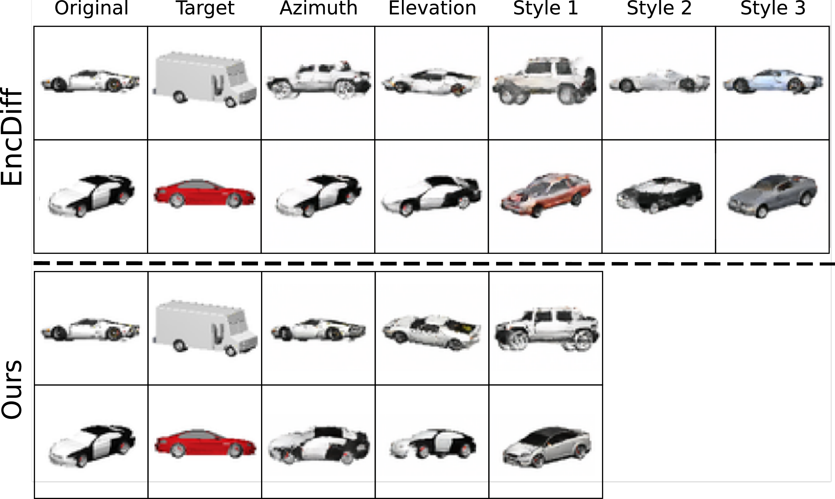
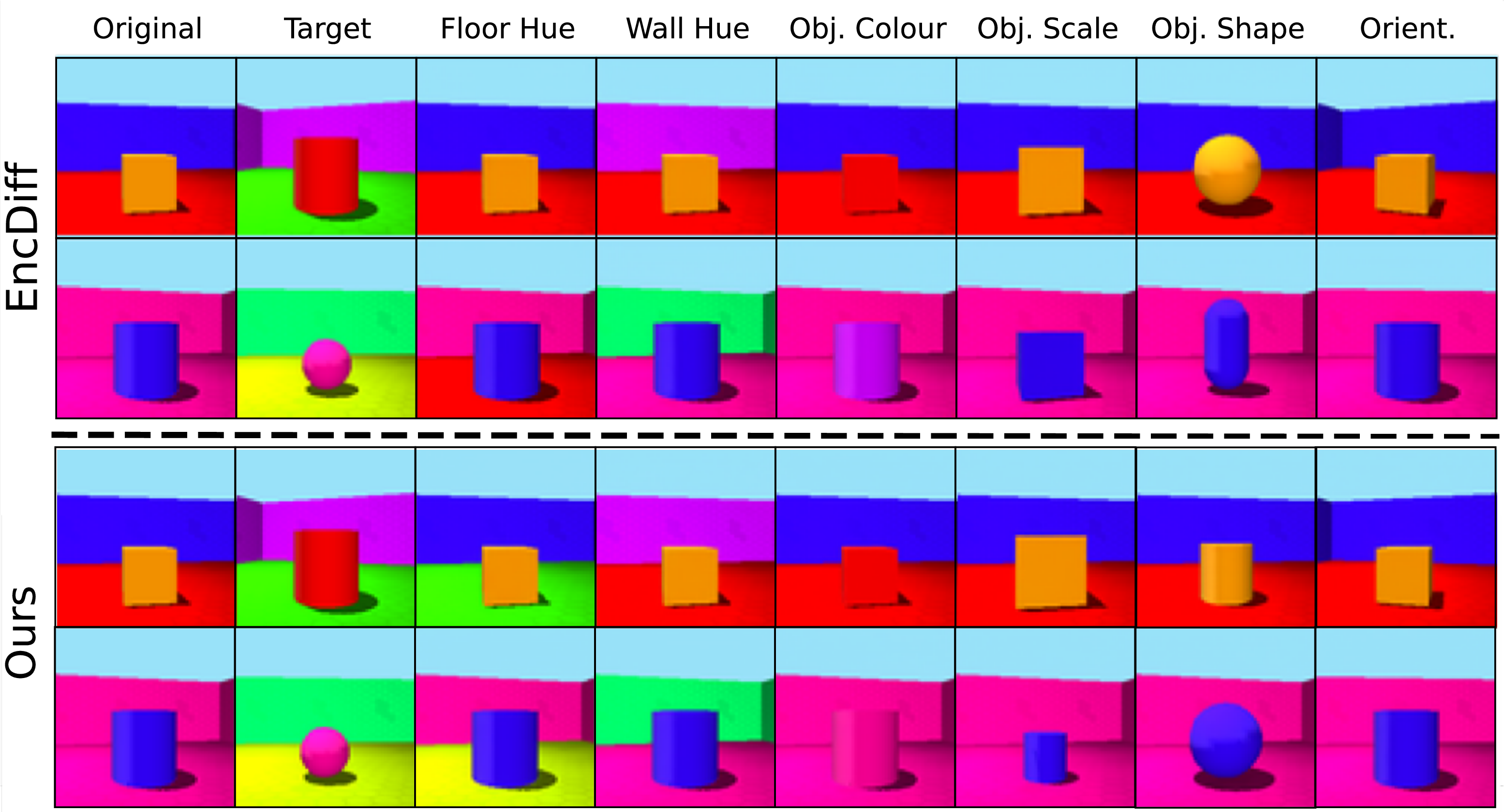
Figure 5: Latent feature discovery and controlled image editing. We manually select latent dimensions for semantic attributes in a target and transfer them to a source. On Cars3D, SteeringDRL
often isolates the challenging Style/Object Type factor in a single variable, producing more faithful edits of Azimuth and Elevation. On Shapes3D with \(N\)=10 tokens, SteeringDRL successfully performs all attribute edits, while EncDiff struggles with Floor Hue and Object Shape..
6.1 Attribute Disentanglement↩︎
We study unsupervised attribute disentanglement on Shapes3D [33], Cars3D [81], and MPI3D-Toy [82], where scalars in \(\mathbf{z}\) should capture the true generative factors of the dataset. We follow the evaluation protocol from 4, now building on top of a better parameterised U-Net taken from EncDiff [27]. We use the loss in 1 and the \(\log \mathrm{SNR}\) curriculum as defined in 3 .
Inductive Biases in SteeringDRL. In 1, we progressively apply our inductive biases to EncDiff [27] on Shapes3D. We replace the split-MLP with a parameter-efficient amortised encoder (10.1), matching the performance of vanilla EncDiff. With EncDiff, the \(\mathrm{sigmoid(-\lambda)}\) loss-weighting improves average disentanglement but increases variance; adding our curriculum does not consistently improve performance. In contrast, when combined with our gated residual U-Net, these components maintain strong performance with substantially reduced variance. 3 shows the corresponding optimisation trajectories. When using a larger U-Net than 4, the baseline no longer exhibits regime separation and instead follows the reconstruction regime. In this case, adding SteeringDRL steers trajectories toward the disentanglement regime, improving disentanglement without sacrificing reconstruction. In 4, we show that curricula can select different regimes, with the disentanglement-oriented trajectory showing better performance under the settings tested. Varying the initial band changes the optimisation trajectory, while \(m_{\max}\) determines the convergence speed within a regime. Overall, this shows that the curriculum selects the optimisation regime, while our architectural bottlenecks and loss-weighting improve stability within it (see 12.3).
Comparison to Baselines. In 2, we compare SteeringDRL from 1 to prior diffusion-based methods. For \(N = 20\), our model outperforms prior work on Cars3D and Shapes3D in both FactorVAE and DCI, and shows lower variance across seeds. For \(N = 10\), closer to the true number of generative
factors, we see larger gains over EncDiff. On MPI3D-toy, we achieve the best DCI at \(N = 20\) and remain competitive on other metrics. In 5, our improvements on Cars3D can be
attributed to better isolation of the challenging Style/Object Type factor, which EncDiff spreads over multiple latents. On Shapes3D with \(N=10\), our model recovers all ground-truth factors, while EncDiff
often confuses Floor Hue, Wall Hue, and Object Shape. Overall, our model improves disentanglement and stability, with latents better aligned to true generative factors.
6.2 Spatial Disentanglement with Object-Centric Learning↩︎
| Segmentation | Recon. | Comp. | |||
|---|---|---|---|---|---|
| 2-4 (lr)5-5 (lr)6-6 Method | FG-ARI \(\uparrow\) | mIoU \(\uparrow\) | mBO \(\uparrow\) | LPIPS \(\downarrow\) | FID \(\downarrow\) |
| SLATE [84] \(\dagger\) | \(61.39 \pm 9.07\) | \(55.00 \pm 5.47\) | \(56.40 \pm 7.19\) | \(0.397 \pm 0.009\) | \(90.26 \pm 3.72\) |
| SLATE\(^{+}\) [26] | \(70.71 \pm 3.35\) | \(52.96 \pm 1.40\) | \(54.90 \pm 1.15\) | – | \(69.23\) |
| SlotDiffusion (50 steps, DDIM) [25] \(\dagger\) | \(63.90 \pm 5.11\) | \(55.92 \pm 1.17\) | \(58.83 \pm 1.70\) | \(0.167 \pm 0.011\) | \(42.95 \pm 3.07\) |
| StableLSD (200 steps, DDPM) [26] | \(64.41 \pm 8.53\) | \(62.52 \pm 1.88\) | \(63.93 \pm 1.93\) | – | \(29.53\) |
| Modular IB [31] | \(\mathbf{87.68}\) | \(58.88\) | \(59.12\) | – | – |
| MetaSlot [85] | \(77.60 \pm 1.10\) | \(64.20 \pm 0.60\) | \(62.80 \pm 0.70\) | – | – |
| SteeringDRL (50 steps, DDIM) \(\dagger\) | \(74.39 \pm 4.12\) | \(\mathbf{68.31 \pm 2.39}\) | \(\mathbf{69.69 \pm 2.07}\) | \(0.157 \pm 0.005\) | \(26.67 \pm 2.17\) |
| SteeringDRL (200 steps, DDPM) \(\dagger\) | " | " | " | \(\mathbf{0.147 \pm 0.005}\) | \(\mathbf{23.36 \pm 2.01}\) |


Figure 6: Optimisation trajectories support visual improvements. (a) SteeringDRL discovers more objects with more complete segmentations than SlotDiffusion. (b) Compositions preserve object structure and background textures. (c) Optimisation trajectories are similar to attribute disentanglement (3), converging to higher segmentation scores than the SlotDiffusion baseline.. a — Segmentations., b — Random Compositions, c — Optimisation Trajectories.
We study spatial disentanglement with OCL on ClevrTex [83] and PascalVOC [86], using segmentation metrics on \(\mathcal{M}\) as a proxy for representation quality. We build on SlotDiffusion [25], follow its evaluation protocol, and use the objective in 2 with curriculum in 10.2. We use an effective \(\mathrm{sigmoid}(-\lambda)\) weighting, and a neutral initial band \([-2,2]\) with \(m_{\max} = 200\)k for the curriculum; ClevrTex uses \(\mathbf{x}_0\)-prediction (8.2) and PascalVOC uses \(\boldsymbol{\epsilon}\)-prediction.
Synthetic Dataset (ClevrTex). In 3, SteeringDRL outperforms prior models on mBO and mIoU, including those with additional object-centric inductive biases (ModularIB, MetaSlot). This is driven by improved segmentation of occluded objects and regions with low foreground-background contrast (6 (a)), where SlotDiffusion often under-segments or misses objects. Improved composition and reconstruction are linked to better preservation of background textures (6 (b)). Notably, 6 (c) shows that our model exhibits optimisation dynamics similar to the attribute disentanglement setting (3), while learning semantics faster and converging to higher segmentation scores than SlotDiffusion. This is consistent with H1 and H2; controlling early noise-level exposure and introducing a skip bottleneck can also steer larger models toward stronger spatial representations.
| Model | FG-ARI | mIoU\(_i\) | mIoU\(_c\) | mBO\(_i\) | mBO\(_c\) |
|---|---|---|---|---|---|
| SA + DINO ViT [11] | 12.3 | – | – | 24.6 | 24.9 |
| SLATE + DINO ViT [84] | 15.6 | – | – | 35.9 | 41.5 |
| DINOSAUR MLP [88] | 24.6 | 39.1 | 41.0 | 39.7 | 41.2 |
| DINOSAUR Trans. [88] | 23.1 | 42.0 | 47.5 | 43.2 | 47.8 |
| StableLSD [26] | 8.7 | 31.5 | 35.4 | 32.1 | 35.4 |
| SlotDiffusion [25] \(\dagger\) | 15.9 | 43.2 | 47.7 | 47.2 | 52.2 |
| SteeringDRL \(\dagger\) | 17.6 | 44.5 | 48.6 | 49.1 | 53.6 |


Figure 7: SteeringDRL accelerates object-centric binding with pretrained features. (a) SteeringDRL produces cleaner masks for dominant objects, while SlotDiffusion often undersegments. (b) With the same pretrained \(\mathrm{Feat}_{\psi}(\cdot)\), SteeringDRL reaches higher segmentation and reconstruction quality earlier in training than SlotDiffusion.. a — Segmentations., b — Optimisation Trajectories.
Training Efficiency with Pretrained Features (PascalVOC). We scale SteeringDRL to a much larger U-Net (\(\sim138\)M params), using a pretrained DINO ViT for \(\mathrm{Feat}_{\psi}(\cdot)\). In 4, we improve over the SlotDiffusion baseline on all metrics, and remain competitive with prior methods on FG-ARI. These results are competitive with baselines using higher-capacity generative models (StableLSD) and non-generative approaches (DINOSAUR). Our improvements stem from better segmentation of dominant objects that SlotDiffusion often merges (7 (a)). We also find meaningful unannotated regions. 7 (b) shows different trajectories to ClevrTex despite using a similar curriculum. On ClevrTex, where \(\mathrm{Feat}_{\psi}(\cdot)\) is learned from scratch, representations and reconstructions are learned together progressively. With pretrained features, semantics are already available, so learning shifts from feature discovery to slot binding, allowing SteeringDRL to converge faster than SlotDiffusion while reaching better segmentation and reconstruction (see 12.8.2 for more results).
7 Conclusion↩︎
We studied a key challenge in diffusion autoencoders for unsupervised disentanglement: models can attain similar reconstruction quality with substantially different representations. We trace this to early commitment to trajectories that prioritise reconstruction or semantic organisation. This motivates SteeringDRL: gated residual U-Nets targeting shortcut pathways (H1) and a \(\log \mathrm{SNR}\) curriculum controlling early noise-level exposure (H2). Although regime separation is clearest in low-capacity settings, these mechanisms lead to effective interventions in larger models. SteeringDRL changes optimisation dynamics to improve attribute and spatial disentanglement across datasets. These results support H1 and H2 as design principles: restrict reconstruction shortcuts and control when models see specific noise levels. Future work should study \(\log \mathrm{SNR}\) curricula more systematically to better understand the reconstruction-representation trade-off. Different configurations change behaviour across architectures, capacities, and datasets. This is especially relevant in transformer architectures [50], [52], [75], where shortcut pathways are constrained and curriculum-based control may apply naturally. The VQ-VAE is another important inductive bias to study further (12.5).
We thank Pavithra Manoj, Fabio De Sousa Ribeiro, Xiaodan Xing, Vishal Jain, and Raghav Mehta for their detailed and insightful feedback on early versions of this manuscript. We also thank Nairouz Shehata for her support with the tooling used to produce the figures. Finally, we thank Bernhard Kainz for his support and encouragement during this project.
R.R. is supported by EPSRC through a Doctoral Training Partnerships PhD Scholarship. A.K. is supported by the EPSRC Doctoral Prize. T.X. is supported through the Imperial College London UKRI Impact Acceleration Account EP/X52556X/1. B.G. was supported by the Royal Academy of Engineering as part of the Kheiron/RAEng Research Chair.
8 Background↩︎
8.1 Cosine Noise Schedule↩︎
We use the cosine noise schedule in all of our experiments. It is defined as \[\lambda = f_\lambda(t) = -2 \log\bigg(\tan\bigg(\frac{\pi t}{2}\bigg)\bigg), \qquad t = f_\lambda^{-1}(\lambda) = \frac{2}{\pi} \arctan(e^{-\lambda/2}),\] with corresponding density \[p(\lambda) = -\frac{d}{d\lambda} f^{-1}_\lambda(\lambda) = \frac{\mathrm{sech}(\lambda / 2)}{2\pi}.\]
8.2 Objective for \(\mathbf{x}_0\)-Prediction↩︎
Our main objective is written in \(\boldsymbol{\epsilon}\)-prediction form, where the loss is weighted by \(w_{\boldsymbol{\epsilon}}(\lambda)\). For some experiments, however, we use \(\mathbf{x}_0\)-prediction. Here, we derive the equivalent weighting required for \(\mathbf{x}_0\)-prediction to induce the same effective \(\boldsymbol{\epsilon}\)-prediction objective. For variance-preserving diffusion, the forward process is \[\mathbf{x}_\lambda = \alpha_\lambda \mathbf{x}+ \sigma_\lambda \boldsymbol{\epsilon}, \qquad \alpha_\lambda^2 = \mathrm{sigmoid}(\lambda), \qquad \sigma_\lambda^2 = \mathrm{sigmoid}(-\lambda),\] so that \[\frac{\alpha_\lambda^2}{\sigma_\lambda^2} = \exp(\lambda).\] Given an \(\mathbf{x}_0\)-prediction model \(\hat{\mathbf{x}}_\theta(\mathbf{x}_\lambda;\lambda,\mathbf{S})\), the corresponding noise prediction is \[\hat{\boldsymbol{\epsilon}}_\theta(\mathbf{x}_\lambda;\lambda,\mathbf{S}) = \frac{\mathbf{x}_\lambda - \alpha_\lambda \hat{\mathbf{x}}_\theta(\mathbf{x}_\lambda;\lambda,\mathbf{S})}{\sigma_\lambda}.\] Substituting \(\mathbf{x}_\lambda = \alpha_\lambda \mathbf{x}+ \sigma_\lambda \boldsymbol{\epsilon}\) gives \[\boldsymbol{\epsilon}- \hat{\boldsymbol{\epsilon}}_\theta = \frac{\alpha_\lambda}{\sigma_\lambda} \left( \mathbf{x}- \hat{\mathbf{x}}_\theta \right).\] Therefore, \[\big\|\boldsymbol{\epsilon}- \hat{\boldsymbol{\epsilon}}_\theta\big\|_2^2 = \frac{\alpha_\lambda^2}{\sigma_\lambda^2} \big\|\mathbf{x}- \hat{\mathbf{x}}_\theta\big\|_2^2 = \exp(\lambda) \big\|\mathbf{x}- \hat{\mathbf{x}}_\theta\big\|_2^2. \label{eq:xpred95eps95equiv}\tag{4}\]
It follows that an \(\boldsymbol{\epsilon}\)-prediction objective with weighting \(w_{\boldsymbol{\epsilon}}(\lambda)\), \[w_{\boldsymbol{\epsilon}}(\lambda) \big\|\boldsymbol{\epsilon}- \hat{\boldsymbol{\epsilon}}_\theta\big\|_2^2,\] is equivalent to an \(\mathbf{x}_0\)-prediction objective with weighting \[w_\mathbf{x}(\lambda) = \exp(\lambda) w_{\boldsymbol{\epsilon}}(\lambda). \label{eq:xpred95weight95conversion}\tag{5}\] In our main experiments for attribute disentanglement, we use \[w_{\boldsymbol{\epsilon}}(\lambda) = \mathrm{sigmoid}(-\lambda).\] Using 5 , the corresponding \(\mathbf{x}_0\)-prediction weighting is \[w_\mathbf{x}(\lambda) = \exp(\lambda) \; \mathrm{sigmoid}(-\lambda) = \mathrm{sigmoid}(\lambda).\] Thus, when training \(\mathbf{x}_0\)-prediction models for spatial disentanglement with ClevrTex, we use \(w_\mathbf{x}(\lambda)=\mathrm{sigmoid}(\lambda)\) to preserve the same effective \(\boldsymbol{\epsilon}\)-space weighting as \(w_{\boldsymbol{\epsilon}}(\lambda)=\mathrm{sigmoid}(-\lambda)\).
9 Metrics↩︎
9.1 Attribute Disentanglement↩︎
For attribute disentanglement metrics (DCI, FactorVAE and MIG), we use code from [70].
DCI Disentanglement [71]. We report the disentanglement component of the DCI framework [71]. This measures whether the predictive information in each latent dimension is concentrated on a single ground-truth factor. We train a gradient-boosted tree classifier from Scikit-Learn [89] to predict each of the \(M\) ground-truth factors from the learned representation vector \(\mathbf{z} \in \mathbb{R}^D\) produced by \(\mathrm{Feat}_{\psi}(\cdot)\), using \(10{,}000\) training and \(5{,}000\) test images. We use the absolute values of the weights to form a feature importance matrix \(\mathbf{R} \in \mathbb{R}^{D \times M}\), where the rows correspond to latents and the columns to ground truth factors. For each latent dimension \(i\), we form a distribution over true factors, \[p_{ij} = \frac{R_{ij}}{\sum_{j'=1}^{M} R_{ij'}}, \qquad \mathbf{p}_i = (p_{i1}, ..., p_{iM}).\] The per-latent disentanglement score is then defined as \[D_i = 1 - H_M(\mathbf{p}_i), \qquad H_M(\mathbf{p}_i) = -\sum_{j=1}^{M} p_{ij}\log_M p_{ij}.\] If latent dimension \(i\) is important for only one ground-truth factor, then \(H_M(\mathbf{p}_i)=0\) and \(D_i=1\). If it is equally important for all \(M\) factors, then \(H_M(\mathbf{p}_i)=1\) and \(D_i=0\). The per-latent relative importance is defined by normalising each row w.r.t every cell in \(\mathbf{R}\), \[\rho_i = \frac{\sum_{j=1}^{M} R_{ij}}{\sum_{i'=1}^{D}\sum_{j=1}^{M} R_{i'j}} .\] The final score is the importance-weighted average over latent dimensions, \[\mathrm{DCI\text{-}D} = \sum_{i=1}^{D} \rho_i D_i .\] High values indicate that individual latent dimensions are predictive of single ground-truth factors. We report this value on the test samples.
FactorVAE [33]. This tests whether a fixed generative factor can be identified by finding which latent dimension changes the least. We first estimate the global variance of each latent coordinate in \(\mathbf{z} \in \mathbb{R}^D\) using \(10{,}000\) training images, and prune inactive dimensions whose standard deviation is below \(0.05\). Then, we repeatedly sample mini-batches of size \(64\), with the value of one ground-truth factor \(v_j\) fixed across the batch, and sampling all other factors randomly. For each mini-batch, we compute the variance of each active latent coordinate and normalise it by its global variance. The active latent dimension with the smallest normalised variance casts a vote for the fixed factor \(v_j\). Aggregating these votes over \(10{,}000\) images gives a majority-vote classifier from latent dimensions to factors. We report the accuracy of this classifier on \(5{,}000\) test samples. High values indicate that fixing a ground-truth factor reliably makes one latent dimension remain stable while the others vary.
Mutual Information Gap (MIG) [34]. This measures whether each ground-truth factor is captured by one clearly dominant latent dimension rather than being spread across several latents. We sample \(10{,}000\) images and compute their learned representations \(\mathbf{z} \in \mathbb{R}^D\). Each latent dimension \(z_i\) is discretised into \(20\) bins, after which we estimate the discrete mutual information between every discretised latent dimension \(\widetilde{z}_i \in \{1, ..., 20\}\) and every ground-truth factor \(v_j\). This gives a mutual information matrix \(\mathbf{M} \in \mathbb{R}^{D \times M}\), where \(M_{ij} = I(\widetilde{z}_i, v_j)\). For each factor \(v_j\), we sort the mutual information values across latent dimensions and compute the gap between the largest and second-largest values, normalised by the entropy \(H(v_j)\): \[\mathrm{MIG} = \frac{1}{M} \sum_{j=1}^{M} \frac{ M_{(1)j} - M_{(2)j} }{ H(v_j) },\] where \(M_{(1)j}\) and \(M_{(2)j}\) denote the largest and second-largest entries in column \(j\) of \(\mathbf{M}\). High values indicate that each ground-truth factor has a single dominant latent dimension that contains substantially more information about it than any other latent dimension.
9.2 Spatial Disentanglement↩︎
For the segmentation metrics for spatial disentanglement (FG-ARI, mBO, mIoU), we use the code from [25]. All of these metrics are converted to percentages for our tables.
Foreground Adjusted Rand Index (FG-ARI) [90], [91], rand1971objective?. This measures whether foreground pixels that belong to the same ground-truth object are assigned to the same predicted segment. The adjusted Rand Index (ARI) measures clustering similarity between pixels in a ground truth and predicted mask, where a score of \(1\) corresponds to perfect agreement, while a score near \(0\) corresponds to chance-level agreement. Following common practice in object-centric learning [13], we exclude pixels labelled as background in the ground-truth mask before computing ARI. Higher values indicate that foreground object instances are better recovered. Since FG-ARI ignores ground-truth background pixels, it does not penalise errors that only affect background segmentation [83], [92].
Mean Intersection-over-Union (mIoU). This measures the spatial overlap between predicted masks and ground-truth masks. For a predicted mask \(P\) and ground-truth mask \(G\), the IoU is \[\mathrm{IoU}(P,G) = \frac{|P \cap G|}{|P \cup G|}.\] Since predicted slots are unordered, we first compute all pairwise IoUs between predicted masks and the relevant ground-truth masks, and then use Hungarian matching to find an assignment that maximises total IoU. The matched IoUs are averaged to obtain mIoU. We report both instance-wise and class-wise variants. For \(\mathrm{mIoU}_i\), the ground-truth masks correspond to object instances. For \(\mathrm{mIoU}_c\), the ground-truth masks correspond to semantic classes. Thus, \(\mathrm{mIoU}_i\) measures recovery of individual object instances, while \(\mathrm{mIoU}_c\) measures semantic class-level overlap. Higher values indicate better spatial agreement between predicted and ground-truth masks.
Mean Best Overlap (mBO). Mean best overlap also measures mask overlap, but unlike mIoU it does not enforce a one-to-one matching between predicted and ground-truth masks. For each ground-truth mask \(G_k\), we compute its best overlap with any predicted mask, \[\mathrm{BO}(G_k) = \max_l \frac{|G_k \cap P_l|}{|G_k \cup P_l|},\] where \(\{P_l\}\) are the predicted masks. The mean best overlap is then \[\mathrm{mBO} = \frac{1}{K} \sum_{k=1}^{K} \mathrm{BO}(G_k).\] We report both instance-wise and class-wise variants. For \(\mathrm{mBO}_i\), the ground-truth masks \(\{G_k\}_{k=1}^{K}\) correspond to object instances. For \(\mathrm{mBO}_c\), they correspond to semantic classes. Thus, \(\mathrm{mBO}_i\) measures whether each object instance is covered by at least one predicted mask, while \(\mathrm{mBO}_c\) measures whether each semantic class region is covered by at least one predicted mask. Higher values indicate better best-case overlap between ground-truth masks and predicted masks.
10 Method↩︎
10.1 Amortised Semantic Encoder with FiLM Modulation↩︎
To improve the parameter efficiency of the semantic encoder (3.2), we design \(\mathrm{IB}_{\kappa}(\cdot)\) attribute disentanglement using a shared backbone with FiLM modulation [76] in place of the split-MLP [27], \[\boldsymbol{Split-MLP:} \quad \mathbf{s}_i = \mathrm{IB}_{\xi_i}(z_i), \qquad \boldsymbol{Ours:} \quad \mathbf{s}_i = \mathrm{IB}_{\xi}\big(z_i; \{ \gamma_i^{(l)}, \beta_i^{(l)} \}_{l=1}^{L}\big),\] where the split-MLP uses separate parameters \(\xi_i\) for each latent scalar \(z_i\), while our approach shares weights \(\xi\) across all latents. The FiLM parameters \(\{\gamma_i^{(l)}, \beta_i^{(l)}\}_{l=1}^{L}\) provide latent-specific feature-wise modulation across \(L\) layers of the shared network via scaling and shifting of intermediate activations. This design preserves factor-wise independence (each token \(\mathbf{s}_i\) depends only on the scalar \(z_i\)) while reducing parameters by approximately \(\mathcal{O}(N)\). In this work, we set \(L = 2\). We found this to provide similar disentanglement as the split-MLP, seen in 1, when paired with a deeper feature extractor, which we refer to as Residual ConvNet in 5.
10.2 Deriving the \(\log \mathrm{SNR}\) Curriculum Loss↩︎
Our curriculum restricts training at step \(m\) to an active \(\log \mathrm{SNR}\) band \([\lambda_L(m), \lambda_U(m)]\). This defines the truncated density \[q(\lambda;m) = \frac{p(\lambda)}{Z(m)} \mathbf{1}\{\lambda \in [\lambda_L(m), \lambda_U(m)]\}, \qquad Z(m) = \int_{\lambda_L(m)}^{\lambda_U(m)} p(\lambda)\,d\lambda .\] Sampling from \(q(\lambda;m)\) therefore requires the importance correction \[\frac{w(\lambda)}{q(\lambda;m)} = Z(m)\frac{w(\lambda)}{p(\lambda)} .\] Thus, the curriculum objective in \(\lambda\)-space is \[\mathcal{L}(\mathbf{x},\mathbf{S};m) = \frac{1}{2} \mathbb{E}_{\boldsymbol{\epsilon}\sim\mathcal{N}(0,\mathbf{I}),\,\lambda\sim q(\lambda;m)} \left[ Z(m)\frac{w(\lambda)}{p(\lambda)} \big\| \boldsymbol{\epsilon}-\hat{\boldsymbol{\epsilon}}_\theta(\mathbf{x}_\lambda;\lambda,\mathbf{S}) \big\|_2^2 \right]. \label{eq:curriculum95importance95appendix}\tag{6}\]
Equivalently, when implementing the objective by sampling time, we sample \(t\) uniformly over the corresponding active time interval \([t_U(m), t_L(m)]\), where \(t_U(m)=f_\lambda^{-1}(\lambda_U(m))\) and \(t_L(m)=f_\lambda^{-1}(\lambda_L(m))\). For decreasing noise schedules, this interval has mass \[Z(m) = t_L(m)-t_U(m).\] Using \(\lambda=f_\lambda(t)\), the derivative-form curriculum objective is then \[\mathcal{L}(\mathbf{x},\mathbf{S};m) = \frac{1}{2} \mathbb{E}_{\boldsymbol{\epsilon}\sim\mathcal{N}(0,\mathbf{I}),\,t\sim\mathcal{U}(t_U(m),t_L(m))} \left[ Z(m)\, w(\lambda) \left(-\frac{d\lambda}{dt}\right) \big\| \boldsymbol{\epsilon}-\hat{\boldsymbol{\epsilon}}_\theta(\mathbf{x}_\lambda;\lambda,\mathbf{S}) \big\|_2^2 \right]. \label{eq:curriculum95deriv95appendix}\tag{7}\]
11 Experimental Setup↩︎
11.1 Analysis↩︎
For the trajectory analysis in 4, we modify the lightweight imagev3 U-Net implementation from k-diffusion1 by
adding EncDiff SpatialTransformer blocks for conditioning on the output of \(\mathrm{Enc}_\phi(\cdot)\), together with a middle bottleneck layer. This U-Net uses fixed convolutions for up- and down-sampling. We use the
Encoder4 encoder for \(\mathrm{Feat}_{\psi}(\cdot)\) and the split-MLP for \(\mathrm{IB}_{\kappa}(\cdot)\) from EncDiff [27] to construct \(\mathrm{Enc}_\phi(\cdot)\). Models are trained until they have seen 3M images, which is sufficient for most runs to reach stable
reconstruction and disentanglement scores. For this analysis, we use the EncDiff VQ-VAE checkpoint trained for 30K steps. We use 5 model initialisation seeds and 5 \(\lambda\)-sampling seeds, giving 25 runs in total. This
lets us test whether early disentanglement correlates with model initialisation or noise-level sampling; we did not find strong evidence for either. As discussed in 12.5, this checkpoint makes regime
separation more visible, whereas longer VQ-VAE training improves reconstruction and reduces the separation between regimes.
11.2 Main Experiments↩︎
Architecture and training details for all datasets are summarised in 5.
For the main attribute disentanglement experiments, we follow EncDiff [27] unless otherwise specified. We use the same datasets, evaluation protocol, and VQ-VAE architecture, while replacing the split-MLP encoder with our Scalar-to-Token FiLM encoder and the standard U-Net with our gated residual U-Net. All attribute models use \(\boldsymbol{\epsilon}\)-prediction with \(\mathrm{sigmoid}(-\lambda)\) weighting and the \(\log \mathrm{SNR}\) curriculum described in 5.2. We train until the model has seen 15M images, which is sufficient for convergence. This takes approximately 16 hours on an NVIDIA A40 or 10 hours on an NVIDIA RTX 4090.
For object-centric learning, we build on SlotDiffusion [25], instantiate \(\mathrm{IB}_{\kappa}(\cdot)\) with Slot Attention, and follow its evaluation protocol on ClevrTex and PascalVOC. ClevrTex uses \(\mathbf{x}_0\)-prediction with the equivalent weighting in 8.2, while PascalVOC uses \(\boldsymbol{\epsilon}\)-prediction. We use the VQ-VAE checkpoints provided by the SlotDiffusion codebase. For fair comparison to SlotDiffusion, we train ClevrTex for 400 epochs and PascalVOC for 500 epochs. Trajectory plots are computed on the validation set for ClevrTex. For PascalVOC, the val and test set are the same in the SlotDiffusion evaluation protocol. On H100 GPUs, both object-centric models can be trained within one day.
| Dataset | Shapes3D | Cars3D | MPI3D | ClevrTex | PascalVOC |
|---|---|---|---|---|---|
| Feature Extractor (\(\Feat(\cdot)\)) | Residual ConvNet | Residual ConvNet | Residual ConvNet | ResNet34 | DINO ViT-S/8 |
| Disentanglement Inductive Bias (\(\IB(\cdot)\)) | Amortised FiLM | Amortised FiLM | Amortised FiLM | Slot Attention | Slot Attention |
| Number of Tokens / Slots (\(N\)) | 10/20 | 10/20 | 10/20 | 11 | 6 |
| Token / Slot Dimension | 16 | 16 | 16 | 192 | 192 |
| Slot Attention Iterations | – | – | – | 3 | 3 |
| Prediction Target | \(\veps\) | \(\veps\) | \(\veps\) | \(\x_0\) | \(\veps\) |
| Loss Weighting | \(\mathrm{Sigmoid}(-\lambda)\) | \(\mathrm{Sigmoid}(-\lambda)\) | \(\mathrm{Sigmoid}(-\lambda)\) | \(\mathrm{Sigmoid}(\lambda)\) | \(\mathrm{Sigmoid}(-\lambda)\) |
| Initial Curriculum Band (\([\lambda_L(0), \lambda_U(0)]\)) | \([0, 10]\) | \([0, 10]\) | \([0, 10]\) | \([-2,2]\) | \([-2,2]\) |
| Full \(\logsnr\) Band (\([\lambda_{\min}, \lambda_{\max}]\)) | \([-5,12]\) | \([-5,12]\) | \([-5,12]\) | \([-8.5, 6.5]\) | \([-15, 15]\) |
| Widening Steps (\(m_{\max}\)) | \(32\)K | \(32\)K | \(32\)K | \(200\)K | \(200\)K |
| Learning Rate | \(5{\times}10^{-4}\) | \(5{\times}10^{-4}\) | \(5{\times}10^{-4}\) | \(10^{-4}\) | \(10^{-4}\) |
| LR Schedule | Constant | Constant | Constant | Cosine | Cosine |
| EMA | U-Net + encoder EMA; inverse warmup, max \(0.9999\) | – | – | ||
| Optimiser | AdamW | AdamW | AdamW | Adam | Adam |
| Batch Size | 128 | 128 | 128 | 64 | 64 |
| Base U-Net Architecture | EncDiff [27] | SlotDiffusion [25] | |||
| Base VQ-VAE Architecture | [63] with LPIPS Discriminator | Ckpts from SlotDiffusion Repo [25] | |||
| Latent Resolution \(\x_{0}\) | \(16{\times}16\) | \(16{\times}16\) | \(16{\times}16\) | \(32{\times}32\) | \(56{\times}56\) |
11.3 OCL Curricula↩︎
This is the curriculum we use for the PascalVOC dataset (6.2). It is more neutral than the curriculum used for ClevrTex (2 (b)), which steers towards the disentanglement regime.
12 Additional Results↩︎
12.1 Optimisation Trajectories↩︎
We repeat the trajectory analysis from 1 under alternative loss-weighting functions. In [fig:shapes3d95regimes95sech], we use the non-monotonic weighting \(w(\lambda)=\mathrm{sech}(\lambda)\), which places most weight near intermediate \(\log \mathrm{SNR}\) values, akin to the EDM with shift \(-3\) we used in 4. The same qualitative behaviour appears; runs separate into trajectories that prioritise reconstruction early and trajectories that maintain stronger disentanglement throughout training. This suggests that the regime structure is not specific to a single loss-weighting choice, but reflects a broader optimisation property of diffusion autoencoders in this low-capacity setting.
12.2 Cross-Attention Maps in each Regime↩︎
We visualise cross-attention maps from the low-capacity U-Net used in 4. We use the second downsampling layer in the U-Net encoder, which operates at spatial resolution \(8^2\), and visualise maps at the same layer and logSNR level for both models. For readability, attention maps are upsampled and smoothed. [fig:shapes3d95regimes95cross95attn] compares models from the reconstruction and disentanglement regimes. Although both models achieve strong reconstructions, their internal attention patterns differ substantially. In the disentanglement regime, several attention maps are spatially localised and align with all ground-truth factors. In contrast, attention maps in the reconstruction regime are more diffuse and less consistently aligned with individual factors. This supports the interpretation that the two regimes correspond not only to different metric values, but also to different internal representations.
12.3 Skip Connections↩︎
| Model | LPIPS \(\downarrow\) | DCI \(\uparrow\) | FactorVAE \(\uparrow\) | MIG \(\uparrow\) |
|---|---|---|---|---|
| EncDiff U-Net + Split-MLP [27] | \(0.0025 \pm 0.0003\) | \(0.828 \pm 0.099\) | \(0.921 \pm 0.093\) | \(0.218 \pm 0.087\) |
| + \(\mathrm{sigmoid(-\lambda)}\)* | \(\mathbf{0.0020 \pm 0.0001}\) | \(0.932 \pm 0.077\) | \(0.971 \pm 0.056\) | \(0.399 \pm 0.102\) |
| + \(\logsnr\) Curriculum | \(0.0020 \pm 0.0003\) | \(0.853 \pm 0.060\) | \(0.917 \pm 0.063\) | \(0.299 \pm 0.066\) |
| Zeroed Skips + \(\mathrm{sigmoid(-\lambda)}\)* | \(0.1573 \pm 0.0221\) | \(0.905 \pm 0.079\) | \(0.940 \pm 0.062\) | \(0.439 \pm 0.109\) |
| + \(\logsnr\) Curriculum | \(0.2029 \pm 0.0049\) | \(\mathbf{0.942 \pm 0.064}\) | \(\mathbf{0.975 \pm 0.059}\) | \(\mathbf{0.548 \pm 0.161}\) |
| Skip Dropout [66] + \(\mathrm{sigmoid(-\lambda)}\) | \(0.0030 \pm 0.0003\) | \(0.892 \pm 0.075\) | \(0.954 \pm 0.052\) | \(0.408 \pm 0.088\) |
| + \(\logsnr\) Curriculum | \(0.0030 \pm 0.0002\) | \(0.876 \pm 0.101\) | \(0.935 \pm 0.061\) | \(0.397 \pm 0.123\) |


Figure 8: Removing skip connections steers trajectories toward disentanglement. We follow the setup in Figure 1 and compare the EncDiff baseline against zeroed-skip variants. Zeroing skip connections shifts optimisation trajectories upward toward the disentanglement regime, but also moves them leftward more slowly, reflecting worse reconstruction. Adding the \(\log \mathrm{SNR}\) curriculum on top of zeroed skips steers trajectories to the high-disentanglement region, especially for MIG. Together with Table 6, these results support H1: skip connections act as reconstruction-oriented shortcuts, and regulating them can make optimisation rely more on the representation pathway.. a — Zeroed skips., b — Zeroed skips + \(\log \mathrm{SNR}\) curriculum from \([0, 10]\) to \([-5, 12]\) over \(32\)K steps.
We test the role of skip connections in unsupervised diffusion representation learning by modifying the skip pathways of the EncDiff U-Net used in our Shapes3D analysis. In the zeroed skips setting, we replace the encoder skip features passed to the decoder with zeros, removing the shortcut pathway and forcing the decoder to rely more heavily on the U-Net trunk and conditioning representation. We also compare against Skip Dropout [66], which stochastically drops skip-connection features.
6 shows that removing skip information strongly improves disentanglement, but at a substantial cost to reconstruction. Zeroing skips improves DCI, FactorVAE and MIG relative to the EncDiff U-Net, and the \(\log \mathrm{SNR}\) curriculum further increases disentanglement. However, reconstruction degrades sharply, indicating that the skip pathway is useful for image fidelity even when it is harmful for representation learning. Skip Dropout gives a softer version of this effect, preserving reconstruction quality while improving disentanglement, but the gains are smaller and the \(\log \mathrm{SNR}\) curriculum does not further improve performance. This mirrors the behaviour of the standard U-Net with curriculum in 1, suggesting that when skip connections are present, their reconstruction bias can dominate the curriculum signal.
The trajectory plots in 8 make this behaviour visible. With zeroed skips, trajectories shift toward the disentanglement regime, achieving higher final representation scores but worse LPIPS. Adding the \(\log \mathrm{SNR}\) curriculum preserves this shift and further concentrates trajectories in the high-disentanglement region, particularly for MIG. Together, these results support H1: skip connections are not merely an implementation detail, but a reconstruction-oriented shortcut that can determine whether optimisation uses the representation pathway or bypasses it.
Zeroed skips + \(\log \mathrm{SNR}\) curriculum. The zeroed-skips + \(\log \mathrm{SNR}\) curriculum ablation directly probes the interaction between H1 and H2. Removing skip pathways shifts trajectories toward the disentanglement regime, while adding the \(\log \mathrm{SNR}\) curriculum shifts them further into the disentanglement region, especially for MIG. This suggests that noise-level exposure can steer optimisation more effectively once reconstruction shortcuts are restricted. Together, this supports our main conclusion: the curriculum selects the optimisation regime, while architectural bottlenecks and loss-weighting improve stability within it. Since zeroing skips sharply degrades reconstruction, we instead regulate skip pathways with gated residuals, preserving a weaker reconstruction pathway.
12.4 Early Noise-Level Exposure↩︎
7 shows an early-time slice at \(320\)K images, using the 150K VQ-VAE checkpoint. The three bands are chosen to distinguish full noise-level support, removal of high-noise levels, and high-noise only. The full band \([-5,12]\) gives the strongest early reconstruction among the three settings, reaching LPIPS \(0.0348 \pm 0.0138\), while also achieving competitive disentanglement. Removing high-noise levels with \([0,12]\) slows reconstruction, increasing LPIPS to \(0.1721 \pm 0.0413\), but does not collapse the representation: DCI and FactorVAE decrease moderately, while MIG remains comparable to the full band. Conversely, the high-noise band \([-5,0]\) gives the worst reconstruction, with LPIPS \(0.2929 \pm 0.0021\), but the strongest early disentanglement scores. These results show that early noise-level exposure changes the relative pace of reconstruction and semantic organisation: full support accelerates reconstruction, whereas restricted bands preserve or improve early disentanglement despite worse image fidelity. This supports H2: noise-level exposure changes the path through reconstruction-disentanglement space, and may therefore influence regime selection.
| Description | \(\lambda_{\min}\) | \(\lambda_{\max}\) | LPIPS\(\downarrow\) | DCI\(\uparrow\) | FactorVAE\(\uparrow\) | MIG\(\uparrow\) |
|---|---|---|---|---|---|---|
| Full band | \(-5\) | \(12\) | \(0.0348 \pm 0.0138\) | \(0.614 \pm 0.053\) | \(0.716 \pm 0.122\) | \(0.100 \pm 0.049\) |
| No high-noise | \(0\) | \(12\) | \(0.1721 \pm 0.0413\) | \(0.508 \pm 0.073\) | \(0.673 \pm 0.078\) | \(0.118 \pm 0.073\) |
| Only high-noise | \(-5\) | \(0\) | \(0.2929 \pm 0.0021\) | \(0.635 \pm 0.070\) | \(0.786 \pm 0.065\) | \(0.184 \pm 0.063\) |
12.5 Noise-Level Exposure and Latent Autoencoder Effects↩︎
To isolate the role of noise-level support, we train the toy diffusion autoencoder with fixed \(\log \mathrm{SNR}\) bands under the \(\mathrm{sigmoid}(-\lambda)\) loss-weighting used in our main experiments. We report results with two VQ-VAE checkpoints: an earlier 30K-step checkpoint used for the trajectory analysis in 4, and a later 150K-step checkpoint used to more closely follow EncDiff and obtain stronger reconstruction. The 30K VQ-VAE produces the clearest optimisation regimes, while the 150K VQ-VAE improves reconstruction and makes the regime separation less pronounced.
The fixed-band ablations show that reconstruction is highly sensitive to the high-noise part of the objective, whereas disentanglement is less tied to full noise-level support. For the 30K VQ-VAE, removing high-noise levels worsens LPIPS from \(0.0177\) to \(0.4044\), but disentanglement does not collapse: FactorVAE and MIG increase, while DCI decreases. The strongest disentanglement for this checkpoint comes from restricted bands, with \([-5,5]\) giving the best DCI and FactorVAE, and \([0,12]\) giving the best MIG. However, using only high-noise levels \([-5,0]\) performs poorly across all disentanglement metrics, suggesting that high-noise exposure alone is insufficient to organise factors in \(\mathbf{z}\). For the 150K VQ-VAE, removing high-noise levels again worsens reconstruction, increasing LPIPS from \(0.0017\) to \(0.0671\), and using only high-noise levels gives very poor LPIPS (\(0.2975\)). Disentanglement varies less sharply for this later checkpoint, but restricted bands remain competitive with the full band, with several bands improving FactorVAE or MIG despite worse reconstruction. Thus, full-band training is best for reconstruction, but not uniquely best for disentanglement.
| Description | \(\lambda_{\min}\) | \(\lambda_{\max}\) | LPIPS \(\downarrow\) | DCI \(\uparrow\) | FactorVAE \(\uparrow\) | MIG \(\uparrow\) |
|---|---|---|---|---|---|---|
| Full band | \(-5\) | \(12\) | \(0.0017 \pm 0.0007\) | \(0.744 \pm 0.093\) | \(0.814 \pm 0.085\) | \(0.186 \pm 0.085\) |
| No high-noise | \(0\) | \(12\) | \(0.0671 \pm 0.0167\) | \(0.703 \pm 0.117\) | \(0.793 \pm 0.120\) | \(0.231 \pm 0.123\) |
| No low-noise | \(-5\) | \(10\) | \(0.0015 \pm 0.0002\) | \(0.684 \pm 0.041\) | \(0.789 \pm 0.045\) | \(0.176 \pm 0.045\) |
| No extremes | \(0\) | \(10\) | \(0.0614 \pm 0.0182\) | \(0.716 \pm 0.071\) | \(0.825 \pm 0.082\) | \(0.231 \pm 0.109\) |
| Middle band | \(-5\) | \(5\) | \(0.0021 \pm 0.0001\) | \(0.722 \pm 0.064\) | \(0.829 \pm 0.107\) | \(0.187 \pm 0.069\) |
| Only high-noise | \(-5\) | \(0\) | \(0.2975 \pm 0.0006\) | \(0.739 \pm 0.097\) | \(0.859 \pm 0.096\) | \(0.231 \pm 0.071\) |
| Description | \(\lambda_{\min}\) | \(\lambda_{\max}\) | LPIPS \(\downarrow\) | DCI \(\uparrow\) | FactorVAE \(\uparrow\) | MIG \(\uparrow\) |
|---|---|---|---|---|---|---|
| Full band* | \(-5\) | \(12\) | \(0.0177 \pm 0.0399\) | \(0.750 \pm 0.102\) | \(0.868 \pm 0.088\) | \(0.268 \pm 0.121\) |
| No high-noise* | \(0\) | \(12\) | \(0.4044 \pm 0.0725\) | \(0.665 \pm 0.202\) | \(0.892 \pm 0.153\) | \(0.381 \pm 0.157\) |
| No low-noise | \(-5\) | \(10\) | \(0.0054 \pm 0.0012\) | \(0.790 \pm 0.105\) | \(0.872 \pm 0.122\) | \(0.283 \pm 0.139\) |
| No extremes | \(0\) | \(10\) | \(0.3938 \pm 0.0892\) | \(0.694 \pm 0.158\) | \(0.917 \pm 0.112\) | \(0.358 \pm 0.147\) |
| Middle band | \(-5\) | \(5\) | \(0.0063 \pm 0.0011\) | \(0.834 \pm 0.118\) | \(0.926 \pm 0.085\) | \(0.313 \pm 0.134\) |
| Only high-noise | \(-5\) | \(0\) | \(0.2021 \pm 0.0006\) | \(0.641 \pm 0.069\) | \(0.778 \pm 0.083\) | \(0.166 \pm 0.059\) |
These results motivate our curriculum. Rather than removing reconstruction-favouring noise levels entirely, we delay exposure to them. This gives the representation time to organise under a bounded noise range before the model sees the full reconstruction objective. The VQ-VAE checkpoint also matters: as the VQ-VAE is trained longer, reconstruction improves, but disentanglement becomes less separated across bands. One possible explanation is that a more mature VQ-VAE encodes finer visual detail directly in the latent space, making reconstruction easier and reducing the pressure to organise information through \(\mathbf{z}\). We therefore use the 30K VQ-VAE to study regime emergence, where the effect is most visible, and the 150K VQ-VAE for experiments that more closely follow EncDiff.
| Description | \(\lambda_{\min}\) | \(\lambda_{\max}\) | \(\Delta\) LPIPS \(\downarrow\) | \(\Delta\) DCI \(\uparrow\) | \(\Delta\) FactorVAE \(\uparrow\) | \(\Delta\) MIG \(\uparrow\) |
|---|---|---|---|---|---|---|
| Full band | \(-5\) | \(12\) | \(-0.904\) | \(-0.008\) | \(-0.062\) | \(-0.306\) |
| No high-noise | \(0\) | \(12\) | \(-0.834\) | \(+0.057\) | \(-0.111\) | \(-0.394\) |
| No low-noise | \(-5\) | \(10\) | \(-0.722\) | \(-0.134\) | \(-0.095\) | \(-0.378\) |
| No extremes | \(0\) | \(10\) | \(-0.844\) | \(+0.032\) | \(-0.100\) | \(-0.355\) |
| Middle band | \(-5\) | \(5\) | \(-0.667\) | \(-0.134\) | \(-0.105\) | \(-0.403\) |
| Only high-noise | \(-5\) | \(0\) | \(+0.472\) | \(+0.153\) | \(+0.104\) | \(+0.392\) |
12.6 \(\log \mathrm{SNR}\)-curriculum↩︎
We ablate the initial \(\log \mathrm{SNR}\) band and widening duration used by the curricula in 4. All settings use the same gated residual U-Net and \(\mathrm{sigmoid}(-\lambda)\) loss-weighting, and widen to the same final band \([-5,12]\). Thus, the ablation isolates how the early noise-level support and the speed of widening affect the optimisation trajectory.
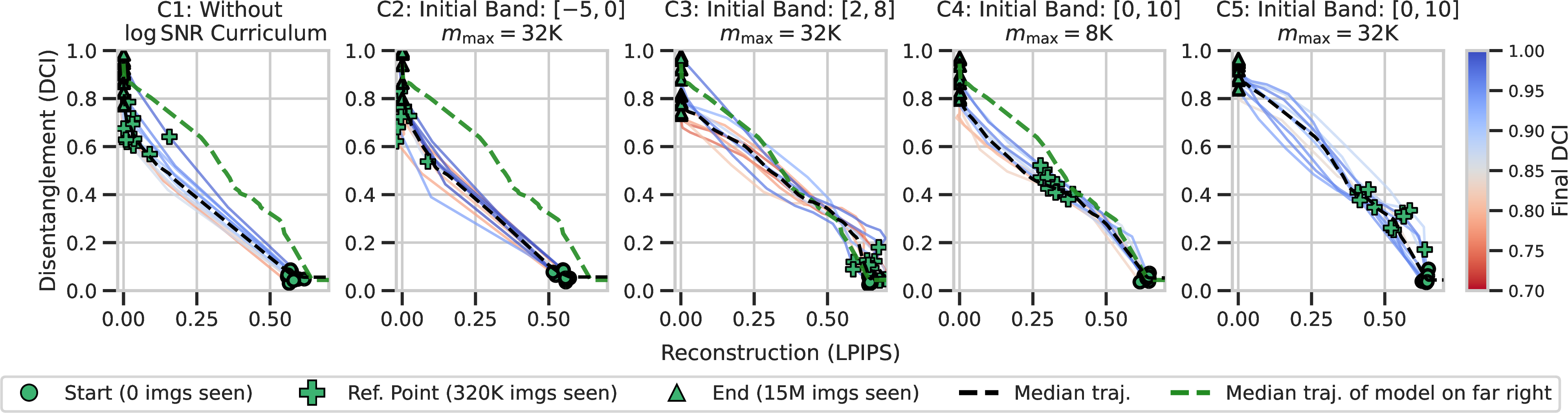
11 shows that all curricula reach similar final reconstruction, with LPIPS saturated at approximately \(0.0005\). The main differences are therefore in representation quality. With a fixed widening duration of \(32\)K, changing the initial band changes the final disentanglement scores: the high-noise initial band \([-5,0]\) gives strong DCI and FactorVAE, while the moderate band \([0,10]\) gives the best overall combination once the widening duration is tuned. For the \([0,10]\) initial band, widening over \(32\)K steps performs best across DCI, FactorVAE, and MIG, whereas faster widening (\(8\)K) and slower widening (\(64\)K) both reduce at least one disentanglement metric. This suggests that curriculum design matters beyond simply delaying access to high or low-noise levels; the rate at which the full objective is introduced also affects the representation learned.
9 shows the corresponding optimisation trajectories for DCI, FactorVAE, and MIG. The trajectories reveal that curricula change the path through reconstruction-disentanglement space before final convergence. In particular, the best-performing curriculum follows a different trajectory, delaying early commitment to a reconstruction-dominated path and reaching high final disentanglement with lower variance across seeds. These results support H2: early noise-level exposure can steer regime selection by changing the relative pace of reconstruction and semantic organisation.
| \(\lambda_{L}(0)\) | \(\lambda_{U}(0)\) | \(m_{\max}\) | LPIPS \(\downarrow\) | DCI \(\uparrow\) | FactorVAE \(\uparrow\) | MIG \(\uparrow\) |
|---|---|---|---|---|---|---|
| \(0\) | \(12\) | \(32\)K | \(0.0005 \pm 0.0000\) | \(0.834 \pm 0.065\) | \(0.935 \pm 0.045\) | \(0.329 \pm 0.097\) |
| \(2\) | \(8\) | \(32\)K | \(0.0005 \pm 0.0000\) | \(0.860 \pm 0.100\) | \(0.941 \pm 0.068\) | \(0.290 \pm 0.097\) |
| \(-5\) | \(0\) | \(32\)K | \(0.0005 \pm 0.0000\) | \(0.914 \pm 0.096\) | \(0.976 \pm 0.039\) | \(0.348 \pm 0.090\) |
| \(0\) | \(10\) | \(8\)K | \(0.0005 \pm 0.0000\) | \(0.883 \pm 0.063\) | \(0.968 \pm 0.050\) | \(0.375 \pm 0.146\) |
| \(0\) | \(10\) | \(32\)K | \(0.0005 \pm 0.0000\) | \(\mathbf{0.926 \pm 0.043}\) | \(\mathbf{0.991 \pm 0.017}\) | \(\mathbf{0.353 \pm 0.056}\) |
| \(0\) | \(10\) | \(64\)K | \(0.0005 \pm 0.0000\) | \(0.864 \pm 0.038\) | \(0.954 \pm 0.046\) | \(0.266 \pm 0.099\) |
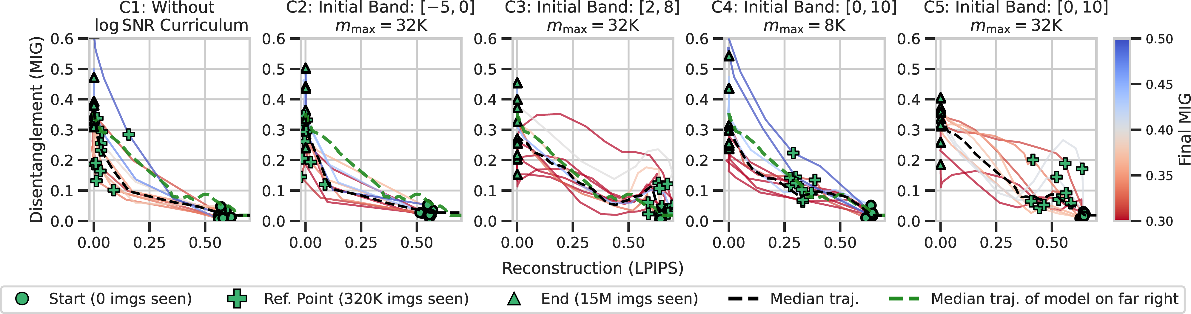
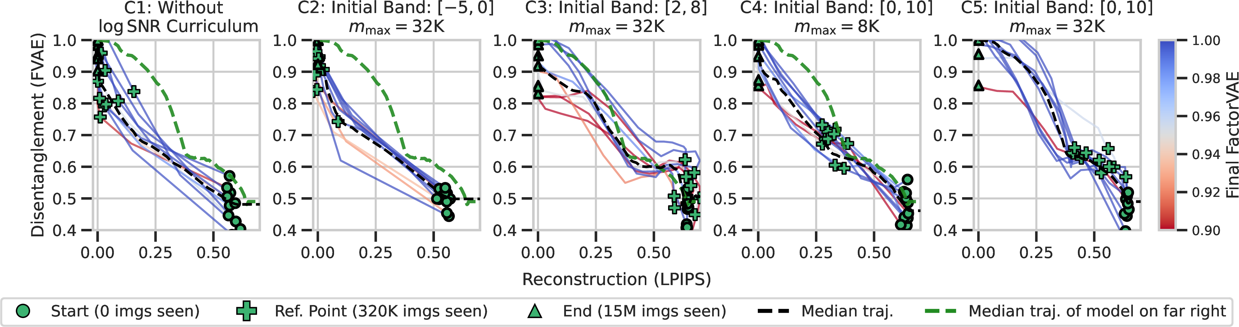
Figure 9: \(\log \mathrm{SNR}\) curricula steer optimisation trajectories across disentanglement metrics. Optimisation trajectories for curriculum ablations on Shapes3D, using DCI, FactorVAE, and MIG as the disentanglement axis. Panels correspond to different curricula; colours indicate final disentanglement, and dashed curves show median trajectories. Changing the initial band and widening duration changes the path through reconstruction–disentanglement space, not just the final score. The moderate curriculum \([0,10]\) with \(m_{\max}=32\)K gives the strongest overall disentanglement, supporting curriculum design as a mechanism for regime selection..
12.7 Attribute Disentanglement↩︎


Figure 10: Latent edits reveal interpretable factors across datasets. Each panel compares EncDiff and SteeringDRL by replacing a single source slot with the corresponding target slot. On
Cars3D, edits capture viewpoint (Azimuth, Elevation) and object identity (Object Type / Style). On Shapes3D with \(N = 10\), we can more consistently perform all edits, whereas EncDiff
often struggles with Floor Hue and Object Shape.. a — Cars3D example 1, b — Cars3D example 2, c — Shapes3D example 1, d — Shapes3D example 2
12.8 Spatial Disentanglement with Object-Centric Learning↩︎
12.8.1 ClevrTex↩︎

| Segmentation | Recon. | Comp. | |||
|---|---|---|---|---|---|
| 2-4 (lr)5-5 (lr)6-6 Method | FG-ARI \(\uparrow\) | mIoU \(\uparrow\) | mBO \(\uparrow\) | LPIPS \(\downarrow\) | FID \(\downarrow\) |
| SLATE | \(62.75 \pm 5.89\) | \(56.41 \pm 4.02\) | \(60.23 \pm 4.01\) | \(0.402 \pm 0.005\) | \(88.73 \pm 5.37\) |
| SlotDiffusion | \(66.85 \pm 3.22\) | \(56.01 \pm 1.98\) | \(60.20 \pm 2.34\) | \(0.173 \pm 0.015\) | \(47.84 \pm 1.36\) |
| SteeringDRL | \(\mathbf{67.82 \pm 1.40}\) | \(\mathbf{59.20 \pm 1.91}\) | \(\mathbf{63.29 \pm 1.87}\) | \(\mathbf{0.164 \pm 0.004}\) | \(\mathbf{44.01 \pm 1.85}\) |