Target-Guided Selective Reweighting for Physics-Informed Neural Network Inverse Problems: A Transfer Learning Approach
July 06, 2026
Abstract
Physics-informed neural networks (PINNs) encounter ill-posed optimization, loss competition, and parameter compensation in partial differential equation (PDE) inverse problems. Transfer learning can reuse representations from source tasks, but direct fine-tuning may introduce negative transfer when dominant physical mechanisms, governing parameters, or observation noise differ between source and target domains: the model achieves low field error yet recovers incorrect target physical parameters. To mitigate, we propose Target-Guided Selective Reweighting PINN (TGSR-PINN), a target-evidence-driven representation correction method for PINN inverse transfer learning. TGSR-PINN transfers only the weights and biases from the source PINN, while target physical parameters are independently initialized; after a short target-adaptation phase, the method computes neuron target scores using first-order Taylor sensitivity and pre-activation variance on fixed scoring batches, and converts evidence associated with low-scoring neurons into continuous weak-adaptation signals via a Gaussian mixture model (GMM) with rank fallback. TGSR-PINN then applies selective soft decay to input weight rows and biases of low-scoring neurons instead of hard pruning or random resetting. In experiments, TGSR-PINN improves target parameter recovery while maintaining comparable field accuracy in the high-Péclet 2D advection-diffusion task and in the Allen–Cahn to Burgers cross-PDE-family transfer task; a 5%-noise reaction–diffusion case provides supplementary evidence under milder source-target mismatch. Ablation studies suggest that neuron target scoring, weak-adaptation signal estimation, layer protection, and selective soft decay jointly contribute to the benefits.
Physics-informed neural networks ,Partial differential equation inverse problems ,Transfer learning ,Negative transfer ,Selective soft decay ,Parameter inversion
1 Introduction↩︎
Partial differential equations (PDEs) are fundamental mathematical tools for describing continuous physical systems, widely used in fluid mechanics, heat and mass transfer, elasticity, electromagnetic fields, reaction–diffusion systems, and biomedical engineering. Classical numerical methods, such as finite difference, finite element, and finite volume methods, have established mature theoretical and engineering frameworks for solving PDE forward problems. These methods typically require known governing equations, boundary conditions, and physical parameters, and solve for the target physical field through mesh discretization. However, in many practical engineering scenarios, researchers face not only forward problems but also inverse problems that require inferring unknown material properties, diffusion coefficients, velocity parameters, source terms, or boundary conditions from limited, sparse, or noisy observation data. Inverse problems are typically ill-posed and exhibit parameter correlations, where small errors in observational data may lead to significant fluctuations in inversion results, and different parameter combinations may produce similar physical field responses. Consequently, PDE inverse problems are not merely numerical solution tasks but also parameter estimation problems influenced by observation noise, physical priors, and optimization procedures.
Physics-informed neural networks provide a unified differentiable modeling framework for both forward and inverse PDE problems [1], [2]. PINNs approximate the unknown physical field using a neural network \(u_{\theta}(x,t)\) and compute PDE residuals through automatic differentiation, incorporating governing equations, initial conditions, boundary conditions, and observational data into the loss function. For inverse problems, unknown physical parameters can serve as trainable variables, optimized simultaneously with network weights and biases, thereby completing field reconstruction and parameter inversion within the same framework. Compared with purely data-driven models, PINNs leverage physical constraints to reduce reliance on large-scale labeled data and are applicable to scenarios with sparse or incomplete observations; meanwhile, the comparative advantages of PINNs over traditional methods such as finite elements in terms of accuracy, computational cost, and problem settings differ [3]. Subsequent research has further integrated PINNs into physics-informed machine learning and scientific machine learning frameworks, advancing their application to complex engineering problems [2], [4], [5]. Recent surveys have also summarized the development and challenges of PINNs from perspectives including loss function design, geometric modeling, and structural engineering applications [6], [7].
Despite their concise formulation and unified modeling advantages, PINN training is not inherently stable. The PINN loss function typically comprises multiple components—PDE residuals, boundary conditions, initial conditions, and observational data errors—which may differ significantly in numerical scale, gradient direction, and convergence speed. Existing studies have analyzed PINN training difficulties and applicability conditions from perspectives of gradient pathology, neural tangent kernel, and theoretical convergence [8]–[10], and further identified that training failure modes and complex loss landscapes increase optimization difficulty [11], [12]. In inverse problems, these difficulties are further amplified. On one hand, observational data are often limited and noisy; on the other hand, the parameters to be inverted may suffer from insufficient identifiability or mutual compensation. Even when a model can reduce PDE residuals or field prediction errors, it may not accurately recover the target physical parameters. Particularly in multi-parameter inversion tasks, the network representation may compensate for incorrect parameters by adjusting field predictions, yielding seemingly reasonable field results while physical parameters remain far from their true values.
To address PINN training difficulties, numerous improvement directions have been proposed, including gradient enhancement and adaptive loss weighting [13]–[15], domain decomposition [16], [17], frequency-domain modeling and augmented Lagrangian training [18], [19], and residual decay or loss-attention-based weight balancing methods [20], [21]. These methods primarily focus on improving convergence stability and prediction accuracy on a single task. In contrast, PINN transfer learning, especially for inverse problems, must additionally consider the impact of source task representations on target parameter recovery. For inverse problems, the value of transfer cannot be judged solely by training speed or field error; it must also be assessed by whether the transferred representation affects the quality of target physical parameter recovery.
The fundamental idea of transfer learning is to leverage knowledge learned from a source task to assist target task training. When source and target tasks share partial physical structures, geometric features, or solution-space patterns, the network weights and hidden representations from the source model can serve as initialization for the target task, reducing training cost from scratch and potentially improving convergence speed and training stability [22]–[24]. Transfer learning has been applied to PINN inverse problems and data-guided inverse problems [23], [24], and extended to structural mechanics simulation, vortex-induced vibration, and complex engineering systems [25], [26]; recent work has also compared full fine-tuning and lightweight fine-tuning PINN transfer strategies [27]. These studies demonstrate that when source and target tasks exhibit strong relevance, the source model can provide an effective starting point for target training.
However, in PINN inverse transfer learning, source model representations are not uniformly beneficial. The source model may contain physical structures useful for the target task, but may also carry source-task biases inconsistent with the target physics. When source and target tasks differ in governing parameters, boundary conditions, observation layouts, noise levels, or dominant physical mechanisms, directly reusing the source model may steer target optimization toward regions detrimental to parameter recovery, thereby creating negative transfer risk [28], [29]. This risk may not be directly observable from field errors. The source model may accelerate target loss reduction and even achieve low field prediction errors, but simultaneously affect parameter recovery through compensation between network representations and physical parameters. Engineering inverse problems such as material characterization, nondestructive testing, and structural load identification all demonstrate that physical parameter recovery is often as important as field reconstruction, or even a more direct task objective [30], [31].
Existing PINN transfer strategies mostly operate at the layer or parameter-block level. For example, full fine-tuning typically copies all network weights and biases from the source model and continues optimization on the target task; frozen-layer methods assume that shallow representations are more general while deep representations are more task-specific; partial-layer transfer selects certain network layers for copying or updating based on preset rules. These strategies are simple to implement and can constitute effective baselines, but their transfer scope is typically predetermined by human judgment before target training, and rarely reassesses whether hidden neurons remain suitable for the current target inverse problem after the model has been exposed to target data. In other words, existing methods more often address “which layers to transfer” or “which parameter blocks to update,” but less often address the finer-grained question after transfer: which hidden neurons receive high values of the neuron target score under current target evidence, and which low-scoring neurons require selective soft decay?
Therefore, from a machine learning perspective, PINN inverse transfer is not merely an initialization problem but a representation adaptation problem under target evidence. For inverse problems, coarse-grained transfer is particularly prone to masking negative transfer: network representations can compensate for incorrect physical parameters through field function fitting, causing field errors and parameter errors to decouple. This paper formulates the research problem as “target-evidence-driven representation correction”: without inheriting source-task physical parameters, the method reassesses transferred hidden representations using target loss, target responses, and neuron sensitivity, and reduces the influence of transfer units with insufficient target support on subsequent target optimization through continuous reweighting. This formulation distinguishes TGSR-PINN from standard PINN fine-tuning, pruning-based compression, and random resetting methods.
This problem is related to neuron importance estimation and pruning research. Taylor saliency and related methods approximate neuron importance through first-order or second-order loss changes and are widely used for model pruning and compression [32]–[34]; selective pruning has also been applied to weaken noise-affected representations in PINN inverse problems [35]. However, our scenario differs: low-scoring neurons after neuron target scoring are not necessarily entirely useless, and hard pruning, sparse subnetwork search (e.g., the lottery ticket hypothesis [36]), or random reinitialization may all destroy reusable source representations, introducing additional perturbation to subsequent optimization. Therefore, this paper adopts selective soft decay—using target-side evidence to estimate weak-adaptation signals and progressively reducing the influence of low-scoring neurons, rather than hard removal or resetting.
Based on these considerations, we propose Target-Guided Selective Reweighting PINN (TGSR-PINN), a target-side representation correction method for PINN inverse transfer learning. The term “Reweighting” in the method name refers to continuous adjustment of hidden representations through target-side evidence assessment, rather than random reinitialization or hard pruning. The core idea is: the source model transfers only neural network representation parameters; the physical parameters to be inverted are not inherited from the source task but are initialized by the target task protocol and updated jointly with network parameters under the target loss. After representation transfer, TGSR-PINN first performs target short adaptation, allowing the transferred representation to be exposed to target observation data, boundary/initial conditions, and PDE constraints. Subsequently, the method performs neuron target scoring based on target loss, combining Taylor sensitivity, pre-activation variance, and multiple fixed scoring batches to obtain neuron target scores. Further, TGSR-PINN converts neuron target scores into weak-adaptation signals through a GMM with rank fallback. Finally, the method maps weak-adaptation signals to continuous decay factors and applies selective soft decay to low-scoring neurons under layer protection constraints. Note: selective soft decay is not hard pruning or random reinitialization—it preserves network topology and only reduces the influence of low-scoring neurons on subsequent target optimization.
Through these designs, TGSR-PINN transforms coarse-grained weight reuse in PINN inverse transfer into a target-evidence-driven representation diagnosis and soft correction process. Throughout this paper, the core terminology follows the chain “neuron target score \(\to\) weak-adaptation signal \(\to\) low-scoring neuron \(\to\) selective soft decay.” The framework focuses not only on final field error but also on physical parameter error, and records target-side adaptation dynamics, parameter changes, layer-wise selective soft decay statistics, and weak-adaptation signal diagnostic information, thereby providing a basis for analyzing where and how transfer corrections occur and their impact on parameter recovery. This paper focuses on inverse transfer scenarios with significant source–target differences, strong parameter coupling, and field errors insufficient to fully represent parameter recovery quality, with particular attention to multi-parameter inversion performance in high-Péclet number two-dimensional advection–diffusion inverse problems.
The main contributions of this paper are as follows:
A target-evidence-driven representation correction framework is proposed for PINN inverse transfer learning. Unlike directly transferring the complete source-task state, TGSR-PINN explicitly transfers only network weights and biases, while target physical parameters are independently initialized by the target task and updated under the target loss. This design focuses the investigation on the impact of transferred representations on parameter recovery.
A neuron-level target scoring mechanism is designed. This mechanism combines first-order Taylor sensitivity and pre-activation variance under the target loss to compute empirical neuron target scores for hidden neurons on fixed scoring batches, providing target-side evidence for subsequent weak-adaptation signal estimation.
A weak-adaptation signal estimation procedure combining GMM and rank fallback is developed. This procedure identifies low-scoring neurons from the intra-layer neuron target score distribution, falls back to rank-based estimation when GMM evidence is insufficient, and maps weak-adaptation signals to selective soft decay factors. Unlike hard pruning, random resetting, or pure magnitude-based pruning, TGSR-PINN preserves network topology and applies selective soft decay only to the weight rows and biases corresponding to low-scoring neurons.
The proposed method is evaluated on high-Péclet number two-dimensional advection–diffusion, Allen–Cahn to Burgers cross-PDE-family transfer, and a 5%-noise reaction–diffusion inverse problem. Mechanism ablation, scoring component scanning, GMM/rank fallback diagnosis, layer-protection analysis, overall intensity matching, selective soft decay mapping ablation, and computational overhead evaluation are further conducted to clarify the empirical advantages and applicability boundaries of TGSR-PINN.
The remainder of this paper is organized as follows. Section 2 presents the PDE inverse problem formulation and the overall framework of TGSR-PINN. Section 3 presents the experimental design and results, including high-Péclet advection–diffusion, cross-PDE-family transfer, 5%-noise reaction–diffusion experiments, and high-Péclet mechanism ablation and layer-wise diagnosis. Section 4 discusses the relationship between field and parameter errors, the selective soft decay mechanism, computational overhead, and applicability boundaries. Section 5 concludes the paper and outlines future research directions.
2 Method↩︎
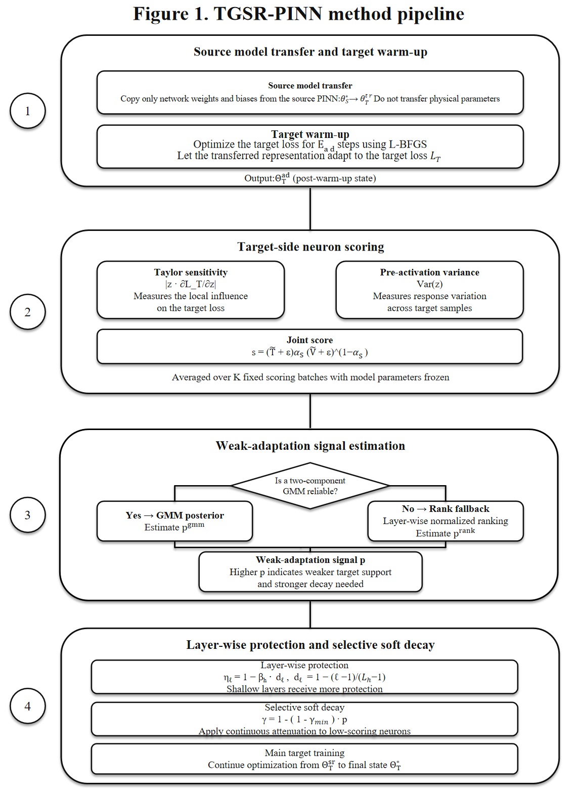
Figure 1 illustrates the overall pipeline of TGSR-PINN. The method first copies the network weights and biases from the source model and independently initializes target physical parameters; then performs short adaptation on the target task, computing neuron target scores using Taylor sensitivity and pre-activation variance under the target loss; estimates weak-adaptation signals via GMM with rank fallback and performs selective soft decay under layer protection constraints; and finally continues from the corrected state to complete target main training.
2.1 PINN Inverse Problem Formulation↩︎
We first present the general PINN formulation for PDE inverse problems. Consider a physical system defined on a spatial domain \(\Omega\) and a temporal interval \([0,T]\). We directly use spatial coordinates \(x\) and time \(t\) as network inputs; for steady-state problems, the time variable \(t\) can be omitted. Let \(u(x,t)\) denote the physical field to be solved and \(\lambda\) denote the physical parameters to be inverted. The general governing equation, boundary conditions, and initial conditions can be written as: \[\mathcal{N}\!\left[ u(x,t);\lambda \right] = f(x,t), \label{eq:pde}\tag{1}\] \[\mathcal{B}\!\left[ u(x,t);\lambda \right] = g(x,t), \label{eq:bc}\tag{2}\] \[u(x,0) = u_{0}(x), \label{eq:ic}\tag{3}\] where Eq. (1 ) holds on \(\Omega \times (0,T]\), Eq. (2 ) holds on \(\partial\Omega \times [0,T]\), and Eq. (3 ) gives the initial state. \(\mathcal{N}[\cdot]\) denotes the PDE differential operator, \(\mathcal{B}[\cdot]\) denotes the boundary operator, \(f(x,t)\) is the source term, and \(g(x,t)\) and \(u_{0}(x)\) denote boundary conditions and initial conditions, respectively. In inverse problems, \(\lambda\) is the unknown parameter to be identified from limited observational data and physical constraints, which may represent diffusion coefficients, reaction coefficients, velocity parameters, material properties, or other physical quantities.
PINNs approximate the unknown physical field \(u(x,t)\) using a fully connected neural network \(u_{\theta}(x,t)\), where \(\theta\) denotes the network parameters including weight matrices and bias vectors for each layer. For the target inverse problem, the physical parameters to be inverted are denoted \(\lambda_{T}\), and the target network parameters are denoted \(\theta_{T}\). Together they constitute the trainable variables \(\Theta_{T}=\{\theta_{T},\lambda_{T}\}\) in the target task and are simultaneously updated under the target loss function.
Substituting the neural network prediction \(u_{\theta_{T}}(x,t)\) into the governing equation yields the PDE residual for the target task: \[r\!\left( x,t;\Theta_{T} \right) = \mathcal{N}\!\left[ u_{\theta_{T}}(x,t);\lambda_{T} \right] - f(x,t). \label{eq:residual}\tag{4}\]
The total loss for the target inverse problem is a weighted sum of components: \[\begin{align} \mathcal{L}_{T}\!\left( \Theta_{T} \right) &= \omega_{pde}\mathcal{L}_{pde} + \omega_{ic}\mathcal{L}_{ic} \\ &\quad + \omega_{bc}\mathcal{L}_{bc} + \omega_{data}\mathcal{L}_{data}. \end{align} \label{eq:loss}\tag{5}\] where \(\omega_{pde}\), \(\omega_{ic}\), \(\omega_{bc}\), and \(\omega_{data}\) are the weights for each loss term. The focus of this paper is on how the transferred network representation is continuously corrected based on target-task evidence. Section 2.2 will describe how TGSR-PINN reduces the influence of low-scoring neurons on target optimization through selective soft decay, thereby avoiding the excessive perturbation caused by random resetting.
2.2 Overall Framework of TGSR-PINN↩︎
To avoid terminological confusion, we define TGSR-PINN as Target-Guided Selective Reweighting PINN. Here, Target-Guided means that scoring evidence comes from the target task’s loss, sampling batches, gradients, and pre-activation responses; Selective means that only low-scoring neurons are processed; and selective soft decay / reweighting means that the corresponding weight rows and biases are continuously scaled, rather than randomly reset, hard-pruned, or neurons removed. For consistency, the following sections use “neuron target score” for the target-side evidence obtained from Taylor sensitivity and pre-activation variance, “weak-adaptation signal” for the continuous decay signal derived from neuron target scores, “low-scoring neurons” for the neuron objects to be weakened, and “selective soft decay” for the final weight-row and bias scaling operation.
Notation Summary↩︎
| Symbol | Meaning |
|---|---|
| \(\theta_{S}^{*}\) | Source network representation parameters (weights and biases) after source training |
| \(\theta_{T}^{tr}\) | Target initial network parameters copied from the source model |
| \(\lambda_{T}^{0}\) | Target physical parameter initial values, independently initialized |
| \(\Theta_{T}^{0}\) | Target initial state: transferred network parameters and target parameter init |
| \(\Theta_{T}^{ad}\) | State after target short adaptation, containing \(\theta_{T}^{ad}\) and \(\lambda_{T}^{ad}\) |
| \(\Theta_{T}^{sr}\) | Target state after selective soft decay |
| \(\Theta_{T}^{*}\) | Final target state after main training |
| \(\mathcal{L}_{T}\) | Target inverse loss (PDE, BC/IC, and data error) |
| \(E_{ad},\; E_{main}\) | Target short adaptation steps and subsequent main training steps |
| \(K,\; B_{k}^{score}\) | Number of scoring batches and \(k\)-th scoring batch |
| \(z_{\ell,j}^{(k)}\) | Pre-activation of neuron \(j\) in layer \(\ell\) on batch \(k\) |
| \(T_{\ell,j}^{(k)},\; V_{\ell,j}^{(k)}\) | Taylor sensitivity and pre-activation variance |
| \(s_{\ell,j}^{(k)},\; s_{\ell,j}\) | Per-batch and multi-batch averaged neuron target score |
| \(x_{\ell,j}\) | Compressed intra-layer neuron target score |
| \(q_{\ell,j}^{L}\) | Posterior responsibility of neuron to GMM low-mean component |
| \(p_{\ell,j},\; \widetilde{p}_{\ell,j}\) | Weak-adaptation signal (before/after layer protection) |
| \(c_{\ell}\) | GMM two-component separation confidence |
| \(\beta_h,\; \eta_{\ell},\; d_{\ell}\) | Shallow protection strength, layer protection coefficient, layer position factor |
| \(\mathcal{M}_{\ell}\) | Diagnostic set of neurons effectively affected by selective soft decay in layer \(\ell\) |
| \(\gamma_{\ell,j},\; \gamma_{m},\; \gamma_{\min}\) | Neuron scaling factor, intermediate and minimum scaling factors |
| \(W_{\ell,j:},\; b_{\ell,j}\) | Input weight row and bias for neuron \(j\) in layer \(\ell\) |
| \(\alpha_{s},\; \Delta_{\alpha}\) | Base fusion weight and layer-wise increment for Taylor/variance |
| \(\xi,\; \rho_{r},\; \delta_{g}\) | Rank fallback max signal, rank power exponent, selective soft decay threshold |
Numerical stability constants are defined when introduced: \(\varepsilon=10^{-6}\) is used in Eq. (11 ) and layer-wise normalization; \(\varepsilon_s\), \(\varepsilon_p\), and \(\varepsilon_r\) are set to \(10^{-12}\) in Eqs. (13 ), (16 ), and (17 ), respectively. The GMM variance floor is \(10^{-10}\).
TGSR-PINN starts from the following transfer setting: the source model provides only neural network representation parameters, and target physical parameters are independently initialized by the target task. This setting follows the fundamental principle in transfer learning of reusing transferable representations while avoiding direct inheritance of mismatched task states. Source-task physical parameters, optimizer states, training history, and sampling batches are all not transferred. Let \(\theta_{S}^{*}\) denote the network parameters after source training; then the target network is initialized as \[\theta_{T}^{tr} \leftarrow \theta_{S}^{*},\quad \Theta_{T}^{0} = \{\theta_{T}^{tr},\lambda_{T}^{0}\}. \label{eq:init}\tag{6}\] where \(\lambda_{T}^{0}\) is the initial value of the target physical parameter. This setting ensures that the comparison focuses on transferred representations and their correction mechanisms, rather than direct inheritance of source-task physical parameters.
Subsequently, starting from \(\Theta_{T}^{0}\), the model performs \(E_{ad}\) steps of target short adaptation under the target loss \(\mathcal{L}_{T}\). This stage simultaneously updates the transferred network parameters \(\theta_{T}^{tr}\) and the target physical parameters \(\lambda_{T}^{0}\), yielding the post-adaptation state: \[\Theta_{T}^{ad} = \{\theta_{T}^{ad},\lambda_{T}^{ad}\} = \mathrm{Train}\!\left( \Theta_{T}^{0},\mathcal{L}_{T},E_{ad} \right). \label{eq:adapt}\tag{7}\] The target short adaptation is positioned as a short training phase before neuron target scoring, whose role is to expose the copied network weights and biases to target observation data, boundary/initial conditions, and PDE constraints. Thus, subsequent neuron target scoring is based on the state \(\Theta_{T}^{ad}\) after the model has acquired preliminary target responses, rather than directly on the source-task state. In implementation, the short-adaptation step count is chosen by the target training budget proportion and a short-adaptation upper bound. If this phase is too long or the initial physical parameters deviate severely from true values, the scoring signal may also be contaminated by early erroneous parameter compensation; therefore, we treat the short-adaptation length as a proportional control and report its sensitivity analysis in experiments.
After completing target short adaptation, TGSR-PINN temporarily fixes \(K\) scoring batches from the target training sampler: \[\mathcal{B}_{score} = \{ B_{1}^{score},B_{2}^{score},\ldots,B_{K}^{score}\}. \label{eq:batch}\tag{8}\] Each scoring batch is consistent with the sample types in the target loss, including PDE collocation points, boundary condition points, initial condition points, and observation data points. If a task does not include a certain constraint type, the scoring batch does not include the corresponding samples either. Unless overridden by configuration, the experimental implementation defaults to \(K=3\). During the scoring phase, the model state is fixed at \(\Theta_{T}^{ad}\), i.e., the post-adaptation network parameters \(\theta_{T}^{ad}\) and target physical parameters \(\lambda_{T}^{ad}\) are frozen. This phase performs only forward computation and gradient backpropagation to collect hidden neuron pre-activation responses, target loss gradients, and pre-activation variance information; no optimizer updates are executed. After scoring, these cached batches no longer participate as fixed constraints in subsequent training, and the model continues sampling and optimizing according to the original target training protocol.
Consider the \(j\)-th hidden neuron in the \(\ell\)-th layer. In our implementation, hooks are registered at the linear output of each fully connected layer, so we denote its pre-activation response on the \(k\)-th scoring batch as \(z_{\ell,j}^{(k)}(x,t)\). To approximately measure the neuron’s local contribution to the target loss, we introduce a virtual gating variable \(g_{\ell,j}\), writing the pre-activation as \(g_{\ell,j}z_{\ell,j}^{(k)}(x,t)\). During normal forward computation, \(g_{\ell,j} = 1\); perturbing it to 0 can be approximately understood as suppressing that neuron’s input response. This scoring idea is consistent with Taylor-expansion-based neuron importance estimation for pruning [32]. Based on the first-order Taylor expansion, the Taylor sensitivity on the \(k\)-th scoring batch is defined as \[T_{\ell,j}^{(k)} = \mathbb{E}_{(x,t) \in B_{k}^{score}}\left| z_{\ell,j}^{(k)}(x,t)\frac{\partial\mathcal{L}_{T}^{(k)}}{\partial z_{\ell,j}^{(k)}(x,t)} \right|. \label{eq:taylor}\tag{9}\]
Taylor sensitivity reflects the first-order sensitivity of the target loss to this neuron’s pre-activation response. A larger value indicates that changes in the neuron’s pre-activation have a more pronounced effect on the current target loss; the absolute value in Eq. (9 ) prevents positive and negative gradient directions from canceling each other.
Relying solely on Taylor sensitivity may be affected by local gradient fluctuations. Some neurons may have large gradients on specific batches but weak response variation on target samples. Therefore, TGSR-PINN simultaneously computes pre-activation variance: \[V_{\ell,j}^{(k)} = \mathrm{Var}_{(x,t) \in B_{k}^{score}}\!\left( z_{\ell,j}^{(k)}(x,t) \right). \label{eq:variance}\tag{10}\] Here, the variance specifically refers to the pre-activation variance of the linear layer output \(z_{\ell,j}\), not the variance of the post-activation value \(\tanh(z_{\ell,j})\). We use pre-activation statistics because the hooks in our implementation are registered at the linear layer output, and subsequent selective soft decay directly modulates the pre-activation magnitude by scaling \(W_{\ell,j:}\) and \(b_{\ell,j}\). Deep network initialization and normalization research has long focused on the mean and variance of layer inputs or neuron summed inputs to maintain signal propagation and training stability [37]–[39]. Thus, pre-activation variance characterizes the linear response variation range of the neuron on target samples and serves as an auxiliary statistic for target sample response activity in neuron target scoring.
Since numerical scales may differ across layers, we first normalize \(T_{\ell,j}^{(k)}\) and \(V_{\ell,j}^{(k)}\) within each layer separately, obtaining \(\widetilde{T}_{\ell,j}^{(k)}\) and \(\widetilde{V}_{\ell,j}^{(k)}\). The implementation uses layer-wise z-score, negative-value truncation, and maximum rescaling to bring both types of evidence into \([0,1]\). Let \(L_h\) denote the number of hidden layers. Before geometric fusion, we define \(\alpha_{\ell}=\alpha_s+\Delta_{\alpha}(\ell-1)/(L_h-1)\) to control the relative weight of Taylor sensitivity and pre-activation variance in layer \(\ell\); for a single hidden layer, we set \(\alpha_{\ell}=\alpha_s+\Delta_{\alpha}/2\). We then compute the neuron target score for this batch using geometric fusion: \[s_{\ell,j}^{(k)} = \left( \widetilde{T}_{\ell,j}^{(k)} + \varepsilon \right)^{\alpha_{\ell}}\!\left( \widetilde{V}_{\ell,j}^{(k)} + \varepsilon \right)^{1 - \alpha_{\ell}}. \label{eq:score95single}\tag{11}\] where \(\varepsilon=10^{-6}\) is the numerical stability term in Eq. (11 ). The experimental defaults are \(\alpha_s=0.5\) and \(\Delta_{\alpha}=0.3\), so deeper neurons score more toward Taylor sensitivity. Compared with arithmetic averaging, this geometric fusion is more sensitive to the smaller of the two evidence terms: if either Taylor sensitivity or pre-activation variance is weak, the neuron target score is suppressed. This prevents a neuron from being judged strongly target-relevant solely because of a single large gradient or a single large response magnitude. Averaging over \(K\) scoring batches yields the neuron target score for neuron \(j\) in layer \(\ell\): \[s_{\ell,j} = \frac{1}{K}\sum_{k = 1}^{K}s_{\ell,j}^{(k)}. \label{eq:score95avg}\tag{12}\] A higher \(s_{\ell,j}\) indicates stronger target evidence supporting retention of the neuron; a lower neuron target score indicates weaker target evidence support, and the subsequent continuous weak-adaptation signal will determine the selective soft decay intensity.
After obtaining neuron target scores \(s_{\ell,j}\), TGSR-PINN avoids fixed-threshold binary classification because score scales and distribution shapes vary significantly across layers. We convert neuron target scores to weak-adaptation signals \(p_{\ell,j}\): higher \(s_{\ell,j}\) means the current target evidence better supports retaining the neuron, while higher \(p_{\ell,j}\) means the neuron requires more weakening. To reduce the influence of extreme high scores on distribution estimation, we first apply a compression transform to each layer’s neuron target scores: \[\begin{align} r_{\ell} &= \mathrm{median}\!\left\{s_{\ell,j}:s_{\ell,j}>0\right\} + \varepsilon_{s},\\ x_{\ell,j} &= \log\!\left(1+\frac{s_{\ell,j}}{r_{\ell}}\right). \end{align} \label{eq:compress}\tag{13}\] where \(r_{\ell}\) is the robust scale for layer \(\ell\) and \(\varepsilon_{s}=10^{-12}\) is a numerical stability term.
Subsequently, a one-dimensional two-component GMM is fit on each layer’s \(x_{\ell,j}\), with parameters estimated via the EM algorithm [40]: \[\begin{align} f_{\ell}(x) &= \pi_{\ell,L} \mathcal{N}\!\left( x;\mu_{\ell,L},\sigma_{\ell,L}^{2} \right)\\ &\quad + \pi_{\ell,H} \mathcal{N}\!\left( x;\mu_{\ell,H},\sigma_{\ell,H}^{2} \right). \end{align} \label{eq:gmm}\tag{14}\] where the lower-mean component \(L\) represents the candidate low-scoring-neuron component and the higher-mean component \(H\) represents the relatively high-scoring-neuron component. For neuron \(j\), its posterior responsibility to the low-mean component is \[q_{\ell,j}^{L} = \frac{\pi_{\ell,L}\mathcal{N}\!\left( x_{\ell,j};\mu_{\ell,L},\sigma_{\ell,L}^{2} \right)}{f_{\ell}\!\left( x_{\ell,j} \right)}. \label{eq:responsibility}\tag{15}\]
To make it more suitable for subsequent selective soft decay, we calibrate it to obtain the GMM branch’s weak-adaptation signal: \[p_{\ell,j}^{gmm} = c_{\ell}\cdot \mathrm{clip}\!\left( \frac{q_{\ell,j}^{L} - \pi_{\ell,L}}{1 - \pi_{\ell,L} + \varepsilon_{p}},0,1 \right). \label{eq:gmm95signal}\tag{16}\] where \(c_{\ell}\in[0,1]\) is the separation confidence derived from the two-component overlap and \(\varepsilon_p=10^{-12}\) is a numerical stability term; in implementation, \(c_{\ell}=1-BC_{\ell}\), where \(BC_{\ell}\) is the Bhattacharyya coefficient [41] between the two Gaussian components. The stronger the overlap between the two components, the smaller \(c_{\ell}\) becomes, making the weak-adaptation signal from the GMM branch more conservative. In Eq. (16 ), \(q_{\ell,j}^{L}-\pi_{\ell,L}\) denotes the posterior excess of the low-mean component responsibility over its layer-wise prior weight. Only posterior evidence exceeding this prior is converted into a weak-adaptation signal, which avoids interpreting a large low-scoring component as an anomalous subgroup requiring strong selective soft decay. The GMM branch uses distributional information when the intra-layer neuron target score distribution contains a clear low-scoring-neuron cluster, while rank fallback provides a conservative alternative when GMM evidence is insufficient.
For implementation, TGSR-PINN fits the GMM to the compressed scores \(\log(1+s/r_{\ell})\) in Eq. (13 ). The two component means are initialized at the 25th and 75th percentiles of the compressed scores, the mixture weights are initialized to 0.5, the variance floor is set to \(10^{-10}\), and EM runs for at most 100 iterations with convergence declared when the log-likelihood change is below \(10^{-8}\). We define \(\Delta \mathrm{BIC}=\mathrm{BIC}_{1G}-\mathrm{BIC}_{2G}\), where \(\mathrm{BIC}_{1G}\) is the BIC of the single-Gaussian model and \(\mathrm{BIC}_{2G}\) is the BIC of the two-component GMM. Since lower BIC is better, \(\Delta \mathrm{BIC}>0\) indicates that the two-component model is preferred over the single-Gaussian model. In implementation, we use \(\Delta \mathrm{BIC}>10\) and \(\pi_{\ell,L}\leq 0.5\) as the primary conditions for enabling the GMM branch [42]. The constraint \(\pi_{\ell,L}\leq 0.5\) ensures that the low-mean component represents a minority group of low-scoring neurons within the layer rather than the majority component. If the conditions are not met, the GMM branch is abandoned and rank fallback is activated: \[p_{\ell,j}^{rank} = \xi \cdot \left(\frac{n_{\ell} - \mathrm{rank}_{\ell}(s_{\ell,j})}{n_{\ell} - 1 + \varepsilon_{r}}\right)^{\rho_{r}}. \label{eq:rank}\tag{17}\] where \(\xi=0.75\), \(\rho_r=1.5\), and \(\varepsilon_r=10^{-12}\).
To prevent excessive intervention on shallow input representations, we first apply layer protection to the weak-adaptation signals. With \(L_{h}\) hidden layers: \[\begin{align} d_{\ell} &= 1-\frac{\ell-1}{L_{h}-1},\\ \eta_{\ell} &= 1-\beta_{h}d_{\ell},\\ \widetilde{p}_{\ell,j} &= \mathrm{clip}\!\left(\eta_{\ell}p_{\ell,j},0,1\right). \end{align} \label{eq:layer95protect}\tag{18}\] where \(\beta_h=0.55\) is the shallow protection strength [29]. For a single-hidden-layer network, we set \(d_{\ell}=1\).
Based on the adjusted weak-adaptation signal \(\widetilde{p}_{\ell,j}\), TGSR-PINN maps it directly to a continuous scaling coefficient: \[\begin{align} \gamma_{\ell,j} &= \begin{cases} 1 - A_{\ell,j}(1-\gamma_{m}), & \widetilde{p}_{\ell,j}<0.5,\\ \gamma_{m} - B_{\ell,j}(\gamma_{m}-\gamma_{\min}), & \widetilde{p}_{\ell,j}\geq 0.5, \end{cases}\\ A_{\ell,j} &= \left(2\widetilde{p}_{\ell,j}\right)^3,\\ B_{\ell,j} &= \left(2\widetilde{p}_{\ell,j}-1\right)^3. \end{align} \label{eq:decay95map}\tag{19}\] where \(0\leq\widetilde{p}_{\ell,j}\leq1\), \(\gamma_{m}=0.85\), and \(\gamma_{\min}=0.4\). This mapping is used as a monotone, continuous, and lower-bounded selective scaling rule; it provides mild selective soft decay for moderate weak-adaptation signals and stronger but still recoverable selective soft decay for pronounced weak-adaptation signals. Its motivation is consistent with soft pruning and soft-threshold sparsification, which preserve network capacity and avoid irreversible deletion [43]–[45]. Section 3.5 further compares this default mapping with linear, sigmoid, and hard-threshold alternatives.
For reporting and visualization, we define the diagnostic set of effectively softened neurons as \[\mathcal{M}_{\ell}=\{j:1-\gamma_{\ell,j}\geq\delta_g\}, \label{eq:softened95set}\tag{20}\] where \(\delta_g=0.02\) is only a reporting threshold. The actual operation is still the continuous scaling by \(\gamma_{\ell,j}\), rather than hard deletion or random resetting based on \(\mathcal{M}_{\ell}\).
Selective soft decay is written as \[W_{\ell,j:} \leftarrow \gamma_{\ell,j}W_{\ell,j:},\quad b_{\ell,j} \leftarrow \gamma_{\ell,j}b_{\ell,j}. \label{eq:soft95decay}\tag{21}\] Let \(z_{\ell,j}=W_{\ell,j:}h_{\ell-1}+b_{\ell,j}\). At the instant when Eq. (21 ) is applied, for a fixed previous-layer input \(h_{\ell-1}\), the updated pre-activation satisfies \(z'_{\ell,j}=\gamma_{\ell,j}z_{\ell,j}\). Therefore, Eq. (21 ) is consistent with the virtual pre-activation gate used for scoring in Eq. (9 ) at the pre-activation level: both correspond to multiplicative modulation of \(z_{\ell,j}\). It should be distinguished from a post-activation gate \(\gamma_{\ell,j}\tanh(z_{\ell,j})\) and from outgoing weight scaling in the next layer. Under nonlinear activations such as tanh, scaling the pre-activation is not exactly equivalent to linearly scaling the activation output. We adopt weight-row and bias scaling because it requires no additional network modules or permanent masks and matches the parameterization used in the implementation.
Since \(\gamma_{\min}>0\), Eq. (21 ) does not remove neurons or alter network topology. The selectively decayed weights and biases remain trainable in subsequent main training, so low-scoring neurons can still recover if later target optimization makes them useful. Denoting the post-decay target state as \[\Theta_{T}^{sr}=\mathcal{S}(\Theta_{T}^{ad};\{\gamma_{\ell,j}\}), \label{eq:state95sr}\tag{22}\] the model finally continues training to obtain: \[\Theta_{T}^{*} = \mathrm{Train}(\Theta_{T}^{sr},\mathcal{L}_{T},E_{main}). \label{eq:final}\tag{23}\] This completes the full TGSR-PINN pipeline from source representation transfer, target short adaptation, neuron target scoring, weak-adaptation signal estimation, to selective soft decay and target main training.
2.3 Algorithm Overview↩︎
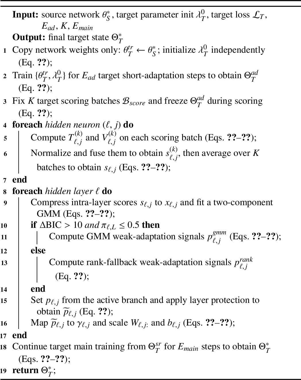
Algorithm 2 summarizes the main steps of TGSR-PINN.
3 Experimental Design and Results↩︎
3.1 Overall Protocol, Evaluation Metrics, and Figure Arrangement↩︎
The baseline methods compared in this paper include:
PINNs: No source model; target task trained from random initialization;
Full Fine-Tuning: All source weights and biases copied and updated;
Lightweight Fine-Tuning: Earlier layers frozen, only later layers updated;
Partial Transfer: Only selected network layers transferred;
TL-gPINN: Transfer learning combined with gradient-enhanced PINN;
BitFit: Only bias terms are trained.
Evaluation metrics include relative \(L_2\) field error and average parameter error, both reported as percentages. The former represents the relative \(L_2\) error of the predicted physical field with respect to the true solution, while the latter denotes the mean of the relative errors of the physical parameters to be inverted. For multi-parameter inversion tasks, the average parameter error is the arithmetic mean of the absolute relative errors of each physical parameter and is therefore non-negative. Since field error and parameter error may not be consistent in PINN inverse problems, we report both metrics simultaneously and focus on parameter recovery quality in the main experiments.
All main experimental tasks employ multiple random repetition protocols. The main text reports aggregated results and key representative repetitions; complete settings and raw results are preserved as reproduction materials. During training, the LBFGS stage uses a fixed-sampling-batch early stopping rule: if the relative improvement in total loss falls below \(10^{-8}\) for consecutive rounds, that repetition terminates early. This early stopping condition depends only on training loss and does not use true physical parameter errors or test field errors as stopping criteria, thus avoiding leakage of true label information into the training process.
To reduce the influence of random initialization, observation sampling, and optimization path differences on conclusions, we adopt a paired comparison protocol based on matched repetitions wherever possible. For different transfer strategies within the same task, if they share the matched initialization protocol, observation data pool, collocation points, and training budget, the final field and parameter errors are treated as paired samples. The main text uses the mean \(\pm\) standard deviation across repetitions as the primary evidence; the best repetition is used for representative mechanism diagnosis and parameter recovery potential analysis, while core conclusions still rely on aggregated statistics from multiple repetitions.
3.2 High-Péclet Number 2D Advection–Diffusion Inverse Problem↩︎
The source task is a 2D diffusion inverse problem (infer \(\alpha\), 0.5% noise, \(\alpha\) init 0.1, true 0.001): \[u_{t} - \alpha(u_{xx} + u_{yy}) = Q_{S}(x,y,t).\] The target task introduces directional advection on the diffusion structure: \[\begin{align} u_{t} - \alpha(u_{xx} + u_{yy}) + v_{x}u_{x} + v_{y}u_{y} &= Q_{T}(x,y,t),\\ \text{infer}\quad &\alpha,v_{x},v_{y}. \end{align}\]
The Péclet number is defined as \(Pe = UL/\alpha\), with \(L=1\), \(U=\sqrt{v_x^2+v_y^2}=\sqrt{5}\), and \(\alpha=0.001\), yielding \(Pe \approx 2.24\times 10^3\), indicating a strongly advection-dominated regime.
| Item | Setting |
|---|---|
| PDE | \(u_t-\alpha(u_{xx}+u_{yy})+v_xu_x+v_yu_y=Q_T\) |
| Domain | \(\Omega=[0,1]^2\), \(t\in[0,1]\) |
| Reference | Manufactured solution \(u=e^{-t}\sin(\pi x)\sin(\pi y)\) |
| Boundary / IC | Homogeneous Dirichlet boundaries induced by the manufactured solution; \(u(x,y,0)=\sin(\pi x)\sin(\pi y)\) |
| Unknown params | \(\alpha\), \(v_x\), \(v_y\) |
| True params | \(\alpha=0.001\), \(v_x=2.0\), \(v_y=1.0\) |
| Init params | \(\alpha=0.005\), \(v_x=1.0\), \(v_y=0.5\) |
| Noise | 0.5% on target observations |
| Sampling / batches | PDE 10000, BC 2500, IC 2500, data 1000 |
| Loss weights | \(\omega_{pde}=10\), \(\omega_{ic}=10\), \(\omega_{bc}=10\), \(\omega_{data}=50\) |
| Network | MLP \([3,100^6,1]\), tanh, LBFGS 300 epochs |
| Péclet | \(Pe\approx2.24\times10^3\) |
| Method | \(n\) | \(L_2\) error (%) | Param error (%) | Time (s) |
|---|---|---|---|---|
| PINNs | 7 | \(0.134 \pm 0.038\) | \(14.825 \pm 6.021\) | 252 |
| Full FT | 7 | \(0.088 \pm 0.018\) | \(6.582 \pm 3.314\) | 235 |
| Lightweight FT | 7 | \(0.087 \pm 0.011\) | \(4.825 \pm 2.384\) | 232 |
| Partial Transfer | 7 | \(0.129 \pm 0.027\) | \(13.906 \pm 4.332\) | 242 |
| TL-gPINN | 7 | \(0.091 \pm 0.022\) | \(7.430 \pm 3.320\) | 552 |
| BitFit | 7 | \(0.184 \pm 0.035\) | \(7.137 \pm 4.754\) | 160 |
| TGSR-PINN | 7 | \(\mathbf{0.080 \pm 0.016}\) | \(\mathbf{4.426 \pm 3.019}\) | 266 |
Table 3 shows that TGSR-PINN achieves the lowest average field error and average parameter error among all compared methods in the high-Péclet setting. Compared with Full Fine-Tuning, TGSR-PINN reduces the average parameter error from 6.582% to 4.426% while maintaining a slightly lower field error. Compared with Lightweight FT, the field errors are close, but TGSR-PINN still obtains a lower average parameter error. These results indicate that the proposed target-side representation correction is more effective for parameter recovery than direct fine-tuning or simple layer freezing in this inverse transfer setting.
| Method | Best \(\alpha\) error (%) |
|---|---|
| PINNs | 14.63 |
| Full FT | 10.68 |
| Lightweight FT | 4.06 |
| Partial Transfer | 24.25 |
| TL-gPINN | 11.63 |
| BitFit | 4.09 |
| TGSR-PINN | 0.38 |
The advection velocities \(v_{x}\) and \(v_{y}\) are non-discriminative for all methods (\(<\)0.03%); the real challenge lies in the diffusion coefficient \(\alpha\). Therefore, Table 4 reports only the best \(\alpha\) error across random repetitions for each method, to show parameter recovery potential, while the overall performance ranking is based on the multi-repetition mean \(\pm\) standard deviation in Table 3. TGSR-PINN achieves the best \(\alpha\) error of 0.38%, while the best non-TGSR baseline (Lightweight FT) achieves 4.06%. This result indicates that target-side representation correction can help recover key physical parameters in challenging advection-dominated inverse problems. BitFit’s average parameter error of 7.137% is close to Full FT’s 6.582%, indicating that bias-only adjustment can partially mitigate transfer error; however, its best \(\alpha\) repetition is 4.09%, still significantly higher than TGSR-PINN’s 0.38%. This comparison suggests that for physical parameters like \(\alpha\) that are deeply coupled with network representation structure, bias-only updates have limited recovery capability, while target-side neuron-level representation correction can more effectively improve parameter inversion quality.
Multiple random repetition results show that the high-Péclet task is TGSR-PINN’s most concentrated advantage scenario. Among the methods fully comparable in the main experiment, TGSR-PINN achieves the lowest relative \(L_2\) field error and lowest average parameter error (L2 0.080%, param 4.426%). BitFit’s field error of 0.184% is also relatively low, and its parameter mean is close to Lightweight FT, indicating that parameter-efficient fine-tuning can be competitive in some inverse transfer scenarios; however, its larger cross-repetition fluctuation in \(\alpha\) recovery further shows that inverse transfer cannot be evaluated solely by field error, nor by comparing only means while ignoring parameter-level stability. Table 4 further reveals TGSR-PINN’s \(\alpha\) recovery advantage (best repetition: 0.38%). To supplement the tabular statistics, Figure 3 shows training loss evolution, Figure 4 presents convergence of average parameter error and three individual parameter errors, and Figure 5 compares the true field and absolute error maps at the \(t=1\) cross-section.
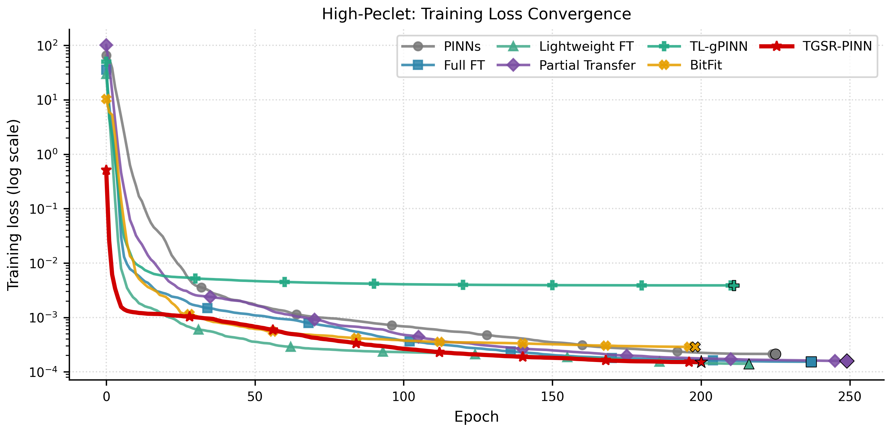
Figure 3 shows that TGSR-PINN reaches a low training loss while avoiding the unstable plateau observed in TL-gPINN. Although the final training loss alone does not fully determine parameter accuracy, the curve indicates that the proposed soft-decay correction does not destabilize the target optimization process.
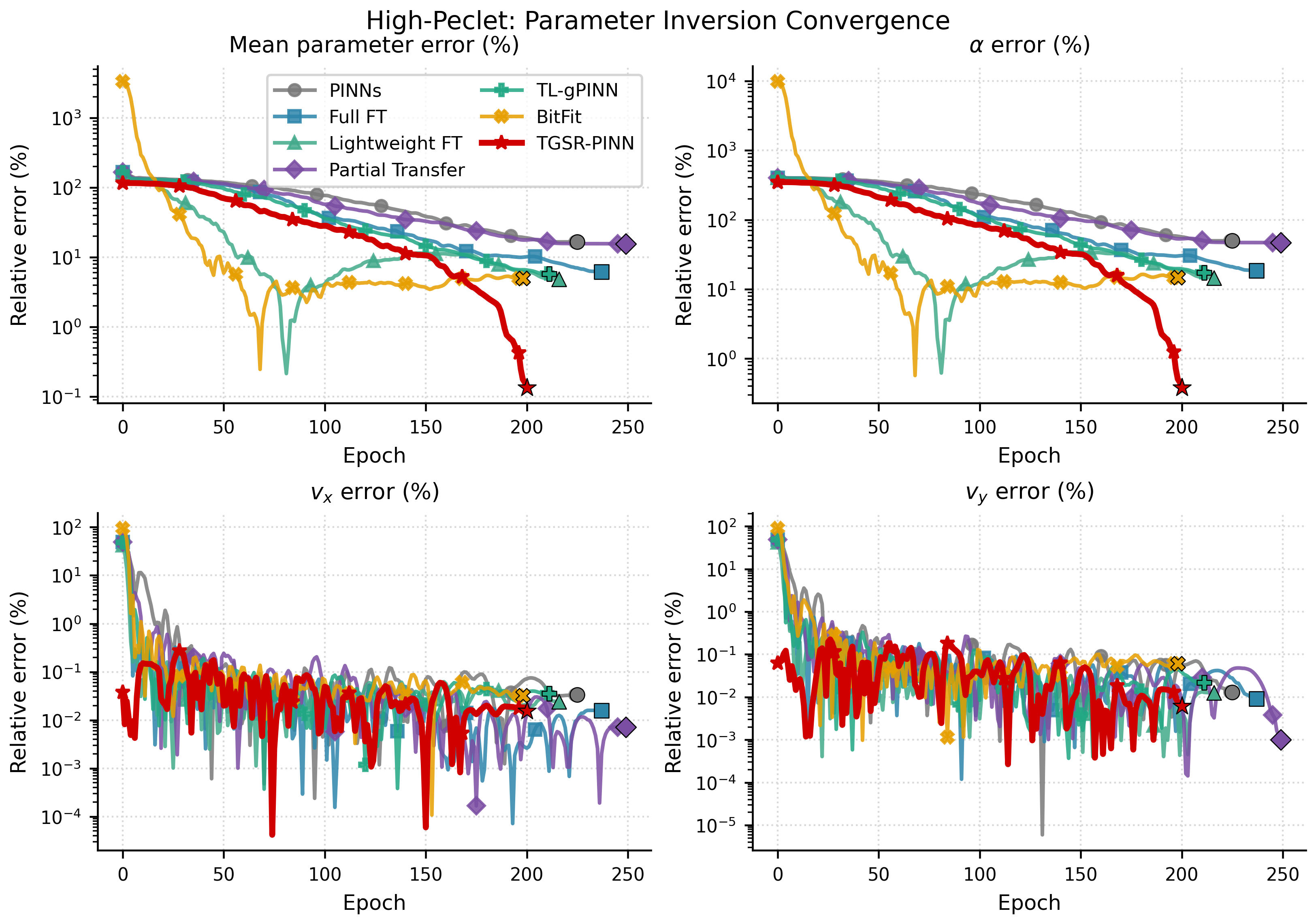
Figure 4 further shows that TGSR-PINN reduces the mean parameter error and the key diffusion-parameter error more consistently during the later training stage. The velocity parameters are recovered accurately by most methods, whereas the diffusion coefficient remains the main source of difficulty, confirming that the high-Péclet task mainly challenges parameter recovery rather than field reconstruction.
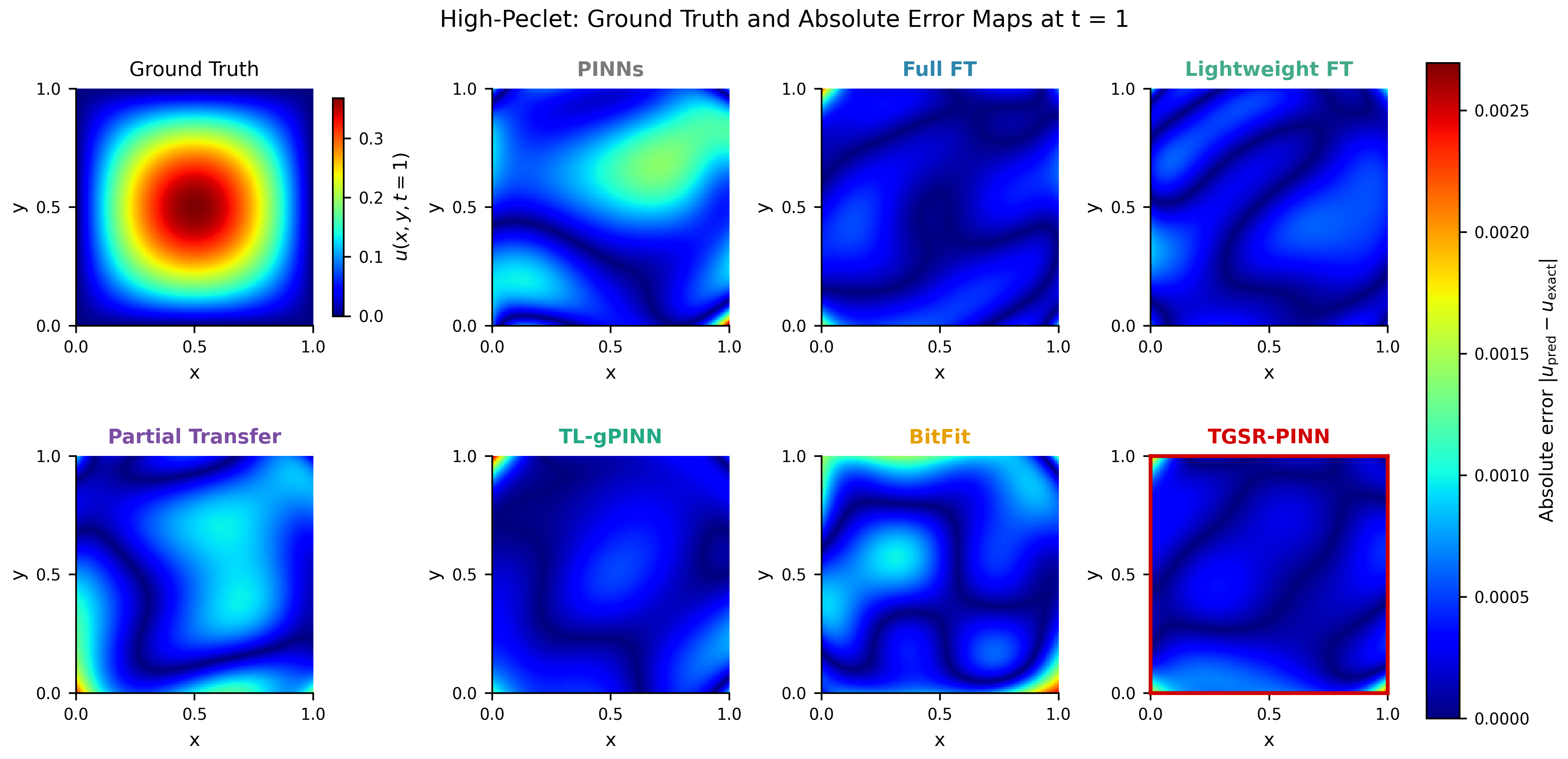
Figure 5 indicates that the absolute error of TGSR-PINN is more concentrated near low-error regions than those of the competing transfer baselines. This visual comparison is consistent with the quantitative results in Table 3, where TGSR-PINN achieves the lowest average field error and parameter error.
3.3 Cross-PDE-Family Transfer: Allen–Cahn \(\to\) Burgers Inverse Problem↩︎
The high-Péclet experiment primarily examines transfer from a 2D diffusion source task to a strongly advection-dominated target task. To further test whether the method remains effective when the dominant physical mechanisms differ between source and target, we construct an Allen–Cahn–Burgers cross-PDE-family transfer task. This task requires the model to transfer from a reaction–diffusion-dominated source model to a nonlinear advection and viscous diffusion target inverse problem, making it more likely to expose source representation bias and target parameter compensation issues.
The source task is a 1D Allen–Cahn inverse problem: \[u_{t} = \varepsilon^{2}u_{xx} + u - u^{3},\quad\text{infer }\varepsilon.\] The target task is a 1D Burgers inverse problem: \[u_{t} + uu_{x} = \nu u_{xx},\quad\text{infer }\nu.\] The Allen–Cahn source task uses \(\varepsilon=0.85\) as the initial value, \(\varepsilon=0.8\) as the true value, and 1% observation noise. The Burgers target task uses \(\nu=0.05\) as the initial value, \(\nu=0.01\) as the true value, and 3% observation noise. We use 11 random repetitions with LBFGS training and fixed-batch early stopping. BitFit is included as an additional parameter-efficient baseline to assess whether bias-only adaptation is sufficient under cross-PDE-family mechanism mismatch.
| Method | \(L_2\) error (%) | \(\nu\) error (%) | Time (s) |
|---|---|---|---|
| PINNs | \(0.300 \pm 0.080\) | \(0.781 \pm 0.755\) | 95 |
| Full FT | \(\mathbf{0.260 \pm 0.050}\) | \(0.568 \pm 0.399\) | 81 |
| Lightweight FT | \(0.800 \pm 0.440\) | \(12.565 \pm 27.800\) | 101 |
| Partial Transfer | \(0.290 \pm 0.060\) | \(0.832 \pm 0.621\) | 92 |
| BitFit | \(69.010 \pm 13.080\) | \(4891 \pm 13133\) | 87 |
| TGSR-PINN | \(0.268 \pm 0.058\) | \(\mathbf{0.408 \pm 0.260}\) | 92 |
Table 5 shows that TGSR-PINN and Full Fine-Tuning achieve the lowest relative \(L_2\) field errors at \((0.268\% \pm 0.058\%)\) and \((0.260\% \pm 0.050\%)\), respectively. The small field error difference demonstrates that relying solely on field reconstruction accuracy is insufficient to distinguish parameter recovery quality in cross-PDE transfer. In contrast, TGSR-PINN’s average \(\nu\) error of \((0.408\% \pm 0.260\%)\) is lower than Full Fine-Tuning’s \((0.568\% \pm 0.399\%)\), a relative reduction of approximately 28.2%. This indicates that neuron target scoring and selective soft decay can improve target physical parameter inversion while maintaining comparable field accuracy. Meanwhile, Lightweight FT and Partial Transfer show significantly increased parameter errors, suggesting that simply freezing partial layers or transferring only selected layers may struggle with deep representation mismatch in cross-PDE-family scenarios.
BitFit’s relative \(L_2\) field error in Table 5 is \((69.010\% \pm 13.080\%)\), significantly higher than other stable methods. All 11 BitFit repetitions produce finite final field and \(\nu\) errors; the repetition-level field error range is 47.78%–99.95% (median 69.16%), and the \(\nu\) error range is 13.88%–46355.98% (median 511.89%). Therefore, BitFit’s CrossPDE results should be interpreted as large-scale training instability or representation adaptation failure. This also indicates that while bias-only updates can be competitive in high-Péclet tasks, in cross-PDE-family transfer with stronger dominant mechanism differences such as Allen–Cahn to Burgers, bias degrees of freedom are insufficient to stably reconstruct the representations required by the target equation.
Figure 6 presents the repetition-level distribution of final \(\nu\) relative errors across 11 random repetitions. Each scatter point corresponds to one repetition; boxes indicate interquartile ranges, and values in the figure are medians. Due to BitFit’s extremely large \(\nu\) errors in some repetitions, the vertical axis uses a logarithmic scale. Together with Table 5, this figure shows that TGSR-PINN’s \(\nu\) errors are more concentrated in the low-error interval, indicating more stable parameter recovery in cross-PDE-family transfer.
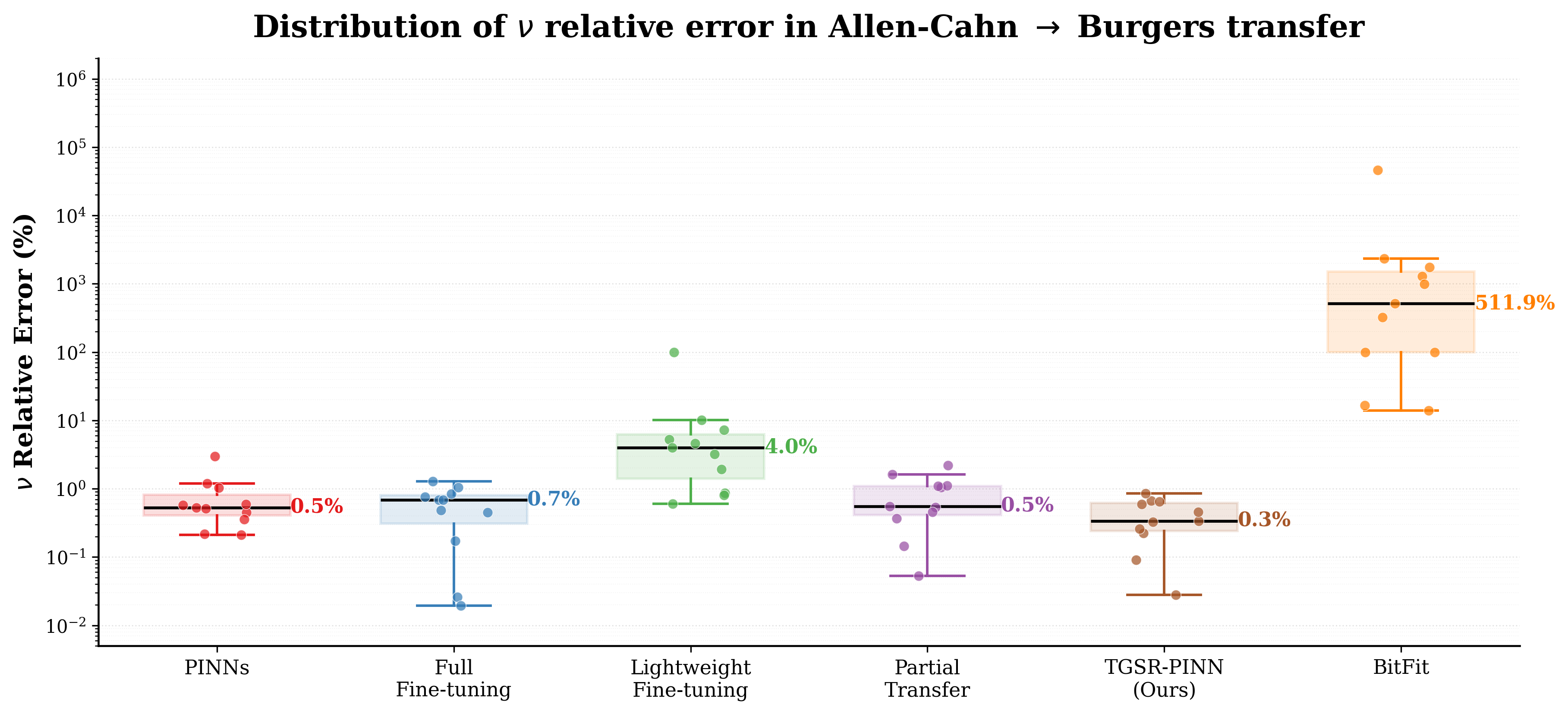
Figure 6 reveals that TGSR-PINN produces a more compact low-error distribution of the recovered viscosity parameter. In contrast, BitFit exhibits extremely large outliers, suggesting that bias-only adaptation is insufficient when the source and target PDEs have substantially different dominant mechanisms.
3.4 2D Reaction–Diffusion Inverse Problem: 5% Noise↩︎
Following the high-Péclet main experiment and cross-PDE-family transfer, we further examine a dual-parameter inverse problem with milder source–target differences but noisy observation data. The 2D reaction–diffusion target task is: \[\begin{align} u_{t} - \alpha(u_{xx} + u_{yy}) + \rho u^{2} &= Q_{T}(x,y,t),\\ \text{infer}\quad &\alpha,\rho. \end{align}\] This task transfers from a 2D diffusion source task to a target task with a reaction term, inferring diffusion coefficient \(\alpha\) and reaction coefficient \(\rho\). Compared to the high-Péclet task, the source–target difference is milder: both tasks are based on diffusion-type dynamics, but the target task additionally includes a nonlinear reaction term, and 5% noise is added to the target observation data only (not to PDE collocation, initial condition, or boundary condition points). Table 6 reports the mean and standard deviation over 7 random repetitions, presenting them in separate columns. Since the source–target difference is mild and the performance improvement is smaller than in the high-Péclet and cross-PDE-family main experiments, we position this as a noisy dual-parameter auxiliary case.
| Method | \(L_2\) mean (%) | \(L_2\) std (%) | Param mean (%) | Param std (%) | Time (s) |
|---|---|---|---|---|---|
| PINNs | 0.229 | 0.021 | 1.151 | 1.393 | 192 |
| Full FT | 0.228 | 0.033 | 1.378 | 1.341 | 155 |
| Lightweight | 0.238 | 0.030 | 1.329 | 0.849 | 104 |
| Partial | 0.237 | 0.035 | 1.606 | 1.621 | 176 |
| TL-gPINN | 0.231 | 0.034 | 1.308 | 1.589 | 378 |
| TGSR-PINN | 0.219 | 0.026 | 1.042 | 1.311 | 194 |
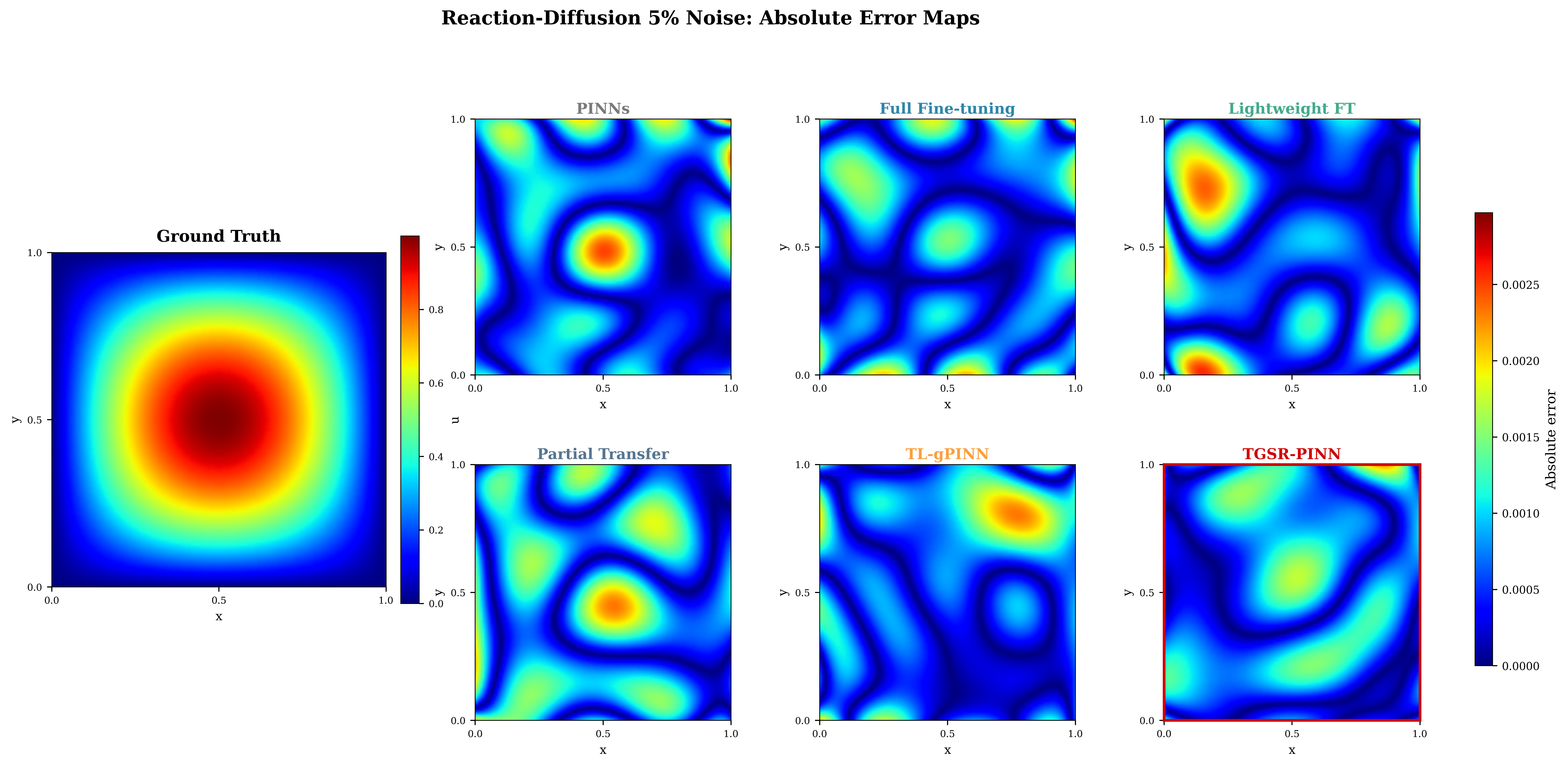
Table 6 shows that TGSR-PINN achieves the lowest average field error and average parameter error in this 5%-noise setting, but the field error gap relative to the best non-TGSR baseline is small, and the parameter error standard deviation is relatively large. Since average parameter error is a non-negative absolute relative error, Table 6 reports mean and standard deviation in separate columns to avoid misinterpreting the standard deviation as an error range. This result should therefore be interpreted as supplementary evidence in a noisy dual-parameter scenario rather than as the primary basis for the method’s robustness claim. Figure 7 presents the absolute error maps for the 5%-noise reaction–diffusion task under the same conditions.
Figure 7 shows that the general reaction–diffusion field structure can be reconstructed under 5% observation noise, while TGSR-PINN produces a relatively lower absolute error pattern. This supports the quantitative observation in Table 6 that the improvement in this milder noisy setting is positive but less pronounced than in the high-Péclet and cross-PDE transfer cases.
3.5 High-Péclet Mechanism Ablation, Scoring Batch Count, and Layer-Wise Diagnosis↩︎
These ablation experiments adopt the same high-Péclet task settings as Section 3.2. Considering that different ablation experiments vary in computational purpose and repetition count, we distinguish their interpretation levels by evidence function and avoid direct mixing with the main experiment results in Table 3. The first category comprises early mechanism observations and stress tests, including target short adaptation/random reset comparison, scoring batch count, data sparsity, and target short adaptation length analysis, primarily used to assess whether components exhibit reasonable trends. The second category consists of paired mechanism diagnoses. The core counterfactual, layer-protection, and selective soft decay mapping ablations use 10 paired repetitions with the same source model, target data settings, and training budget. These paired comparisons provide the main ablation evidence reported in this section. Other diagnostics, including the GMM/rank fallback check and the \(\alpha_s\) scoring-component sweep, are treated as sensitivity or mechanism observations rather than primary evidence for performance gain.
3.5.1 Mechanism ablation: target short adaptation, random reset, and selective soft decay↩︎
In the mechanism ablation experiment, we compare three settings: Target-Adaptation Only (only target short adaptation, no neuron target scoring or subsequent parameter reorganization), Random Reset (retains neuron target scoring and weak-adaptation signal estimation but replaces selective soft decay with random initialization-style resetting), and TGSR-PINN (complete method).
| Method | \(L_2\) error (%) | Param error (%) |
|---|---|---|
| Target-Adaptation Only | \(0.144 \pm 0.010\) | \(19.577 \pm 1.689\) |
| Random Reset | \(0.168 \pm 0.009\) | \(19.457 \pm 0.979\) |
| TGSR-PINN | \(\mathbf{0.069 \pm 0.006}\) | \(\mathbf{2.555 \pm 2.024}\) |
Table 7 shows that while Target-Adaptation Only exposes the transferred model to the target loss, the average parameter error remains at 19.577%, indicating that target short adaptation alone is insufficient to eliminate the adverse effects of source-side representations. Random Reset’s parameter error of 19.457% is close to Target-Adaptation Only, suggesting that even when low-scoring neurons are located, random initialization-style resetting may destroy partially reusable representations and introduce additional optimization perturbation. In contrast, the full TGSR-PINN reduces the average parameter error to 2.555% while lowering the relative \(L_2\) field error to 0.069%. This early diagnostic result indicates that neither target short adaptation nor random resetting can explain the full TGSR-PINN benefit. The subsequent paired ablations further examine specific components including neuron target scoring, neuron correspondence, layer protection, and selective soft decay mapping.
To further test whether the full method’s benefit comes from neuron target scoring and neuron correspondence rather than general weight perturbation, we run paired counterfactual ablations over 10 paired repetitions under the same source model, target task, noise level, target data settings, and optimization budget. Results are shown in Table 8.
| Method | \(n\) | \(L_2\) (%) | Param (%) | \(\alpha\) (%) | Wilcoxon |
|---|---|---|---|---|---|
| TGSR-PINN | 10 | \(\mathbf{0.074\pm0.015}\) | \(\mathbf{3.782\pm3.068}\) | \(\mathbf{11.312\pm9.205}\) | — |
| Random Soft Decay | 10 | \(0.084\pm0.012\) | \(5.216\pm2.377\) | \(15.613\pm7.122\) | \(p=0.037\) |
| Score-Shuffled | 10 | \(0.084\pm0.023\) | \(5.907\pm3.574\) | \(17.688\pm10.727\) | \(p=0.014\) |
Table 8 shows that TGSR-PINN’s average parameter error is 3.782% \(\pm\) 3.068%, lower than Random Soft Decay’s 5.216% \(\pm\) 2.377% and Score-Shuffled TGSR’s 5.907% \(\pm\) 3.574%. In the paired repetition comparison, TGSR-PINN is better in 8/10 pairs in both comparisons; the median paired parameter-error increases of the two counterfactuals are \(+1.065\) percentage points and \(+2.278\) percentage points, with two-sided Wilcoxon \(p=0.037\) and \(p=0.014\), respectively. These results indicate that the benefit cannot be attributed to arbitrary soft perturbation alone: target-informed neuron selection and preserving the score–neuron correspondence are both important.
3.5.2 Scoring batch count ablation↩︎
This subsection presents early diagnostic results on scoring batch count and data sparsity, examining the sensitivity of neuron target scoring to variations in sampling batches and observation data volume. These results serve as mechanism observation and stress testing; the main robustness evidence comes from multi-repetition experiments.
| \(K\) | \(L_2\) error (%) | Param error (%) |
|---|---|---|
| 1 | 0.0693 | 2.662 |
| 3 | 0.0693 | 2.555 |
Table 9 shows that increasing the scoring batch count from \(K=1\) to \(K=3\) leaves the \(L_2\) error essentially unchanged while the parameter error decreases slightly from 2.662% to 2.555%. This indicates that multi-batch scoring helps reduce single-batch randomness, yielding a modest improvement under the current protocol.
| Method | \(N_d=1000\) | \(N_d=50\) |
|---|---|---|
| PINNs | 19.1% / 0.09% | 30.6% / 0.12% |
| Full FT | 19.7% / 0.10% | 16.8% / 0.11% |
| TGSR-PINN | 2.3% / 0.09% | 11.4% / 0.10% |
Table 10 presents a single-run data sparsity stress test. When the observation count drops from \(N_d=1000\) to \(N_d=50\), TGSR-PINN’s \(\alpha\) error increases from 2.3% to 11.4%, indicating that extreme sparsity weakens parameter recovery; however, compared to PINNs (30.6%) and Full FT (16.8%), TGSR-PINN still maintains lower error in this stress test.
| \(E_{ad}\) | Rep A \(\alpha\) error | Rep B \(\alpha\) error | Fraction of main |
|---|---|---|---|
| 10 | 14.6% | 12.5% | 6.7% |
| 20 | 15.7% | 6.3% | 13.3% |
| 30 (default) | 9.2% | 6.2% | 20% |
| 60 | 11.4% | 6.9% | 40% |
Table 11 presents a preliminary sensitivity analysis of target short-adaptation length over 2 random repetitions. \(E_{ad}=30\) (20% of main training) achieves the lowest or comparable \(\alpha\) errors in both repetitions, and is therefore adopted as the fixed default setting for subsequent diagnostic experiments. This result indicates that adaptation length affects parameter recovery and provides empirical justification for the default setting; finer task-adaptive step selection is left for future work.
3.5.3 Scoring component ablation: \(\alpha_s\) parameter sweep↩︎
To address the question “why Taylor sensitivity and pre-activation variance must be used jointly,” we ablate the scoring components on the high-Péclet task. We sweep \(\alpha_s\) from 0 to 1 (step 0.1), with 5 random repetitions per setting.
| \(\alpha_s\) | \(\alpha\) mean | Best | Worst | All-param mean |
|---|---|---|---|---|
| 0.0 | 17.9% | 1.6% | 34.4% | 6.0% |
| 0.1 | 14.4% | 5.3% | 30.3% | 4.8% |
| 0.2 | 29.2% | 3.2% | 78.2% | 9.7% |
| 0.3 | 15.9% | 0.4% | 40.7% | 5.3% |
| 0.4 | 17.4% | 2.4% | 29.1% | 5.8% |
| 0.5 (default) | 13.8% | 2.3% | 38.1% | 4.6% |
| 0.6 | 16.2% | 1.3% | 28.0% | 5.4% |
| 0.7 | 15.2% | 7.8% | 35.7% | 5.1% |
| 0.8 | 13.2% | 1.6% | 38.5% | 4.4% |
| 0.9 | 18.1% | 8.3% | 40.5% | 6.1% |
| 1.0 | 14.6% | 1.9% | 33.3% | 4.9% |
The \(\alpha_s = 0.5\) (joint default) setting achieves a mean \(\alpha\) error of 13.8%, falling within the low-error plateau from 0.3 to 0.8; both endpoints perform systematically worse. The \(\alpha_s \in [0.3, 0.8]\) range forms a stable low-error plateau, with the default \(\alpha_s=0.5\) located in its center. Although \(\alpha_s = 0.8\) yields a slightly lower mean (13.2%) in this 5-repetition sweep, the difference is within one standard deviation. Combined with the 7-repetition main experiment results for \(\alpha_s = 0.5\) (mean \(\alpha\) error 13.25%, best 0.38%), we adopt \(\alpha_s=0.5\) as the fixed default. Figure 8 shows the complete \(\alpha_s\) sweep curve.
![Figure 8: \alpha_s parameter sweep curve. The \alpha_s \in[0.3, 0.8] range forms a low-error plateau, with higher errors at both ends.](/article/2607.05271/fig7.png "fig:")
3.5.4 GMM and rank fallback ablation↩︎
TGSR-PINN employs a dual-path design with GMM distribution diagnosis and rank fallback for weak-adaptation signal estimation. The core idea is: when the intra-layer neuron target score distribution exhibits a clear separation between low-scoring and high-scoring neuron clusters, the GMM branch exploits distributional information for finer weak-adaptation signals; when the distribution is relatively uniform or two-component evidence is insufficient, rank fallback provides a stable conservative alternative.
| Method | \(n\) | \(L_2\) (%) | Param (%) | \(\alpha\) (%) | Wilcoxon |
|---|---|---|---|---|---|
| TGSR (GMM+rank) | 5 | \(0.071\pm0.007\) | \(2.944\pm2.348\) | \(8.805\pm7.044\) | — |
| TGSR (rank only) | 5 | \(0.069\pm0.007\) | \(3.090\pm2.380\) | \(9.239\pm7.140\) | \(p=0.593\) |
Table 13 shows that the rank-only version produces field and parameter errors very close to the full TGSR-PINN, with a Wilcoxon test \(p = 0.593\). In the current high-Péclet diagnostic task, most hidden layers’ neuron target score distributions do not exhibit strongly separated bimodal structure (the \(\Delta \mathrm{BIC}\) condition is not met), so the automatic switching mechanism activates the rank fallback path for most layers. Thus, rank fallback is the primary active route in this diagnostic setting, while retaining the GMM branch does not introduce additional perturbation or instability. We therefore do not treat the GMM branch as an independent source of the observed performance gain in this task; instead, its value lies in conditional enhancement—when the target task or network layer’s neuron target score distribution exhibits a clear low-scoring-neuron cluster, the GMM branch can activate and provide finer distributional diagnosis than ranking alone.
3.5.5 Layer protection ablation↩︎
| Method | \(n\) | \(L_2\) (%) | Param (%) | \(\alpha\) (%) | Avg. selective decay | Wilcoxon |
|---|---|---|---|---|---|---|
| Depth-aware (\(\beta_h\!=\!0.55\)) | 10 | \(0.074\pm0.015\) | \(3.782\pm3.068\) | \(11.312\pm9.205\) | \(0.044\pm0.011\) | — |
| No protection (\(\beta_h\!=\!0\)) | 10 | \(0.092\pm0.023\) | \(7.478\pm2.869\) | \(22.395\pm8.592\) | \(0.101\pm0.040\) | \(p\!=\!0.002\) |
TGSR-PINN controls the selective soft decay intensity at different depths through the layer protection coefficient \(\beta_h\). Intuitively, shallow layers are more likely to contain input encoding and low-order spatial structures and thus receive stronger protection; deeper layers are more likely to carry source-task-related local patterns and therefore allow more thorough correction. The overall intensity matching control first computes layer protection coefficients under the default \(\beta_h=0.55\), then takes a neuron-count-weighted average to obtain a uniform protection coefficient applied to all hidden layers with the same weak-adaptation signal scaling intensity.
Table 14 shows that after removing layer protection, the relative \(L_2\) field error increases from 0.074% to 0.092%, the average parameter error from 3.782% to 7.478%, and the \(\alpha\) error from 11.312% to 22.395%. Paired statistics further show that the no-protection version produces higher average parameter error on all 10/10 paired repetitions, with a median paired increase of \(+3.437\) percentage points and a two-sided Wilcoxon \(p=0.002\). This result shows that under this high-Péclet diagnostic protocol, completely removing shallow protection significantly increases selective soft decay intervention intensity and degrades parameter recovery.
An additional overall-intensity-matched diagnostic is used only as supplementary mechanism evidence. It suggests that controlling the total intervention intensity is an important stabilizing factor, whereas the extra contribution of depth-wise allocation is more modest and task-dependent.
The applicability boundary of layer protection is task-dependent. Under the high-Péclet diagnostic setting, shallow protection as an empirical stability constraint helps avoid additional perturbation from excessive selective soft decay. The supplementary overall-intensity-matched diagnostic indicates that total intervention intensity is a major stabilizing factor, while the extra effect of depth-wise allocation is modest and not used here as primary positive evidence. For scenarios with stronger source–target differences or severely misaligned target parameter initial values, layer protection strength can be further adapted in a task-specific manner.
3.5.6 Selective soft decay mapping form ablation↩︎
| Mapping | \(n\) | \(L_2\) (%) | Param (%) | \(\alpha\) (%) | Wilcoxon |
|---|---|---|---|---|---|
| Linear | 10 | \(0.095\pm0.017\) | \(7.051\pm3.795\) | \(21.106\pm11.380\) | \(p\!=\!0.002\) |
| Piecewise cubic (default) | 10 | \(\mathbf{0.074\pm0.015}\) | \(\mathbf{3.782\pm3.068}\) | \(\mathbf{11.312\pm9.205}\) | — |
| Sigmoid | 10 | \(0.092\pm0.021\) | \(7.361\pm3.358\) | \(22.040\pm10.077\) | \(p\!=\!0.004\) |
| Hard threshold | 10 | \(0.093\pm0.020\) | \(6.430\pm3.283\) | \(19.249\pm9.852\) | \(p\!=\!0.027\) |
Eq. (19 ) uses a piecewise cubic function to map weak-adaptation signals to continuous scaling coefficients. Table 15 shows that under this 10-repetition paired setting, the default piecewise cubic mapping achieves the lowest field error, average parameter error, and \(\alpha\) error. Relative to the default mapping, linear, sigmoid, and hard threshold mappings increase average parameter error by 3.269, 3.579, and 2.648 percentage points respectively, and \(\alpha\) error by 9.794, 10.728, and 7.937 percentage points respectively, with two-sided Wilcoxon \(p=0.002\), \(0.004\), and \(0.027\). The relatively small field error differences contrasted with pronounced parameter error differences indicate that the selective soft decay mapping form primarily affects subsequent parameter recovery rather than merely changing field reconstruction accuracy.
Synthesizing the ablation results in Section 3.5, TGSR-PINN’s weak-adaptation signal estimation and correction pipeline can be summarized as: target short adaptation provides the target-side diagnostic state \(\to\) neuron target scoring through Taylor sensitivity and pre-activation variance (\(\alpha_s=0.5\)) \(\to\) weak-adaptation signal estimation through GMM and rank fallback \(\to\) low-scoring neuron identification \(\to\) layer-protected selective soft decay (\(\beta_h=0.55\)) with a bounded decay mapping. These results support the following empirical interpretation: neuron target scoring provides target-side evidence, and the paired counterfactuals show that random soft decay and score shuffling are significantly worse than TGSR-PINN at \(n=10\); layer protection reduces the risk of shallow-layer over-correction, with no-protection variants significantly worse on all paired repetitions; and the default piecewise cubic mapping performs significantly better than linear, sigmoid, and hard-threshold mappings. In the current high-Péclet diagnostic setting, rank fallback provides the main stable route for weak-adaptation signal estimation, while the GMM branch remains a conditional distributional enhancement when clear low-scoring neuron clusters are present. Tables 7, 9, 10, and 11 primarily serve as early mechanism observations; Tables 8, 14, and 15 provide the main 10-repetition paired mechanism evidence.
4 Discussion↩︎
4.1 Joint Analysis of Field Error and Parameter Error↩︎
In PINN inverse problems, physical field errors and physical parameter errors are not always synchronized. The network may compensate for parameter bias by adjusting the field representation, achieving low field prediction errors while still failing to recover the correct target physical parameters. Therefore, this paper uses both relative \(L_2\) field error and parameter error as the basis for evaluating inverse transfer effectiveness, rather than judging transfer success solely by field reconstruction accuracy.
From the high-Péclet number 2D advection–diffusion and Allen–Cahn \(\to\) Burgers cross-PDE-family transfer results, TGSR-PINN’s primary value lies in improving target parameter recovery when field accuracy is comparable. In the high-Péclet task, the average parameter error gap between TGSR-PINN and Lightweight FT is limited, and the average \(\alpha\) error is still approximately 13.25%; thus the advantage in this task manifests as a comprehensive performance across physical field error, average parameter error, best \(\alpha\) recovery potential, and repetition-level diagnostics. At the same time, TGSR-PINN’s parameter error exhibits a relatively large standard deviation in the high-Péclet task, indicating sensitivity to random initialization, observation sampling, and optimization paths; this paper therefore reports mean, standard deviation, best repetition, and parameter-level errors simultaneously to more fully characterize parameter recovery stability. The Allen–Cahn \(\to\) Burgers task further indicates that when source and target dominant physical mechanisms differ but field errors are at the same magnitude, neuron target scoring and selective soft decay can still improve target physical parameter recovery. The 5%-noise reaction–diffusion experiment provides supplementary evidence in a noisy dual-parameter scenario under milder source–target differences, but its smaller performance gap and larger parameter-error variance should not be overinterpreted as the main robustness evidence.
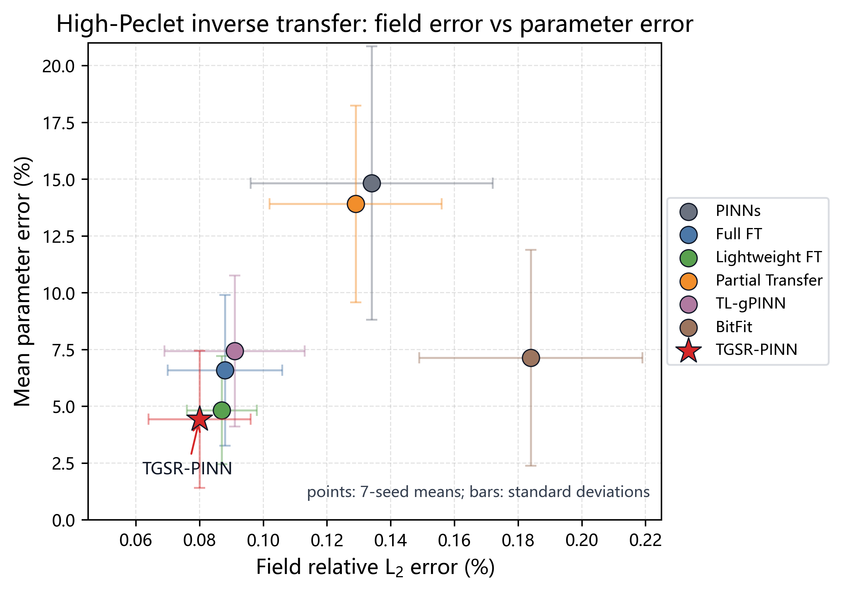
Figure 9, based on the 7-repetition aggregated results from Table 3, illustrates the potential decoupling between relative \(L_2\) field error and average parameter error in the high-Péclet experiment. Each point represents a method’s cross-repetition mean, with horizontal and vertical error bars indicating field error and parameter error standard deviations respectively. The figure highlights that several baselines obtain field errors close to TGSR-PINN, but their parameter errors remain substantially higher. Therefore, for inverse problems where parameter identification is the core objective, reporting only field error is insufficient; parameter-level error and repetition-level stability must be simultaneously analyzed.
4.2 Analysis of Selective Soft Decay↩︎
As described in Section 2.2, TGSR-PINN implements transfer representation correction through the pipeline of “target short adaptation \(\to\) neuron target scoring \(\to\) weak-adaptation signal estimation \(\to\) layer protection \(\to\) selective soft decay.” This section discusses why this pipeline may produce benefits and combines ablation results to illustrate the functional boundaries of different components.
The mechanism ablation results on the high-Péclet task support the role of selective soft decay. Target-Adaptation Only shows that merely exposing the transferred model briefly to the target loss is insufficient to stably improve parameter recovery; Random Reset shows that strong random resetting of low-scoring neurons may destroy partially reusable source representations and introduce additional optimization perturbation. In contrast, TGSR-PINN employs selective soft decay, reducing the influence of low-scoring neurons while preserving network topology and recoverability. Further 10-repetition paired counterfactual ablation shows that Random Soft Decay and shuffling the score–neuron correspondence significantly increase parameter error. These results indicate that the full method’s benefit cannot be simply attributed to general weight perturbation but more likely arises from the combined effect of target-informed neuron selection, score–neuron correspondence, layer protection, and selective soft decay.
From an optimization dynamics perspective, PINN inverse problems may exhibit compensatory states where “field prediction is acceptable but parameters are wrong.” When network representations and physical parameters are jointly optimized, certain transferred representations may make subsequent training more likely to enter such compensation regions. Selective soft decay modulates the pre-activation magnitude of low-scoring neurons, changing the initial state of the main training phase, thereby alleviating part of the parameter compensation caused by mismatched transferred representations.
Figure 10 shows the parameter-error convergence curves during target training, whereas Figure 11 compares the parameter errors before target short adaptation, after selective soft decay, and at the final training stage. Together, these two figures indicate that selective soft decay mainly influences the subsequent parameter recovery trajectory rather than acting as a simple field-error reduction trick.
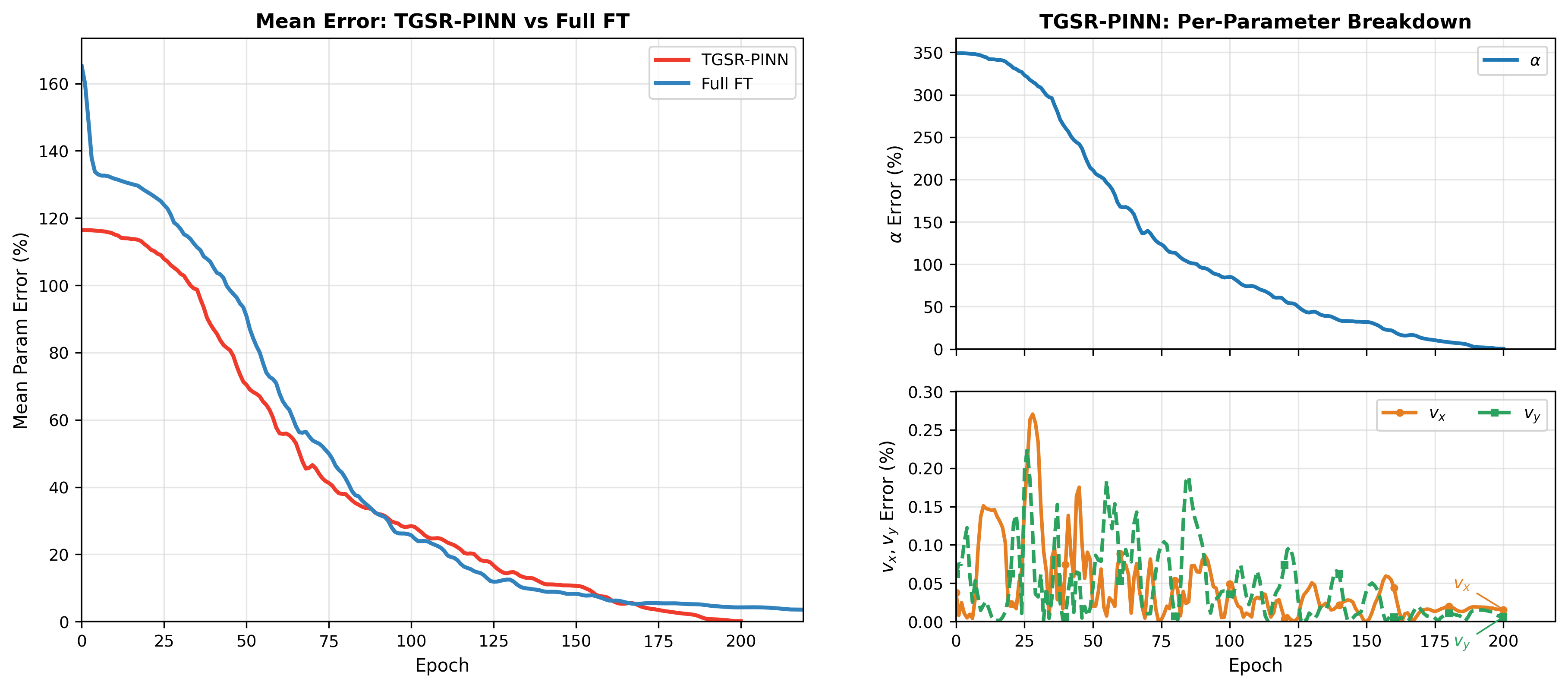
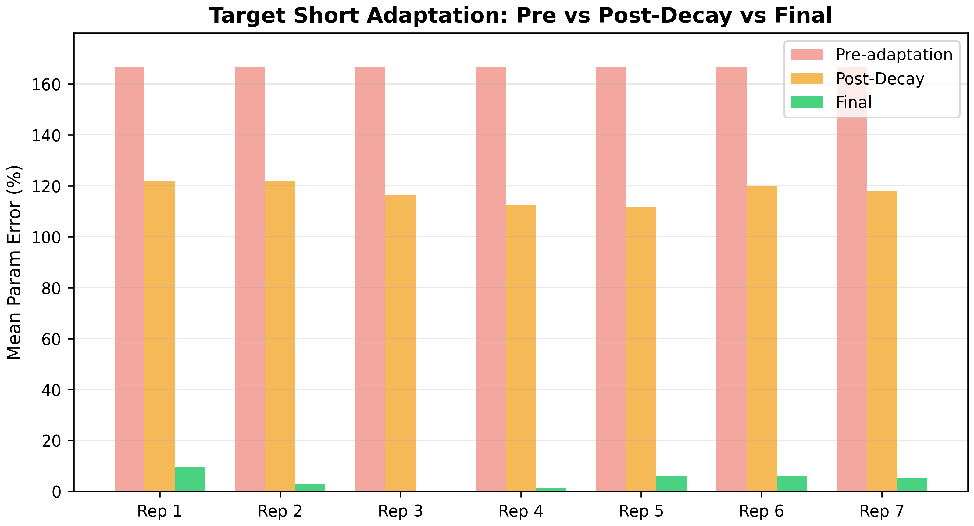
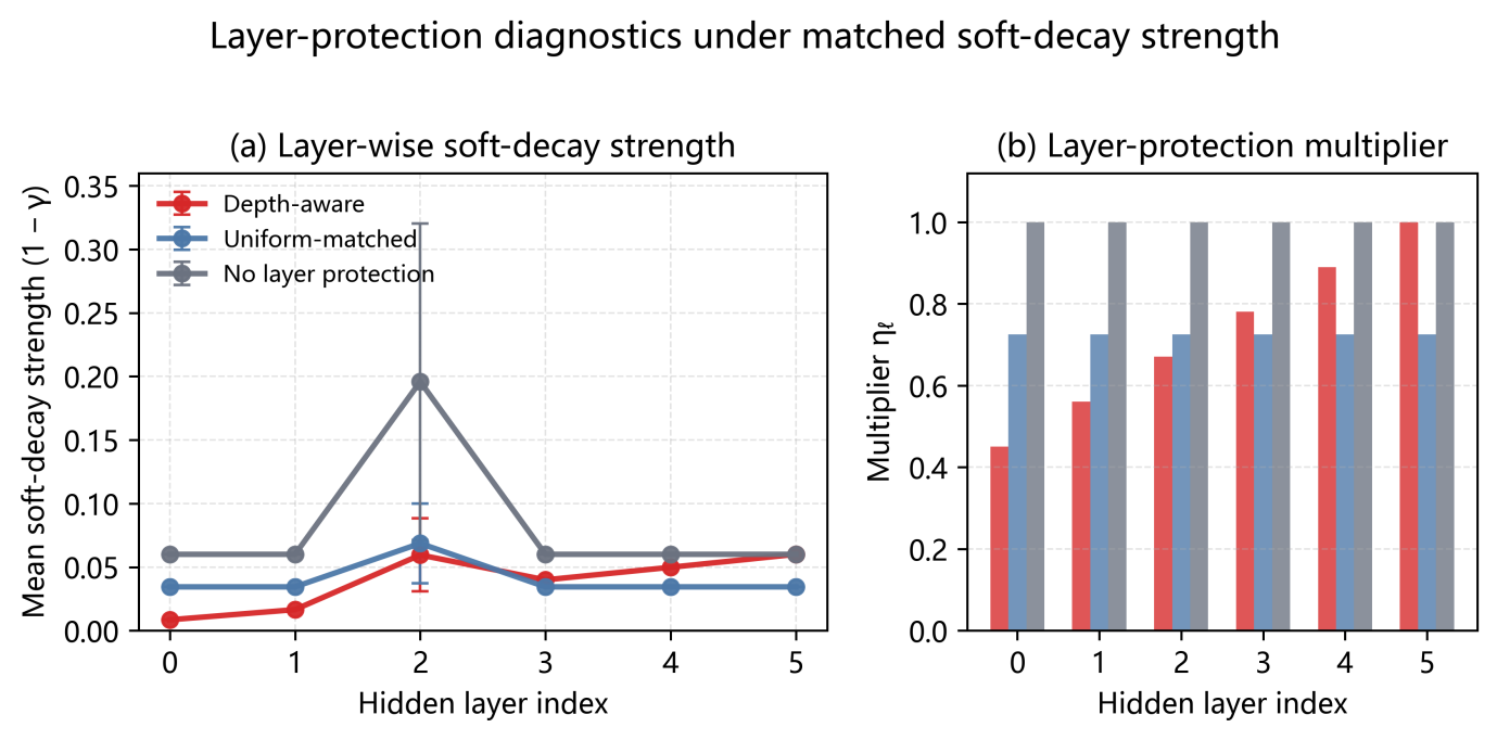
The design motivation for layer protection is: shallow representations of the source model may contain more general input encoding and low-order spatial structures, while deeper representations are more likely to carry source-task-related local patterns. Therefore, when TGSR-PINN performs selective soft decay, it applies weaker intervention to shallow layers and allows stronger correction for deeper layers. Figure 12 further provides layer-wise diagnostic results for the layer protection ablation: Figure 12 (a) compares the layer-wise average selective soft decay intensity under default depth-aware protection, overall intensity matching, and no protection; Figure 12 (b) shows the corresponding layer protection coefficients. This result is consistent with Table 14, showing that removing layer protection significantly increases selective soft decay intensity and degrades parameter recovery. The overall intensity matching control is treated as supplementary context: it helps distinguish the effect of total intervention strength from the weaker and task-dependent effect of depth-dependent allocation.
TGSR-PINN differs from traditional pruning methods in its objective. Traditional pruning typically serves model compression and inference acceleration, while TGSR-PINN targets representation adaptation in PINN inverse transfer. Selective soft decay does not delete neurons or randomly reset them, but rather reduces the influence of low-scoring neurons on target optimization through continuous decay, improving target-side parameter recovery while retaining reusable source knowledge. The weak-adaptation signal in this paper serves as the continuous basis for selective soft decay, characterizing the low-scoring neurons under the current target loss and target sample response.
4.3 Computational Overhead and Applicability Boundaries↩︎
| Component | Time (s) | Memory (MB) | Notes |
|---|---|---|---|
| Target short adaptation | \(\sim\)45 | \(\sim\)234 | 20% of main training |
| Neuron scoring | \(\sim\)3 | \(\sim\)470 | Forward+backward |
| GMM + selective soft decay | \(\sim\)2 | \(<\)1 | 1D distribution |
| Total | \(\sim\)50 | \(\sim\)470 | 13–19% of Full FT |
TGSR-PINN introduces three additional steps on top of Full Fine-Tuning: target short adaptation, neuron target scoring, and selective soft decay. Table 16 provides the time and memory overhead for each step. The overhead statistics are based on the same network width and sampling batch settings as the high-Péclet main experiment (PDE 10000, BC 2500, IC 2500, data 1000), on a Windows 11 workstation with AMD Ryzen 5 9600X CPU and NVIDIA GeForce RTX 5070 GPU (12 GB), using Python 3.13.7, PyTorch 2.11.0.dev20260127+cu128, and CUDA 12.8. The reported times cover only the training process and TGSR-PINN additional steps, excluding offline data generation, plotting, final dense-grid evaluation, and result aggregation; these post-processing steps are identical across all methods and are therefore not counted as additional method overhead.
All methods use the same batch size settings and the same LBFGS implementation. Each LBFGS outer epoch uses max_iter=20 and history_size=100, with a fixed training batch per LBFGS stage to maintain stable closure evaluation.
Training early stopping is triggered only by training loss improvement: 10 consecutive rounds without sufficient improvement or adjacent loss change below \(10^{-8}\), without using test field error or true physical
parameter error. Since different repetitions may trigger different early stopping rounds, the times in Table 16 should be understood as empirical overhead from representative runs rather than hardware-independent complexity
conclusions; complete reproduction materials retain per-repetition runtime and early stopping information. In the high-Péclet 2D task, TGSR-PINN’s total training time is 266s (Full FT: 235s), with approximately 13% overhead. It is worth noting that the
main training stage of TGSR-PINN is slightly faster than Full FT in this representative run, but this observation should not be interpreted as a general acceleration guarantee across tasks. The cross-PDE task’s overhead proportion is slightly higher (19%),
mainly because 1D problems have shorter main training times, making the target short adaptation relatively larger. Therefore, TGSR-PINN’s additional overhead should be understood as the cost of trading limited training time for parameter recovery
stability, not as a training acceleration strategy.
GMM fitting performs two-component EM estimation on the 1D neuron target score distribution of 100 neurons per layer, with computational complexity independent of the problem’s spatial dimensionality (1D/2D/3D). Under the network scale used in this paper, GMM fitting and selective soft decay consume far less time than target short adaptation and neuron target scoring; therefore, TGSR-PINN’s main computational cost comes from target short adaptation, which can be further compressed by adjusting the adaptation proportion (\(E_{ad}\)). GMM fitting, as a low-overhead distributional diagnosis step following neuron target scoring, provides intra-layer distributional information for weak-adaptation signal estimation.
In terms of applicability boundaries, TGSR-PINN is more suitable for inverse transfer scenarios where source and target share partially reusable representations, but direct transfer may introduce parameter recovery bias. The method’s effectiveness depends on the target short adaptation phase providing reasonably reliable target evidence. When the initial target physical parameters deviate severely from true values, or short adaptation has already entered an incorrect parameter compensation region, neuron target scores and weak-adaptation signals may be contaminated, leading to insufficient parameter updates or parameter locking. Layer protection, GMM/rank fallback estimation, and piecewise cubic selective soft decay have demonstrated empirical effectiveness as a combined pipeline under the current experimental settings; their task-adaptive generalization is one direction for future research. Furthermore, the experiments in this paper are all based on benchmark inverse problem settings with known true values, facilitating parameter error and repetition-level stability assessment; model error, observation bias, unknown boundary conditions, and measurement noise in real engineering data still require dedicated future validation. Adaptive selection of the bounds for selective soft decay (\(\gamma_m\) and \(\gamma_{\min}\)) is also left as future work.
5 Conclusion↩︎
This paper proposes TGSR-PINN, a target-evidence-driven neuron-level representation adaptation method for PINN inverse transfer learning. The method does not transfer source-task physical parameters; instead, after target short adaptation, it computes neuron target scores using Taylor sensitivity and pre-activation variance, estimates weak-adaptation signals through a GMM and rank fallback dual-path mechanism, and applies selective soft decay to low-scoring neurons. Compared with full fine-tuning, frozen-layer transfer, or partial-layer transfer, TGSR-PINN focuses more on the empirical adaptation evidence of transferred hidden representations in target inverse problems and reduces the influence of low-scoring neurons on subsequent target optimization through gentle continuous reweighting.
Experimental results show that TGSR-PINN presents empirical advantages in the examined inverse transfer scenarios with significant source–target differences and strong parameter coupling. In the high-Péclet number 2D advection–diffusion task, TGSR-PINN achieves the lowest average field error and average parameter error, and shows the best \(\alpha\) parameter recovery potential; this result indicates that target-side representation correction can benefit parameter recovery in challenging advection-dominated inverse problems. In the Allen–Cahn \(\to\) Burgers cross-PDE-family transfer, TGSR-PINN achieves lower \(\nu\) parameter error while maintaining field error comparable to Full Fine-Tuning, indicating that target-side representation correction provides benefits for parameter recovery. The 5%-noise reaction–diffusion experiment serves as supplementary validation in a noisy dual-parameter scenario, where the advantage is smaller and should be interpreted as supporting rather than primary evidence.
Mechanism ablation and counterfactual ablation show that target short adaptation alone or random resetting is insufficient to replace the full TGSR-PINN; Random Soft Decay and score shuffling are significantly worse than TGSR-PINN in the 10-repetition paired counterfactual comparison. The scoring component sweep shows that the joint scoring of Taylor sensitivity and pre-activation variance forms a relatively stable low-error plateau in the intermediate weight range; the GMM and rank fallback ablation indicates that rank fallback is the main active path in the current high-Péclet diagnostic setting, while GMM provides conditional distributional enhancement when clear low-scoring neuron clusters exist; the layer protection ablation shows that removing shallow protection significantly degrades parameter recovery; and the selective soft decay mapping ablation suggests that gentle continuous mapping helps reduce perturbation from excessive intervention.
Overall, TGSR-PINN transforms coarse-grained weight reuse in PINN inverse transfer into a target-evidence-driven neuron-level representation diagnosis and soft correction process. The framework’s main contribution lies in reassessing hidden representations using target-side evidence after transfer and reducing the influence of low-scoring neurons on target optimization through selective soft decay. Future work may address real engineering inverse problem validation, adaptive target adaptation step count, selective soft decay bound selection, parameter update sufficiency detection, dynamic loss weighting, explicit gating versus weight scaling comparison, multi-source transfer, and integration with neural operator methods to enhance TGSR-PINN’s applicability and scalability in more complex engineering inverse problems.
Code Availability↩︎
The source code, configuration files, and scripts for reproducing the experiments in this paper are publicly available at https://github.com/jooycelee/TGSR-Pinns. The repository includes the TGSR-PINN implementation, benchmark task configurations, and post-processing utilities used to generate the reported tables and figures.
Acknowledgements↩︎
This work is supported by the Foundation of Fujian Provincial Department of Education, China (Grant No. JAT251084 and JAT251087). The authors also thank the anonymous reviewers for their constructive comments that helped improve this paper.