Is the Geometry Doing the Work?
An Operating-Point Audit of Hierarchy in Hyperbolic Vision–Language Models
January 01, 1970
Abstract
Whether a hyperbolic representation model uses its geometry cannot be read off its curvature parameter. What matters is the dimensionless operating point \(\sqrt{c}\rho\) at which its embeddings sit, and whether the radial and cone machinery is active there. We develop a battery of necessary-condition diagnostics and apply it to three published hyperbolic vision–language families—MERU, HyCoCLIP, and PHyCLIP—across released checkpoints and controlled interventions on a fixed current-GRIT snapshot. The audit identifies three failure modes. First, curvature is not an active resource in any audited configuration. The operating point stays near-Euclidean (\(H(u)\approx1\); no evaluated converged checkpoint reaches \(\sqrt{c}\rho>1\)). Releasing the curvature floor moves scalar curvature and norms but keeps the operating point near-Euclidean, with no substantial downstream degradation across seeds. Second, the cone and traversal machinery is measured inoperative. Entailment cones are inactive, saturated, or misaligned, and graded traversal fails under controlled readouts across all families. Directed radial depth is a bounded non-detection: external parent–child norm ordering shows no signal above shuffle-null controls at quantified sensitivity. The only surviving signal, a small directed residual on the models’ native box\(\to\)caption relation, remains non-operative. Third, hierarchy-looking evaluations are underdetermined. Taxonomy correlations are carried by angular distance, and coarse-retrieval gains track box/compositional supervision, not curvature. A mechanistic account explains why: the entailment objective admits a low-curvature, wide-cone shortcut. A parameter-free aperture identity (cones saturate exactly when \(\sqrt{c}\rho\le2K\)) locates the edge at which every entailment-trained unclamped run—across families and seeds—settles. Entailment-off runs show no arrest there and are still contracting at every probed horizon. The shortcut is thus the dominant accelerator of collapse rather than its sole cause: contrastive/alignment training alone also fails to hold curvature high. We conclude that these formulations, as released, do not instantiate the radial/cone mechanism their geometry motivates. We distill the battery into a five-number geometry report that future hierarchy claims can adopt.
1 Introduction↩︎
Vision-language models are increasingly expected to reason not only about visual similarity, but also about abstraction: an image of a “golden retriever” is also an image of a “dog”, an “animal”, and an “entity”. This has motivated a growing line of hyperbolic vision-language models, including MERU [1], HyCoCLIP [2], and PHyCLIP [3], which replace Euclidean CLIP-style representations [4] with negatively curved spaces. The motivation is compelling: hyperbolic spaces have exponential volume growth and are known to embed tree-like structures with low distortion [5]–[8]. In this view, general concepts should lie closer to the origin, specific concepts should move toward the boundary, and entailment cones should encode asymmetric abstraction relations.
But do current hyperbolic vision-language models actually instantiate this hierarchy mechanism?
This question is more subtle than asking whether hyperbolic VLMs perform well on standard downstream benchmarks. A model can improve retrieval or classification through better contrastive alignment, compositional supervision, calibration, or regularization, without using nonlocal hyperbolic geometry. Conversely, a model can exhibit taxonomy-like semantic similarity in its angular structure without encoding directed radial hierarchy. Existing evaluations often conflate these possibilities: leaf-level classification does not test abstraction, symmetric taxonomy-distance correlations do not distinguish angular similarity from radial depth, and zero entailment violation can arise from saturated cones rather than learned hierarchy.
We therefore conduct a structural audit of public and from-scratch hyperbolic VLMs. Our study covers three representative model families—MERU, HyCoCLIP, and PHyCLIP—including seven released checkpoints and matched current-GRIT interventions. We separate two forms of evidence. First, we analyze released checkpoints as fixed artifacts, asking whether the public models exhibit the geometry and hierarchy mechanisms claimed for them. Second, because GRIT is a URL-derived corpus whose accessible subset changes over time, we train matched baselines and interventions on a fixed current-GRIT snapshot; all causal comparisons are made only within this current snapshot.
Our findings are fourfold. First, curvature is not a separately identifiable or performance-critical degree of freedom: across families and floor settings the operating point stays near-Euclidean (\(\sqrt{c}\rho\approx0.2\)–\(0.3\)), and unclamping the curvature floor changes the parameterization—\(c\) and the norms—but not the operational geometry, while downstream metrics show no substantial degradation (Section 4). Second, the cone and traversal machinery is measured inoperative—apertures saturated or misaligned, graded traversal failing under controlled readouts—while directed radial depth is a bounded non-detection: external parent–child ordering shows no signal above shuffle-null controls at quantified sensitivity (Section 5). Third, a gradient-level mechanism explains why natural interventions fail to install hierarchy: the entailment objective admits a low-curvature shortcut that widens cone apertures and suppresses violations without learning order. On the probed trajectories the entailment gradient pushes curvature down at every collapse-phase step (three seeds, both gradient-probed families), outweighing the contrastive gradient and any added depth signal. Removing the entailment term does not restore curvature—contrastive/alignment training alone also fails to hold it up—so the shortcut is the dominant accelerator of collapse rather than its sole cause (Section 7). Fourth, the evaluations usually read as evidence of hierarchy are underdetermined: the stronger taxonomy-distance correlation of hyperbolic checkpoints is carried by angular distance, and raw directed norm-ordering scores are confounded by marginal prompt statistics unless shuffle-controlled, so prior positive evidence should not be read as active radial or cone-based hierarchy without direct geometry diagnostics.
These results do not imply that hyperbolic geometry is useless for vision-language learning. They show that the current evidence for active hyperbolic hierarchy in published formulations is insufficient.
Our contribution is not a new hyperbolic VLM. Instead, we provide a diagnostic framework and a mechanistic explanation for why published formulations fail to activate the hierarchy mechanism their geometry motivates. Our contributions are fivefold:
We show that MERU, HyCoCLIP, and PHyCLIP checkpoints operate in a near-Euclidean regime, and that releasing the curvature floor preserves or lowers the image-side dimensionless radius \(\sqrt{c}\rho\).
We show that standard downstream metrics are decoupled from the entailment/order mechanism: curvature can collapse, cone constraints can saturate, and norm ordering can disappear while retrieval, compositionality, and zero-shot metrics remain comparable under matched comparison.
We give a mechanistic explanation for curvature collapse: the entailment objective admits a low-curvature shortcut—reducing curvature widens cone apertures and suppresses violations without learning order. A per-loss gradient decomposition (in the two gradient-probed families) shows the entailment term drives curvature down more strongly than any added depth signal can counteract. An entailment-off ablation shows this shortcut is the dominant accelerator rather than a necessary cause, since contrastive/alignment training alone also fails to hold curvature up (Section 7).
We provide direct hierarchy diagnostics—radial parent-child ordering, cone activity, traversal robustness, taxonomy angular/radial decomposition, and shuffle-controlled directed tests—and, aside from one small, non-operative exception (Section 5.1), find no evidence that the published formulations instantiate the active nonlocal hyperbolic hierarchy.
We identify design requirements for hyperbolic VLMs: curvature-identifying supervision, controlled radial representation learning, entailment objectives that do not reward low-curvature wide-cone shortcuts, and evaluation protocols distinguishing angular organization from radial hierarchy.
Future methods may activate these mechanisms through adaptive entailment, norm regularization, or alternative hierarchy operators. Whether they succeed will turn on whether nonlocal curvature, radial depth, active cones, and operational traversal actually emerge.
2 Related Work↩︎
2.1 Hyperbolic representations and vision-language models↩︎
Hyperbolic geometry is a natural model for hierarchical data: its exponential volume growth embeds tree-like structures with low distortion [6], and Poincaré or Lorentz spaces have been used to embed symbolic taxonomies and partial orders [7], [8], typically associating hierarchy with a radial structure—general concepts near the origin, specific concepts near the boundary—and encoding asymmetric order through entailment-cone aperture and containment [8]. Hierarchy is not unique to hyperbolic geometry, however: order embeddings model entailment as an asymmetric partial order without negative curvature [9], and high-dimensional Euclidean embeddings represent WordNet-like trees competitively [10]. This motivates the distinction central to our work: apparent semantic hierarchy in a representation does not by itself imply that the model encodes it through nonlocal hyperbolic geometry.
Building on these foundations, recent vision-language models encode abstraction in image-text representations. MERU introduces hyperbolic contrastive learning and motivates the radial coordinate as an abstraction axis [1]; HyCoCLIP adds box-level compositional supervision and intra-/inter-modal entailment losses [2]; and PHyCLIP factorizes the representation into product hyperbolic components for taxonomic and compositional structure [3]. These models differ in architecture and supervision but share one geometric hypothesis: curvature and entailment cones should induce directed semantic hierarchy. We audit this hypothesis directly—asking not whether they improve benchmarks, but whether the released checkpoints and matched interventions exhibit the advertised mechanism.
2.2 Task-level analyses of hyperbolic VLMs↩︎
[11] analyze released hyperbolic CLIP/MERU-style checkpoints and find improvements over Euclidean CLIP on spatial awareness, ambiguity resolution, out-of-distribution detection, and taxonomy-distance correlation. However, such task-level differences do not by themselves identify the operating geometric mechanism. In particular, symmetric taxonomy-distance correlations can be driven by angular semantic organization rather than radial hierarchy. We return to this in Section 6.1, where we decompose the taxonomy signal and find it carried almost entirely by angular distance rather than radial hierarchy.
2.3 Euclidean and hierarchy-aware alternatives↩︎
A parallel line of work studies hierarchy in vision-language models without relying on hyperbolic geometry. Order embeddings model image-caption entailment as a partial order [9], and hierarchy-aware CLIP variants introduce explicit label or taxonomy supervision in Euclidean representation spaces [12]. EuCLIP [13] further observes that Euclidean CLIP variants can match or outperform hyperbolic alternatives and reports that the learned curvature consistently collapses to its minimum clamp value in hyperbolic VLMs. Our work is complementary but distinct: whereas EuCLIP observes the collapse, we identify the gradient-level mechanism behind it—a low-curvature, wide-cone shortcut in the entailment objective—and provide necessary-condition diagnostics that test whether curvature is a separately identifiable or performance-critical degree of freedom.
2.4 Angular objectives and concurrent stabilization methods↩︎
Other recent works modify or stabilize the hyperbolic objective itself. [14] propose an angle-based objective (Accept the Modality Gap, ATMG) that preserves a cross-modal modality gap rather than forcing image and text embeddings close in hyperbolic distance, motivated by the concern that geodesic proximity alignment may disrupt latent hierarchical structure. Angular stabilization is not equivalent to radial hierarchy, however: a model can improve angular alignment without establishing nonlocal curvature, parent-child radial ordering, active cone hierarchy, or monotonic traversal. Norm control in hyperbolic space is a recognized training concern—[15] clip large embedding norms to avoid vanishing gradients at large radii—complementary to our finding that the trained operating point instead sits at small \(\sqrt{c}\rho\).
Most directly related is the concurrent work ARGENT [16], which independently identifies a related entailment-cone instability: because cone aperture is inversely coupled to the parent norm, a model can minimize parent norms until the aperture degenerates into a half-space, collapsing the intended hierarchy. ARGENT responds with a method—an adaptive entailment loss that removes the norm-to-cone coupling, paired with a norm regularizer—and reports gains over a HyCoCLIP baseline. Our work is complementary along two axes. First, the two analyses reach the same aperture degeneracy by different routes: the half-aperture \(\omega \propto \arcsin\!\bigl(2C/(\sqrt{\kappa}\,\lVert\tilde{y}\rVert)\bigr)\) (ARGENT’s curvature \(\kappa\) is our \(c\)) depends on the product \(\sqrt{\kappa}\,\lVert\tilde{y}\rVert\), and either factor can drive it to \(\pi/2\); ARGENT acts on the parent norm, whereas we isolate the gradient-level mechanism that drives the curvature factor down (Section 7). Second, our contribution is a set of necessary-condition diagnostics rather than a stabilized model. Since ARGENT’s checkpoints and code were not available at audit time, we do not audit it directly: whether a stabilized entailment loss activates nonlocal hyperbolic geometry or merely reorganizes angular structure within a near-Euclidean regime remains open.
3 Audit Setup and Diagnostics↩︎
Our goal is not to propose a new hyperbolic vision-language model, but to audit whether existing hyperbolic VLM formulations instantiate the geometric mechanism that motivates them. We therefore define a set of necessary-condition diagnostics for active hyperbolic hierarchy. These diagnostics are not intended to be a complete benchmark for every possible notion of hierarchy. Rather, they test the specific radial and cone-based mechanism that motivates current hyperbolic VLMs: nonlocal curvature should be used, general concepts should lie closer to the origin than specific concepts, entailment cones should encode asymmetric order, and the representation should support operational movement along hierarchy.
3.1 Released checkpoints and current-GRIT interventions↩︎
We separate two sources of evidence throughout the paper. First, we audit released checkpoints as fixed artifacts. This includes public MERU, HyCoCLIP, and PHyCLIP checkpoints. These analyses ask whether the models released by prior work exhibit these geometry and hierarchy mechanisms under our diagnostics. They do not require us to reconstruct the original pretraining corpus.
Second, we perform controlled interventions on models trained from scratch on a fixed snapshot of the Grounded Image–Text Pairs (GRIT) dataset [17]. GRIT is distributed as URL-referenced web data, and its accessible subset shrinks over time as source links expire and some samples fail to decode. Documented to contain \(20.5\)M pairs with \(35.9\)M box annotations, the snapshot we obtained (crawled 2026-04-13) comprises \(2{,}051\) shards holding \(13.1\)M image–text pairs and \(25.0\)M parent-box annotations (exact counts in Appendix 11, Table 16). We train on all shards for \({\approx}29\) effective epochs (\(500\)K iterations \(\times\) batch \(768 = 384\)M sample exposures). Our claims rest on matched within-snapshot interventions rather than on reproducing a particular training scale: baseline and variant models are trained on the same current-GRIT snapshot with the same optimizer, batch size, training budget (collapse-probe horizons excepted; Appendix 11), data order, and hyperparameters (Table 17) except for the modified variable. Released checkpoints are shown only as historical references; all causal comparisons are made within the same current-GRIT snapshot.
3.2 Geometry diagnostics↩︎
Curvature alone does not determine whether a representation uses hyperbolic geometry. In Poincaré or Lorentz models, the deviation from local Euclidean behavior depends on the dimensionless product \[u = \sqrt{c}\,\rho,\] where \(c\) is the curvature parameter and \(\rho = \|x\|\) denotes the relevant radial coordinate. We write \(\sqrt{c}\rho\) throughout; all symbols are collected in Appendix 9. We report not only learned curvature, but also radius \(\rho\), the product \(\sqrt{c}\rho\), and the local distortion factor \[H(u) = \frac{\sinh(u)}{u}.\] \(H(u)\) quantifies the radial nonlinearity of the hyperbolic geodesic relative to its Euclidean approximation at the tangent space: \(H(u) \approx 1\) corresponds to a locally Euclidean regime, while \(H(u)\) growing substantially above one signals that the hyperbolic-Euclidean discrepancy becomes order one. We do not interpret \(H(u)\) as a direct estimator of exponential-volume growth. We treat it as a per-sample proxy for local distortion. Because \(H\) is a monotone function of \(u=\sqrt{c}\rho\) alone, \(H(u)\) and \(\sqrt{c}\rho\) are two views of the same quantity, not independent measurements. We report both as the natural unit for different parts of the analysis (the dimensionless radius for the operating point, \(H(u)\) for the resulting geodesic deviation). We use \(\sqrt{c}\rho > 1\) as a simple marker for whether embeddings reach radii at which this nonlinearity becomes non-negligible. At \(u=1\) the geodesic deviates from its Euclidean baseline by \(H(1)-1 \approx 17.5\%\), and a \(10\%\) deviation is already reached by \(u \approx 0.76\) (Figure 1). The threshold is therefore a conservative marker for substantial nonlinearity, not a discontinuous transition. Because our reported \(\rho\) is the Lorentz spatial norm, the corresponding dimensionless geodesic radius is \(\operatorname{asinh}(\sqrt{c}\rho)\). In the observed regime (\(\sqrt{c}\rho\) up to \(\approx0.3\)) this differs from \(\sqrt{c}\rho\) by under \(1.5\%\) (\(\operatorname{asinh}(0.3)\approx0.296\)), so the near-Euclidean conclusion is unchanged under either convention. We do not report Gromov \(\delta\)-hyperbolicity: \(\delta\) measures global tree-likeness of the whole metric, whereas our question is the local operating regime, for which \(\sqrt{c}\rho\) is the direct per-sample diagnostic.
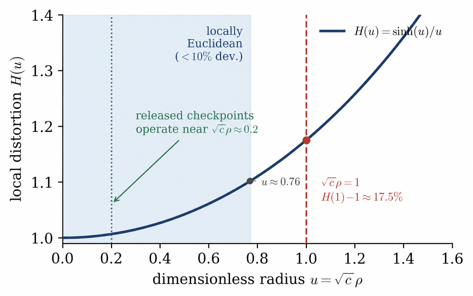
These diagnostics distinguish curvature collapse from geometry use. A model may have small curvature and small radius, resulting in locally Euclidean behavior. It may have small curvature but larger radius, preserving the same effective geometry through the product \(\sqrt{c}\rho\). Or it may enter a regime where \(\sqrt{c}\rho\) is large and \(H(u)\) deviates substantially from one, in which case the radial nonlinearity of hyperbolic geometry is functionally engaged. Our claims concern this effective geometry, not curvature as an isolated scalar.
3.3 Hierarchy diagnostics↩︎
We evaluate three hierarchy notions: lexical taxonomy, visual-semantic granularity, and model-native entailment/order.
3.3.0.1 Radial ordering.
Hyperbolic hierarchy is commonly motivated by a radial interpretation: general concepts should lie closer to the origin and specific concepts farther away. For a directed pair \((p,c)\), where \(p\) is a parent and \(c\) a child, radial consistency is \[\mathrm{RadialOrder}(p,c)= \begin{cases} 1, & \rho_c > \rho_p,\\ 0, & \text{otherwise}, \end{cases}\] where \(\rho_c, \rho_p\) are the child and parent radii and ties are counted as \(0\). We use this as a necessary-condition diagnostic for the radial-depth hypothesis, not as a universal hierarchy metric.
3.3.0.2 Entailment cone activity.
For models using entailment cones, low violation rate alone is not evidence of hierarchy. It may indicate that the model has learned valid order relations, but it may also arise from saturated apertures that make the constraint trivial. We therefore report aperture distributions, active violation rates, directed-pair containment, and, where possible, the gradient contribution of entailment terms (Section 7). When apertures saturate at \(\pi/2\), we interpret zero violation as inactive or trivial entailment rather than as successful hierarchy learning.
3.3.0.3 Traversal robustness.
If a learned representation supports hierarchy, moving along the proposed radial or geodesic direction should produce monotonic semantic changes. We therefore evaluate traversal trajectories by retrieving nearest captions or labels along interpolation paths. We report monotonicity, perfect traversal rate, collapse rate, and diversity of terminal retrievals. Traversal is a model-native diagnostic: it asks whether the representation supports an operational path from general to specific concepts.
3.3.0.4 Product-factor hierarchy.
For PHyCLIP, our goal is not to evaluate factor disentanglement in general. We ask a narrower question: whether individual factors or the product geometry support directed radial ordering or monotonic hierarchical traversal. Factor-wise results are therefore interpreted as hierarchy diagnostics, not as a complete analysis of product-factor semantics.
3.4 Evaluation diagnostics↩︎
Several evaluations can appear hierarchy-sensitive while failing to test the hyperbolic mechanism itself. We therefore separate three sources of signal that hierarchy-looking metrics conflate—angular semantic organization, radial hierarchy, and pair-specific directed structure—and define one diagnostic for each.
3.4.0.1 Angular/radial taxonomy decomposition.
A common hierarchy-looking metric is the correlation between taxonomy distance and embedding distance over class labels. This metric is symmetric: it measures whether semantically related labels are close, but does not determine whether hierarchy is encoded radially. To decompose the signal, we compare a cosine-only regression \[d_{\mathrm{tree}}(i,j) \sim \beta_0 + \beta_1 d_{\cos}(i,j)\] to a cosine-plus-norm regression \[d_{\mathrm{tree}}(i,j) \sim \beta_0 + \beta_1 d_{\cos}(i,j) + \beta_2 \left|\rho_i-\rho_j\right|.\] We report the incremental explanatory power \[\Delta R^2_{\mathrm{norm}} = R^2_{\cos+\mathrm{norm}} - R^2_{\cos}.\] If taxonomy correlation is radial, norm differences should add measurable explanatory power beyond cosine distance. Since pairwise distances are not independent, we use class-level bootstrap or permutation-based procedures rather than treating all class pairs as independent samples.
3.4.0.2 Shuffle-controlled directed tests.
Raw directed norm consistency can be confounded by marginal norm distributions or prompt-length effects. For example, if fine-class prompts have slightly larger norms than their CIFAR-defined superclass prompts, many parent-child inequalities may hold even for random pairings. We therefore compare real directed pairs against shuffle-null controls: \[\Delta_{\mathrm{pair}} = \mathrm{Order}_{\mathrm{real}} - \mathbb{E}_{\mathrm{shuffle}} \left[ \mathrm{Order}_{\mathrm{shuffle}} \right].\] A raw ordering score is not interpreted as hierarchy unless it exceeds the shuffle-null distribution. Where prompt length can affect norms, we use length-matched prompts or residualized norms as sensitivity checks.
As a sanity check, Appendix 14 applies the same radial and shuffle-controlled diagnostics to a synthetic hyperbolic tree with planted radial and angular hierarchy; the diagnostics recover the planted structure and collapse under radius- or angle-shuffled controls.
3.4.0.3 Downstream metrics as decoupling probes.
Retrieval, zero-shot classification, compositional tests, and hierarchy-aware penalties are useful measures of representation quality. However, they do not by themselves establish active hyperbolic hierarchy. We therefore use downstream metrics primarily as decoupling probes: if standard metrics remain comparable or improve while curvature collapses, cones saturate, or radial ordering disappears, then those metrics do not require active hyperbolic hierarchy.
4 Curvature Is Not Separately Identified from Radial Scale↩︎
We first ask whether current hyperbolic VLMs operate in a nonlocal hyperbolic regime. The answer is negative across released checkpoints and controlled interventions. Curvature either binds to the published floor or decreases when the floor is released, while the effective geometry remains near-Euclidean.
4.1 Released checkpoints remain near-Euclidean↩︎
Across released MERU, HyCoCLIP, and PHyCLIP checkpoints, curvature is at the implementation floor or fixed low-curvature setting, consistent with the curvature collapse reported by [13]. However, the more important observation is not the scalar value of \(c\) alone. The effective operating radius \(\sqrt{c}\rho\) remains small across modalities and model families, yielding local distortion factors close to one and zero samples in the nonlocal regime. That curvature and radial scale are interchangeable—the same geometry can be written with large \(c\) and small \(\rho\) or the reverse—is classical for constant-curvature spaces [18], [19]. What we add is the empirical finding that trained hyperbolic VLMs sit at a near-Euclidean operating point, so it is \(\sqrt{c}\rho\), not the scalar \(c\), that characterizes them.
| Model family | Curvature floor | Median \(H(u)\) | Range of \(H(u)\) | % \(\sqrt{c}\rho{>}1\) |
|---|---|---|---|---|
| MERU | \(0.1\) | \(1.009\) | [1.005, 1.014] | \(0\%\) |
| HyCoCLIP | \(0.1\) | \(1.005\) | [1.002, 1.007] | \(0\%\) |
| PHyCLIP | \(0.1\) (per-subspace) | \(1.006\) | [1.003, 1.023] | \(0\%\) |
Table 1 summarizes the released-checkpoint geometry diagnostics. The full per-modality and per-factor table is provided in Appendix 10. Across all released checkpoints, the median local distortion factor is near one, and no model enters the regime \(\sqrt{c}\rho>1\). This holds throughout the distribution, not only at the median: the \(99\)th-percentile and maximum image-side \(\sqrt{c}\rho\) stay at or below \(0.37\) for every released checkpoint, and no sample reaches even the \(\sqrt{c}\rho\approx0.76\) distortion threshold (Appendix 10.2, Table 9). Thus, the released representations do not operate in the nonlocal regime (\(\sqrt{c}\rho>1\)) that motivates hyperbolic hierarchy.
Together, these diagnostics limit the interpretation of curvature collapse. The issue is not merely that \(c\) is small or clamped: the learned embeddings also remain at small dimensionless radius, so the effective operating geometry is close to Euclidean. Notably, the from-scratch current-GRIT baselines converge to the same dimensionless radius as the released checkpoints (\(\sqrt{c}\rho \approx 0.20\) for HyCoCLIP at both scales; Tables 1–2), despite differing in initialization and data availability. The near-Euclidean operating point is thus a recurring empirical regime across these runs rather than an artifact of any single one.
4.2 Unclamping curvature changes parameterization, not geometry↩︎
To test whether the curvature floor is suppressing a useful geometric degree of freedom, we train matched current-GRIT baselines and curvature-unclamped variants. Here “baseline” refers to a model we train from scratch on the current-GRIT snapshot under the published settings. Baseline and clampOff differ only in the curvature clamp. In the clampOff variants, the lower curvature clamp is relaxed from \(0.1\) to \(0.001\), while all other training settings are kept fixed. Controlled interventions are run at ViT-S and ViT-B. ViT-L is audited only at the released-checkpoint level (Table 8).
| \(c\) | \(\rho\) | \(\sqrt{c}\,\rho\) | \(H(u)\) | |||||
|---|---|---|---|---|---|---|---|---|
| 2-3(lr)4-5(lr)6-7(lr)8-9 Model | baseline | clampOff | baseline | clampOff | baseline | clampOff | baseline | clampOff |
| MERU-S | \(0.1000\) | \(0.0419\) | \(0.921\) | \(1.052\) | 0.291 | 0.215 | 1.014 | 1.008 |
| MERU-B | \(0.1000\) | \(0.0289{\scriptstyle\pm.0007}\) | \(0.939{\scriptstyle\pm.004}\) | \(1.049{\scriptstyle\pm.003}\) | \(0.297{\scriptstyle\pm.001}\) | \(0.178{\scriptstyle\pm.002}\) | \(1.015{\scriptstyle\pm.000}\) | \(1.005{\scriptstyle\pm.000}\) |
| HyCoCLIP-S | \(0.1000\) | \(0.0112\) | \(0.635\) | \(1.839\) | 0.201 | 0.194 | 1.007 | 1.006 |
| HyCoCLIP-B | \(0.1000\) | \(0.0093{\scriptstyle\pm.0003}\) | \(0.638{\scriptstyle\pm.000}\) | \(2.019{\scriptstyle\pm.030}\) | \(0.202{\scriptstyle\pm.000}\) | \(0.195{\scriptstyle\pm.000}\) | \(1.007{\scriptstyle\pm.000}\) | \(1.006{\scriptstyle\pm.000}\) |
| PHyCLIP-S | \(0.1000\) | \(0.0155\) | \(0.644\) | \(1.508\) | 0.204 | 0.188 | 1.007 | 1.006 |
| PHyCLIP-B | \(0.1000\) | \(0.0144{\scriptstyle\pm.0001}\) | \(0.650{\scriptstyle\pm.000}\) | \(1.562{\scriptstyle\pm.008}\) | \(0.206{\scriptstyle\pm.000}\) | \(0.187{\scriptstyle\pm.000}\) | \(1.007{\scriptstyle\pm.000}\) | \(1.006{\scriptstyle\pm.000}\) |
4pt
Table 2 shows the central result. Releasing the curvature floor changes \(c\) and embedding norms, but does not move the models into a nonlocal hyperbolic regime. The effect on the dimensionless radius is family-dependent. In HyCoCLIP, \(c\) decreases by roughly an order of magnitude and norms increase, preserving \(\sqrt{c}\rho\) to within about \(3.5\%\). In MERU, the compensation is incomplete and unclamping moves the model to an even lower dimensionless radius. PHyCLIP falls between the two. In every case, however, the model stays well inside the near-Euclidean regime: across all families and sizes in these current-GRIT runs the local distortion factor remains at or below \(1.015\) and the nonlocal-regime fraction remains \(0\%\) (Figure 2).

4.3 Downstream metrics remain comparable under curvature collapse↩︎
If curvature were a performance-critical resource, relaxing the floor should substantially alter downstream behavior. Instead, standard metrics remain comparable when the geometry moves to near-Euclidean.
| Downstream (\(\Delta\)) | WordNet hierarchy (\(\Delta\)) | ||||||||||
|---|---|---|---|---|---|---|---|---|---|---|---|
| 2-7(lr)8-12 Model | T2I COCO | I2T COCO | T2I Flk | I2T Flk | ZSC IN | SC | TIE\(\downarrow\) | LCA\(\downarrow\) | J\(\uparrow\) | PH\(\uparrow\) | RH\(\uparrow\) |
| MERU-B | \(-0.04{\scriptstyle\pm0.48}\) | \(-0.47{\scriptstyle\pm0.23}\) | \(-0.05{\scriptstyle\pm0.17}\) | \(+0.00{\scriptstyle\pm0.89}\) | \(-0.46{\scriptstyle\pm0.24}\) | \(+0.12{\scriptstyle\pm0.12}\) | \(+0.049{\scriptstyle\pm0.039}\) | \(+0.007{\scriptstyle\pm0.021}\) | \(-0.0038{\scriptstyle\pm0.0025}\) | \(-0.0016{\scriptstyle\pm0.0019}\) | \(-0.0036{\scriptstyle\pm0.0024}\) |
| HyCoCLIP-B | \(+0.96{\scriptstyle\pm0.63}\) | \(+1.60{\scriptstyle\pm0.43}\) | \(+0.72{\scriptstyle\pm0.40}\) | \(+1.00{\scriptstyle\pm0.56}\) | \(-0.35{\scriptstyle\pm0.29}\) | \(+1.36{\scriptstyle\pm0.22}\) | \(+0.084{\scriptstyle\pm0.027}\) | \(+0.029{\scriptstyle\pm0.028}\) | \(-0.0053{\scriptstyle\pm0.0016}\) | \(-0.0033{\scriptstyle\pm0.0019}\) | \(-0.0053{\scriptstyle\pm0.0012}\) |
| PHyCLIP-B | \(+0.64{\scriptstyle\pm0.22}\) | \(+0.63{\scriptstyle\pm0.48}\) | \(+0.43{\scriptstyle\pm0.35}\) | \(+0.17{\scriptstyle\pm0.65}\) | \(-0.29{\scriptstyle\pm0.61}\) | \(+0.76{\scriptstyle\pm0.79}\) | \(+0.049{\scriptstyle\pm0.030}\) | \(+0.003{\scriptstyle\pm0.022}\) | \(-0.0041{\scriptstyle\pm0.0016}\) | \(-0.0019{\scriptstyle\pm0.0016}\) | \(-0.0040{\scriptstyle\pm0.0009}\) |
4pt
Table 3 reports current-GRIT matched comparisons for MERU-B, HyCoCLIP-B, and PHyCLIP-B. The positive HyCoCLIP-B deltas are consistent across all three seeds, but we read these structural interventions as decoupling evidence—performance does not degrade when curvature collapses—not as a claim that clampOff is a better or significantly improved model. The decoupling is direct. For HyCoCLIP-B clampOff, curvature drops by an order of magnitude to \(c\approx0.009\) and the representation becomes near-Euclidean, yet COCO and Flickr [23] retrieval and SugarCrepe [24] move in the positive direction relative to baseline, while ImageNet zero-shot (\(-0.35{\scriptstyle\pm0.29}\)) and VL-Checklist [25] shift within the seed spread. (VL-Checklist is positive at seed 0 but seed-variable, with a three-seed mean ranging from \(-0.5\) to \(-4.3\) points across subtypes.) Four of the five WordNet [26] hierarchical metrics (TIE, J, PH, RH) shift by small but consistent-sign amounts (e.g.TIE \(+0.084{\scriptstyle\pm0.027}\)); none shows substantial degradation across the three seeds. For MERU-B these metrics show only small shifts (\(\leq0.5\) points, some sign-consistent) across the three matched seeds. PHyCLIP-B likewise shows only small shifts under clampOff, with retrieval and SugarCrepe moving in the positive direction, the ImageNet metric within the seed spread, and the WordNet hierarchy metrics again shifting by small, consistent-sign amounts (e.g.RH) of negligible magnitude. Across all three families, collapsing curvature toward the Euclidean regime does not cost substantial downstream performance in this matched setting: the WordNet hierarchy metrics carry a small, consistent-sign cost of negligible magnitude, while the core retrieval, zero-shot, and compositionality metrics are flat to positive. This conclusion is scoped to the regime we can reach: both the baseline and the clampOff models already operate near-Euclidean (\(\sqrt{c}\rho\approx0.2\)–\(0.3\)), so within that regime curvature is not separately performance-critical. We cannot probe a stable trained high-curvature regime in the audited final checkpoints: early training transients can enter \(\sqrt{c}\rho>1\), but every converged audited configuration contracts to the near-Euclidean band—and that contraction is itself one of our findings, not a gap in the comparison.
Released checkpoints often obtain higher absolute downstream scores than current-GRIT baselines. We treat them as historical references only, since they may differ in data availability.
Together, these results indicate that curvature is not identifiable separately from radial scale: across families, sizes, and floor settings, the operating point \(\sqrt{c}\rho\) stays in the same near-Euclidean range (\(\approx 0.2\)–\(0.3\)), whether the curvature change is absorbed by compensating norm growth (HyCoCLIP, which nearly preserves \(\sqrt{c}\rho\)) or only partially compensated (MERU, where \(\sqrt{c}\rho\) falls further). In either case it is the combination \(\sqrt{c}\rho\), not the scalar \(c\), that governs the operating geometry (Tables 1–2). Curvature moves, but because the operating point either holds or drops rather than entering the nonlinear regime, the scalar \(c\) is not separately recoverable from downstream behavior. This identifies the first of two distinct failures. Curvature is not the active geometric resource in any audited configuration: no converged run remains in the nonlinear hyperbolic regime. This does not by itself imply that hierarchy is absent: radial depth ordering can in principle be expressed even in a near-Euclidean space [9], [10], so the two failures are logically separable—flatness does not entail the absence of order—even though, as Sections 7.3–7.4 argue, they may share related objective-level causes—the entailment shortcut and the absence of a curvature-identifying contrastive/alignment signal.
We therefore ask separately, in the next section, whether the hierarchy mechanism the geometry motivates appears anywhere in the representation—in radial ordering, cone activity, or traversal—regardless of curvature.
5 Direct Diagnostics Do Not Detect an Operative Hierarchy↩︎
We distinguish lexical hierarchy, model-native cone/order structure, and operational traversal. Across these diagnostics, no audited formulation shows evidence of an operative, graded directed radial or cone-based hierarchy.
5.1 External radial ordering is not detected; native structure is detectable but non-operative↩︎
Hyperbolic VLMs are motivated by the radial-depth hypothesis: general concepts should be closer to the origin and specific concepts farther away. We evaluate this hypothesis using directed parent–child pairs given by the CIFAR-100 [27] fine\(\to\)coarse label hierarchy: each fine class is paired with its CIFAR-defined superclass, yielding 100 (parent\(=\)coarse, child\(=\)fine) pairs. WordNet is not used to construct these pairs. It enters only in Section 6.1 for the taxonomy-distance correlation. For each pair, we ask whether the child embedding has larger norm than the parent embedding, and we compare the resulting consistency against a shuffle-null distribution over randomly permuted pairings, following the criterion of Section 3.4.
A raw norm-ordering rate can be driven by a marginal effect—all specific prompts being larger-normed than all general ones on average—which need not reflect any learned parent-child relation: it can arise from prompt length, level marginals, or a global specific-versus-general norm offset. The shuffle null removes exactly this marginal component, leaving the pair-specific question: do true parent-child pairings carry more radial order than exchangeable pairings with the same norm marginals? This pair-specific version matches the radial-hierarchy claim these models actually make—a child sits deeper than its own parent, not merely deeper than the average parent—so we take the pair-specific excess as the honest target throughout.
Across released checkpoints, no hyperbolic family’s parent-child norm consistency exceeds its shuffle null (Figure 3). MERU, HyCoCLIP, and PHyCLIP all fall within the non-detection band (\(|z|<1.6\)) of their shuffle nulls. The only checkpoint to cross it is the Euclidean CLIP baseline (\(z=+1.73\)), which by construction encodes no radial hierarchy, so its crossing marks the noise floor rather than a radial signal. Nor does any fall significantly below its null (most negative: PHyCLIP, \(z=-0.67\)). By the shuffle-controlled criterion, none of the hyperbolic models uses the radial coordinate as a reliable semantic-depth axis. The same holds at the remaining released scales: every ViT-S checkpoint and both ViT-L hyperbolic checkpoints stay within the band, the largest excursion being PHyCLIP-L (\(z=-1.59\)).
This non-detection is bounded, not a power artifact: a graded positive control matched to the diagnostic’s design (same \(100\) pairs and shuffle procedure) recovers a planted pair-specific radial ordering at \(80\%\) power once its shuffle-controlled excess reaches \(\Delta_{\mathrm{pair}}\approx13\) percentage points (Appendix 14.1), and every audited model stays well below this sensitivity—the largest absolute shuffle-controlled gap among released checkpoints is about \(5\) pp (PHyCLIP-L), the other hyperbolic released models within about \(2\) pp, so even the Euclidean CLIP-B crossing is a sub-detection-magnitude artifact. Across the current-GRIT runs, individual seeds cross \(\pm1.6\) in either direction, but no model’s three-seed mean exceeds the threshold in the radial-depth direction, the positive single-seed excursions are seed-inconsistent at the per-seed false-positive rate (the one seed-consistent pattern, PHyCLIP-B baseline’s below-null \(z\approx-2\), points against radial hierarchy and does not survive correction), and—decisively—every such model fails the operative graded traversal (Section 5.3). Full results are in Table 29.

This is not to say the models lack semantic structure. They may still encode angular semantic similarity. Sibling or related concepts can be close in angle. The point is narrower: on this external taxonomy the radial coordinate is not aligned with the parent-child abstraction direction, in any family, above chance (the native relation is treated separately just below, where a small detectable-but-non-operative residual does appear).
5.1.0.1 A model-native relation test partially qualifies this result.
The diagnostic above uses the CIFAR-100 fine\(\to\)coarse label hierarchy, an external taxonomy rather than the relation the box-supervised models were trained on. We therefore repeat the directed radial test on the native GRIT box\(\to\)full caption structure (hereafter NG2). Each sample pairs a full-image caption (the more specific concept, predicted to have larger norm) with its box-level captions (the more general concept, predicted smaller), following HyCoCLIP’s compositional convention [2]. We use the same shuffle-controlled estimand as the external test above, with a sample-level null that re-pairs each full caption with boxes from other samples, preserving the marginal norm distributions of fulls and boxes so that only pair-specific structure survives (\(n=1000\) pairs, \(R=500\) permutations). We control caption length (a length-matched subset with \(|\Delta\text{tok}|\le3\) and a length-residualized variant) and partial out cosine distance, as in Section 6.1.
After these controls, angular distance remains the dominant predictor in every model, and a radial supplement beyond cosine is at most small. On the released checkpoints it is negligible: \(\Delta R^2_{\mathrm{norm}}\le0.00040\) across the released ViT-B checkpoints (PHyCLIP-B not distinguishable from zero, \(p=0.41\); the largest, MERU-B, is \(0.00040\)), consistent with the external-taxonomy null above. Under the clampOff checkpoints it is larger but seed-unstable—spanning \(0\)–\(0.0023\) for HyCoCLIP-B (Mantel-significant at two of three seeds, indistinguishable from zero at seed 42, \(p=0.285\)) and \(0.00016\)–\(0.00035\) for PHyCLIP-B (significant at all three; Table 30)—whereas the directed one-bit signal is seed-robust (full-set \(z\) between \(+7.6\) and \(+10.0\)), so what varies with seed is precisely the graded component an active radial axis would require. Even the largest supplement (\(0.0023\), HyCoCLIP-B clampOff seed 37) is only \(0.23\%\) of total distance variance on the native relation.
Three bounds scope this reading. The released-versus-clampOff difference is cross-sectional, not a matched intervention, so it cannot determine whether removing the floor reveals or rescales the supplement. The sample-level null preserves the full/box norm marginals, so a within-sample visual-specificity gap that length-matching does not capture could produce the norm ordering without any graded depth coordinate. And a significant directed \(z\) certifies only a single reliable bit—that a full caption tends to sit outside its own box (\(z\approx+8.4\)–\(+9.7\) for the box-trained models, \(+9.3\) for MERU-B despite no box supervision, all far above Euclidean CLIP-B’s \(+3.0\))—not the graded axis the mechanism claims: the cosine-controlled increment is \(\Delta R^2_{\mathrm{norm}}\approx0\) and strict traversal monotonicity is \(0\%\). The negative result is thus refined rather than overturned: no operative radial axis under either the external or the native test, and a small, statistically detectable native supplement that remains secondary to angular structure and below what an active radial hierarchy would require.
We verify the detectable-versus-operative distinction directly on the NG2 relation under three retrieval readouts (Appendix 13.5, Tables 31 and 32). Stepping outward along the radial coordinate with the angle held fixed returns an essentially constant caption—a methods fact rather than model evidence: this readout uses cosine retrieval, which is norm-invariant, so its \(\approx0\) rank correlation cannot expose a radial axis in any model. A geodesic (ambient straight-line) readout does produce a positive correlation, but two controls show it is generic to straight-line interpolation rather than a hyperbolic-hierarchy signature. First, a mismatched-target variant stays well above the shuffle null. Second, the Euclidean CLIP baseline produces the largest geodesic correlation of all seven models (\(\rho=0.71\)), exceeding every box-trained hyperbolic checkpoint—despite having no radial structure, since it fails the per-pair direction precheck at chance (distinct from the pooled \(z\)) and its cosine-controlled increment is negligible. The NG2 direction therefore carries a strong pairwise norm signal but no operative abstraction axis under any informative readout: positive-but-generic under the controlled geodesic readout, never strictly monotonic, and with a cosine-controlled radial increment of \(\approx0\). Full per-model values are in Appendix 13.5.
5.2 Entailment cones are inactive, saturated, or misaligned↩︎
Entailment cones are intended to encode asymmetric semantic order. However, the observed cone behavior is fragile. Under the default threshold, some intra-modal entailment terms are almost trivially satisfied and provide little effective gradient. The text-side cone is already saturated at \(\pi/2\) at baseline in every family, so the text\(\to\)image violation rate is low to begin with (\(0\)–\(0.4\%\) for the current-GRIT HyCoCLIP baselines, \(2.7\)–\(5.1\%\) for MERU; \(9\)–\(14\%\) for PHyCLIP at baseline, where larger image norms place some embeddings just outside the saturated cone). Under clampOff the PHyCLIP rate collapses (\(\le0.2\%\)) as embedding norms compress, while MERU’s stays in low single digits and HyCoCLIP’s at zero. Under clampOff the image-side aperture often saturates too—with MERU near the saturation edge as the exception discussed below—yet the image\(\to\)text rate stays pinned near \(100\%\) because text embeddings still fall outside the (now \(\pi/2\)) cone. Either way the cone constraint is vacuous rather than satisfied, so a low or zero violation rate evidences cone trivialization, not learned semantic hierarchy. Conversely, when entailment thresholds are tightened, violation rates become high but the geometry and traversal diagnostics remain unchanged.
Table 4 summarizes representative cone behavior. In HyCoCLIP, the text-side cone is saturated already at baseline (text\(\to\)image violation \(0\%\)) and stays saturated under clampOff, so the vacuous constraint is the baseline condition rather than a clampOff-induced drop. The image-side cone additionally saturates under clampOff (\(11\%\to100\%\) image-side), but the image\(\to\)text violation stays at \(100\%\) as text embeddings continue to fall outside the cone. MERU shows that non-saturation fails just as completely: its image-side apertures remain geometrically non-saturated at baseline (\(0.73\) rad), yet text embeddings fall outside the active image cone in virtually every sample (image\(\to\)text violation rate near 100% on matched GRIT pairs). Under clampOff MERU sits right at the saturation edge—MERU-B saturates to \(\pi/2\) at all three seeds, while MERU-S remains non-saturated (\(1.175\) rad)—the knife-edge regime at the saturation edge (Section 7.3). The cone is thus geometrically active without the embeddings entering it—a saturated aperture and a near-empty one fail for opposite reasons but with the same outcome. Neither non-saturation nor zero violation is therefore sufficient evidence of operational hierarchy. We show in Section 7.3 that this is not incidental: the entailment objective itself admits a low-curvature solution that widens apertures and suppresses violations without learning semantic order. Low violation rates must therefore be interpreted jointly with aperture and gradient diagnostics.
This pattern is family-universal. PHyCLIP shows the same image-cone signature as MERU—text embeddings never enter the active image cone (image\(\to\)text violation \(\approx100\%\) at both baseline and clampOff), regardless of saturation state. A second, distinct signal appears on the text-cone side: PHyCLIP image-side apertures saturate from \(41\)–\(45\%\) at baseline to \(\approx96\%\) under clampOff, and in the same clampOff transition embedding norms compress so that the text–image angle distribution shrinks, driving the complementary text\(\to\)image violation rate down per size (PHyCLIP-S \(13.8\%\to0.2\%\), PHyCLIP-B \(9.5\%\to0.05\%\); Appendix 10.4). The image-side saturation and this text\(\to\)image collapse are co-symptoms of the same curvature collapse rather than one causing the other—saturation acts on the image-cone (image\(\to\)text) test while embedding compression acts on the text-cone (text\(\to\)image) test—and both routes leave the cone unable to encode order, the aperture-saturation signature we trace to the low-curvature shortcut in Section 7.3, now visible across all three families (the per-loss gradient decomposition is probed directly for MERU and HyCoCLIP; for PHyCLIP we observe the aperture signature rather than decomposing its gradients).1 Across both saturation regimes the cone fails to encode learned order—the image-side constraint is non-informative (text never enters the image cone), the text-side rate reflects embedding compression rather than order. Full per-model diagnostics are in Appendix 10.4.
| Model | Image aperture | Text aperture | Interpretation |
|---|---|---|---|
| MERU-B baseline | \(0.73\) rad | \(\pi/2\) saturated | Image-side cones are geometrically non-saturated, but traversal still collapses. |
| MERU-B clampOff | \(\pi/2\) saturated | \(\pi/2\) saturated | Saturated at all three seeds, settling just below the \(2K\) edge (Section [sec:sec:entailment95shortcut]); no operational hierarchy. |
| MERU-S clampOff | \(1.175\) rad | \(\pi/2\) saturated | Operating point above the edge (\(\sqrt{c}\rho=0.217>2K\), single seed); the non-saturated image cone is consistent with the edge criterion (Section [sec:sec:entailment95shortcut]). |
| HyCoCLIP-B baseline | \(1.42\) rad | \(\pi/2\) saturated | Cone constraints remain nontrivial but do not yield traversal hierarchy. |
| HyCoCLIP-B clampOff | \(\pi/2\) saturated | \(\pi/2\) saturated | Both saturate; t\(\to\)i constraint vacuous (\(\approx0\)), i\(\to\)t at \(100\%\)—inactive either way. |
5.3 Traversal collapses instead of moving along hierarchy↩︎
A stronger operational test is traversal. If radial or geodesic movement corresponds to abstraction, then traversing the learned space should produce monotonic semantic changes. Instead, traversal collapses across families, scales, and factors (summarized across interventions in Table 19).
Across MERU and HyCoCLIP current-GRIT baselines, norm monotonicity is low, perfect monotonic traversal is never observed, and terminal retrievals collapse to a single or very small set of captions. For these external-pool walks, retrieval at each interpolation step uses the model’s own metric—Lorentz distance for the hyperbolic models, not the norm-invariant cosine (the native-relation readouts of Appendix 13.5 use cosine)—and monotonicity denotes the per-step fraction of steps moving in the predicted specific\(\to\)general direction (chance \(50\%\)). Steps on which the retrieved caption is unchanged—frequent under the hub collapse below—count against monotonicity, so the raw rate conflates wrong-direction moves with sticky no-moves. Perfect traversal is a trajectory-level statistic whose random baseline is far lower (\({\approx}2^{-K}\) for \(K\) steps), so \(0\%\) perfect traversal is conservative against either reference. In current-GRIT interventions, the same pattern appears: curvature unclamping changes \(c\) and norms, but traversal remains collapsed. PHyCLIP requires a stronger check because its hierarchy may be distributed across product factors rather than visible only in the aggregate representation. We therefore evaluate each of the 64 factors separately. The result is uniformly negative: across PHyCLIP-B and PHyCLIP-L, and across ImageNet, COCO, and Flickr30k retrieval pools, no factor exceeds the \(50\%\) per-step reference and no factor achieves a perfect traversal (Table 21). The aggregate (full product-distance) representation fares no better, with monotonicity in the \(8\)–\(19\%\) range, like the per-factor mean (\(21.3\)–\(25.6\%\)). Since sticky no-move steps depress these raw rates, we read them as corroborating rather than load-bearing. Thus neither the aggregate representation nor any individual factor supports monotonic hierarchical traversal, and the product factorization does not reveal hidden monotonic hierarchy at either level.
Qualitative traversal examples can therefore mislead: early steps may retrieve paraphrases or visually related captions, but systematic traversal reveals a later collapse phase in which trajectories converge to a few hub captions. This is not COCO-specific—on HyCoCLIP’s own Flickr30k demo pool [2], \(200\) image\(\to\)root traversals on the released HyCoCLIP-B reach only \(13\) distinct terminals, \(79\%\) funnelling into two degenerate hubs (Appendix 12.3). Low monotonicity and terminal collapse are the per-step and terminal views of the same step-wise stickiness.
Because that stickiness registers as ties, the evidence hierarchy is as follows. Load-bearing: the graded geodesic readout with its mismatched-target and Euclidean controls—on which the Euclidean CLIP baseline attains the largest correlation of all seven models (\(\rho=0.71\)), so positive geodesic movement is generic to straight-line interpolation rather than hyperbolic hierarchy—together with the near-zero cosine-controlled radial increment (Tables 32, 30). Corroborating: the tie-confounded per-step monotonicity. Symptomatic and pool-dependent: terminal collapse (Appendix 12.3). The per-step monotonicity is pool-independent (structured label and relation pools keep diverse terminals yet still fail it) and corroborates these. Under every readout, and independent of the retrieval pool, the trajectories do not realize an operational hierarchy from general to specific concepts.
5.4 Threshold changes affect regularization, not hierarchy↩︎
Finally, we test whether activating intra-modal entailment by changing the threshold \(\eta\) recovers hierarchy. Lowering \(\eta\) from \(1.2\) to \(0.7\) changes downstream metrics in a scale-dependent way, but leaves curvature at the floor, the local distortion factor near one, and traversal collapsed. We report the full intervention in Appendix 11.3. Taken together, the radial, cone, and traversal diagnostics find no evidence of the radial/cone mechanism in the representation, and the natural threshold intervention does not install it. Yet prior work has reported hierarchy-like signals from these same models. The next section asks what those evaluations measure.
6 Hierarchy-Looking Evaluations Are Underdetermined↩︎
The previous section shows that direct hierarchy diagnostics fail. We now ask why prior evaluations can nevertheless suggest that hyperbolic VLMs are more hierarchical. We find that several hierarchy-looking metrics are underdetermined: they capture useful angular semantic organization or bulk norm effects, not directed radial hierarchy.
6.1 Taxonomy-distance correlation is angular rather than radial↩︎
Prior work reports that hyperbolic VLMs can show stronger correlations between taxonomy distance and embedding distance. We reproduce this qualitative positive signal on CIFAR-100. Hyperbolic checkpoints obtain higher WordNet path-distance correlations than Euclidean CLIP across all sizes. Multiple hyperbolic variants exceed \(r \approx 0.45\), with HyCoCLIP-B clampOff reaching the strongest correlation (\(r = 0.510\) at seed \(0\)) despite its curvature collapsing to \(c \approx 0.009\) (Table 28).
| Model | Setting | Taxonomy \(r\) | \(R^2_{\cos}\) | \(R^2_{\mathrm{norm\text{-}only}}\) | \(\Delta R^2_{\mathrm{norm}}\) | \(p_{\mathrm{perm}}\) |
|---|---|---|---|---|---|---|
| CLIP-B | released | 0.370 | 0.137 | 0.001 | +0.003 | 0.25 |
| MERU-B | released | 0.489 | 0.239 | 0.001 | +0.001 | 0.34 |
| HyCoCLIP-B | released | 0.465 | 0.217 | 0.005 | +0.001 | 0.50 |
| PHyCLIP-B | released | 0.456 | 0.208 | 0.002 | +0.000 | 0.74 |
| PHyCLIP-L | released | 0.456 | 0.208 | 0.003 | +0.001 | 0.50 |
| HyCoCLIP-B | baseline | 0.462 | 0.214 | 0.001 | +0.002 | 0.44 |
| HyCoCLIP-B | clampOff | 0.508 | 0.258 | 0.001 | +0.001 | 0.44 |
However, a stronger correlation need not reflect active radial hierarchy. Table 5 decomposes the signal into angular and radial components, reporting both the norm-only regression \(R^2_{\mathrm{norm\text{-}only}}\) and the incremental \(\Delta R^2_{\mathrm{norm}} = R^2_{\cos+\mathrm{norm}} - R^2_{\cos}\). Cosine distance explains the taxonomy correlation, while norm differences add no detectable explanatory power beyond cosine: the norm-only \(R^2\) is small in isolation (\(\leq 0.007\)) and the incremental \(\Delta R^2_{\mathrm{norm}} \leq 0.003\) across the decomposed models. Mantel permutation tests detect no significant norm contribution at \(\alpha = 0.05\) in any of the 44 model\(\times\)mapping combinations we evaluate (minimum \(p_{\mathrm{perm}} = 0.125\); full per-model \(r\) and Mantel \(p\) values are in Table 27). The decomposition is unchanged under either WordNet mapping—the manually disambiguated synsets used here, or the naive last-token heuristic: Pearson \(r\) shifts by \(0.01\)–\(0.10\) but \(\Delta R^2_{\mathrm{norm}}\leq0.003\) throughout (Appendix 13.1, Table 27). The decomposition runs over same-level leaf pairs, where radial depth differences are structurally small. It bounds the radial share of the leaf-level taxonomy signal, not depth coding in general. A sensitivity analysis bounds the null: the largest audited seed-mean increment (MERU-B baseline, \(0.0029\); per-seed values reach \(0.0054\), still \(2.4\times\) below threshold) sits at the Euclidean CLIP noise floor and more than four times below the \(\approx0.013\) detectability threshold (Appendix 14.1; Table 28), and the same analysis shows a norm signal that merely re-encodes the coarse partition is undetectable because cosine already captures it—norm–cosine redundancy, not an absence of norm structure per se.
This reconciles prior positive evidence with our diagnostics. Hyperbolic VLMs can learn useful angular semantic structure, and this can improve symmetric taxonomy-distance correlation. But symmetric semantic distance is not the same as directed radial hierarchy.
6.2 Directed norm scores require shuffle controls↩︎
Raw directed norm-ordering scores can also mislead: a marginal norm offset—specific prompts being higher-norm than general ones on average—inflates the apparent ordering even without any learned parent–child structure, which is why our radial diagnostic (Section 5.1) reads directed consistency only against a shuffle null rather than as a raw rate. Under that control, no audited model’s directed score survives above chance on the external CIFAR-100 fine\(\to\)coarse hierarchy (Figure 3, Table 29). The only surviving signal is the small pair-specific residual on the models’ own native relation (Section 5.1). Published evidence of this form—e.g., the observation that box embeddings sit closer to the origin than full-image embeddings [2]—is exactly what the null control adjudicates: its pair-specific component is real (Table 30, \(z\approx+9.7\)) but remains secondary to angular structure and non-operative as a hierarchy readout.
The lesson generalizes beyond our own diagnostic: any directed-looking norm score must be reported against a null control. Without one, a model can appear hierarchy-like purely because of marginal prompt statistics rather than learned parent-child relations—a confound that, as Section 5.1 shows, accounts for essentially all the apparent directed signal on that external hierarchy in current hyperbolic VLMs.
6.3 Leaf-level benchmarks do not validate hyperbolic hierarchy↩︎
Many standard benchmarks used to validate VLMs are leaf-level discrimination tasks. ImageNet classification, for example, evaluates separation among leaf classes, not abstraction across levels. Hierarchy-aware penalties such as TIE or LCA incorporate taxonomy into scoring, but improved scores can be driven by angular semantic similarity among related leaves rather than by directed radial hierarchy.
Following the decoupling logic of Section 3.4, these leaf-level and hierarchy-aware scores cannot by themselves establish active hyperbolic hierarchy: a model can improve on them while geometry remains near-Euclidean and our direct hierarchy diagnostics fail.
6.4 Multi-granularity retrieval separates supervision from geometry↩︎
We evaluate retrieval across WordNet abstraction depths using ancestor-defined query centroids—each formed by averaging the embeddings of an ancestor concept’s descendant leaf classes—against ImageNet validation images. This test is more hierarchy-sensitive than leaf-level classification: coarse queries should retrieve broad semantic groups, while fine queries should retrieve narrow leaf-level classes.
The retrieval picture varies sharply with abstraction depth. At the coarsest levels, all models remain weak in absolute terms: for the root-like entity level (depth \(1\), only two qualifying queries), even the best AP is \(0.128\). At fine depths (\(d \geq 11\)) the four families are nearly tied at matched scale (ViT-B: AP \(0.57\)–\(0.60\)). At coarse depths (\(d \leq 5\)), however, HyCoCLIP and PHyCLIP substantially outperform CLIP and MERU at every scale, reaching AP \(\approx0.33\)–\(0.34\) at ViT-B compared to \(0.18\)–\(0.19\) for the non-box-supervised models.
This coarse-depth advantage is not produced by active nonlocal hyperbolic geometry, on two independent grounds. First, hyperbolic geometry alone does not deliver it: the one hyperbolic-but-non-box model, MERU, stays close to Euclidean CLIP at coarse depths across ViT-S/B/L, while only the box/compositional HyCoCLIP and PHyCLIP improve substantially (Table 34; Appendix 15). Second, the winning models sit at a near-Euclidean operating point and fail every activity diagnostic—external radial ordering, cone activity, and traversal—so we find no evidence that their hyperbolic mechanism contributes to the gain. The advantage thus reflects stronger angular semantic organization from compositional supervision, not radial depth. The models’ native box-caption radial residual is real but tiny and non-operative. We do not isolate box supervision from other pipeline differences. The gain tracks the box/compositionally supervised families.
Across Sections 6.1–6.4, the same pattern recurs: each hierarchy-looking signal, once decomposed or controlled, reduces to angular semantic organization, marginal prompt statistics, or box/compositional supervision rather than active radial geometry. Sections 4 and 5 showed the radial/cone mechanism is not activated and goes undetected under our diagnostics. This section shows the positive evidence for it was underdetermined. What remains is the mechanistic question: given that curvature collapses and the cones fail to encode order, why do the natural interventions meant to install hierarchy fail to do so? Section 7 answers this by tracing the gradients that move curvature and by ablating the entailment term to test whether the contrastive/alignment objective can stabilize a nonlocal operating point.
7 Why Simple Interventions Fail↩︎
The previous sections show that current models neither enter the nonlocal hyperbolic regime nor exhibit the radial/cone hierarchy under our diagnostics. We now ask the mechanistic question: why do the natural interventions meant to install hierarchy fail? We examine these routes in order of increasing directness. Two fail analytically: pairwise depth ranking has no direct curvature gradient (Section 7.1), and naive curvature-coupled depth supervision opens a norm-growth escape route (Section 7.2). The central result (Section 7.3) is that the hierarchy-motivated entailment objective itself admits a low-curvature shortcut, so curvature collapse is better explained as a property of the loss than an optimization accident. A c-only diagnostic traces the dominant curvature-lowering pressure on the full-objective trajectory to the entailment term. An entailment-off ablation (Section 7.4) then shows the shortcut is not the only route to low curvature—the contrastive/alignment objective alone also fails to stabilize a nonlocal operating point—while activating the entailment term more strongly (Appendix 11.3) likewise does not install hierarchy.
7.1 Pairwise depth ranking has no direct curvature gradient↩︎
A natural intervention is to add a pairwise depth-ranking loss encouraging deeper concepts to have larger radii. However, if this loss is defined only on embedding norms, it has no direct dependence on curvature: \[L_{\mathrm{depth}} = \max(0, m - (\rho_c-\rho_p)).\] Therefore \(\partial L_{\mathrm{depth}}/\partial c=0\). In from-scratch training, this loss can change norms but cannot identify curvature.
7.2 Naive curvature coupling opens a norm-growth escape route↩︎
A second intervention is to couple depth supervision to the dimensionless radius, for example by replacing the score with \(\sqrt{c}\rho\). This creates a direct curvature path, but it also opens an uncontrolled norm-growth path: \(\sqrt{c}\rho\) can be increased either by raising the curvature \(c\) or by growing the embedding norm \(\rho\), so a model under such supervision can satisfy the depth objective by inflating norms rather than by adjusting curvature, leaving the curvature collapse unaddressed.
This does not mean curvature-coupled objectives are impossible in principle. It shows that curvature-coupled hierarchy supervision must be paired with explicit radial-growth control. Without such control, the depth objective is satisfiable by norm growth alone. This is precisely the path our c-only diagnostic (Section 7.3) removes, by detaching the norm so that the depth gradient reaches curvature directly.
7.3 The entailment loss has a low-curvature shortcut↩︎
The first two interventions fail for fixable reasons—one lacks a curvature gradient, the other lacks norm control. The third reveals a deeper obstacle: even when a curvature gradient is present and norm growth is blocked, the entailment objective itself drives curvature down. This mechanism helps explain the negative results in Sections 4–5, and we isolate it directly in the probed checkpoints and batches.
To separate curvature identification from radial norm growth, we run a c-only diagnostic: \[h = \sqrt{c}\,\mathrm{stopgrad}(\rho).\] This preserves a direct gradient from the depth objective to curvature while blocking the depth loss from changing feature norms. The diagnostic is not a hierarchy-learning method. It tests whether a depth signal can identify curvature once the norm-growth path is removed. We stress that depth supervision is not part of the training objective of any audited model. The depth gradient is measured purely as a counterfactual. We report it only for HyCoCLIP, whose depth pairs come from box-level parent captions. MERU has no box-level supervision, so the same counterfactual is not comparable there.
The implementation was verified to be additive rather than ratio-based, so \(\sqrt{c}\) does not cancel. Finite differences confirm a nonzero curvature gradient. Nevertheless, curvature still collapses to the floor. A per-loss gradient decomposition reveals why. In representative full-objective checkpoints and batches, the contrastive term pushes curvature upward while it carries signal, whereas the entailment term pushes curvature downward by a comparable or (usually) larger magnitude. We use this diagnostic as a mechanism probe, not a population-level estimate: absolute magnitudes vary across checkpoints and batches, but the entailment c-down sign is consistent throughout the collapse phase, and, on the full-objective trajectory, the contrastive c-up sign is reliable until the gradient vanishes to noise near the floor. The depth-loss gradient on curvature depends on whether active parent–child pairs already satisfy \(\rho_{\mathrm{child}} > \rho_{\mathrm{parent}}\), and is therefore batch-dependent. In our HyCoCLIP-S baseline c-only implementation check (Table 37, a deterministic eight-draw probe), the entailment term pushes curvature down in all eight draws while the depth term stays small and curvature-up, the entailment magnitude exceeding the depth by \(89\)–\(4500\times\). Even with the norm-growth path removed, the depth signal is therefore far too weak to counteract the low-curvature shortcut.
We measure the per-loss curvature-gradient decomposition directly on the ViT-B collapse-probe trajectories (Figure 4), across three seeds (\(42\), \(37\), \(23\); \(23\) replaces the \(0\) used elsewhere, on a dedicated collapse-probe set) for HyCoCLIP-B and MERU-B. During the collapse phase—the first \(\sim\) \(7\)–\(8\)k steps, while \(c\) falls from \(1.0\) to the floor—the pattern is consistent across all six runs: the entailment gradient pushes curvature down at \(100\%\) of collapse-phase steps and exceeds the contrastive push in magnitude at \(\geq96.7\%\) of steps, by roughly two to three orders of magnitude (median \(\sim\) \(150\)–\(850\times\) across the runs; raw entailment \(0.1\)–\(0.7\) against a contrastive push of order \(10^{-3}\)). Once \(c\) reaches the floor both terms subside: the contrastive gradient decays to noise (\(\sim\) \(10^{-4}\)–\(10^{-3}\)) with no stable sign, while the entailment gradient stays weakly but consistently c-down—the residual pressure that, when the floor is relaxed (clampOff), drives \(c\) further down to its saturation-edge equilibrium. We do not report a post-floor entailment/contrastive ratio: with the contrastive term at noise it reflects a vanishing denominator rather than the mechanism. The depth counterfactual—the one loss term specific to HyCoCLIP—is overwhelmed at this scale too (Table 37): across the three seeds it sits \(\sim\) \(300\times\) below the entailment gradient, and its sign tracks batch ordering (net c-up, but c-down on roughly a third of collapse-phase steps), so it cannot counteract the shortcut. The collapse-phase pattern holds for MERU-B as well, which has no box-level depth term, so the shortcut does not depend on depth supervision. Consistent with the self-limiting picture, \(c\) reaches the floor at step \(7500\) for HyCoCLIP-B and \(7750\) for MERU-B (representative seed 42, Figure 4), and the entailment c-down pressure has largely subsided—once curvature can fall no further, the gradient that drove it down has nowhere left to push.
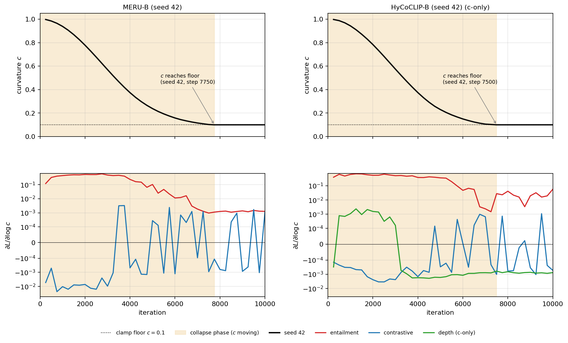
This explains why the full objective favors the low-curvature basin. Entailment cones have aperture \[\omega(\rho) = \arcsin\!\left( \min\!\left\{ 1,\; \frac{2K}{\sqrt{c}\,\rho} \right\} \right).\] As foreshadowed in Section 5.2, reducing \(c\) widens the aperture, which reduces violations in the training (text\(\to\)image) direction—realized jointly with norm compression—without requiring semantic hierarchy to be learned. Thus the hierarchy-motivated entailment objective contains a low-curvature, wide-cone shortcut, and the gradient decomposition in Figure 4 confirms that during collapse the entailment term drives \(c\) downward by a magnitude that exceeds the contrastive gradient on this full-objective trajectory, with the c-down sign pattern preserved under objective weighting.
This shortcut is self-limiting, which explains why, in the clampOff runs, curvature settles above the relaxed \(0.001\) clamp rather than running to it. The entailment c-down pressure is generated by violated pairs. Its magnitude is non-monotonic over training: it rises to a peak as curvature falls and violations are most active, then falls once apertures saturate and fewer pairs violate the cone constraint. During the collapse phase, on this full-objective trajectory, the measured contrastive gradient runs counter to this descent while it carries signal—with smaller or comparable magnitude early and much smaller magnitude later. Once \(c\) is pinned at the floor, the contrastive gradient is at noise level with no stable sign and should not be read as a persistent restoring force. The equilibrium is therefore consistent with a balance at the saturation edge: below it, apertures saturate and the entailment c-down pressure vanishes; above it, violations are active and entailment pushes \(c\) down. Whether this balance is a stable attractor—whether the c-down pressure just above the edge is steep enough to dominate the contrastive push—is a dynamical question we leave to future work. The analysis below establishes only where the saturation edge lies, and that curvature settles there rather than at the floor.
The location of this boundary follows in closed form. The half-aperture is \(\omega(\rho)=\arcsin\!\bigl(\min\{1,\,2K/(\sqrt{c}\,\rho)\}\bigr)\) with \(K\) the fixed constant in the aperture formula (\(K=0.1\) in all three audited implementations, including PHyCLIP’s per-factor cones; distinct from the curvature floor that coincidentally also equals \(0.1\) at baseline), so a cone saturates (\(\omega=\pi/2\)) exactly when \(\sqrt{c}\,\rho \le 2K = 0.2\). The clampOff equilibria land at this edge: with the floor relaxed to \(0.001\), HyCoCLIP-B settles at \(c\approx0.009\) with \(\rho\approx2.06\) (Table 14, measured on the same GRIT shards as the Table 4 cones), giving \(\sqrt{c}\,\rho\approx0.195 < 0.2\), i.e.apertures at saturation, matching the saturated cones of Section 5.2. The same holds across all audited clampOff cases: HyCoCLIP-B and HyCoCLIP-S (both \(\sqrt{c}\rho\approx0.195\)), MERU-B (\(0.178\)–\(0.182\) across seeds), and PHyCLIP-S and PHyCLIP-B (\(0.188\))2 all sit below \(2K\) with median apertures observed at \(\pi/2\) (image-side saturation \(95.6\%\) for PHyCLIP-B, \(95.5\%\) for PHyCLIP-S, \(\geq99\%\) for the others), as the aperture identity requires. MERU-S (\(0.217 > 0.2\), single seed) sits above the edge and its image-side cone remains non-saturated (\(1.175\) rad, Table 4), consistent with the identity. Because the half-aperture is a monotone function of \(\sqrt{c}\rho\), that a run at \(\sqrt{c}\rho<0.2\) has saturated cones is an identity, not an independent prediction. The empirical, falsifiable content is where the equilibria land. That every audited clampOff run—across families with opposite baseline cone regimes, and including the non-saturated MERU-S case—settles at or near the \(2K\) edge (from both sides) rather than at the relaxed \(0.001\) floor is strong evidence that the equilibrium is set by aperture saturation rather than by the clamp.
Three further observations sharpen this. First, the entailment objective creates an equilibrium at the edge wherever the edge is reachable: already under the \(0.1\) floor at \(500\)k steps, the HyCoCLIP-B and PHyCLIP-B baselines sit at \(\sqrt{c}\rho=0.202\) and \(0.206\). Second, MERU-B baseline (\(0.297\)) is the clamp-pinned case: the \(c=0.1\) floor halts descent before \(\rho\) reaches the edge, and releasing the floor lets it continue to \({\approx}0.18\)—so the equilibrium is set by the edge when reachable and by the clamp when not. Third, without entailment no such arrest appears: all six \(\lambda_{\mathrm{e}}{=}0\) runs are still contracting at their probe horizons (\(\sqrt{c}\rho=0.33\)–\(0.35\) at \({\sim}11\)k steps, slopes \(-0.035\) to \(-0.048\) per \(1\)k steps), and the extended seed-0 runs in both families pass through the edge at \({\approx}21\)–\(22\)k and continue smoothly to \(0.103\)–\(0.106\) at \(40\)k with no inflection or arrest at \(0.2\) (Section 7.4). The \(\lambda_{\mathrm{e}}{=}0\) horizons (\(11\)–\(40\)k) and the clampOff endpoints (\(500\)k) are not a matched-horizon comparison. The contrast is between arrest at the edge and the absence of any stationary point, not between endpoint values. MERU-B clampOff is seed-consistent: across three seeds it settles at \(\sqrt{c}\rho=0.176\)–\(0.180<0.2\) with the image cone saturated, and all three seeds remain near-Euclidean (\(H(u)\approx1.005\); per-seed geometry in Table 15).
The informative fact is not that saturation tracks the identity—it must—but that every equilibrium lands within \(0.024\) of the edge itself. The collapse-phase gradients that drive \(c\) down are not in tension with this above-floor equilibrium: the saturation they produce is precisely what removes the entailment pressure as the equilibrium is reached. Tables 14 and 13 thus record the same fact in two coordinates: the curvature at which \(c\) stops places every run at or near the \(2K\) edge—just below it for the saturating runs, just above for the non-saturating ones.
The evidence for this shortcut is of three kinds, of decreasing independence from training noise. First, it is analytic: the aperture relation \(\omega(\rho)=\arcsin\!\bigl(2K/(\sqrt{c}\rho)\bigr)\) means that lowering curvature mechanically widens cones and suppresses violations, independent of any run. Second, it is an equilibrium-location match: across families with opposite baseline cone regimes—and seed-consistently in the MERU-B triplet—the clampOff equilibria settle at or near the \(2K\) aperture-saturation edge rather than at the relaxed \(0.001\) floor, while the entailment-off runs show no arrest there, contracting through the edge with no stationary point in either family (Section 7.4), so the arrest at the edge is specific to the entailment objective, not a per-run accident. (That saturation coincides with \(\sqrt{c}\rho\le2K\) is an aperture-formula identity, not an independent measurement.) Third, it is an empirical gradient probe: the per-loss decomposition on the full-objective collapse-probe trajectories shows the entailment term pushing curvature down and the contrastive term up, consistently across checkpoints and for MERU-B (no depth term), replicating across all three seeds (Appendix 16.2). The first two kinds of evidence carry the claim. The gradient signs corroborate the direction without being load-bearing for the conclusion.
It is worth stating plainly how this mechanism connects to the released checkpoints, since the two are established by different means. The causal demonstration—intervening on the curvature floor and reading off the resulting aperture and gradient behavior—is exercised only on the from-scratch current-GRIT clampOff runs, because the released checkpoints are all pinned at the floor and cannot themselves be intervened on. What bridges the two is not a second causal experiment but two seed- and corpus-independent facts: the from-scratch baselines converge to the same dimensionless operating point as the released checkpoints (\(\sqrt{c}\rho\approx0.2\)–\(0.3\), Section 4.1), and the saturation criterion \(\sqrt{c}\rho\le2K\) is parameter-free, so it applies to any checkpoint regardless of how it was trained. The released checkpoints occupy the same near-threshold, near-Euclidean operating regime, and the cone sides that the aperture identity implies are saturated are observed saturated (text-side cones uniformly at \(\pi/2\); image-side cones sit at the edge, since released image \(\sqrt{c}\rho\) is at or just above \(0.2\)). The clampOff runs let us watch the objective drive a model to that boundary. The mechanistic account of why curvature collapses is thus validated interventionally on the current-GRIT runs and connected to the released artifacts through the shared, parameter-free operating-point criterion rather than through a claim that the released checkpoints were themselves intervened on.
The depth term faces a difficulty in either direction. When the active-pair radial ordering is partially correct (\(\rho_{\mathrm{child}} > \rho_{\mathrm{parent}}\) for the majority of active pairs), the depth gradient is c-up but small in magnitude (Table 37). When the radial ordering is wrong-signed or absent, the depth term flips to c-down and contributes nothing positive. In either regime, allowing radii to update through the depth term reopens the norm-growth path (Section 7.2). Successful objectives must therefore jointly learn radial ordering, identify curvature, and control radial growth—three requirements the audited objectives do not satisfy together.
The shortcut identified here dominates curvature descent on the full objective, but the next section shows it is not the only route to low curvature: removing the entailment term entirely still fails to preserve a nonlocal operating point (Section 7.4)—entailment is the dominant accelerator, not a necessary cause.
7.4 Entailment-off training does not stabilize curvature↩︎
The gradient decomposition attributes the dominant curvature-lowering pressure to the entailment term on the full-objective trajectory. A natural question is whether that term is also necessary for collapse: if the cone loss is the cause, removing it should leave curvature high. We test this directly by setting the entailment weight to zero (\(\lambda_{\mathrm{e}}{=}0\)) and retraining from scratch as otherwise-matched current-GRIT collapse probes (\({\sim}11\)k steps; seed 0 extended to \(40\)k in both families; per-variant horizons in Appendix 11), for both ViT-B families across three seeds (\(0/37/42\)). For MERU-B this leaves a contrastive-only objective; for HyCoCLIP-B it is an entailment-off objective retaining the box-level compositional and non-entailment alignment terms.
Removing entailment does not stabilize curvature (Figure 5, Table 6). In every run curvature still collapses to the clamp floor and the operating point keeps contracting through the probe horizon (below). This is consistent with the full-objective gradient decomposition (Figure 4): the contrastive c-up gradient there carries signal only transiently and is not a persistent restoring force, so once it decays nothing holds curvature up. Entailment is not necessary for collapse in these settings. What it supplies is a substantial acceleration of it: with the cone loss active (\(\lambda_{\mathrm{e}}{=}0.2\)) curvature reaches the floor roughly \(2600\)–\(2800\) steps earlier than without it (floor at \({\sim}7.3\)–\(7.5\)k vs. \({\sim}9.8\)–\(10.3\)k), consistent across families and seeds at matched clamp and protocol (not seed-paired—Table 6).

| Model | \(\lambda_{\mathrm{e}}\) | floor step | \(c@3\)k | \(c@5\)k | \(c@7\)k |
|---|---|---|---|---|---|
| MERU-B | \(0.2\) | \(7500\) | \(0.570\) | \(0.237\) | \(0.115\) |
| MERU-B | \(0\) | \(10233\) | \(0.761\) | \(0.423\) | \(0.237\) |
| HyCoCLIP-B | \(0.2\) | \(7250\) | \(0.575\) | \(0.230\) | \(0.107\) |
| HyCoCLIP-B | \(0\) | \(9833\) | \(0.766\) | \(0.422\) | \(0.230\) |
The entailment-off runs also expose what the non-entailment objective does on its own. Early in training \(\sqrt{c}\rho\) transiently overshoots into the nonlocal regime (Figure 5, bottom; peak \(\approx1.6\)–\(1.7\) at step \({\sim}1.3\)–\(1.8\)k; \(\sqrt{c}\rho>1\), both families, all seeds)3 and then contracts as both \(c\) and \(\rho\) fall: at the \({\sim}11\)k probe horizon all six runs sit at \(\sqrt{c}\rho=0.33\)–\(0.35\) with terminal slopes of \(-0.035\) to \(-0.048\) per \(1\)k steps—still contracting, the endpoints transient rather than stationary. Extended to \(40\)k (seed 0, both families)4, the runs pass through the \(2K{=}0.2\) edge at \({\approx}21\)–\(22\)k and decline smoothly to \(0.106\) (MERU-B) and \(0.103\) (HyCoCLIP-B) at \(40\)k with no stationary point—the edge is a reference landmark only here, since without the cone term it has no dynamical role for these runs. Once \(c\) is pinned at the floor, this continued contraction is entirely \(\rho\)-side. The objective thus reaches the nonlocal operating point its geometry is built for but does not hold it—unlike the entailment-on clampOff arrest at the edge (\(0.18\)–\(0.22\) at \(500\)k; Section 7.3): absent a curvature-identifying signal, contrastive alignment leaves curvature underidentified and the operating point contracts. EuCLIP’s sweep already includes entailment-free hyperbolic runs whose scalar curvature likewise ends at the clamp floor [13]. The operating-point trajectory is what that endpoint conceals—the overshoot, the contraction without a stationary point, and the absence of any arrest at the \(2K\) edge.
Two caveats bound this picture. First, the curvature collapse is not a weight-decay artifact—the learned curvature is excluded from weight decay—and the \(\lambda_{\mathrm{e}}{=}0\) gradient probe shows a weak but predominantly downward contrastive curvature gradient through the collapse phase, so the descent is driven rather than a passive drift. The contrastive gradient’s sign is thus trajectory-dependent—c-up on the full objective (Figure 4), predominantly c-down once entailment is removed. Second, the accompanying radial-norm contraction is not cleanly attributable to the objective: the shared recipe applies weight decay (\(0.2\)) to the encoder, which shrinks \(\rho\)—and hence \(\sqrt{c}\rho\)—after the warmup transient, so weight decay and the logit temperature remain unruled confounds for the norm side of the contraction. A weight-decay-reduced run would isolate this. The ablation’s load-bearing conclusion—that the non-entailment objective does not hold curvature high or pin a nonlocal operating point—does not depend on that isolation.
The two failures are therefore separable and asymmetric. Contrastive/alignment underidentification supplies only a weak, unstable pressure that fails to stabilize a nonlocal operating point. The entailment shortcut adds a much stronger aperture-driven descent that accelerates collapse. Entailment is the dominant accelerator on the full-objective trajectory, not the sole possible route to low curvature—which is why a future model must fix the contrastive/alignment objective (Section 7.5, item 2), not merely the entailment loss.
7.5 Design requirements for future hyperbolic VLMs↩︎
None of these failures shows that hyperbolic geometry is the wrong tool for vision-language learning. What they pin down is why current published formulations leave the radial/cone mechanism dormant, and what a future model would have to demonstrate to claim otherwise.
A hyperbolic VLM claiming hierarchy should report at least the following diagnostics:
Nonlocal geometry activation: learned curvature, radial norms, \(\sqrt{c}\rho\) distributions, local distortion factors, and the fraction of embeddings in the nonlocal regime.
Curvature identifiability: whether curvature gradients come from contrastive, entailment, or hierarchy losses, and whether curvature can change without being absorbed by radial norm scale. In particular, whether contrastive alignment stabilizes a nonlocal operating point rather than letting \(\sqrt{c}\rho\) contract toward the Euclidean basin (Section 7.4).
Active entailment: cone aperture distributions, active violation rates, containment of true directed pairs, evidence that zero violation is not due to saturated apertures, and whether the order objective can be satisfied without lowering \(c\), shrinking parent radii, or saturating apertures.
Directed hierarchy: parent-child radial ordering evaluated against shuffle-null controls and prompt-length confounds.
Operational hierarchy: traversal monotonicity, collapse rate, and terminal retrieval diversity.
Evaluation decomposition: separation of angular semantic organization from radial hierarchy in taxonomy-distance or hierarchy-aware metrics.
We distill this contract into a report format that authors and reviewers can adopt directly:
These are necessary-condition tests, not a complete benchmark for all hierarchy representations: a model may improve angular organization, stabilize cross-modal alignment, or reduce entailment violations without using active radial or cone-based hierarchy. Jointly, however, the criteria are far more constraining than any single test: a model that activates nonlocal geometry, identifies curvature independently of radial scale, maintains active and contained cones, and passes the directed and operational tests has closed each escape route by which the audited models pass the diagnostics they do pass. Passing all of them would still not prove the mechanism active—hierarchy could be realized in some form none of these tests detects—but a model reporting all of them gives readers the information needed to judge: the contract specifies what a hierarchy claim should report.
One might object that the audit is self-sealing: if our mechanism (Section 7.3) explains why no model leaves the near-Euclidean basin, then a negative hierarchy result is guaranteed by construction rather than measured. Two features of the design rule this out. First, the diagnostics are not blind to a positive: the graded positive controls (Appendix 14.1 and the planted-tree control of Appendix 14) show that the directed and taxonomy tests do fire when a pair-specific radial ordering is present, and collapse to chance only under the shuffle null—so a model that did instantiate the mechanism would register on them. Second, the non-detections are bounded, not open-ended: the MDE analysis quantifies the smallest shuffle-controlled signal we would have caught (\(\Delta_{\mathrm{pair}}\approx13\)pp for the radial test, \(\Delta R^2_{\mathrm{norm}}\approx0.013\) for the taxonomy test), and the audited hyperbolic and box-trained models’ shuffle-controlled excesses fall well below that threshold (largest \(\approx5\)pp vs.the \(\approx13\)pp radial MDE; largest taxonomy increment \(\Delta R^2_{\mathrm{norm}}\leq0.0029\) vs.the \(0.013\) taxonomy MDE), so the null readings are bounded absences, not failures to look. The negative is therefore a measured absence within a quantified sensitivity envelope, on diagnostics demonstrated to detect the signal when it exists—not an artifact of restricting attention to a regime where the signal cannot appear. That the models do not reach the nonlinear regime is itself one of our findings (Section 4), with a mechanistic account of why. It is a property of the audited objectives, not an assumption built into the tests.
8 Conclusion↩︎
We asked whether public hyperbolic vision–language models use the geometry they are built around, and found two distinct, separable failures. First, curvature is not an active geometric resource in any audited configuration: across MERU, HyCoCLIP, and PHyCLIP—released and trained from scratch—the dimensionless operating point stays near-Euclidean (\(\sqrt{c}\rho\approx0.2\)–\(0.3\), \(H(u)\approx1\), no evaluated checkpoint in the nonlocal regime), and releasing the curvature floor moves scalar curvature and norms while the operating point stays in the near-Euclidean band. Second, the cone and traversal machinery is measured inoperative—apertures saturated or misaligned, graded traversal failing under controlled readouts—while directed radial depth is a bounded non-detection: external parent–child ordering shows no signal above shuffle-null controls at quantified sensitivity, leaving only a tiny, non-operative residual on the models’ own native relation. A gradient-level mechanism explains why the natural interventions do not repair this—the entailment objective itself admits a low-curvature, wide-cone shortcut, and under a parameter-free aperture relation (\(\sqrt{c}\rho\le2K\)) curvature settles at the aperture-saturation edge in every entailment-trained unclamped run. Entailment-off ablations further show that fixing the cone loss alone would be insufficient: contrastive/alignment training also fails to hold curvature up (the norm side of the contraction is confounded with weight decay), though the entailment shortcut is the dominant full-objective accelerator.
These results do not show that hyperbolic geometry is the wrong tool for vision–language learning. They show that current published formulations leave its mechanism dormant, and that the evidence usually read as hierarchy is carried by angular structure or box/compositional supervision effects rather than radial depth. To make future claims checkable rather than assumed, we distill our diagnostics into a five-number geometry report (Section 7.5)—operating point, cone-saturation state, directed violations, shuffle-controlled radial excess, and radial increment beyond angle—paired with the operational-hierarchy traversal statistics. A model that reports these lets readers judge whether its geometry is active, not merely present.
Reproducibility Statement↩︎
We release the full audit suite as supplementary material (Appendix 17): measurement scripts, the raw per-run outputs behind every table, checkpoint SHA-256 hashes, current-GRIT training configurations, and the radius/curvature/aperture convention documents. The released MERU, HyCoCLIP, and PHyCLIP checkpoints are identified by their hashes; the from-scratch current-GRIT checkpoints are available on request and will be released publicly on publication. Every reported table can be re-derived from the persisted outputs alone—the weights and configurations are needed only to regenerate those outputs from scratch.
9 Notation↩︎
Table 7 collects the symbols used throughout the paper.
| Symbol | Meaning |
|---|---|
| \(c\) | Learned curvature parameter. |
| \(\rho = \lVert x \rVert\) | Radial coordinate: the Lorentz spatial norm (distance from the origin). |
| \(u = \sqrt{c}\,\rho\) | Dimensionless operating point. |
| \(\sqrt{c}\rho > 1\) | Marker for the nonlocal (operative-hyperbolic) regime. |
| \(H(u) = \sinh(u)/u\) | Local distortion factor; \(H \approx 1\) is near-Euclidean and grows in the nonlocal regime. |
| \(K\) | Fixed constant in the cone-aperture formula (\(K = 0.1\)); a cone saturates when \(\sqrt{c}\rho \le 2K\). |
| \(\omega(\rho)\) | Entailment-cone half-aperture. |
| \(R^2_{\cos}\) | Taxonomy-distance variance explained by cosine (angular) distance. |
| \(\Delta R^2_{\mathrm{norm}}\) | Incremental \(R^2\) of embedding norm beyond cosine distance. |
| \(z\) | Shuffle-null standardized score (directed radial test). |
| \(\Delta_{\mathrm{pair}}\) | Shuffle-controlled pair-specific excess (radial ordering). |
| \(p_{\mathrm{perm}}\) | Mantel / shuffle permutation-test \(p\)-value. |
| \(\eta\) | Entailment activation threshold. |
| NG2 | The model-native GRIT box\(\to\)full-caption relation (its own training relation). |
10 Full Geometry Diagnostics↩︎
10.1 Released-checkpoint per-modality local distortion↩︎
| Model | Modality | \(c\) | \(\rho\) | \(\sqrt{c}\rho\) | \(H(u)\) |
|---|---|---|---|---|---|
| MERU-S | image | 0.100 | 0.816 | 0.258 | 1.0111 |
| MERU-S | text | 0.100 | 0.547 | 0.173 | 1.0050 |
| MERU-B | image | 0.100 | 0.834 | 0.264 | 1.0116 |
| MERU-B | text | 0.100 | 0.578 | 0.183 | 1.0056 |
| MERU-L | image | 0.100 | 0.882 | 0.279 | 1.0130 |
| MERU-L | text | 0.100 | 0.599 | 0.190 | 1.0060 |
| HyCoCLIP-S | full image | 0.100 | 0.635 | 0.201 | 1.0067 |
| HyCoCLIP-S | box image | 0.100 | 0.630 | 0.199 | 1.0066 |
| HyCoCLIP-S | full text | 0.100 | 0.389 | 0.123 | 1.0025 |
| HyCoCLIP-S | box text | 0.100 | 0.319 | 0.101 | 1.0017 |
| HyCoCLIP-B | full image | 0.100 | 0.636 | 0.201 | 1.0068 |
| HyCoCLIP-B | box image | 0.100 | 0.630 | 0.199 | 1.0066 |
| HyCoCLIP-B | full text | 0.100 | 0.385 | 0.122 | 1.0025 |
| HyCoCLIP-B | box text | 0.100 | 0.324 | 0.102 | 1.0018 |
| PHyCLIP-B | full image | 0.100\(^\dagger\) | 0.681 | 0.215 | 1.0078 |
| PHyCLIP-B | box image | 0.100\(^\dagger\) | 0.647 | 0.205 | 1.0071 |
| PHyCLIP-B | full text | 0.100\(^\dagger\) | 0.442 | 0.140 | 1.0033 |
| PHyCLIP-B | box text | 0.100\(^\dagger\) | 0.365 | 0.115 | 1.0023 |
| PHyCLIP-L | full image | 0.100\(^\dagger\) | 0.690 | 0.218 | 1.0080 |
| PHyCLIP-L | box image | 0.100\(^\dagger\) | 0.652 | 0.206 | 1.0072 |
| PHyCLIP-L | full text | 0.100\(^\dagger\) | 0.442 | 0.140 | 1.0033 |
| PHyCLIP-L | box text | 0.100\(^\dagger\) | 0.370 | 0.117 | 1.0024 |
10.2 Operating-point upper tail: \(\sqrt{c}\rho\) quantiles↩︎
Tables 1 and 2 report median/mean \(\sqrt{c}\rho\) and the nonlocal-regime fraction (\(\sqrt{c}\rho>1\)). To rule out rare high-radius samples a median could hide, Table 9 adds the upper tail—\(95\)th/\(99\)th percentiles and maximum—of the per-sample image-side \(\sqrt{c}\rho\) for every audited checkpoint. Across every audited checkpoint (over \(500\) ImageNet val images), the largest single \(\sqrt{c}\rho\) is \(0.367\) (released PHyCLIP-B). Local distortion \(H(u)\) reaches \(10\%\) only at \(\sqrt{c}\rho\approx0.76\), and the nonlocal regime only at \(\sqrt{c}\rho=1\) (Section 3, Figure 1). The observed maximum is below half the former and just over a third of the latter. PHyCLIP’s wider tail reflects its widest subspace.
| Model | Setting | Seed | median | p95 | p99 | max |
|---|---|---|---|---|---|---|
| MERU-S | released | — | 0.258 | 0.264 | 0.267 | 0.269 |
| MERU-B | released | — | 0.264 | 0.270 | 0.273 | 0.278 |
| MERU-L | released | — | 0.279 | 0.287 | 0.290 | 0.292 |
| HyCoCLIP-S | released | — | 0.200 | 0.203 | 0.204 | 0.205 |
| HyCoCLIP-B | released | — | 0.201 | 0.204 | 0.205 | 0.206 |
| PHyCLIP-B | released | — | 0.213 | 0.257 | 0.279 | 0.367 |
| PHyCLIP-L | released | — | 0.216 | 0.262 | 0.287 | 0.351 |
| MERU-S | baseline | 0 | 0.291 | 0.299 | 0.302 | 0.306 |
| MERU-B | baseline | 0 | 0.296 | 0.305 | 0.308 | 0.310 |
| HyCoCLIP-S | baseline | 0 | 0.201 | 0.203 | 0.204 | 0.207 |
| HyCoCLIP-B | baseline | 0 | 0.201 | 0.203 | 0.204 | 0.205 |
| PHyCLIP-S | baseline | 0 | 0.202 | 0.239 | 0.257 | 0.317 |
| PHyCLIP-B | baseline | 0 | 0.204 | 0.242 | 0.263 | 0.314 |
| MERU-S | clampOff | 0 | 0.216 | 0.221 | 0.224 | 0.224 |
| HyCoCLIP-S | clampOff | 0 | 0.194 | 0.197 | 0.197 | 0.198 |
| PHyCLIP-S | clampOff | 0 | 0.187 | 0.199 | 0.205 | 0.222 |
| MERU-B | clampOff | 0 | 0.180 | 0.185 | 0.187 | 0.189 |
| MERU-B | clampOff | 37 | 0.177 | 0.181 | 0.183 | 0.184 |
| MERU-B | clampOff | 42 | 0.179 | 0.184 | 0.186 | 0.187 |
| HyCoCLIP-B | clampOff | 0 | 0.195 | 0.197 | 0.198 | 0.199 |
| HyCoCLIP-B | clampOff | 37 | 0.194 | 0.197 | 0.197 | 0.198 |
| HyCoCLIP-B | clampOff | 42 | 0.195 | 0.197 | 0.197 | 0.198 |
| PHyCLIP-B | clampOff | 0 | 0.187 | 0.200 | 0.206 | 0.225 |
| PHyCLIP-B | clampOff | 37 | 0.187 | 0.199 | 0.206 | 0.225 |
| PHyCLIP-B | clampOff | 42 | 0.187 | 0.200 | 0.206 | 0.229 |
10.3 Full per-seed downstream and evaluation results↩︎
This section is reproducibility material: the complete per-seed absolute metrics underlying Table 3 (full precision, seeds \(0/37/42\), baseline and clampOff), from which each reported delta can be recomputed directly. Tables 10, 11, and 12 cover retrieval and WordNet hierarchical metrics, the \(16\)-task zero-shot suite, and the per-subtype compositional results, respectively. Across all metrics and models, curvature unclamping produces only small, seed-comparable shifts with no substantial degradation.
| Text\(\to\)Image | Image\(\to\)Text | Hierarchical Classification | ||||||||||||
|---|---|---|---|---|---|---|---|---|---|---|---|---|---|---|
| 3-6(lr)7-10(lr)11-15 | COCO | Flickr | COCO | Flickr | WordNet | |||||||||
| 3-4(lr)5-6(lr)7-8(lr)9-10(lr)11-15 Model / setting | seed | R@5 | R@10 | R@5 | R@10 | R@5 | R@10 | R@5 | R@10 | TIE\(\downarrow\) | LCA\(\downarrow\) | J\(\uparrow\) | PH\(\uparrow\) | RH\(\uparrow\) |
| MERU-B baseline | 0 | 55.28 | 66.40 | 81.38 | 88.28 | 68.52 | 78.82 | 89.10 | 94.60 | 3.872 | 2.330 | 0.7707 | 0.8426 | 0.8440 |
| 37 | 55.75 | 67.27 | 82.08 | 88.66 | 69.84 | 79.76 | 90.10 | 94.90 | 3.903 | 2.331 | 0.7685 | 0.8413 | 0.8417 | |
| 42 | 55.09 | 66.49 | 81.66 | 88.72 | 68.58 | 78.34 | 90.40 | 94.80 | 3.864 | 2.307 | 0.7710 | 0.8438 | 0.8424 | |
| MERU-B clampOff | 0 | 55.50 | 66.99 | 81.48 | 88.22 | 68.28 | 79.12 | 88.80 | 94.30 | 3.886 | 2.313 | 0.7687 | 0.8428 | 0.8410 |
| 37 | 55.15 | 66.77 | 81.84 | 88.60 | 69.14 | 79.00 | 91.10 | 95.40 | 3.994 | 2.352 | 0.7618 | 0.8378 | 0.8355 | |
| 42 | 55.34 | 66.56 | 81.64 | 88.80 | 68.12 | 78.40 | 89.70 | 94.00 | 3.907 | 2.325 | 0.7682 | 0.8422 | 0.8409 | |
| HyCoCLIP-B baseline | 0 | 57.38 | 68.39 | 82.94 | 89.70 | 69.36 | 79.50 | 91.40 | 96.30 | 3.299 | 2.086 | 0.8054 | 0.8684 | 0.8670 |
| 37 | 56.31 | 67.28 | 82.60 | 89.54 | 69.34 | 79.74 | 90.50 | 95.10 | 3.395 | 2.125 | 0.8002 | 0.8642 | 0.8640 | |
| 42 | 57.33 | 68.40 | 83.50 | 89.96 | 70.44 | 80.38 | 91.80 | 95.80 | 3.282 | 2.077 | 0.8070 | 0.8692 | 0.8687 | |
| HyCoCLIP-B clampOff | 0 | 57.64 | 69.07 | 84.12 | 90.28 | 71.40 | 80.68 | 92.30 | 95.40 | 3.353 | 2.083 | 0.8017 | 0.8673 | 0.8627 |
| 37 | 57.44 | 68.69 | 83.16 | 89.84 | 70.92 | 80.98 | 92.10 | 96.70 | 3.498 | 2.173 | 0.7947 | 0.8599 | 0.8590 | |
| 42 | 58.82 | 69.53 | 83.92 | 90.74 | 71.62 | 81.00 | 92.30 | 95.30 | 3.378 | 2.118 | 0.8002 | 0.8647 | 0.8620 | |
| PHyCLIP-B baseline | 0 | 56.84 | 68.18 | 82.92 | 89.78 | 69.94 | 79.96 | 91.70 | 95.40 | 3.346 | 2.111 | 0.8034 | 0.8665 | 0.8661 |
| 37 | 57.01 | 67.95 | 82.60 | 89.28 | 70.56 | 79.56 | 90.80 | 95.10 | 3.342 | 2.124 | 0.8042 | 0.8659 | 0.8677 | |
| 42 | 56.79 | 68.13 | 82.96 | 89.46 | 69.64 | 79.76 | 90.60 | 94.80 | 3.284 | 2.070 | 0.8067 | 0.8697 | 0.8671 | |
| PHyCLIP-B clampOff | 0 | 57.34 | 68.41 | 83.64 | 89.98 | 70.98 | 80.50 | 91.20 | 95.60 | 3.375 | 2.106 | 0.8009 | 0.8655 | 0.8629 |
| 37 | 57.54 | 68.76 | 82.64 | 89.34 | 70.66 | 80.16 | 91.00 | 95.40 | 3.377 | 2.110 | 0.8002 | 0.8650 | 0.8627 | |
| 42 | 57.68 | 68.53 | 83.50 | 90.08 | 70.40 | 80.34 | 91.40 | 95.70 | 3.367 | 2.097 | 0.8010 | 0.8660 | 0.8632 | |
3pt
| Model / setting | seed | IN | C10 | C100 | SUN | Cal | STL | Food | CUB | Cars | Airc | Pets | Flwr | DTD | Euro | RES | C211 |
|---|---|---|---|---|---|---|---|---|---|---|---|---|---|---|---|---|---|
| MERU-B baseline | 0 | 37.32 | 75.31 | 45.11 | 49.45 | 72.24 | 92.80 | 48.89 | 8.44 | 7.22 | 2.42 | 42.40 | 17.78 | 20.59 | 37.14 | 40.36 | 5.05 |
| 37 | 37.06 | 73.96 | 42.79 | 50.30 | 72.37 | 93.50 | 49.64 | 10.73 | 6.84 | 2.15 | 41.74 | 21.62 | 22.93 | 40.90 | 41.36 | 4.36 | |
| 42 | 37.39 | 75.28 | 44.00 | 50.05 | 73.25 | 92.55 | 47.90 | 9.44 | 7.07 | 2.33 | 40.43 | 15.09 | 19.84 | 37.82 | 41.41 | 4.91 | |
| MERU-B clampOff | 0 | 37.12 | 70.66 | 44.21 | 49.41 | 72.49 | 93.39 | 46.44 | 11.12 | 6.96 | 2.36 | 41.47 | 17.28 | 22.23 | 34.67 | 37.52 | 4.75 |
| 37 | 36.40 | 74.14 | 44.03 | 49.58 | 72.08 | 93.19 | 47.03 | 10.54 | 6.21 | 2.36 | 43.42 | 20.85 | 19.31 | 40.89 | 43.67 | 4.54 | |
| 42 | 36.87 | 76.02 | 43.21 | 49.86 | 71.76 | 92.66 | 50.58 | 10.43 | 6.43 | 2.09 | 44.79 | 16.58 | 21.33 | 47.27 | 42.21 | 4.72 | |
| HyCoCLIP-B baseline | 0 | 44.39 | 89.01 | 59.42 | 55.08 | 74.36 | 94.94 | 55.21 | 15.60 | 10.20 | 3.98 | 52.38 | 22.17 | 26.76 | 41.14 | 43.32 | 5.57 |
| 37 | 42.53 | 87.94 | 58.63 | 54.44 | 77.43 | 94.12 | 56.57 | 17.59 | 9.11 | 3.86 | 51.01 | 24.56 | 25.80 | 41.80 | 46.98 | 5.45 | |
| 42 | 44.06 | 89.04 | 59.27 | 55.04 | 76.93 | 95.06 | 59.65 | 18.37 | 9.80 | 3.28 | 53.28 | 26.06 | 24.84 | 39.89 | 49.62 | 5.81 | |
| HyCoCLIP-B clampOff | 0 | 43.71 | 87.84 | 57.11 | 54.47 | 75.80 | 94.33 | 57.46 | 16.29 | 10.64 | 3.09 | 51.83 | 26.39 | 26.38 | 42.13 | 42.92 | 5.98 |
| 37 | 42.38 | 88.26 | 57.93 | 54.09 | 75.22 | 93.82 | 55.14 | 15.63 | 10.08 | 3.56 | 49.77 | 24.97 | 22.98 | 32.28 | 44.28 | 5.92 | |
| 42 | 43.83 | 88.66 | 59.20 | 54.32 | 76.56 | 94.16 | 55.67 | 14.27 | 11.01 | 3.99 | 52.02 | 26.80 | 27.07 | 40.70 | 45.60 | 5.41 | |
| PHyCLIP-B baseline | 0 | 43.38 | 88.68 | 59.48 | 55.41 | 77.69 | 94.10 | 58.72 | 16.19 | 9.67 | 3.63 | 53.00 | 25.36 | 25.90 | 41.59 | 46.92 | 5.36 |
| 37 | 43.63 | 88.16 | 58.45 | 55.28 | 75.07 | 95.10 | 58.51 | 17.79 | 10.29 | 3.16 | 52.68 | 23.81 | 27.93 | 47.18 | 45.27 | 5.60 | |
| 42 | 44.25 | 88.70 | 60.74 | 55.92 | 77.31 | 95.19 | 59.20 | 15.86 | 10.55 | 3.17 | 52.99 | 25.29 | 27.61 | 40.17 | 48.66 | 5.63 | |
| PHyCLIP-B clampOff | 0 | 43.56 | 88.17 | 58.90 | 55.14 | 76.45 | 93.99 | 55.10 | 14.64 | 9.21 | 4.23 | 54.13 | 24.26 | 25.64 | 38.01 | 46.24 | 5.37 |
| 37 | 43.55 | 87.08 | 58.18 | 54.50 | 75.67 | 94.94 | 55.90 | 14.69 | 9.26 | 3.45 | 50.82 | 26.25 | 26.17 | 39.39 | 45.19 | 5.68 | |
| 42 | 43.27 | 88.16 | 58.34 | 53.77 | 77.67 | 95.00 | 57.40 | 15.47 | 10.59 | 2.75 | 50.40 | 23.35 | 27.18 | 41.87 | 46.45 | 5.73 |
3pt
| VL-CheckList-Object | SugarCrepe | ||||||||||||||
|---|---|---|---|---|---|---|---|---|---|---|---|---|---|---|---|
| 3-8(lr)9-16 Model / setting | seed | Loc-C | Loc-M | Loc-Mg | Sz-L | Sz-M | Sz-S | Rep-O | Rep-A | Rep-R | Swp-O | Swp-A | Add-O | Add-A | SC-All |
| MERU-B baseline | 0 | 62.90 | 60.30 | 61.60 | 64.00 | 60.60 | 58.80 | 90.68 | 79.57 | 69.84 | 57.14 | 63.96 | 80.02 | 71.68 | 77.47 |
| 37 | 62.10 | 58.10 | 57.10 | 62.90 | 57.60 | 55.50 | 88.92 | 81.09 | 69.77 | 60.82 | 66.52 | 80.80 | 72.69 | 77.89 | |
| 42 | 54.40 | 53.20 | 54.00 | 56.10 | 54.10 | 50.70 | 89.95 | 79.19 | 70.06 | 55.10 | 64.41 | 78.90 | 75.29 | 77.31 | |
| MERU-B clampOff | 0 | 60.80 | 60.50 | 61.80 | 63.40 | 61.10 | 55.20 | 89.53 | 79.95 | 69.20 | 57.96 | 67.42 | 80.21 | 72.83 | 77.63 |
| 37 | 64.60 | 62.80 | 61.00 | 65.30 | 62.50 | 59.30 | 89.65 | 79.57 | 69.49 | 60.41 | 67.72 | 81.96 | 71.10 | 78.10 | |
| 42 | 57.50 | 56.30 | 55.70 | 59.50 | 56.60 | 56.00 | 90.13 | 79.44 | 69.35 | 53.06 | 62.01 | 80.75 | 73.27 | 77.29 | |
| HyCoCLIP-B baseline | 0 | 67.50 | 68.10 | 69.30 | 69.60 | 65.00 | 66.40 | 90.80 | 77.66 | 65.79 | 58.37 | 64.41 | 82.06 | 73.41 | 77.34 |
| 37 | 75.00 | 74.30 | 70.90 | 75.70 | 71.00 | 71.20 | 91.16 | 80.71 | 65.58 | 58.78 | 64.56 | 81.57 | 70.81 | 77.35 | |
| 42 | 76.30 | 73.80 | 71.30 | 77.10 | 71.30 | 71.50 | 90.92 | 78.81 | 65.22 | 57.14 | 63.66 | 81.28 | 74.42 | 77.15 | |
| HyCoCLIP-B clampOff | 0 | 69.00 | 68.70 | 70.60 | 70.80 | 66.80 | 69.50 | 90.62 | 81.60 | 69.56 | 60.82 | 65.17 | 82.25 | 74.13 | 78.68 |
| 37 | 67.80 | 67.60 | 67.90 | 67.90 | 64.90 | 69.90 | 91.40 | 80.84 | 67.78 | 59.18 | 69.07 | 83.37 | 72.98 | 78.94 | |
| 42 | 69.80 | 68.70 | 68.00 | 70.90 | 65.20 | 68.10 | 90.86 | 81.60 | 67.85 | 53.06 | 65.17 | 83.27 | 72.69 | 78.31 | |
| PHyCLIP-B baseline | 0 | 76.60 | 73.00 | 73.10 | 76.70 | 70.70 | 72.00 | 91.10 | 80.33 | 65.50 | 60.41 | 64.86 | 81.09 | 74.42 | 77.57 |
| 37 | 73.30 | 70.80 | 68.80 | 73.80 | 67.70 | 66.90 | 90.98 | 80.33 | 66.64 | 60.82 | 66.52 | 82.10 | 70.09 | 77.79 | |
| 42 | 77.60 | 74.80 | 70.80 | 79.50 | 70.00 | 70.80 | 91.16 | 79.70 | 68.14 | 60.41 | 66.82 | 81.04 | 72.69 | 78.01 | |
| PHyCLIP-B clampOff | 0 | 78.20 | 75.80 | 75.10 | 77.80 | 75.00 | 74.30 | 90.74 | 82.11 | 68.92 | 60.41 | 65.77 | 83.75 | 74.86 | 79.16 |
| 37 | 76.20 | 72.60 | 71.70 | 75.90 | 70.70 | 71.20 | 91.16 | 80.20 | 67.71 | 59.18 | 62.91 | 83.46 | 75.00 | 78.47 | |
| 42 | 77.20 | 75.40 | 75.40 | 78.10 | 73.20 | 74.60 | 91.22 | 80.20 | 66.71 | 56.73 | 62.91 | 82.69 | 75.14 | 78.02 | |
3pt
10.4 Cone aperture and entailment violation diagnostics↩︎
Table 13 reports the full cone diagnostics across families, sizes, released checkpoints, and clampOff, for all three seeds. The patterns match Section 5.2: the i\(\to\)t rate is \(\approx100\%\) everywhere (text never enters the active image cone), and the small t\(\to\)i rate reflects embedding compression, not order. From opposite baseline image-cone regimes—MERU narrow (\(\approx 0.74\) rad), HyCoCLIP wide (\(\approx 1.45\) rad)—both families saturate to \(\pi/2\) under clampOff at ViT-B. The exception is MERU-S clampOff (\(0.75 \to 1.175\) rad, not fully saturated). In all cases the clampOff cone provides no operational hierarchy.
| Model | Setting | \(c\) | img aper (rad, sat%) | text aper (rad, sat%) | i\(\to\)t viol % | t\(\to\)i viol % | bt\(\to\)bi viol % |
|---|---|---|---|---|---|---|---|
| MERU-S | released\(^{\ddagger}\) | 0.100 | 0.875 (0%) | 1.571 (98.8%) | 100.0 | 48.4 | – |
| MERU-B | released\(^{\ddagger}\) | 0.100 | 0.852 (0%) | 1.571 (98.0%) | 100.0 | 64.8 | – |
| MERU-L | released\(^{\ddagger}\) | 0.100 | 0.802 (0%) | 1.571 (97.7%) | 100.0 | 70.7 | – |
| HyCoCLIP-S | released | 0.100 | 1.475 (30.5%) | 1.571 (100%) | 100.0 | 0.39 | 0.00 |
| HyCoCLIP-B | released | 0.100 | 1.456 (26.2%) | 1.571 (100%) | 100.0 | 0.39 | 0.00 |
| PHyCLIP-B | released | 0.100 | 1.219 (24.6%) | 1.569 (99.4%) | 100.0 | 8.5 | 6.3 |
| PHyCLIP-L | released | 0.100 | 1.185 (21.4%) | 1.569 (99.5%) | 100.0 | 6.3 | 5.4 |
| MERU-S | baseline | 0.100 | 0.751 (0%) | 1.571 (99.2%) | 100.0 | 5.1 | – |
| MERU-S | clampOff | 0.042 | 1.175 (0%) | 1.571 (100%) | 100.0 | 5.5 | – |
| MERU-B | baseline (s0) | 0.100 | 0.732 (0%) | 1.571 (99.6%) | 100.0 | 3.1 | – |
| MERU-B | baseline (s37) | 0.100 | 0.726 (0%) | 1.571 (99.2%) | 100.0 | 2.7 | – |
| MERU-B | baseline (s42) | 0.100 | 0.733 (0%) | 1.571 (99.2%) | 100.0 | 3.1 | – |
| MERU-B | clampOff (s0) | 0.029 | 1.571 (100%) | 1.571 (100%) | 100.0 | 1.6 | – |
| MERU-B | clampOff (s37) | 0.028 | 1.571 (100%) | 1.571 (100%) | 100.0 | 1.2 | – |
| MERU-B | clampOff (s42) | 0.029 | 1.571 (100%) | 1.571 (100%) | 100.0 | 3.1 | – |
| HyCoCLIP-S | baseline | 0.100 | 1.446 (15.6%) | 1.571 (100%) | 100.0 | 0.0 | 0.8 |
| HyCoCLIP-S | clampOff | 0.011 | 1.571 (100%) | 1.571 (100%) | 100.0 | 0.0 | 0.0 |
| HyCoCLIP-B | baseline (s0) | 0.100 | 1.422 (10.9%) | 1.571 (100%) | 100.0 | 0.0 | 0.0 |
| HyCoCLIP-B | baseline (s37) | 0.100 | 1.420 (12.9%) | 1.571 (100%) | 100.0 | 0.0 | 0.4 |
| HyCoCLIP-B | baseline (s42) | 0.100 | 1.423 (10.5%) | 1.571 (100%) | 100.0 | 0.4 | 0.4 |
| HyCoCLIP-B | clampOff (s0) | 0.009 | 1.571 (100%) | 1.571 (100%) | 100.0 | 0.0 | 0.0 |
| HyCoCLIP-B | clampOff (s37) | 0.009 | 1.571 (100%) | 1.571 (100%) | 100.0 | 0.0 | 0.0 |
| HyCoCLIP-B | clampOff (s42) | 0.009 | 1.571 (100%) | 1.571 (100%) | 100.0 | 0.0 | 0.0 |
| PHyCLIP-S | baseline | 0.100 | 1.417 (44.7%) | 1.571 (99.5%) | 100.0 | 13.8 | 6.5 |
| PHyCLIP-S | clampOff | 0.015 | 1.569 (95.5%) | 1.569 (100%) | 100.0 | 0.20 | 0.05 |
| PHyCLIP-B | baseline (s0) | 0.100 | 1.373 (41.7%) | 1.569 (99.7%) | 100.0 | 9.5 | 6.1 |
| PHyCLIP-B | baseline (s37) | 0.100 | 1.372 (40.9%) | 1.569 (99.7%) | 100.0 | 9.3 | 6.4 |
| PHyCLIP-B | baseline (s42) | 0.100 | 1.366 (41.4%) | 1.569 (99.7%) | 100.0 | 9.1 | 5.6 |
| PHyCLIP-B | clampOff (s0) | 0.014 | 1.569 (95.6%) | 1.569 (100%) | 100.0 | 0.05 | 0.04 |
| PHyCLIP-B | clampOff (s37) | 0.014 | 1.569 (95.5%) | 1.569 (100%) | 100.0 | 0.10 | 0.04 |
| PHyCLIP-B | clampOff (s42) | 0.015 | 1.569 (95.7%) | 1.569 (100%) | 100.0 | 0.09 | 0.05 |
10.5 Current-GRIT clampOff geometry by modality↩︎
| Model | Modality | \(c\) | \(\rho\) | \(\sqrt{c}\rho\) | \(H(u)\) |
|---|---|---|---|---|---|
| MERU-S baseline | image | 0.100 | 0.929 | 0.294 | 1.0145 |
| MERU-S baseline | text | 0.100 | 0.591 | 0.187 | 1.0059 |
| MERU-S clampOff | image | 0.042 | 1.061 | 0.217 | 1.0079 |
| MERU-S clampOff | text | 0.042 | 0.773 | 0.158 | 1.0042 |
| MERU-B baseline | image | 0.100 | 0.947 | 0.299 | 1.0150 |
| MERU-B baseline | text | 0.100 | 0.595 | 0.188 | 1.0059 |
| MERU-B clampOff | image | 0.029 | 1.060 | 0.182 | 1.0055 |
| MERU-B clampOff | text | 0.029 | 0.759 | 0.130 | 1.0028 |
| HyCoCLIP-S baseline | full image | 0.100 | 0.637 | 0.201 | 1.0068 |
| HyCoCLIP-S baseline | box image | 0.100 | 0.631 | 0.200 | 1.0067 |
| HyCoCLIP-S baseline | full text | 0.100 | 0.392 | 0.124 | 1.0026 |
| HyCoCLIP-S baseline | box text | 0.100 | 0.313 | 0.099 | 1.0016 |
| HyCoCLIP-S clampOff | full image | 0.011 | 1.848 | 0.195 | 1.0064 |
| HyCoCLIP-S clampOff | box image | 0.011 | 1.853 | 0.196 | 1.0064 |
| HyCoCLIP-S clampOff | full text | 0.011 | 1.350 | 0.143 | 1.0034 |
| HyCoCLIP-S clampOff | box text | 0.011 | 1.266 | 0.134 | 1.0030 |
| HyCoCLIP-B baseline | full image | 0.100 | 0.639 | 0.202 | 1.0068 |
| HyCoCLIP-B baseline | box image | 0.100 | 0.632 | 0.200 | 1.0067 |
| HyCoCLIP-B baseline | full text | 0.100 | 0.383 | 0.121 | 1.0024 |
| HyCoCLIP-B baseline | box text | 0.100 | 0.320 | 0.101 | 1.0017 |
| HyCoCLIP-B clampOff | full image | 0.009 | 2.058 | 0.195 | 1.0064 |
| HyCoCLIP-B clampOff | box image | 0.009 | 2.065 | 0.196 | 1.0064 |
| HyCoCLIP-B clampOff | full text | 0.009 | 1.515 | 0.144 | 1.0035 |
| HyCoCLIP-B clampOff | box text | 0.009 | 1.337 | 0.127 | 1.0027 |
| Model / setting | seed | \(c\) | \(\rho\) (img) | \(\sqrt{c}\rho\) | \(H(u)\) |
|---|---|---|---|---|---|
| MERU-S baseline | 0 | 0.1000 | 0.9206 | 0.2911 | 1.0142 |
| MERU-S clampOff | 0 | 0.0419 | 1.0523 | 0.2154 | 1.0078 |
| MERU-B baseline | 0 | 0.1000 | 0.9362 | 0.2961 | 1.0147 |
| 37 | 0.1000 | 0.9430 | 0.2982 | 1.0149 | |
| 42 | 0.1000 | 0.9371 | 0.2964 | 1.0147 | |
| MERU-B clampOff | 0 | 0.0294 | 1.0506 | 0.1800 | 1.0054 |
| 37 | 0.0281 | 1.0515 | 0.1762 | 1.0052 | |
| 42 | 0.0291 | 1.0451 | 0.1784 | 1.0053 | |
| HyCoCLIP-S baseline | 0 | 0.1000 | 0.6348 | 0.2007 | 1.0067 |
| HyCoCLIP-S clampOff | 0 | 0.0112 | 1.8390 | 0.1944 | 1.0063 |
| HyCoCLIP-B baseline | 0 | 0.1000 | 0.6379 | 0.2017 | 1.0068 |
| 37 | 0.1000 | 0.6377 | 0.2017 | 1.0068 | |
| 42 | 0.1000 | 0.6374 | 0.2016 | 1.0068 | |
| HyCoCLIP-B clampOff | 0 | 0.0090 | 2.0531 | 0.1949 | 1.0063 |
| 37 | 0.0094 | 2.0022 | 0.1945 | 1.0063 | |
| 42 | 0.0095 | 2.0017 | 0.1947 | 1.0063 | |
| PHyCLIP-S baseline | 0 | 0.1000 | 0.6440 | 0.2036 | 1.0070 |
| PHyCLIP-S clampOff | 0 | 0.0155 | 1.5084 | 0.1877 | 1.0059 |
| PHyCLIP-B baseline | 0 | 0.1000 | 0.6501 | 0.2056 | 1.0071 |
| 37 | 0.1000 | 0.6500 | 0.2055 | 1.0071 | |
| 42 | 0.1000 | 0.6507 | 0.2058 | 1.0071 | |
| PHyCLIP-B clampOff | 0 | 0.0143 | 1.5700 | 0.1876 | 1.0059 |
| 37 | 0.0144 | 1.5612 | 0.1874 | 1.0059 | |
| 42 | 0.0145 | 1.5539 | 0.1873 | 1.0059 |
5pt
10.6 PHyCLIP product-geometry convention↩︎
PHyCLIP uses a product-space implementation whose reported scalar curvature convention differs from the global-curvature convention used in MERU and HyCoCLIP. For this reason, PHyCLIP product-space diagnostics are reported factor-wise where applicable, and we avoid comparing a single scalar curvature across families unless the implementation convention is matched.
11 GRIT Snapshot and Training Details↩︎
11.1 Current-GRIT snapshot↩︎
| Quantity | Value |
|---|---|
| Download / crawl date | 2026-04-13 (file mtime) |
| Total shards (.tar) | 2,051 (all enumerated) |
| Processed corpus size | 731 GB |
| Image–text pairs | documented 20.5M / obtained \(13{,}064{,}747\) |
| Parent-box annotations | documented 35.9M / obtained \(25{,}018{,}042\) |
| Mean parent boxes per pair | 1.915 (\(25{,}018{,}042 / 13{,}064{,}747\)) |
| Pairs per shard | min 5,611, mean 6,370, max 6,540 |
| Effective epochs (training) | \({\approx}29\) (\(384\)M exposures \(/\) 13.06M pairs) |
| Mapper | GroundedDatasetTarMapper |
| Train image transform | RandomResizedCrop(224, scale=(0.5,1.0)) + ToTensor |
| Decoding failures | webdataset warn_and_continue |
A “parent-box annotation” is counted as one parent{NNN}.txt grounding entry per sample (the box_text source consumed by GroundedDatasetTarMapper), matching the per-sample box unit used elsewhere in this paper. The
documented \(35.9\)M figure is reproduced from the original release and may aggregate box annotations under a slightly different convention.
11.2 Training hyperparameters↩︎
| Family | Size | Variant | Curv. clamp | Changed variable |
|---|---|---|---|---|
| MERU | S/B | baseline | [0.1, 10] | none |
| MERU | S/B | clampOff | [0.001, 10] | curvature floor |
| MERU | B | \(\lambda_{\mathrm{e}}{=}0\) | [0.1, 10] | entailment weight (\(\to 0\)) |
| HyCoCLIP | S/B | baseline | [0.1, 10] | none |
| HyCoCLIP | S/B | clampOff | [0.001, 10] | curvature floor |
| HyCoCLIP | S/B | intra=\(0.7\) | [0.1, 10] | entailment threshold |
| HyCoCLIP | B | \(\lambda_{\mathrm{e}}{=}0\) | [0.1, 10] | entailment weight (\(\to 0\)) |
| PHyCLIP | S/B | baseline | [0.1, 10] | none |
| PHyCLIP | S/B | clampOff | [0.001, 10] | curvature floor |
The baseline and clampOff variants are matched on the same current-GRIT snapshot with global batch size \(768\), \(500{,}000\) iterations, AdamW (\(\mathrm{lr}=5\times10^{-4}\), \(\beta=(0.9,0.98)\), weight decay \(0.2\)), linear warmup (\(4000\) steps) followed by cosine
decay, no gradient accumulation (each iteration is a single optimizer step over \(768\) samples), and AMP enabled (fp16 forward, fp32 hyperbolic operations via explicit .float() casts in
phyclip/lorentz.py).5 Hardware was determined by model size: ViT-S variants were trained on a single H100, and all ViT-B runs (MERU, PHyCLIP, and HyCoCLIP) on
\(2\times\)H200. MERU-B clampOff seeds 37/42 were retrained on this unified \(2\times\)H200 setup after preliminary single-GPU runs showed hardware-dependent geometry. The retrained seeds
converge with seed 0. The global batch size of \(768\) was held fixed across all configurations and devices. ViT-L is not trained here. It is audited only at the released-checkpoint level (Table 8).
11.3 Threshold-activation stress test (\(\eta\) intervention)↩︎
This auxiliary single-seed intervention complements the entailment-off ablation of Section 7.4: rather than removing the entailment term, we activate it more strongly and find it likewise fails to install hierarchy.
Whereas the main-text interventions (Section 7) add or modify a curvature path, this stress test stays within the published objective, lowering the intra-modal entailment threshold \(\eta\) from the default \(1.2\) to \(0.7\). This is the most direct test of whether more active entailment cones induce hierarchy. We run it as a matched current-GRIT intervention on HyCoCLIP at both ViT-S and ViT-B (seed 0), changing only \(\eta\).
| ViT-B | ViT-S | |||||
|---|---|---|---|---|---|---|
| 2-4(lr)5-7 Quantity | \(\eta{=}1.2\) | \(\eta{=}0.7\) | \(\Delta\) | \(\eta{=}1.2\) | \(\eta{=}0.7\) | \(\Delta\) |
| Operating geometry (unchanged) | ||||||
| \(c\) | 0.100 | 0.100 | \(0\) | 0.100 | 0.100 | \(0\) |
| \(\sqrt{c}\rho\) (image) | 0.202 | 0.201 | \(-0.001\) | 0.201 | 0.201 | \(0\) |
| \(H(u)\) | 1.007 | 1.007 | \(0\) | 1.007 | 1.007 | \(0\) |
| % \(\sqrt{c}\rho{>}1\) | 0% | 0% | \(0\) | 0% | 0% | \(0\) |
| Cone activation (marginal, sub-\(\pi/2\)) | ||||||
| image aper.(rad) | 1.422 | 1.469 | \(+0.05\) | 1.446 | 1.491 | \(+0.05\) |
| image sat.% | 10.9 | 25.8 | \(+14.9\) | 15.6 | 32.8 | \(+17.2\) |
| t\(\to\)i violation % | 0.0 | 1.2 | \(+1.2\) | 0.0 | 0.8 | \(+0.8\) |
| Behavior (scale-dependent) | ||||||
| traversal mono.(INet) | 16.5 | 8.2 | \(-8.3\) | 15.2 | 17.4 | \(+2.2\) |
| terminal collapse (INet) | 1.5 | 100 | \(+98.5\) | 10.0 | 7.0 | \(-3.0\) |
| COCO t2i R@5 | 57.4 | 54.0 | \(-3.4\) | 51.5 | 52.9 | \(+1.4\) |
| ZSC mean | 41.4 | 39.4 | \(-2.0\) | 38.0 | 37.2 | \(-0.8\) |
The result separates cleanly into three layers (Table 18). First, the operating geometry is unchanged: curvature stays pinned at the floor (\(c=0.100\)), the dimensionless radius \(\sqrt{c}\rho\) holds at \(\approx0.20\), the local distortion factor stays at \(1.007\), and no embedding enters the nonlocal regime—at either scale. Second, the cones become more active, but only marginally and without operational benefit: image-side aperture saturation rises (HyCoCLIP-B \(10.9\to25.8\%\), HyCoCLIP-S \(15.6\to32.8\%\)) and the text\(\to\)image violation rate ticks up from zero to \(\sim1\%\), yet the median image-side aperture stays below \(\pi/2\) and the geometry regime is unmoved. Third, the behavioral effects are scale-dependent and, where they move, point the wrong way for hierarchy: at ViT-B, traversal monotonicity on ImageNet falls (\(16.5\to8.2\%\)) and terminal retrieval collapses (\(1.5\to100\%\), i.e.every trajectory ends at a single caption), while downstream retrieval and zero-shot classification degrade (\(\Delta\)COCO t2i \(-3.4\), \(\Delta\)ZSC \(-2.0\)). At ViT-S the same metrics move slightly the other way (\(\Delta\)COCO \(+1.4\), traversal \(+2.2\)). This scale-dependence mirrors the downstream pattern noted in Section 5.4.
The interpretation is consistent with the gradient analysis. Lowering \(\eta\) activates the entailment term, but the entailment term itself contains the low-curvature shortcut (Section 7.3): activating it more strongly does not build radial hierarchy, it deepens the regularization pressure that keeps curvature at the floor. The natural threshold intervention thus behaves like a regularizer, not like a mechanism for installing hierarchy.
11.4 Intervention scope↩︎
Current-GRIT ViT-B interventions are three-seed structural comparisons (ViT-S and \(\eta\) interventions are single-seed), reported as seed means without a formal significance test. Their role is to test whether changing a geometric constraint changes the operating geometry, hierarchy diagnostics, or downstream behavior under matched training conditions, not to claim downstream improvements.
12 Full Traversal Results↩︎
12.1 Traversal summary across interventions↩︎
Table 19 aggregates the traversal diagnostics for MERU and HyCoCLIP—on the released checkpoints and on the current-GRIT baseline and curvature-unclamped runs across scales. All \(200\) trajectories collapse to a single shared terminal caption (from a \(25{,}014\)-caption pool) in every released and current-GRIT setting. PHyCLIP is evaluated separately across all 64 product factors: the per-factor breakdown is in Table 21, and the aggregate product-distance result (monotonicity \(8\)–\(19\%\), no perfect traversal) is in Section 5. Per-run current-GRIT values are in Table 20.
| Model | Setting | Norm monotonicity | Perfect traversal | Collapse signal |
|---|---|---|---|---|
| MERU-S | released | 15.1–20.8% | 0% | 1/200 terminal captions |
| MERU-S | baseline | 13.7–15.7% | 0% | 1/200 terminal captions |
| MERU-S | clampOff | 15.4–18.4% | 0% | 1/200 terminal captions |
| MERU-B | released | 13.6–17.7% | 0% | 1/200 terminal captions |
| MERU-B | baseline | 9.5–14.5% | 0% | 1/200 terminal captions |
| MERU-B | clampOff | 13.1–17.2% | 0% | 1/200 terminal captions |
| MERU-L | released | 13.5–16.5% | 0% | 1/200 terminal captions |
| HyCoCLIP-S | released | 14.5–18.7% | 0% | 1/200 terminal captions |
| HyCoCLIP-S | baseline | 14.2–18.0% | 0% | 1/200 terminal captions |
| HyCoCLIP-S | clampOff | 14.1–18.8% | 0% | 1/200 terminal captions |
| HyCoCLIP-B | released | 14.9–21.1% | 0% | 1/200 terminal captions |
| HyCoCLIP-B | baseline | 14.9–18.9% | 0% | 1/200 terminal captions |
| HyCoCLIP-B | clampOff | 12.2–18.1% | 0% | 1/200 terminal captions |
12.2 Traversal by retrieval pool↩︎
| Model | ImageNet | COCO | Flickr30k | Perfect | Collapse signal |
|---|---|---|---|---|---|
| MERU-S | 15.7% | 15.2% | 13.7% | 0% | 1/200 terminal captions |
| MERU-B | 12.6% | 14.5% | 9.5% | 0% | 1/200 terminal captions |
| HyCoCLIP-S | 15.2% | 18.0% | 14.2% | 0% | 1/200 terminal captions |
| HyCoCLIP-B | 16.5% | 18.9% | 14.9% | 0% | 1/200 terminal captions |
| Model | Dataset | Mean mono. | Range | Factors \(>0.5\) | Perfect factors |
|---|---|---|---|---|---|
| PHyCLIP-B | ImageNet | 0.214 | [0.178, 0.258] | 0/64 | 0/64 |
| PHyCLIP-B | COCO | 0.256 | [0.217, 0.307] | 0/64 | 0/64 |
| PHyCLIP-B | Flickr30k | 0.251 | [0.205, 0.290] | 0/64 | 0/64 |
| PHyCLIP-L | ImageNet | 0.213 | [0.181, 0.259] | 0/64 | 0/64 |
| PHyCLIP-L | COCO | 0.253 | [0.222, 0.292] | 0/64 | 0/64 |
| PHyCLIP-L | Flickr30k | 0.247 | [0.208, 0.298] | 0/64 | 0/64 |
PHyCLIP factor-wise traversal is evaluated by isolating each product factor and repeating the same traversal protocol used for the aggregate representation. This test addresses the possibility that hierarchy is hidden in individual factors rather than visible in the full product distance. The result is negative across both PHyCLIP-B and PHyCLIP-L: every factor remains below the chance-level monotonicity reference, and no factor yields a perfect traversal.
12.3 Terminal retrieval collapse↩︎
We record terminal nearest-neighbor captions at the end of traversal trajectories. In representative MERU and HyCoCLIP settings, all \(200\) traversal trajectories collapse to a single shared terminal caption, drawn from a pool of \(25{,}014\) candidate captions (COCO val2017; distinct terminals \(=1/200\)). This supports the quantitative monotonicity result: traversal does not provide an operational path from general to specific.
To make this concrete, Tables 22 and 23 show step-by-step retrieved captions for representative trajectories on the released checkpoints and on the current-GRIT seed-42 runs (the Figure 4 checkpoints), respectively. Selection and screening rules are given in the captions. Both sources contained plausible-early trajectories, so no random fallback was drawn. Both settings show the same mirror pattern: early steps retrieve relevant paraphrases (source cosine \(0.65\)–\(0.85\))—the regime that published qualitative interpolation demos showcase—while continuation collapses to an arbitrary terminal hub shared by all \(200\) trajectories. The released and current-GRIT runs collapse identically. For MERU-B the released run even reaches the same terminal hub caption (“I do not know what this is supposed to be..”) as the current-GRIT run, underscoring that the collapse recurs across independently trained and released artifacts, not just a single run.
| Model | Steps | Retrieved caption (\(\le80\) chars) | Norm | Cos |
|---|---|---|---|---|
| Source A: COCO 000000465718.jpg (idx 0) | ||||
| MERU-B | 0–4 | This workstation features three desktop monitors with a single keyboard… | 0.571 | 0.790 |
| 5–8 | a laptop computer a keyboard and two monitors | 0.496 | 0.783 | |
| 9–17 | Not the biggest workspace in the world, but it works | 0.396 | 0.749 | |
| 18–20 | I do not know what this is supposed to be.. (onset/hub) | 0.384 | 0.679 | |
| HyCoCLIP-B | 0–4 | Two computer screens that are sitting on a desk. | 0.382 | 0.839 |
| 5 | A desk has two computer monitors, a keyboard, and a laptop that is all connected. | 0.369 | 0.842 | |
| 6 | a desk with a monitor and a keyboard | 0.344 | 0.848 | |
| 7–14 | a desk with a computer a laptop and monitor | 0.327 | 0.849 | |
| 15–19 | a table that has some computers on it | 0.320 | 0.827 | |
| 20 | Picture of living room with modern furniture and decor (onset/hub) | 0.318 | 0.532 | |
| Source B: COCO 000000014888.jpg (idx 1) | ||||
| MERU-B | 0–2 | A young calf drinks from its mother’s udders | 0.613 | 0.752 |
| 3–6 | A dairy cow is being milked by machine.. | 0.525 | 0.742 | |
| 7–8 | A cow is being milked by a machine. | 0.488 | 0.727 | |
| 9–20 | I do not know what this is supposed to be.. (onset/hub) | 0.384 | 0.682 | |
| HyCoCLIP-B | 0–6 | A dairy cow is being milked by machine.. | 0.391 | 0.828 |
| 7–13 | A dairy cow suffering in confinement hooked up to a milking machine. | 0.365 | 0.826 | |
| 14–18 | a small calf nursing a cow in a pasture | 0.329 | 0.730 | |
| 19 | a number of people in a bod of water | 0.318 | 0.568 | |
| 20 | Picture of living room with modern furniture and decor (onset/hub) | 0.318 | 0.417 | |
| Model | Steps | Retrieved caption (\(\le80\) chars) | Norm | Cos |
|---|---|---|---|---|
| Source A: COCO 000000465718.jpg (idx 0) | ||||
| MERU-B | 0–10 | This workstation features three desktop monitors with a single keyboard… | 0.595 | 0.766 |
| 11–13 | A desk set up as a workstation with a laptop | 0.564 | 0.737 | |
| 14–15 | I am unable to see an image above. | 0.474 | 0.543 | |
| 16–20 | I do not know what this is supposed to be.. (onset/hub) | 0.456 | 0.485 | |
| HyCoCLIP-B | 0–7 | A desk with both a laptop computer and a desktop computer. | 0.359 | 0.837 |
| 8–17 | a desk with a laptop and a desktop computer | 0.323 | 0.836 | |
| 18 | a laptop computer with a keyboard set upon it | 0.318 | 0.768 | |
| 19–20 | a big bowl with some mix inside of it (onset/hub) | 0.306 | 0.433 | |
| Source B: COCO 000000014888.jpg (idx 1) | ||||
| MERU-B | 0–1 | A dirty white and black dog next to a bottle of soda. | 0.623 | 0.706 |
| 2–8 | Cow looking into the bottom of a machine. | 0.602 | 0.704 | |
| 9–11 | A young calf drinks from its mother’s udders | 0.560 | 0.674 | |
| 12–20 | I do not know what this is supposed to be.. (onset/hub) | 0.456 | 0.513 | |
| HyCoCLIP-B | 0–14 | A dairy cow suffering in confinement hooked up to a milking machine. | 0.361 | 0.737 |
| 15 | a small calf nursing a cow in a pasture | 0.337 | 0.649 | |
| 16–20 | a big bowl with some mix inside of it (onset/hub) | 0.306 | 0.471 | |
The collapse is not specific to the COCO pool, and in particular not an artifact of evaluating on COCO rather than the data behind published interpolation demos. On the original grounded Flickr30k pool of [2]—the dataset used by their qualitative interpolation figure, here re-encoded in full to \(747{,}260\) image, box-crop,
and caption items—\(200\) image\(\to\)root traversals on the released HyCoCLIP-B reach only \(13\) distinct terminal captions, with \(79\%\) converging onto just two degenerate hubs (e.g.”hosiery”, “The”), and all \(200\) trajectories reaching [ROOT] (Table 24;
step-by-step trajectories in Table 25). Both free-form caption pools therefore collapse—COCO to \(1/200\) and grounded Flickr30k to \(13/200\) (two hubs covering \(79\%\))—whereas a structured relation pool retains diverse terminals (the native box\(\to\)full NG2 walk yields \(706\)–\(756/1000\) distinct endpoints; Table 31). The collapse magnitude tracks how free-form the retrieval pool is, consistent with a high-dimensional
retrieval-hubness effect rather than a pool-specific quirk—which is why terminal collapse is read as a pool-dependent symptom, with the load-bearing evidence being the controlled graded readouts on the native relation (Table 32; Section 5.3) and per-step monotonicity corroborating.
| Retrieval pool | Pool type | Items | Distinct terminals | Top-hub share |
|---|---|---|---|---|
| COCO val2017 | free-form captions | \(25{,}014\) | \(1/200\) | \(100\%\) |
| grounded Flickr30k | free-form captions | \(747{,}260\) | \(13/200\) | \(48\%\) (top-2 \(79\%\)) |
| native NG2 box\(\to\)full | structured relations | \(1{,}000\) | \(706\)–\(756/1000\) | \({\le}2.9\%\) |
| Steps | Retrieved item (\(\le80\) chars) | Norm | Cos |
|---|---|---|---|
| Source A: grounded Flickr30k 3359636318.jpg (idx 517) | |||
| 0–6 | \(\langle\)source image\(\rangle\) | 0.641 | 1.000 |
| 7–8 | People walk down a city street past a record store. | 0.396 | 0.868 |
| 9 | A picture of a storefront with a few people passing by. | 0.370 | 0.853 |
| 10 | passersby stare | 0.294 | 0.816 |
| 11–12 | Passersby interact | 0.272 | 0.806 |
| 13–16 | The (onset/hub) | 0.179 | 0.712 |
| 17–20 | [ROOT] | 0.000 | 0.000 |
| Source B: grounded Flickr30k 6959556104.jpg (idx 527) | |||
| 0–7 | \(\langle\)source image\(\rangle\) | 0.641 | 1.000 |
| 8–9 | Protesters with a sign reading “ASTI, Save Our Schools” march outside. | 0.346 | 0.825 |
| 10–13 | a protest | 0.260 | 0.792 |
| 14–15 | The (onset/hub) | 0.179 | 0.687 |
| 16–20 | [ROOT] | 0.000 | 0.000 |
13 Taxonomy Mapping and Robustness↩︎
13.1 CIFAR-100 to WordNet mapping↩︎
| CIFAR label | Manual synset | Sense / reason |
|---|---|---|
| seal | seal.n.09 | marine mammal, not sealing wax |
| ray | ray.n.07 | cartilaginous fish, not light beam |
| turtle | turtle.n.02 | aquatic reptile, not sweater |
| skunk | skunk.n.04 | musteline mammal, not pejorative person |
| whale | whale.n.02 | cetacean, not fictional giant |
| dolphin | dolphin.n.02 | toothed whale, not dolphinfish |
| sweet pepper | bell_pepper.n.02 | bell pepper vegetable, not spice |
| plate | plate.n.04 | dinner dish, not baseball home plate |
| maple tree | maple.n.02 | Acer tree, not generic tree |
| oak tree | oak.n.02 | Quercus tree, not generic tree |
| palm tree | palm.n.03 | Palmae tree, not generic tree |
| pine tree | pine.n.01 | coniferous tree, not generic tree |
| willow tree | willow.n.01 | Salix tree, not generic tree |
| Model | Setting | naive \(r\) | manual \(r\) | \(\Delta r\) | \(p_{\mathrm{perm}}\) (naive) | \(p_{\mathrm{perm}}\) (manual) |
|---|---|---|---|---|---|---|
| CLIP-S | released | 0.359 | 0.377 | +0.018 | 0.343 | 0.308 |
| CLIP-B | released | 0.358 | 0.370 | +0.012 | 0.257 | 0.245 |
| CLIP-L | released | 0.336 | 0.363 | +0.027 | 0.379 | 0.330 |
| MERU-S | released | 0.448 | 0.488 | +0.040 | 0.125 | 0.724 |
| MERU-B | released | 0.428 | 0.489 | +0.062 | 0.978 | 0.340 |
| MERU-L | released | 0.409 | 0.446 | +0.037 | 0.467 | 0.977 |
| HyCoCLIP-S | released | 0.376 | 0.449 | +0.073 | 0.694 | 0.531 |
| HyCoCLIP-B | released | 0.400 | 0.465 | +0.065 | 0.677 | 0.501 |
| PHyCLIP-B | released | 0.384 | 0.456 | +0.072 | 0.682 | 0.735 |
| PHyCLIP-L | released | 0.405 | 0.456 | +0.051 | 0.910 | 0.499 |
| MERU-S | baseline | 0.432 | 0.492 | +0.060 | 0.559 | 0.666 |
| MERU-S | clampOff | 0.452 | 0.508 | +0.056 | 0.888 | 0.385 |
| HyCoCLIP-S | baseline | 0.397 | 0.448 | +0.051 | 0.374 | 0.701 |
| HyCoCLIP-S | clampOff | 0.395 | 0.491 | +0.096 | 0.413 | 0.301 |
| PHyCLIP-S | baseline | 0.411 | 0.465 | +0.054 | 0.894 | 0.538 |
| PHyCLIP-S | clampOff | 0.416 | 0.493 | +0.077 | 0.812 | 0.913 |
| MERU-B | baseline | 0.398 | 0.459 | +0.061 | 0.506 | 0.366 |
| MERU-B | clampOff | 0.422 | 0.485 | +0.063 | 0.660 | 0.362 |
| HyCoCLIP-B | baseline | 0.397 | 0.462 | +0.065 | 0.325 | 0.437 |
| HyCoCLIP-B | clampOff | 0.432 | 0.508 | +0.076 | 0.480 | 0.436 |
| PHyCLIP-B | baseline | 0.395 | 0.471 | +0.076 | 0.404 | 0.425 |
| PHyCLIP-B | clampOff | 0.416 | 0.479 | +0.064 | 0.642 | 0.676 |
13.2 Full taxonomy-distance correlation results↩︎
| Model | Setting | Taxonomy \(r\) | \(R^2_{\cos}\) | \(R^2_{\mathrm{norm\text{-}only}}\) | \(\Delta R^2_{\mathrm{norm}}\) | \(p_{\mathrm{perm}}\) |
|---|---|---|---|---|---|---|
| CLIP-S | released | 0.377 | 0.142 | 0.001 | \(+0.0024\) | 0.308 |
| CLIP-B | released | 0.370 | 0.137 | 0.001 | \(+0.0029\) | 0.245 |
| CLIP-L | released | 0.363 | 0.132 | 0.002 | \(+0.0024\) | 0.330 |
| MERU-S | released | 0.488 | 0.238 | 0.001 | \(+0.0002\) | 0.724 |
| MERU-B | released | 0.489 | 0.239 | 0.001 | \(+0.0013\) | 0.340 |
| MERU-L | released | 0.446 | 0.199 | 0.001 | \(+0.0000\) | 0.977 |
| HyCoCLIP-S | released | 0.449 | 0.201 | 0.002 | \(+0.0007\) | 0.531 |
| HyCoCLIP-B | released | 0.465 | 0.217 | 0.005 | \(+0.0010\) | 0.501 |
| PHyCLIP-B | released | 0.456 | 0.208 | 0.002 | \(+0.0002\) | 0.735 |
| PHyCLIP-L | released | 0.456 | 0.208 | 0.003 | \(+0.0009\) | 0.499 |
| MERU-S | baseline | 0.492 | 0.242 | 0.002 | \(+0.0003\) | 0.666 |
| MERU-S | clampOff | 0.508 | 0.258 | 0.000 | \(+0.0013\) | 0.385 |
| HyCoCLIP-S | baseline | 0.448 | 0.200 | 0.000 | \(+0.0002\) | 0.701 |
| HyCoCLIP-S | clampOff | 0.491 | 0.241 | 0.000 | \(+0.0019\) | 0.301 |
| PHyCLIP-S | baseline | 0.465 | 0.216 | 0.003 | \(+0.0007\) | 0.538 |
| PHyCLIP-S | clampOff | 0.493 | 0.243 | 0.002 | \(+0.0000\) | 0.913 |
| MERU-B | baseline | 0.459 | 0.210 | 0.002 | \(+0.0029\) | 0.366 |
| MERU-B | clampOff | 0.485 | 0.236 | 0.000 | \(+0.0021\) | 0.362 |
| HyCoCLIP-B | baseline | 0.462 | 0.214 | 0.001 | \(+0.0018\) | 0.437 |
| HyCoCLIP-B | clampOff | 0.508 | 0.258 | 0.001 | \(+0.0012\) | 0.436 |
| PHyCLIP-B | baseline | 0.471 | 0.222 | 0.003 | \(+0.0016\) | 0.425 |
| PHyCLIP-B | clampOff | 0.479 | 0.230 | 0.002 | \(+0.0006\) | 0.676 |
13.3 Radial parent-child ordering diagnostics↩︎
Table 29 reports the full radial parent-child ordering results, providing the numerical values behind Figure 3 and extending them to ViT-S and ViT-L and to the HyCoCLIP current-GRIT interventions. Directed pairs use the CIFAR-100 fine\(\to\)coarse label hierarchy, not the WordNet synset mapping in Table 26, which is reserved for the Section 6.1 taxonomy-distance correlation. No model shows a stable positive excursion above its shuffle null at any scale or under curvature unclamping: no three-seed mean crosses the threshold, and the single-seed crossings that occur are seed-unstable—the sign of \(z\) flips across the three current-GRIT seeds (\(+0.70,-1.73,-1.97\) for HyCoCLIP baseline) despite comparable downstream performance—consistent with a seed-unstable near-null statistic rather than a stable learned feature. The ViT-S intervention rows are single-seed and exploratory. Model-level intervention conclusions rest on the three-seed ViT-B conditions. In particular, the single largest positive excursion in the table (PHyCLIP-S clampOff, \(z=+2.73\)) is one such unreplicated ViT-S cell.
| Model | Setting | Scale | Radial cons. | Shuffle null | \(z\) | Interpretation |
|---|---|---|---|---|---|---|
| Euclidean CLIP | released | ViT-S | 35% | \(35.5 \pm 2.1\) | \(-0.25\) | near chance |
| Euclidean CLIP | released | ViT-B | 22% | \(18.0 \pm 2.3\) | \(+1.73\) | above null |
| Euclidean CLIP | released | ViT-L | 10% | \(9.5 \pm 1.6\) | \(+0.32\) | near chance |
| MERU | released | ViT-S | 63% | \(62.1 \pm 3.5\) | \(+0.25\) | near chance |
| MERU | released | ViT-B | 61% | \(61.0 \pm 3.7\) | \(-0.00\) | near chance |
| MERU | released | ViT-L | 62% | \(62.3 \pm 3.5\) | \(-0.09\) | near chance |
| HyCoCLIP | released | ViT-S | 56% | \(55.9 \pm 2.8\) | \(+0.04\) | near chance |
| HyCoCLIP | released | ViT-B | 35% | \(37.1 \pm 3.3\) | \(-0.64\) | near chance |
| PHyCLIP | released | ViT-B | 42% | \(44.2 \pm 3.3\) | \(-0.67\) | near chance |
| PHyCLIP | released | ViT-L | 18% | \(22.9 \pm 3.1\) | \(-1.59\) | near chance |
| MERU | baseline (s0) | ViT-B | 82% | \(78.1 \pm 3.0\) | \(+1.31\) | near chance |
| MERU | baseline (s37) | ViT-B | 84% | \(77.1 \pm 3.5\) | \(+1.99\) | above null |
| MERU | baseline (s42) | ViT-B | 85% | \(83.1 \pm 3.0\) | \(+0.66\) | near chance |
| MERU | clampOff (s0) | ViT-B | 80% | \(74.9 \pm 3.4\) | \(+1.50\) | near chance |
| MERU | clampOff (s37) | ViT-B | 82% | \(79.6 \pm 3.1\) | \(+0.77\) | near chance |
| MERU | clampOff (s42) | ViT-B | 83% | \(80.5 \pm 3.5\) | \(+0.72\) | near chance |
| MERU | baseline (s0) | ViT-S | 77% | \(73.6 \pm 3.4\) | \(+0.98\) | near chance |
| MERU | clampOff (s0) | ViT-S | 69% | \(69.5 \pm 3.5\) | \(-0.14\) | near chance |
| HyCoCLIP | baseline (s0) | ViT-B | 38% | \(35.9 \pm 3.1\) | \(+0.70\) | near chance |
| HyCoCLIP | baseline (s37) | ViT-B | 34% | \(39.4 \pm 3.1\) | \(-1.73\) | below null |
| HyCoCLIP | baseline (s42) | ViT-B | 22% | \(28.2 \pm 3.2\) | \(-1.97\) | below null |
| HyCoCLIP | clampOff (s0) | ViT-B | 74% | \(75.8 \pm 3.5\) | \(-0.52\) | near chance |
| HyCoCLIP | clampOff (s37) | ViT-B | 67% | \(70.9 \pm 3.4\) | \(-1.17\) | near chance |
| HyCoCLIP | clampOff (s42) | ViT-B | 63% | \(61.1 \pm 3.7\) | \(+0.51\) | near chance |
| HyCoCLIP | baseline (s0) | ViT-S | 47% | \(48.9 \pm 3.3\) | \(-0.58\) | near chance |
| HyCoCLIP | clampOff (s0) | ViT-S | 59% | \(62.4 \pm 3.5\) | \(-0.97\) | near chance |
| PHyCLIP | baseline (s0) | ViT-B | 17% | \(23.7 \pm 2.9\) | \(-2.34\) | below null |
| PHyCLIP | baseline (s37) | ViT-B | 17% | \(24.2 \pm 3.6\) | \(-2.00\) | below null |
| PHyCLIP | baseline (s42) | ViT-B | 24% | \(29.9 \pm 3.1\) | \(-1.93\) | below null |
| PHyCLIP | clampOff (s0) | ViT-B | 63% | \(58.5 \pm 2.9\) | \(+1.57\) | near chance |
| PHyCLIP | clampOff (s37) | ViT-B | 62% | \(56.6 \pm 3.3\) | \(+1.65\) | above null |
| PHyCLIP | clampOff (s42) | ViT-B | 64% | \(62.8 \pm 3.3\) | \(+0.37\) | near chance |
| PHyCLIP | baseline (s0) | ViT-S | 41% | \(39.0 \pm 3.3\) | \(+0.62\) | near chance |
| PHyCLIP | clampOff (s0) | ViT-S | 69% | \(59.5 \pm 3.5\) | \(+2.73\) | above null |
13.4 Mantel permutation and prompt robustness↩︎
We use Mantel-style permutations because pairwise class distances are not independent. For the native directed test we additionally report a length-matched subset and a length-residualized variant (Section 5.1, Appendix 13.5). Across those controls the norm contribution beyond cosine remains negligible.
13.5 Model-native directed radial test (GRIT box-caption)↩︎
Table 30 reports the native-relation radial test of Section 5.1, with the same pairing (full-image caption \(=\) more specific, predicted larger norm; box captions \(=\) more general, predicted smaller), estimand, and shuffle-null design. Column definitions are in the caption. Because the native box\(\to\)caption relation has no tree metric, the decomposition regresses a binary same-sample-pair indicator (\(y{=}1\) iff a (full, box) pair belongs to the same GRIT sample) on the same cosine-distance and norm-difference predictors as Section 6.1. \(\Delta R^2_{\mathrm{norm}}\) is the norm term’s incremental \(R^2\) over cosine. All directed \(z\) are positive (consistent with the hypothesized direction), but the cosine-controlled increment is negligible on released checkpoints and small even under clampOff. Angular distance is the dominant predictor throughout.
| Model | seed | \(z\) (full, \(n{=}1000\)) | \(z\) (len-matched) | \(\Delta R^2_{\mathrm{norm}}\) | Mantel \(p\) |
|---|---|---|---|---|---|
| HyCoCLIP-B released | — | \(+9.71\) | \(+12.31\) | \(0.00015\) | \(<0.001\) |
| HyCoCLIP-B clampOff | 0 | \(+9.66\) | \(+13.00\) | \(0.00170\) | \(<0.001\) |
| 37 | \(+9.82\) | \(+12.84\) | \(0.00225\) | \(<0.001\) | |
| 42 | \(+10.00\) | \(+13.63\) | \(0.00000\) | \(0.285\) | |
| PHyCLIP-B released | — | \(+8.41\) | \(+12.81\) | \(0.00000\) | \(0.41\) |
| PHyCLIP-B clampOff | 0 | \(+7.63\) | \(+11.83\) | \(0.00024\) | \(<0.001\) |
| 37 | \(+8.27\) | \(+10.78\) | \(0.00035\) | \(<0.001\) | |
| 42 | \(+7.88\) | \(+11.55\) | \(0.00016\) | \(<0.001\) | |
| MERU-B released | — | \(+9.35\) | \(+11.06\) | \(0.00040\) | \(<0.001\) |
| CLIP-B (Euclidean) | — | \(+2.97\) | \(+4.40\) | \(0.00001\) | \(0.02\) |
13.5.0.1 Traversal along the native radial direction.
Table 31 reports the operational counterpart to the directed test: we traverse each model’s representation along the same radial (norm) coordinate the NG2 ordering occupies, interpolating from the general (box) end outward to the specific (full) end (\(10\) steps, \(n=1000\) pairs), and ask whether retrieved captions move monotonically from general to specific (column definitions in the caption). Strict monotonicity is \(0\%\) for every box-trained model despite the strong directed \(z\)-scores in Table 30: the native radial direction is directionally significant but not traversable. Terminal diversity is high (\(706\)–\(756\) distinct endpoints out of \(1000\), top-1 share \(\le2.9\%\)), so the failure is non-monotonic, many-to-diverse mapping rather than collapse onto a few hubs—the radial walk neither orders captions by specificity nor funnels them to a single attractor. Endpoint cosine is higher under clampOff (\(0.92\) vs.\(0.72\)–\(0.76\) released), but monotonicity remains \(0\%\)—endpoint proximity is not step-wise traversability. CLIP-B fails the direction precheck (\(46.6\%\), at chance) and is not traversed.
| Model | Dir.precheck | Strict mono. | Endpoint \(\cos(\cdot,F)\) | Distinct term. | Top-1 share |
|---|---|---|---|---|---|
| HyCoCLIP-B released | \(91.4\%\) | \(0\%\) | \(0.72\) | \(756/1000\) | \(1.0\%\) |
| PHyCLIP-B released | \(92.2\%\) | \(0\%\) | \(0.76\) | \(755/1000\) | \(1.2\%\) |
| MERU-B released | \(77.7\%\) | \(0\%\) | \(0.72\) | \(724/1000\) | \(1.7\%\) |
| HyCoCLIP-B clampOff | \(92.0\%\) | \(0\%\) | \(0.92\) | \(706/1000\) | \(2.4\%\) |
| PHyCLIP-B clampOff | \(91.4\%\) | \(0\%\) | \(0.92\) | \(743/1000\) | \(2.9\%\) |
| CLIP-B (Euclidean) | \(46.6\%\) | – | – | – | – |
13.5.0.2 Graded readouts and controls.
Strict monotonicity is a knife-edge statistic, so we also report a graded step-vs-specificity rank correlation \(\rho\) (Spearman of retrieved-caption specificity against step index, \(K=10\), \(n=1000\); specificity proxy \(\cos(\text{retrieved},F)-\cos(\text{retrieved},B)\)) under two interpolation readouts, with a shuffle-step null band (200 reshuffles, 95%) and two controls (Table 32). Under the radial readout (angular component fixed at \(u_F\), norm interpolated) cosine retrieval is invariant to norm scaling, so the same caption is returned at every step up to ties and \(\rho\approx0\) (mean \(|\rho|\le0.017\), residual being tie-breaking noise)—formalizing why the radial axis is not exposed by any cosine-based retrieval. Under the geodesic readout (linear \(x_B\to x_F\) in the ambient embedding, which approximates the hyperbolic geodesic in the near-Euclidean regime \(H(u)\approx1\)) \(\rho\) is positive (\(0.56\)–\(0.65\) for the hyperbolic models), but two controls show this reflects generic ambient interpolation, not hyperbolic hierarchy. (i) A mismatched-target control (\(x_B\to x_{F'}\), \(F'\) a different sample’s full caption) stays well above the null band (\(\rho=0.35\)–\(0.58\)), so endpoint identity is not the dominant source. The true-pair excess \(\Delta_{\mathrm{pair}}=\rho_{\mathrm{true}}-\rho_{\mathrm{mismatched}}\) is only \(0.13\)–\(0.22\), smaller than the generic mismatched component. (ii) The Euclidean CLIP-B baseline—with no usable native radial direction—produces the largest geodesic \(\rho\) of all seven models (\(0.71\)), above every box-trained hyperbolic checkpoint. Across all three readouts the NG2 direction is therefore non-operative: \(\approx0\) under radial, positive-but-generic under geodesic, and never strictly monotonic.
| Model | Radial \(\rho\) | Geodesic \(\rho_{\mathrm{true}}\) | Geodesic \(\rho_{\mathrm{mism}}\) | \(\Delta_{\mathrm{pair}}\) |
|---|---|---|---|---|
| CLIP-B (Euclidean) | – | \(\mathbf{0.71}\) | \(0.58\) | \(0.13\) |
| MERU-B released | \(+0.006\) | \(0.65\) | \(0.46\) | \(0.18\) |
| MERU-B clampOff | – | \(0.60\) | \(0.46\) | \(0.14\) |
| HyCoCLIP-B clampOff | \(+0.017\) | \(0.57\) | \(0.35\) | \(0.22\) |
| PHyCLIP-B released | \(+0.003\) | \(0.56\) | \(0.37\) | \(0.19\) |
| PHyCLIP-B clampOff | \(-0.010\) | \(0.56\) | \(0.36\) | \(0.21\) |
| HyCoCLIP-B released | \(-0.013\) | \(0.56\) | \(0.38\) | \(0.18\) |
14 Diagnostic Positive Controls↩︎
We include a synthetic positive control to verify that our diagnostics can detect hierarchy when radial and pair-specific structure is present. We construct a balanced tree with branching factor \(4\) and depth \(6\), yielding \(5{,}461\) nodes and \(5{,}460\) parent–child edges. Nodes are embedded in the Poincaré disk with radius increasing with depth, and angular sectors are assigned so that each child lies inside its parent’s sector.
Table 33 shows that the diagnostics recover the planted hierarchy. Parent–child radial ordering, depth–radius correlation, and chain monotonicity are all perfect in the synthetic tree. When radii are shuffled, radial ordering collapses to chance-level behavior and the depth–radius correlation disappears. Similarly, the planted angular-sector containment signal is nearly perfect, whereas angle-shuffled controls remove the pair-specific sector signal.
The radial shuffle null is high in this construction because shuffled children remain marginally deeper than parents. This illustrates the same point as our main directed-norm diagnostics: raw radial order alone is insufficient, and pair-specific structure should be evaluated against a shuffle-null gap. This sanity check verifies only the narrower claim needed for this paper: the radial and shuffle-controlled diagnostics can detect the specific radial/sector hierarchy mechanism that hyperbolic VLMs claim to instantiate.
| Embedding | Radial order | Pair gap | Depth–radius Spearman | Chain mono. | Sector gap | \(\Delta R^2_{\mathrm{norm}}\) |
|---|---|---|---|---|---|---|
| Synthetic radial tree | 1.000 | 0.200 | 1.000 | 1.000 | 0.996 | 0.232 |
| Radius-shuffled control | 0.498 | – | -0.008 | 0.528 | – | – |
| Angle-shuffled control | – | – | – | – | 0.000 | – |
14.1 Sensitivity of the shuffle-controlled diagnostics↩︎
The control above establishes non-blindness at a single, perfectly ordered point. To answer the stronger question—what is the smallest signal the diagnostics would have detected—we extend it to a graded series and report a minimum-detectable-effect (MDE). Both diagnostics test a shuffle-controlled excess, not a raw rate: for the radial test, \(\Delta_{\mathrm{pair}} = \mathrm{Order}_{\mathrm{real}} - \mathbb{E}_{\mathrm{shuffle}}[\mathrm{Order}_{\mathrm{shuffle}}]\); for the taxonomy test, the incremental \(\Delta R^2_{\mathrm{norm}}\) beyond cosine. A purely marginal effect—a uniform shift of all child norms, or a norm signal that merely re-encodes the coarse partition already carried by cosine—lies in the null space of these statistics by construction and yields zero excess. This is a desirable property, not a limitation: a global norm offset carries no information about which child belongs to which parent, and the radial mechanism is a pair-specific claim (a child sits deeper than its own parent).
14.1.0.1 Radial directed ordering (Part A).
We plant a pair-specific radial signal using matched edge margins on the same \(100\)-pair, \(20\)-parent design and the same coarse-permutation null as Section 5.1: each child is placed a margin \(m\) above its own parent’s anchor radius, with additive noise, and \(m\) is swept while the noise level is tuned so the signal-zero detection rate matches the nominal \(\alpha\) (\(\delta{=}0\) power \(\approx0.05\)–\(0.10\)). Detection power (\(|z|\geq1.6\), \(R{\geq}200\) draws) reaches \(80\%\) once the planted shuffle-controlled excess reaches \(\Delta_{\mathrm{pair}}\approx13\) pp. As a consistency check, the normal approximation from the observed null SDs (\(\approx2.6\)–\(3.7\) pp) predicts an analytic \(80\%\) MDE of \(\approx8\)–\(9\) pp. The simulated value is slightly larger, i.e.the simulation is conservative. The curve is non-monotonic at very large \(m\): once every child exceeds every parent, the real and shuffled rates both approach \(100\%\) and \(\Delta_{\mathrm{pair}}\) returns toward zero—directly visualizing why a marginal mean shift is undetectable.
14.1.0.2 Taxonomy radial contribution (Part B).
We repeat the analysis for \(\Delta R^2_{\mathrm{norm}}\) using the real CIFAR-100 cosine distances and WordNet tree distances, so the Mantel null dispersion is inherited from the data rather than assumed (median real null SD \(\approx0.0028\), matched by the synthetic background to within \(7\%\)). A radial contribution that is correlated with tree distance beyond what cosine already explains is detected at \(80\%\) power once it reaches \(\Delta R^2_{\mathrm{norm}}\approx0.013\). The largest seed-mean increment across all audited models (MERU-B baseline, \(0.0029\), at the Euclidean CLIP noise floor; per-seed values reach \(0.0054\), still \(2.4\times\) below; Table 28) is more than four times below this threshold and non-significant at every seed. The same setup also makes the mechanism explicit: a norm signal that re-encodes only the coarse taxonomic partition saturates at \(\Delta R^2_{\mathrm{norm}}\approx0.0017\) (\(z<0.2\)) at any planted strength, because the real cosine distances already capture that partition (\(R^2_{\cos}\approx0.16\)). The near-zero observed increment is therefore consistent with norm–cosine redundancy, not with an absence of norm structure in general.
14.1.0.3 Interpretation.
Across both diagnostics, “near chance” means the audited models lack detectable pair-specific radial structure beyond the angular taxonomy—at a sensitivity quantified above, which the observed values fall below by roughly \(2.6\)–\(4.5\times\) (the radial test by \(\approx2.6\times\), worst case PHyCLIP-L \(5\)pp vs.the \(13\)pp MDE; the taxonomy test by \(\approx4.5\times\)). The tests do not, and are not intended to, rule out a purely marginal norm separation between all fine and all coarse prompts, which can arise from prompt wording or level marginals rather than learned parent–child relations. They rule out, at the stated sensitivity, a shuffle-surviving pair-specific radial alignment beyond those marginals.
15 Multi-Granularity Retrieval Details↩︎
15.1 Query construction↩︎
For each WordNet depth level, we construct queries from internal ImageNet ancestors that have at least two descendant leaves and at most 500 descendant leaves. Only levels with at least one qualifying ancestor appear in Table 35 (the odd depths \(1\)–\(13\) for the ImageNet leaf set). Query features are computed by averaging descendant leaf class embeddings. Averaging shrinks norms, so coarse centroid queries mechanically sit nearer the origin, and the multi-granularity comparison is accordingly read as a supervision probe, not a radial-geometry readout. Retrieval is performed over ImageNet validation images, and we report mean average precision over queries at each depth.
| Model | Coarse (\(d \leq 5\)) | Fine (\(d \geq 11\)) |
|---|---|---|
| CLIP-S | 0.160 | 0.529 |
| CLIP-B | 0.194 | 0.567 |
| CLIP-L | 0.194 | 0.575 |
| MERU-S | 0.180 | 0.534 |
| MERU-B | 0.179 | 0.579 |
| MERU-L | 0.203 | 0.583 |
| HyCoCLIP-S | 0.314 | 0.567 |
| HyCoCLIP-B | 0.333 | 0.602 |
| PHyCLIP-B | 0.338 | 0.603 |
| PHyCLIP-L | 0.346 | 0.631 |
| Model | \(1\) | \(3\) | \(5\) | \(7\) | \(9\) | \(11\) | \(13\) |
|---|---|---|---|---|---|---|---|
| CLIP-S | 0.045 | 0.169 | 0.265 | 0.221 | 0.448 | 0.568 | 0.491 |
| CLIP-B | 0.073 | 0.210 | 0.300 | 0.245 | 0.472 | 0.609 | 0.525 |
| CLIP-L | 0.057 | 0.224 | 0.303 | 0.255 | 0.488 | 0.635 | 0.514 |
| MERU-S | 0.063 | 0.182 | 0.294 | 0.236 | 0.464 | 0.575 | 0.493 |
| MERU-B | 0.048 | 0.186 | 0.304 | 0.262 | 0.497 | 0.626 | 0.532 |
| MERU-L | 0.070 | 0.227 | 0.311 | 0.268 | 0.511 | 0.637 | 0.530 |
| HyCoCLIP-S | 0.116 | 0.396 | 0.431 | 0.346 | 0.550 | 0.585 | 0.549 |
| HyCoCLIP-B | 0.124 | 0.417 | 0.459 | 0.379 | 0.582 | 0.628 | 0.576 |
| PHyCLIP-B | 0.114 | 0.441 | 0.460 | 0.365 | 0.571 | 0.615 | 0.591 |
| PHyCLIP-L | 0.128 | 0.438 | 0.470 | 0.391 | 0.600 | 0.656 | 0.606 |
16 Depth-Supervision Diagnostics↩︎
16.1 Pairwise depth ranking has no direct curvature gradient↩︎
For a pairwise norm-ranking loss \[L_{\mathrm{depth}} = \max(0, m - (\rho_c-\rho_p)),\] the curvature parameter \(c\) does not appear explicitly. Therefore \[\frac{\partial L_{\mathrm{depth}}}{\partial c} = 0.\] This explains why pairwise depth ranking cannot identify curvature by itself.
16.2 Full c-gradient diagnostic and multi-seed collapse-phase signs↩︎
The per-loss curvature-gradient trajectory is reported in the main text (Figure 4). We do not duplicate it here. The single-batch c-only implementation check below complements it by isolating the depth-loss path.
16.2.0.1 Multi-seed collapse-phase sign pattern.
Table 36 reports the collapse-phase sign analysis for three seeds (\(42\), \(37\), \(23\)) of the curvature-collapse probe in each model. The collapse phase is defined per run as the probe steps before \(c\) reaches the curvature floor (\(c\le0.1001\)). Probes are taken every \(250\) steps. Across seeds the floor is reached at \(7750\) steps (MERU-B, identical in all three seeds) and \(7250\)–\(7500\) steps (HyCoCLIP-B), and the entailment gradient reaches its minimum within one to four probe steps of the floor. MERU-B carries no box-level depth term (depth column “none”) yet exhibits the same \(100\%\) entailment-downward collapse-phase sign pattern in all three seeds, indicating the curvature shortcut does not depend on depth supervision. The contrastive gradient is consistently c-upward only while it carries signal (\(100\%\) of high-signal steps, \(c>0.5\), for four of six runs; \(85\%\) for the two lowest-signal MERU seeds) and decays to sign-unstable noise (\(\sim\) \(10^{-3}\), c-up fraction \(56\)–\(74\%\)) once \(c\) floors—matching its framing as the vanishing, non-load-bearing term.
| Model | Seed | Steps | Floor | Entail c-down | Contr.c-up (all / \({>}0.5\)) | Entail\({>}\)contr.mag. | Depth term |
|---|---|---|---|---|---|---|---|
| MERU-B | 42 | 30 | 7750 | \(100\%\) | \(70\%\) / \(100\%\) | \(100\%\) | none |
| MERU-B | 37 | 30 | 7750 | \(100\%\) | \(70\%\) / \(85\%\) | \(96.7\%\) | none |
| MERU-B | 23 | 30 | 7750 | \(100\%\) | \(67\%\) / \(85\%\) | \(96.7\%\) | none |
| HyCoCLIP-B | 42 | 29 | 7500 | \(100\%\) | \(79\%\) / \(100\%\) | \(100\%\) | yes |
| HyCoCLIP-B | 37 | 29 | 7500 | \(100\%\) | \(90\%\) / \(100\%\) | \(100\%\) | yes |
| HyCoCLIP-B | 23 | 28 | 7250 | \(100\%\) | \(82\%\) / \(100\%\) | \(100\%\) | yes |
| Quantity | ViT-S (\(8\) draws, baseline) | ViT-B (\(3\) seeds, collapse) |
|---|---|---|
| Entailment gradient sign | \(8/8\) c-down | c-down, \(100\%\) steps |
| \(|\partial L_{\mathrm{e}}/\partial\log c|\) (raw entailment) | \(0.315\)–\(0.551\), med.\(0.315\) | \(0.35\)–\(0.38\) (mean) |
| Depth gradient sign | \(8/8\) c-up | net c-up; \(34\)–\(37\%\) steps c-down |
| \(|\partial L_{\mathrm{depth}}/\partial\log c|\) (raw depth) | \(1.2{\times}10^{-4}\)–\(3.5{\times}10^{-3}\), med.\(2.3{\times}10^{-3}\) | \(1.1\)–\(1.3{\times}10^{-3}\) (mean) |
| \(|\)entailment\(|\,/\,|\)depth\(|\) | \(89\)–\(4500\times\), med.\(157\times\) | \(289\)–\(330\times\) |
17 Reproducibility Notes↩︎
All diagnostics in this paper are produced by an audit suite provided as supplementary material: the measurement scripts (geometry, cones, radial and native directed tests, traversal, taxonomy decomposition, and the curvature-gradient probe), the raw
per-run JSON outputs behind every diagnostic table, and convention documents that trace, per model family, the radial coordinate \(\rho\), the curvature transform to \(\sqrt{c}\rho\), and
the cone-aperture formula to the released models’ own Lorentz operations. The release also records SHA-256 hashes of every released checkpoint and all from-scratch current-GRIT runs (including the \(\lambda_{\mathrm{e}}{=}0\) ablations), the current-GRIT training configurations and final curvature values, a load-sanity check reproducing the reported reference metrics, and toy analytic-versus-code checks for the radius and
aperture computations. Evaluation sets (ImageNet/COCO for per-modality geometry, GRIT shards 00000–00001 for cones and native diagnostics) are specified in each table caption.
17.1 Lorentz fp32 numerical patch↩︎
During reproduction we found that the Lorentz operations in our training code did not cast to fp32, causing numerical instability—contrastive loss collapse—under fp16 (AMP) training. The instability was most acute in PHyCLIP’s product-space batched
operations (*_batch in phyclip/lorentz.py), but we added fp32 casts uniformly to all Lorentz operations, including the scalar-curvature versions used by MERU and HyCoCLIP. This affects the reproducibility of the from-scratch
current-GRIT training runs across all three families but is not used as primary evidence for our hierarchy claims.
17.2 MERU current-GRIT configuration compatibility↩︎
MERU ViT-B checkpoints trained on one server saved a configuration containing the keyword argument curv_min. We added backward-compatible optional keyword handling for curv_min and curv_max during evaluation. This
change affects configuration loading only and does not alter model computations.
17.3 ATMG implementation caveat↩︎
We do not include ATMG as a primary audited family. ATMG is an angle-based approach and is complementary to our diagnosis, but we could not unambiguously match the publicly released implementation to the paper’s stated objective, so audit findings on the public checkpoints could not be attributed to the method as published. We therefore discuss ATMG as related work rather than as a direct checkpoint audit target.
References↩︎
Every PHyCLIP factor shows a nonzero image–text norm separation (Cohen’s \(d \geq 0.2\) in all 64 factors), so no factor is collapsed to a constant or unused. This establishes only that the factors carry some variance, not that the variance is hierarchy-relevant: a norm gap between modalities is a modality-separation effect, not a parent–child one. Consistent with this, PHyCLIP’s directed radial consistency remains at chance (\(42\%\), Section 5.1). The factors are not dead, but what they encode is not radial hierarchy.↩︎
The MERU and HyCoCLIP \(\sqrt{c}\rho\) values here are the GRIT measurements (Table 14), matching the GRIT shards of the cones. PHyCLIP’s \(\sqrt{c}\rho=0.188\) is the per-factor GRIT measurement (\(0.1878\)/\(0.1881\) for the two sizes). The ImageNet/COCO value (Table 2) is \(0.187\)–\(0.188\), and the two coincide to within \(0.002\), as do the ImageNet and GRIT values for HyCoCLIP and MERU, so the eval set does not affect the saturation classification, which depends only on whether \(\sqrt{c}\rho<0.2\).↩︎
Operating-point values are the image-side \(\sqrt{c}\rho\), computed from the logged mean radial norm (
rho_img_mean) during training.↩︎The HyCoCLIP-B extension resumes its seed-0 probe from the \(11\)k checkpoint. The MERU-B extension is a fresh contiguous run. Both use a \(40\)k cosine learning-rate horizon, whereas the \({\sim}11\)k probes inherit the \(500\)k base schedule. At matched steps the MERU-B extension reproduces the base-schedule seed-0 trajectory (logged to \(38\)k) to within \({\sim}1\%\), so the schedule choice does not affect the trajectory in this window.↩︎
The remaining variants share this recipe. The \(\eta{=}0.7\) intervention runs use the full \(500{,}000\)-iteration budget (seed 0, ViT-S and ViT-B). Only the curvature-collapse probes are short: the \(\lambda_{\mathrm{e}}{=}0\) probes run \(11.0\)–\(11.2\)k steps (seeds \(0/37/42\), both families; the MERU-B seed-0 probe was additionally logged to \(38.1\)k), the seed-0 run in each family is extended to \(40\)k (Section 7.4), and the dedicated \(\lambda_{\mathrm{e}}{=}0.2\) collapse probes (seeds \(23/37/42\)) run \({\sim}10\)k steps.↩︎