MoP-JEPA: Hard-Assigned Predictor Mixtures
for Stochastic JEPA World Models
July 06, 2026
Abstract
JEPA world models predict the next latent state with a single deterministic predictor trained by latent regression. We show that this fails structurally when the environment is stochastic: at a branching transition, the regression-optimal predictor outputs the conditional mean of the successor embeddings, a point between the true next states that corresponds to no state at all. We prove this collapse for deterministic and gated mixture-of-experts predictors, and prove that MoP-JEPA’s hard-assigned predictors converge instead to a quantizer of the transition distribution: one head per successor mode, enumerable in a single forward pass, which is the interface a planner consumes. On official OGBench offline data with leak-free evaluation, planning over single-predictor rollouts performs poorly (\(0.02\)–\(0.09\) success) while planning over our predicted modes reaches up to \(0.85\), ahead of deterministic, gated-MoE, and variational predictors on every task. Because multi-prediction evaluation invites coverage freeloading, a verification protocol is part of the method: an input-agnostic codebook control, a shuffled-context test, router-gated readouts, transition-precision guards, and a verified-route criterion in which the model proposes its transition graph blind and ground truth is used only to check the result. Under this criterion our method outperforms the strongest soft alternative on all three mazes (\(2\)–\(5\times\)), and the protocol identifies the remaining gap in that baseline’s raw scores as routes through predicted transitions that do not exist. The same model executes in the real environment, placing second of seven against the published OGBench baselines on the hardest maze. Multimodal dynamics decide whether a JEPA world model can plan at all; a mixture of predictors with hard assignment is a minimal and verifiable fix.
1 Introduction↩︎
In the autonomous-intelligence roadmap of [1], the world model is the centerpiece: an agent plans by rolling a learned latent predictor forward. Modern JEPA world models [2], [3] instantiate this idea with latent regression: encode the present, predict the next latent, and plan in that learned space. The design is powerful when the future is effectively single-valued. It is structurally mismatched to stochastic dynamics, where the same context can have several valid successors and a planner needs to enumerate them rather than average them.
This paper isolates that mismatch at the predictor interface. A deterministic JEPA head trained by squared or cosine regression returns the conditional mean of the successor embeddings, which can lie between all valid futures. A gated weighted-sum MoE still emits one vector and collapses for the same reason. The minimal repair is not a larger encoder or a softer density head, but a hard-assigned set of predictor heads: each observed transition trains only its nearest head, and a router estimates which heads are active. The result is an enumerable set of successor latents, exactly the object a graph search or MPC rollout can consume. Figure 1 sketches the full causal chain.
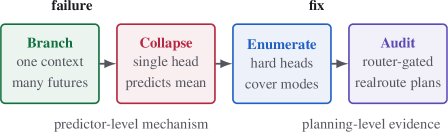
1.0.0.1 Evidence chain.
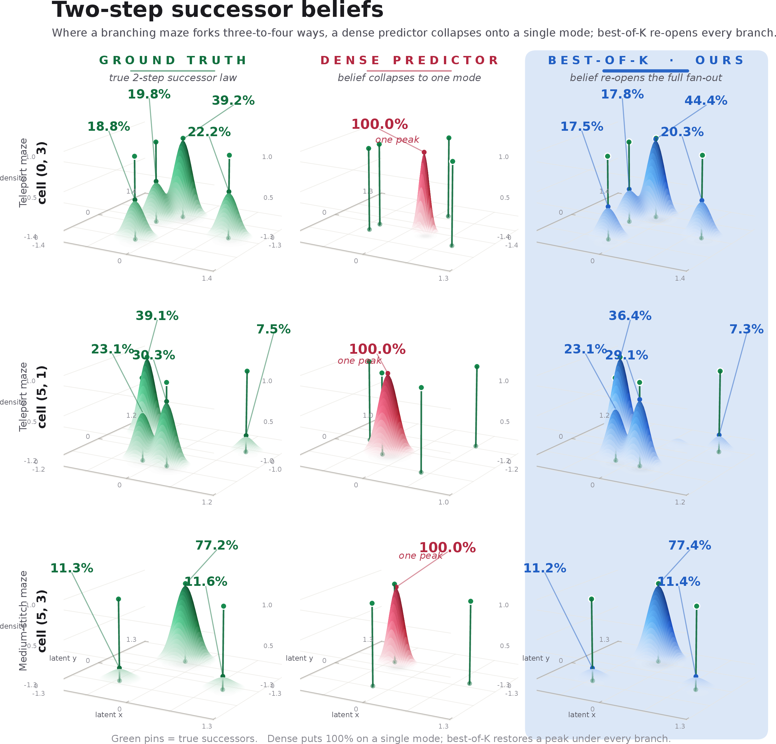
We prove the collapse for deterministic and gated-MoE predictors (Props. 1 and 2), and prove that MoP-JEPA’s hard assignment is a per-context quantizer of the successor distribution (Prop. 3). We then test the mechanism before emphasizing benchmark scores: two-step branchings produce three or four valid successor modes, the dense predictor places one peak, and MoP-JEPA re-opens the fan-out (Fig. 2); antmaze, pixel observations, ETH/UCY, SVHN, and a DINO-WM port check that the phenomenon is not a 2-D maze artifact (Table 1). Finally, we ask whether the recovered modes support planning. Single-output planners reach only \(0.02\)–\(0.09\) success on OGBench stitch and teleport tasks, whereas planning over our enumerated modes recovers (Table 2) and the recovered plans use real transitions (Table 3).
1.0.0.2 Why the audit matters.
Multi-prediction evaluation has a loophole: more samples can cover more outcomes without being context-conditional enough to plan. Our protocol therefore audits everyone, ourselves first, with an input-agnostic codebook control, a shuffled-context test, a router-gated readout, transition-precision guards, and a verified-route criterion in which the model proposes a transition graph blind and ground truth is used only to check whether the route exists. This demotes raw coverage before it adjudicates any baseline.
1.0.0.3 Contributions.
(1) Diagnosis: conditional-mean collapse of deterministic and gated-MoE JEPA predictors under stochastic dynamics. (2) Fix: MoP-JEPA, a hard-assignment multi-predictor head whose loss is the classical multiple-choice / winner-take-all objective [4], [5] but whose role here is world-model mode enumeration. (3) Causal evaluation: a collapse-to-planning measurement chain, with controls, that separates usable context-conditional modes from coverage freeloading.
2 Related Work↩︎
2.0.0.1 JEPA world models.
I-JEPA [6] and V-JEPA [7] established latent-regression prediction; DINO-WM [2] and V-JEPA 2 [3] use the recipe as an action-conditioned world model for planning. Notably, the original JEPA blueprint [1] includes a latent variable whose stated role is to carry exactly the information a multimodal future leaves undetermined — yet every released system above implements the predictor without it, deterministically. We verified this directly on the flagship: loading the released V-JEPA 2-AC checkpoint (a \(305\)M-parameter action-conditioned predictor) with the authors’ own code, the predictor emits a single next-latent per (state, action) — the single-head design our analysis shows collapses under stochastic dynamics. We study what that omission costs and supply the missing component in an enumerable form; we are orthogonal to the encoder and its anti-collapse machinery [8].
2.0.0.2 Probabilistic JEPA.
[9] argue JEPA should be probabilistic and add a variational single-Gaussian predictive distribution; the problem framing is theirs. We benchmark their mechanism (with fixes and a steelmanned implementation; Var-JEPA hereafter, to avoid confusion with Meta’s V-JEPA) and find that a single Gaussian spreads but cannot separate discrete successor modes. Enumerable modes, not samples, are what discrete search consumes.
2.0.0.3 MoE predictors in JEPA.
M3-JEPA [10] implements the predictor as a gated MoE fused by a weighted sum into one output. We prove the fusion collapses identically to the single head (Prop. 2) and confirm this empirically; the fix is the loss (keep \(K\) outputs, assign hard), not the expert count.
2.0.0.4 Multiple-choice and mixture regression.
MCL/WTA [4], [5] and mixture density networks [11] are classical answers to one-to-many regression. Our contribution is the JEPA world-model instantiation, the collapse diagnosis, and the verification protocol; the multimodal-regression literature typically reports oracle coverage without controls, which is the loophole the protocol closes.
2.0.0.5 Offline GCRL (external anchor).
OGBench’s published baselines [12]–[16] solve these tasks with reward-free policy learning. We do not claim to beat this line; we report their published numbers as an external anchor at execution time and note the protocol differences.
3 Setup and Notation↩︎
Offline transitions \(\mathcal{D}=\{(s,a,s')\}\) come from the official OGBench datasets [12]. An encoder \(f_\theta(s)\to z\in\mathbb{R}^d\) is trained with an EMA target copy \(f_\xi\); a predictor \(g\) maps \((z,a)\) to a prediction of \(z'=f_\xi(s')\). Stochastic or stitched data makes the conditional law \(p(z'\mid z,a)\) multimodal: teleport cells map one \((s,a)\) to one of three fixed destinations, and stitched datasets give one state several observed continuations (measured average \(2.1\)–\(2.2\) successor modes per cell). We write \(c=(z,a)\) for the context; \(\mu_1,\dots,\mu_M\) for the \(M\) successor-mode centers with weights \(w_1,\dots,w_M\) and within-mode standard deviation \(\sigma\); and \(\hat{z}' = z'/\lVert z'\rVert\) for normalized targets. The downstream task is goal reaching: plan to the official evaluation goals using only the model (graph search over predicted successors, or model-predictive control in the environment), with success judged without giving the model access to ground truth.
4 Conditional-Mean Collapse↩︎
Proposition 1 (deterministic predictor). Under squared loss the optimal single predictor is \(g^*(c)=\mathbb{E}[z'\mid c]=\sum_m w_m\mu_m\); its error is lower-bounded by the between-mode variance, and for well-separated modes (\(\min_{m\neq m'}\lVert\mu_m-\mu_{m'}\rVert\gg\sigma\)) the optimum lies far from every mode. Under cosine loss with normalized targets and a unit-norm predictor, the exact minimizer is \(u^*=\mathbb{E}[\hat{z}']/\lVert\mathbb{E}[\hat{z}']\rVert\), whose similarity to every mode direction is bounded away from \(1\) whenever the mode directions are mutually separated (Lemma 1, technical appendix).
Proposition 2 (gated MoE). A weighted sum \(\hat{g}(c)=\sum_k \pi_k(c)\,g_k(c)\) outputs a single vector; its objective equals Prop. 1’s with \(v=\hat{g}(c)\). Additional experts and router capacity change which single vector is reachable, not how many are output.
Proposition 3 (best-of-\(K\)). Assume \(M\) well-separated modes with bounded within-mode variance, mode weights bounded away from zero, \(K\geq M\), and predictor heads with sufficient capacity. Then \(L(\{g_k\})=\mathbb{E}\!\left[\min_k\lVert g_k(c)-z'\rVert^2\right]\) is, per context, the \(K\)-means distortion of \(p(\cdot\mid c)\) [17], and every optimum assigns at least one head to each mode, with distortion approaching the within-mode variance. A context-only router trained on the winning index estimates the mode weights. The load-balance and router cross-entropy terms used in training are regularizers outside this statement.
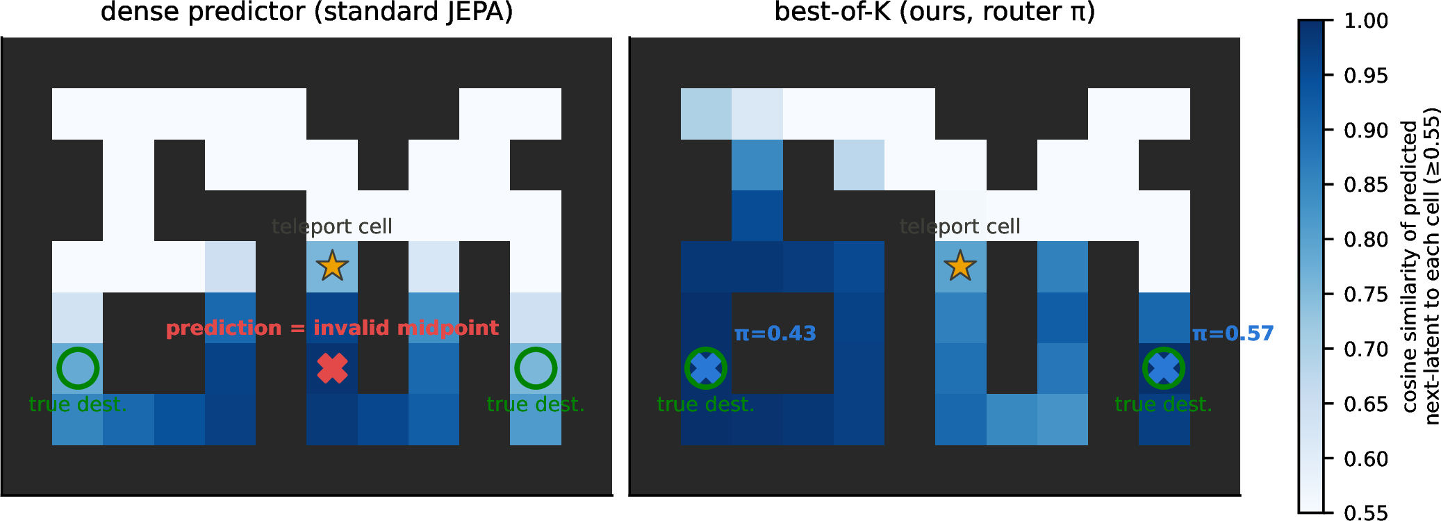
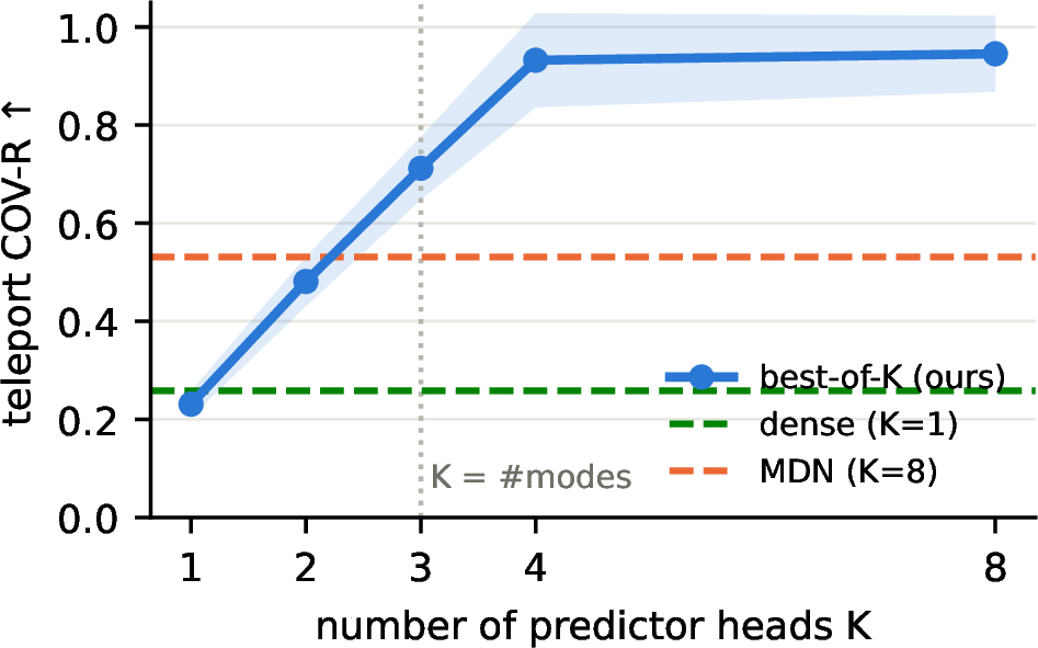
Proofs and the precise separation conditions are in the technical appendix. Figure 2 measures Props. 1 and 3 in the latent space of trained models; Figure 3 shows the same models’ decoded predictions on the maze (a controlled bimodal illustration is in the technical appendix); the \(K\)-sweep of Figure 9 measures the rise-until-\(M\)-then-plateau behavior that Prop. 3 predicts.
5 Method↩︎
5.0.0.1 Variables and standard JEPA objective.
Let \(\mathcal{D}=\{(s_i,a_i,s_i^+)\}_{i=1}^N\) be an offline transition dataset, where \(s_i\in\mathcal{S}\) is the current observation or state, \(a_i\in\mathcal{A}\subseteq\mathbb{R}^{p}\) is the action, and \(s_i^+\) is the observed successor. In domains without actions, \(a_i\) is omitted and the context below is just the current latent. The online encoder is \(f_\theta:\mathcal{S}\to\mathbb{R}^d\) and the target encoder is an exponential-moving-average copy \(f_\xi:\mathcal{S}\to\mathbb{R}^d\). For a minibatch \(\mathcal{B}\), define \[\begin{align} z_i &= \frac{f_\theta(s_i)}{\lVert f_\theta(s_i)\rVert_2},\\ z_i^+ &= \operatorname{sg}\!\left( \frac{f_\xi(s_i^+)}{\lVert f_\xi(s_i^+)\rVert_2}\right),\\ c_i &= [z_i,a_i], \end{align}\] where \(z_i\in\mathbb{R}^d\) is the online context latent, \(z_i^+\in\mathbb{R}^d\) is the stop-gradient target latent, \(c_i\in\mathbb{R}^{d+p}\) is the predictor input, and \(\operatorname{sg}(\cdot)\) stops gradients into the target branch. A standard deterministic JEPA predictor is a function \(g_\phi:\mathbb{R}^{d+p}\to\mathbb{R}^d\) trained by latent regression, \[\begin{align} \mathcal{L}_{\mathrm{dense}}(\theta,\phi;\xi) &= \frac{1}{|\mathcal{B}|}\sum_{i\in\mathcal{B}} \ell\!\left(\bar g_\phi(c_i), z_i^+\right),\\ \bar g_\phi(c)&=\frac{g_\phi(c)}{\lVert g_\phi(c)\rVert_2}, \end{align}\] with cosine distance \(\ell(u,v)=1-u^\top v\) in our implementation. After each optimizer step on \((\theta,\phi)\), the target encoder is updated by \[\xi \leftarrow \tau \xi + (1-\tau)\theta ,\] with EMA momentum \(\tau\) (we use \(\tau=0.996\)). Thus the encoder side is the usual JEPA recipe; the only architectural change below is the predictor.
5.0.0.2 Mixture-of-Predictors parameterization.
MoP-JEPA replaces the single predictor \(g_\phi\) with \(K\) predictor heads \(\{g_{\phi_k}\}_{k=1}^K\), each mapping the same context \(c_i\) to one candidate successor latent. It also learns a context-only router \(r_\psi:\mathbb{R}^{d+p}\to\mathbb{R}^K\). For each example \(i\) and head \(k\), define \[\begin{align} u_{ik} &= \frac{g_{\phi_k}(c_i)}{\lVert g_{\phi_k}(c_i)\rVert_2},\\ \pi_{ik} &= \frac{\exp(r_\psi(c_i)_k)}{\sum_{j=1}^K \exp(r_\psi(c_i)_j)},\\ d_{ik} &= \ell(u_{ik},z_i^+). \end{align}\] Here \(u_{ik}\) is the \(k\)th predicted successor latent, \(\pi_{ik}\) is the router’s deployment-time weight for that head, and \(d_{ik}\) is the distance from that head to the observed target. The router is deliberately restricted to \(c_i\); it never sees \(z_i^+\) and therefore cannot choose a head by peeking at the future.
5.0.0.3 Hard-assignment objective.
For fixed predictions, the latent target assigns itself to the closest head, \[k_i^*=\arg\min_{1\leq k\leq K} d_{ik},\qquad \gamma_{ik}=\mathbf{1}[k=k_i^*],\] where \(k_i^*\) is the winning head and \(\gamma_{ik}\) is its one-hot assignment. The MoP-JEPA loss is \[\begin{align} \mathcal{L}_{\mathrm{MoP}} &= \frac{1}{|\mathcal{B}|}\sum_{i\in\mathcal{B}}\sum_{k=1}^K \gamma_{ik} d_{ik} + \lambda_{\mathrm{route}}\, \frac{1}{|\mathcal{B}|}\sum_{i\in\mathcal{B}} -\log \pi_{i k_i^*}\\ &\quad + \lambda_{\mathrm{bal}}\, \sum_{k=1}^K \bar\gamma_k \log (K\bar\gamma_k), \end{align} \label{eq:mop-loss}\tag{1}\] where \(\bar\gamma_k=|\mathcal{B}|^{-1}\sum_{i\in\mathcal{B}}\gamma_{ik}\) is the minibatch usage of head \(k\), \(\lambda_{\mathrm{route}}\) weights the router cross-entropy, and \(\lambda_{\mathrm{bal}}\) weights the load-balancing penalty \(\operatorname{KL}(\bar\gamma\Vert\mathrm{Unif}(K))\). The first term is the best-of-\(K\) JEPA regression loss. It gives gradient only to the winning head for each target, so with assignments fixed the update for head \(k\) is exactly the ordinary JEPA predictor update restricted to the subset \(\{i:k_i^*=k\}\). The second term trains the router to predict the hard assignment from the context alone; the third prevents unused heads during minibatch optimization. When \(K=1\), Eq. 1 reduces to \(\mathcal{L}_{\mathrm{dense}}\) up to constants.
This is a hard-EM procedure in latent space. The assignment step chooses the nearest current head (\(k_i^*\)), and the update step moves that head toward the assigned target while fitting the router to the same assignments. Under the multimodal conditional law in Prop. 3, this objective is the empirical \(K\)-means distortion of \(p(z^+\mid c)\); hence the heads specialize to distinct successor modes instead of averaging them into one vector.
5.0.0.4 Baselines and protocol.
We compare predictor mechanisms, not codebases. Because none of these predictors has been applied to JEPA world-model planning before, no prior numbers exist for this setting; we therefore reimplement each under one common protocol — identical encoder, offline data, EMA target, and planner — so that the predictor head is the only variable. The arms are: dense (\(K{=}1\), standard JEPA); M3-JEPA [10], its gated mixture-of-experts fused by a weighted sum; Var-JEPA [9], a variational single-Gaussian predictor (steelmanned: cosine-trained mean, residual-calibrated \(\sigma\), \(1/\sqrt d\)-scaled sampling); MDN [11], a soft mixture with load balancing (best of a \(K\times\lambda\) grid); and MoP-JEPA (ours). These are faithful same-protocol reimplementations, not runs of the authors’ released code; the published OGBench GCRL numbers we quote later are used only as an external anchor, never as a same-protocol comparison.
5.0.0.5 Prediction interface.
At test time the model receives only \((s,a)\). It computes \(z=f_\theta(s)/\lVert f_\theta(s)\rVert_2\), \(c=[z,a]\), and emits the set \[\begin{align} \mathcal{P}(s,a)&=\{(u_k,\pi_k)\}_{k=1}^K,\\ u_k&=\frac{g_{\phi_k}(c)}{\lVert g_{\phi_k}(c)\rVert_2},\\ \pi_k&=\operatorname{softmax}(r_\psi(c))_k . \end{align}\] The output is therefore an enumerable successor set in one forward pass, not samples from a post-hoc decoder and not a weighted average. A downstream planner or evaluator can consume all heads, or only router- active heads above a fixed threshold, without access to the realized successor.
6 Verification Protocol↩︎
Multi-prediction can look good by covering outcomes for free, so every positive result is audited. We use planAll for model-internal graph searchability and official-goal success for held-out goals, but the load-bearing metric is realroute: the model first proposes a transition graph blind, and ground truth is used only afterward to check whether a route made entirely of real transitions exists inside that proposal. Transition precision guards against graph inflation by non-existent edges, and execution success runs the planner closed-loop in the environment. Three controls separate usable mode enumeration from freeloading: an input-agnostic codebook, an off-context shuffle test, and router gating, where only heads with context-predicted mass \(\pi_k>0.5/K\) count.
7 Experiments↩︎
7.0.0.1 Setup.
Official OGBench offline datasets: pointmaze-medium-stitch, pointmaze-large-stitch, pointmaze-teleport-navigate, and antmaze-teleport (29-D). Leak-free evaluation: coordinate features (no cell-identity memorization) and \(20\%\) of unique transitions held out of training. Five seeds for planning, three for coverage and execution; tables give mean\(\pm\)std over seeds and figures show per-seed points. No metric gives the model access to ground truth at decision time.
7.1 Evidence Chain and Generality↩︎
The central question is not whether one predictor variant wins one maze benchmark, but whether the same mechanism repeats across stochastic predictors, branching degrees, and domains. Table 1 summarizes the evidence chain we test before reporting planner scores; Fig. 4 plots the three main diagnostics.
| Link in the chain | Evidence in the paper |
|---|---|
| Collapse | Dense/gated-MoE emit one latent mean; the decoded maze state is an invalid midpoint (Figs. [fig:bimodal], [fig:maze]). |
| Specialization | MoP-JEPA re-opens three/four-way fan-outs; independently trained heads collapse to the same mean. |
| Branching complexity | Coverage rises until \(K\) matches the mode count; two-step cells expose the rare-mode ceiling. |
| Generality | ETH/UCY, SVHN, antmaze, pixel observations, and DINO-WM show the same mechanism beyond 2-D point mazes. |
| Planning consequence | Realroute verifies that enumerated modes form a searchable graph of real transitions. |
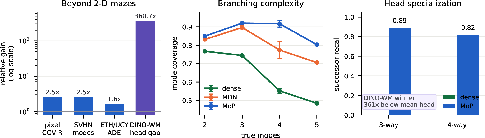
The same collapse and fix appear beyond low-dimensional mazes. On a genuine JEPA latent forecaster (ETH/UCY pedestrians [18], leave-one-scene-out) the mixture beats the codebook control on every scene and seed (\(0.053\) vs.\(0.070\) vs.dense \(0.118\), shuffle \(2.0\times\)), and on raw multimodal regression it improves pedestrian forecasting (\(+37.7\%\)) and image inpainting (\(+24.1\%\)), both fully context-conditional under the controls. Conversely, standard masked-SSL pretext is near-deterministic given context: there is no collapse to fix and multiple predictors tie the single one. This scopes the contribution precisely: JEPA as a forecaster or world model of genuinely multimodal futures.
The mechanism also transfers to a second codebase and to image observations. Porting the head into DINO-WM’s official world model [2] is a one-line predictor override (predictor=mixture) with no other pipeline change; it trains as a drop-in, and its heads specialize rather than duplicate — on held-out pixel point-maze the winning head’s
next-latent error is two orders of magnitude below the head average, with \(\approx\!2\) heads active per state, matching the maze’s local branching factor. On masked-digit SVHN (real images, bottom-half
inpainting), the deterministic head realizes only \(0.31\) of the conditional digit-modes while the mixture heads realize \(0.78\) (\(2.5\times\), 3 seeds);
density and ensemble baselines reach \(0.85\)–\(0.89\) but expose no enumerable, router-gated successor set to plan through.
Finally, the collapse and its fix persist as the number of futures grows. Aggregated over all three- and four-way two-step maze cells (\(3\) seeds, technical appendix), MoP-JEPA recovers \(82\)–\(88\%\) of the successors while the dense predictor recovers none: its single mean prediction lands between the modes, on no valid state. The hard-assigned heads retain even low-probability (\(<\!10\%\)) successors; the residual gap is a rare-mode ceiling at four-way branching (a single tail mode missed in some cells), consistent with the winner-take-all limit we report in the limitations.
7.2 Planning on the Predicted Graph↩︎
| planAll \(\uparrow\) | med-stitch | teleport | large-stitch |
|---|---|---|---|
| dense (JEPA) | .084\(\pm\).03 | .037\(\pm\).01 | .016\(\pm\).01 |
| M3-JEPA | .075\(\pm\).02 | .036\(\pm\).01 | .031\(\pm\).01 |
| Var-JEPA | .085\(\pm\).01 | .035\(\pm\).01 | .033\(\pm\).00 |
| MDN | .566\(\pm\).20 | .512\(\pm\).12 | .717\(^{\dagger}\)\(\pm\).12 |
| MoP-JEPA (ours) | .851\(\pm\).08 | .748\(\pm\).09 | .386\(\pm\).45 |
| codebook (control) | .267\(\pm\).02 | .167\(\pm\).02 | .149\(\pm\).04 |
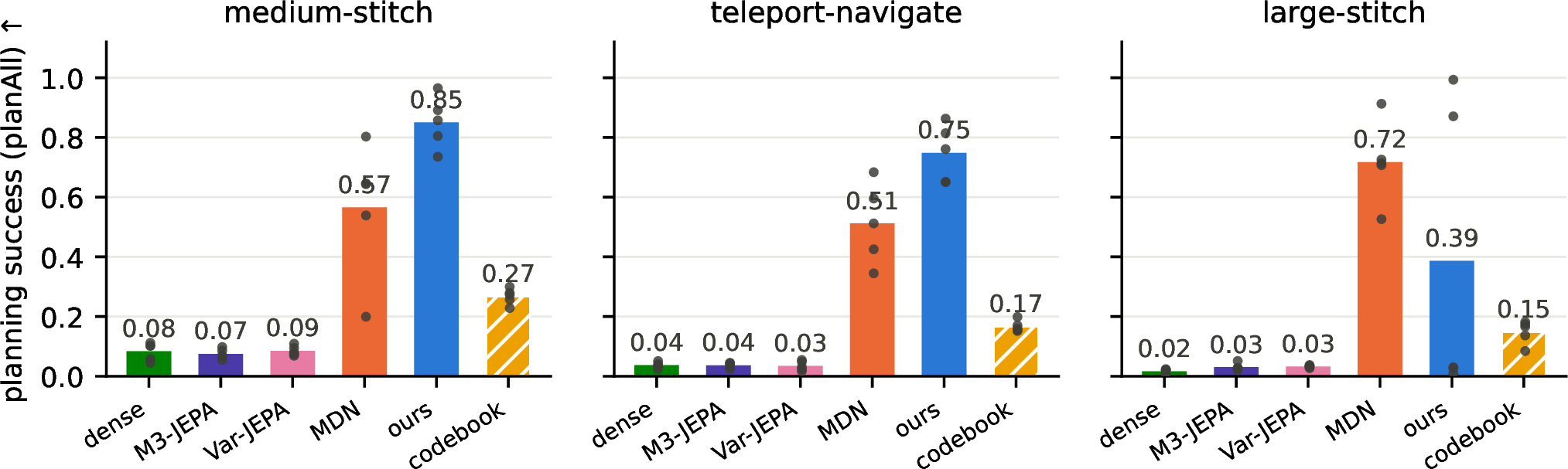
Table 2: deterministic, gated-MoE, and Var-JEPA predictors reach \(0.02\)–\(0.09\), consistent with Props. 1–2; ours reaches up to \(0.85\).
7.3 Adjudication: Verified Routes↩︎
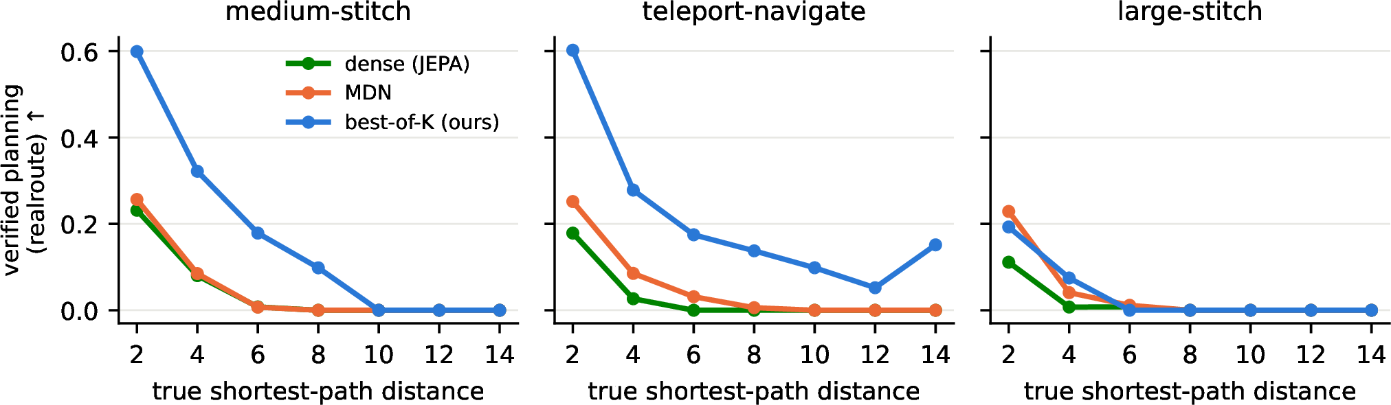
MDN’s raw numbers depend on predicted edges that do not exist: its transition precision is \(0.14\)–\(0.21\) (ours \(0.42\)–\(0.56\)), and graph search will happily route through hallucinated walls. Under realroute, all three mazes favor ours (Table 3, Fig. 6). The paired advantage over MDN is statistically significant on medium-stitch (bootstrap \(95\%\) CI of the per-seed difference \([0.06, 0.18]\)) and teleport (\([0.07, 0.24]\)); on large-stitch the mean favors ours but the CI includes zero at five seeds, reflecting the seed-bimodality we report below. Under fully matched capacity and training (\(K{=}16\), \(60\)k steps, \(5\) seeds, both arms’ best load-balance settings) the large-stitch verdict is unambiguous: ours reaches realroute \(0.208\) vs.MDN’s \(0.095\) (\(2.2\times\)), with MDN’s found rate high (\(0.88\)) but precision low (\(0.21\)) — it routes through non-existent edges — against our \(0.42\) precision. More capacity buys the MDN more hallucinated edges, not more real routes.
| realroute \(\uparrow\) | dense | MDN | MoP-JEPA |
|---|---|---|---|
| medium-stitch | .083\(\pm\).03 | .134\(\pm\).03 | .247\(\pm\).08 |
| teleport-navigate | .035\(\pm\).01 | .039\(\pm\).01 | .192\(\pm\).09 |
| large-stitch | .016\(\pm\).01 | .057\(\pm\).03 | .139\(\pm\).15 |

7.3.0.1 Long horizons.
Fig. 7: at distance \(6\) on medium-stitch ours retains \(0.18\) verified success versus MDN’s \(0.01\); on teleport, where long routes cross the stochastic branching repeatedly, ours holds \(0.05\)–\(0.15\) out to distance \(14\) while both baselines reach zero by distance \(6\)–\(8\). Mode errors compound multiplicatively with rollout depth, which is why a mode-faithful one-step predictor is the load-bearing requirement for long-horizon planning.
7.3.0.2 Is the MDN under-tuned?
A fairness grid over components \(K\in\{8,16\}\) and load-balance weight \(\lambda\in\{0,0.01,0.1\}\) (learned \(\sigma\) throughout, 3 seeds each) leaves the ordering unchanged on every task: the strongest variant reaches realroute \(0.125\) on medium (ours \(0.247\)) and \(0.114\) on teleport (ours \(0.192\)). On large-stitch, strong load-balancing genuinely helps MDN (best variant \(0.191\)); under fully matched capacity and training it remains behind ours.
7.4 Verified Planning Across the JEPA Predictor Family↩︎
| verified planning (realroute) \(\uparrow\) | execution \(\uparrow\) | ||||
|---|---|---|---|---|---|
| 2-4(lr)5-6 JEPA predictor (same encoder, data, planner) | med-stitch | teleport | large-stitch | med | large |
| dense (standard JEPA) | .083 | .035 | .016 | .27 | .13 |
| M3-JEPA | .075 | .036 | .031 | — | — |
| Var-JEPA (variational) | .034 | .001 | .033 | — | — |
| MDN (best of a \(K\times\lambda\) grid) | .134 | .039 | .095 | .87 | .27 |
| MoP-JEPA (ours) | .247 | .192 | .208 | .67 | .33 |
The family comparison is same-protocol by construction: every arm shares the encoder, the offline data, and the planner, and differs only in the predictor head, so Table 4 isolates the effect of the predictor’s output distribution. Our executor is verified sound (\(15/15\) on true paths; on a truth graph corrupted with \(10\%\) false edges, replanning lifts success \(0.40\to1.00\)), and a uniform-edge-cost ablation leaves all execution rankings unchanged. The published-baseline numbers are quoted only as external context, not a same-protocol comparison; the load-bearing result is that a one-line predictor change turns a world model that cannot plan into one that plans verifiably.
7.5 Coverage of Stochastic Dynamics↩︎
| pointmaze-teleport | raw | \(\pi\)-gated | COV-P | shuffle |
|---|---|---|---|---|
| dense | .244\(\pm\).03 | .244\(\pm\).03 | .733 | 2.4\(\times\) |
| M3-JEPA | .242\(\pm\).04 | .242\(\pm\).04 | .727 | 1.4\(\times\) |
| Var-JEPA | .001\(\pm\).00 | .001\(\pm\).00 | .000 | — |
| MDN | .596\(\pm\).02 | .292\(\pm\).01 | .864 | 1.8\(\times\) |
| MoP-JEPA | .997\(\pm\).00 | .632\(\pm\).22 | .924 | 2.4\(\times\) |
| codebook | 1.00\(\pm\).00 | 1.00\(^{\ddagger}\) | .417 | 1.0\(\times\) |
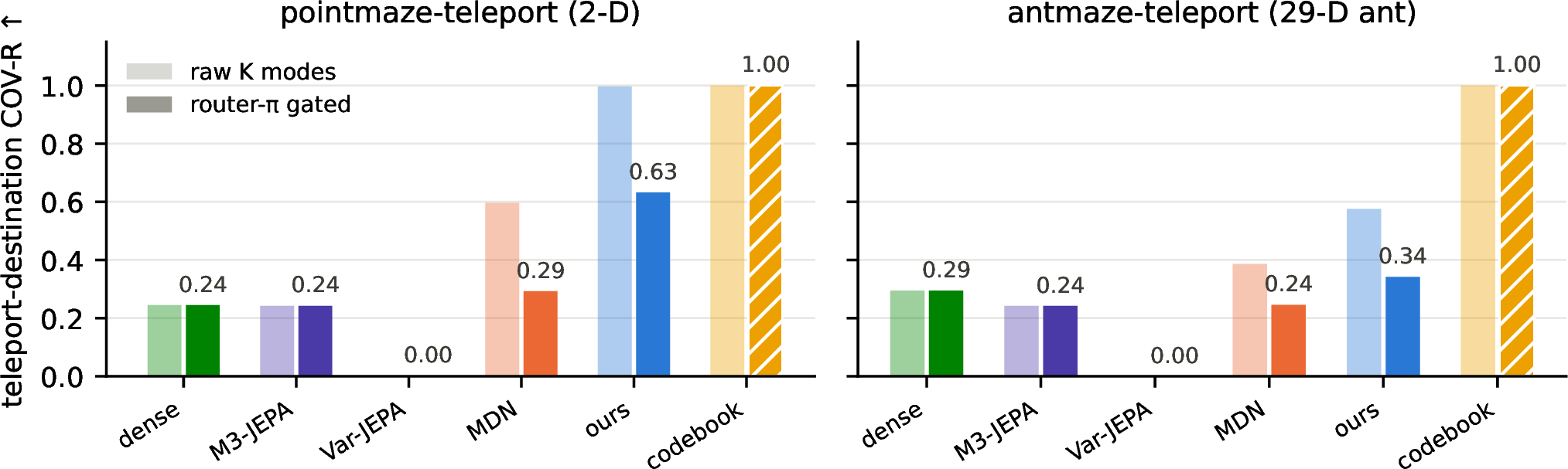
Destinations are fixed global states, so the input-agnostic codebook maxes raw COV-R at \(1.0\); our own protocol flags naive coverage as freeloading. The verdict is threshold-insensitive: sweeping the gate over \(t\in[1/64,1/4]\), our gated coverage degrades gracefully (\(0.74\to0.40\)) while precision (\(\approx0.92\)) and shuffle leakage (\(\approx0.26\)) stay flat, and every baseline is invariant or pinned below. On antmaze-teleport (29-D ant, destinations as manifolds of 32 real samples) the ranking persists with honest attenuation: ours \(0.576\) raw, about \(2\times\) dense (\(0.294\)) and \(1.5\times\) MDN (\(0.386\)); gated \(0.342\) at \(0.86\) precision; Var-JEPA \(0\). On pixel observations (visual-antmaze-teleport, \(64{\times}64{\times}3\); CNN JEPA trained from scratch, teleport transitions oversampled identically for every arm), the ranking again persists: ours \(0.613\) raw COV-R vs. \(0.24\)–\(0.27\) for every baseline (\(2.4\times\)), with partial mode recovery (gated \(\approx 1\) of 3 modes at \(0.97\) precision). High-dimensional and pixel-level JEPA world models capture the branching direction but not yet full mode-fidelity; closing that gap is open.
7.6 Summary and Ablations↩︎
| modes | COV-R | prec. | real- | exec | |
| enum.? | (gated) | route | (hard) | ||
| dense | no | .24 | high | 0/3 | .13 |
| M3-JEPA | no | .24 | high | 0/3 | — |
| Var-JEPA | samples | .00 | — | 0/3 | — |
| MDN | soft | .29 | .14–.21 | 0/3 | .27 |
| MoP-JEPA | yes | .63 | .42–.56 | 3/3 | .33 |
| codebook | static | n/a | — | 0/3 | — |
7.6.0.1 \(K\)-sweep (real data).
Teleport COV-R rises from \(0.231\) at \(K{=}1\) (matching dense \(0.258\)) to \(0.712\) at \(K{=}3\) (the number of modes) and plateaus at \(0.945\) by \(K{=}8\) (MDN at \(K{=}8\): \(0.531\)).
7.6.0.2 Design ablations.
An explicit head-separation loss is redundant (WTA already separates, and it can hurt recall). Slow soft-to-hard annealing over \(80\%\) of training drags every head toward the mean; a fast warmup accelerates small-model convergence dramatically while plain hard EM is already sufficient at full scale. An ensemble of \(K\) independently trained heads (no assignment) collapses entirely: realroute \(0.03\)–\(0.10\), at dense level, with zero spread across heads — each head converges to the same conditional mean, Prop. 1 applied \(K\) times. Independence is not diversity; hard assignment is the load-bearing design choice.
7.7 The Protocol Fires Where It Should↩︎
It audits the strongest baseline: MDN’s raw planning scores are traced to non-existent predicted edges (§Adjudication). It audits us: raw coverage is demoted as freeloadable (Table 5). It detects metric artifacts: on antmaze, full-observation destination centroids score every arm and every control at exactly zero, the fingerprint of an off-manifold reference point (ant joints are arbitrary at a fixed-\(xy\) destination), which we caught and replaced with real-sample manifolds. It rejects illusory multimodality: on road-constrained taxi forecasting an apparent \(+36\%\) gain is \(84\%\) reproducible by the codebook (shuffle \(1.23\times\)) and is rejected; on persistence-dominated next-frame video no gain is claimed. The verdict tracks whether futures genuinely branch, which is what makes the positive results trustworthy.
8 Discussion and Limitations↩︎
8.0.0.1 Why this matters for scaling JEPA world models.
Video- and robot-scale world models [2], [3] are trained on data where stochasticity is the rule. Our results indicate that the deterministic predictor’s failure there is not graceful: the error concentrates on exactly the branchings a planner must resolve, and it silently produces states that do not exist. The broader lesson is that a stochastic world model should expose a set-valued transition interface, not only a latent expectation. MoP-JEPA is one minimal implementation of that interface: a head-level change, orthogonal to encoder architecture and scale, that yields enumerable branch outcomes with calibrated router weights. The verification protocol is architecture-agnostic: any world model that emits multiple futures (mixture, variational, diffusion, or generative) can be audited with the same suite, and we would encourage its adoption wherever multi-sample prediction numbers are reported.
8.0.0.2 Limitations.
The claim concerns the transition distribution and what it enables; single-shot selection of an aleatoric branch is impossible for any model and is not claimed. WTA optimization on the hardest maze is seed-bimodal, and at four-way two-step branching a rare (\(<\!10\%\)) successor can fall below head activation and be missed (full four-mode recovery in \(37\%\) of such cells); annealing does not fix it at scale, an explicit head-repulsion regularizer hurts, and head-wise learning rates or replay biased toward rare modes remain untested. Mazes are low-dimensional state spaces; the 29-D ant extends the mechanism with attenuation, and the DINO-WM port confirms the head-level fix on pixel observations, though scaling the verification protocol to video- and robot-scale world models remains future work. Comparisons within the predictor family are same-protocol reimplementations (no prior numbers exist for these predictors in this setting); the published-baseline anchor is quoted, not rerun, and is not a same-protocol comparison.
9 Conclusion↩︎
A deterministic JEPA world model cannot represent a stochastic branching: it predicts a latent expectation where planning needs enumerable futures. We prove this conditional-mean collapse, show it across branch counts and beyond 2-D mazes, and measure the planning failure it causes. Hard-assigned predictors recover one successor mode each, turning the predictor output from a single invalid average into a searchable transition set; verified planning succeeds when that set contains real routes. The method is deliberately minimal, but the point is broader: stochastic JEPA world models need mode enumeration, and claims about multimodal prediction should be audited for context-conditional, real-transition structure rather than raw oracle coverage.