TARE: Tail Aware Evaluation of HPC Job Runtime Prediction
January 01, 1970
Abstract
Runtime estimates affect reservation quality, backfilling opportunities, and queue delay in HPC schedulers. Under heavy tailed workloads, however, averaging over jobs can misrepresent scheduling impact because a small fraction of jobs dominates resource
usage. This paper presents an empirical evaluation methodology for HPC job runtime prediction that focuses on the tail, combining GeoAccuracy weighted by resource usage with decile and split analyses. Using production traces from NREL Eagle and ALCF
Mira/Intrepid, we compare XGBoost and Last2 against the user provided walltime estimate at submission (UserReq). Across all three datasets, evaluation focused on the tail changes the offline conclusion: MeanAccuracy
keeps the methods relatively close, whereas GeoAccuracy reveals clearer separation and makes UserReq’s strength in the upper tail visible. In the top decile, UserReq achieves the highest GeoAccuracy and lowest underestimation rate
on all three datasets, and this pattern remains stable across rolling splits. We then translate this signal into a simple hybrid scheduling policy that keeps XGBoost for most jobs and routes the top decile by proxy_cost at
submission to UserReq. Online replay on four production queues reduces mean wait time by up to 8% and increases backfilled jobs by 50%–115%. These results show that offline evaluation focused on the tail better characterizes prediction quality
relevant to scheduling and informs scheduling policy design.
1 Introduction↩︎
In batch scheduled HPC systems, users submit jobs with requested resources such as node counts and walltime limits, and those jobs wait in queue until the scheduler selects them for execution. Under FCFS with EASY backfilling,
the scheduler uses a runtime estimate to reserve resources for the job at the head of the queue and to determine whether later jobs can start early without delaying that reservation [1], [2]. Runtime estimation therefore affects
reservation quality, backfilling opportunities, and queue performance directly. Overestimation can leave schedulable gaps unused, while underestimation can make planned reservations less reliable. For this reason, HPC job runtime prediction has long been
studied as a scheduling problem rather than only as a forecasting problem [3], [4].
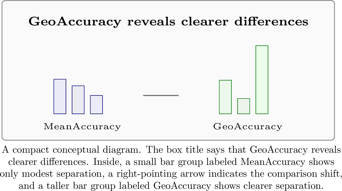
Because runtime estimates directly affect scheduling decisions, evaluating their quality is itself a scheduling problem. Most runtime prediction studies focus on predictor design and report aggregate accuracy at the job level. But the practical significance of a prediction error depends on which jobs incur it. If a workload has heavy tails, a small fraction of jobs can dominate resource usage. That property is central here: averaging over jobs can obscure the errors with the greatest scheduling consequences. We therefore ask whether weighting accuracy by resource usage reveals predictor differences that job averaged evaluation keeps much closer together. Figure 1 previews this comparison. We compare the weighted geometric metric GeoAccuracy, \(A_{\mathrm{geo}}\), with its arithmetic mean counterpart over jobs, MeanAccuracy, \(A_{\mathrm{mean}}\). We study two runtime predictors and compare them with the user provided walltime estimate at job submission:
XGBoost, a machine learning predictor;Last2, a heuristic baseline; andUserReq, the user provided walltime estimate at job submission.
We compare these three methods on three production workload datasets: Eagle from NREL and Mira/Intrepid from the Argonne Leadership Computing Facility (ALCF) [5], [6]. All three come from large production HPC
systems at national laboratories. Shared preprocessing yields aligned prediction sources. We then apply a consistent offline evaluation across all three datasets and use its findings to design an online replay study on Mira and
Intrepid.
Before comparing metrics, we verify the workload property that motivates the study in these three traces. A heavy tailed resource usage pattern is not a new discovery of this paper. Prior HPC workload characterization studies have repeatedly reported
strong skew and heterogeneity in job size, resource usage, and workload structure on large HPC systems [6]–[8]. Our purpose is to show that the same concentration appears in Eagle, Mira, and
Intrepid, and to quantify its magnitude. Figure 2 shows that the highest decile alone contributes about 81%–87% of total resource usage across the three datasets. Because HPC resources are scarce and
scheduler impact is dominated by large, long running jobs, that concentration makes upper-tail behavior especially important. The CDF view in Figure 2 (b) shows the same concentration from a continuous distribution
perspective: Eagle sits farther to the upper left because its jobs consume much smaller node hours, whereas Mira and Intrepid lie farther to the lower right and remain close because the two ALCF traces have similarly
large job scales.


Figure 2: Evidence of a heavy tail. The highest 10% alone contributes about 81%–87% of total resource usage across the three datasets.. a — Equal sized decile., b — Empirical CDF of node hours.
Under a workload with heavy tails, averages over jobs give every job the same influence, whereas averages weighted by resource usage give more influence to the jobs that consume most node time. As a result, the same method comparison can support
different overall conclusions. In our data, \(A_{\mathrm{mean}}\) keeps the three methods much closer together, whereas \(A_{\mathrm{geo}}\) reveals much clearer differences and makes
UserReq’s strength in the upper tail visible on all three datasets. This result is notable because UserReq is the user provided walltime estimate at job submission rather than a learned predictor, but the explanation is that \(A_{\mathrm{geo}}\) emphasizes the upper tail of resource usage, where UserReq performs better. This difference also remains stable across most rolling split days, so it is not an artifact of a small sample.
The paper follows a three part experimental workflow: shared data preparation, offline evaluation, and online simulation. The offline evaluation weights errors by resource usage and analyzes the upper tail explicitly; the online simulation then tests whether this offline upper-tail signal translates into scheduling outcomes. This emphasis comes from the workload weights and upper-tail analysis, not from any special outlier sensitivity of the geometric mean alone.
The contribution is empirical and evaluative rather than algorithmic. We do not propose a new predictor. Instead, this study makes three contributions:
We present an empirical evaluation methodology for HPC job runtime prediction that focuses on the tail. It combines GeoAccuracy weighted by resource usage with decile and split level analyses, so offline evaluation reflects the jobs that dominate scheduling impact rather than averages over jobs alone.
Using three production workload datasets, we show that evaluation focused on the tail changes the overall comparison of runtime predictors. MeanAccuracy keeps the methods much closer together, whereas GeoAccuracy reveals clearer separation and makes
UserReq’s strength in the resource dominant upper tail visible. In the top decile,UserReqachieves the highest GeoAccuracy and the lowest underestimation rate on all three datasets, and this advantage remains stable across rolling split days.We translate this offline signal into a simple hybrid scheduling policy and show in online replay that it improves scheduling performance. The policy keeps
XGBoostfor most jobs and routes the top decile of jobs byproxy_cost, computed from requested nodes and walltime at submission, toUserReq. Across the short and long production queues on two HPC systems, this policy reduces mean wait time by up to 8% and increases backfilled jobs by 50%–115%.
The rest of the paper is organized as follows. Section 2 presents the methodology, including the offline evaluation metrics and the offline analysis procedure. Section 3 describes the experimental setup, including data preparation, datasets, predictors, and the rolling split offline evaluation procedure. Section 4 presents the offline results, including the overall metric comparison, analysis of the upper tail, and robustness at the split level. Section 5 presents the online simulation, including its design and results. Section 6 reviews related work, and Section 7 concludes the paper.
2 Methodology↩︎

2.1 Offline Evaluation Metrics↩︎
In the batch queue setting, a submitted job carries requested resources and a user walltime estimate, then later yields an observed actual runtime after execution. For job \(i\), let \(y_i\) denote the actual runtime, \(\hat{y}_i\) the predicted runtime, and \(c_i = \texttt{nodes\_req} \times \texttt{runtime\_act}\) denote the resource usage used as the offline weight.
We use multiplicative error rather than additive error because HPC job runtimes span a wide range of scales. An additive error measured in seconds is therefore not directly comparable across jobs: the same absolute miss can be minor for a long job but severe for a short job. Taking a log ratio turns multiplicative misses into additive quantities, so ratio errors can be averaged cleanly across jobs. It also treats paired ratio errors symmetrically, so predicting \(2y_i\) and \(y_i/2\) yields the same penalty. This keeps relative prediction quality separate from the weights by resource usage introduced later in \(A_{\mathrm{geo}}\). The basic log ratio error is \[e_i = \left| \log \frac{\hat{y}_i}{y_i} \right|.\] Because the shared preprocessing keeps only jobs with observed runtime above 30 s and the evaluation retains only valid positive predictions, every analyzed row satisfies \(y_i > 0\) and \(\hat{y}_i > 0\). We therefore do not need a separate branch for zero runtime in the metric definition.
The accuracy score for each job is \[a_i = \exp(-e_i) = \min\left(\frac{\hat{y}_i}{y_i}, \frac{y_i}{\hat{y}_i}\right).\] This yields the familiar arithmetic mean metric over jobs \[A_{\mathrm{mean}} = \frac{1}{N} \sum_{i=1}^{N} a_i.\] Throughout the paper, we refer to \(A_{\mathrm{mean}}\) as MeanAccuracy.
To emphasize jobs with high resource usage, we also define the log error weighted by resource usage \[L_{\mathrm{usage}} = \frac{\sum_i c_i e_i}{\sum_i c_i}.\] The corresponding weighted geometric metric is \[A_{\mathrm{geo}} = \exp(-L_{\mathrm{usage}}) = \prod_i a_i^{\,c_i / \sum_j c_j},\] which is the weighted geometric mean of the job level accuracy scores \(a_i\). Throughout the paper, we refer to \(A_{\mathrm{geo}}\) as GeoAccuracy.
The log form is what makes the geometric mean natural here. Averaging \(e_i\) summarizes a typical multiplicative miss on an additive scale, and exponentiating back returns the result to the same \((0,1]\) accuracy scale as \(A_{\mathrm{mean}}\). GeoAccuracy is therefore not an arbitrary alternative summary: it is the consistent aggregate of multiplicative error under weights by resource usage.
The emphasis on the workload tail comes from the weights \(c_i\), not from the use of a geometric mean by itself. GeoAccuracy emphasizes the tail because it weights jobs by resource usage and places most mass on the upper tail of that distribution. It does not make the metric inherently more sensitive to extreme error outliers.
This distinction matters because MeanAccuracy and GeoAccuracy answer different questions. MeanAccuracy is an average over jobs. GeoAccuracy is weighted by resource usage and therefore emphasizes the part of the workload whose resource usage most strongly affects scheduling outcomes.
To explain the overall metric difference, we also evaluate predictors on equally sized deciles of offline resource usage. Within each dataset, we sort jobs by \(c_i\) and divide them into ten equally sized groups; the tenth group is the top decile. This decile view complements the overall metrics: it explains why GeoAccuracy can reveal clearer differences than MeanAccuracy and localizes the upper tail discussed later in the paper. When the online section later refers to a p90 or top decile routing rule, it uses the same percentile language but applies it to the proxy \(\texttt{proxy\_cost}\) at submission within each queue-year partition, rather than to the offline resource usage variable \(c_i\).
We also report the underestimation rate \[\mathrm{UnderRate} = \frac{1}{N} \sum_i \mathbf{1}[\hat{y}_i < y_i].\]
UnderRate is useful because it exposes a different failure mode from the accuracy metrics. A predictor can achieve competitive MeanAccuracy or GeoAccuracy while still underestimating actual runtime too often. We therefore treat MeanAccuracy, GeoAccuracy, and UnderRate as complementary rather than redundant summaries.
Accordingly, the offline evaluation proceeds in three steps. It first compares the overall metrics on the valid rows of each model, then analyzes equally sized deciles of resource usage within each dataset to isolate the highest decile, and finally checks whether the corresponding metric gaps at the split level remain stable across rolling split days. These offline results then motivate the online simulation reported later.
3 Experimental Setup↩︎
Figure 3 summarizes the experimental workflow. This section covers its first two parts: shared data preparation and rolling split offline evaluation on all three datasets. Section 5 then uses the same traces in online replay, which preserves the observed chronology of job arrivals and changes only the planned runtimes seen by the scheduler.
3.1 Data Preparation and Date Ranges↩︎
We study three production traces from systems at national laboratories: Eagle at NREL and Mira/Intrepid at ALCF [5], [6]. Shared data preparation organizes the raw traces around common submit, start, end, and resource request fields;
removes invalid or incomplete rows while retaining jobs with valid terminal states; constructs the inputs available at submission that are used by the predictors, including each user’s recent job history needed by Last2; applies the common
runtime filter runtime > 30 s; aligns the three prediction sources on consistent jobs; and defines rolling split days after a 100 day warm up window.
Their raw submit time spans are 2018-11 to 2023-02 for Eagle, 2014-10 to 2018-12 for Mira, and 2009-12 to 2013-12 for Intrepid. Following the prior Eagle runtime prediction workflow [5], the offline evaluation uses daily rolling splits with a 100 day training window, so evaluated split days begin only after the first 100 days of
history. The resulting ranges of split days are 2019-02 to 2023-02 for Eagle, 2015-02 to 2018-12 for Mira, and 2010-03 to 2013-12 for Intrepid. After filtering and alignment of prediction sources, the offline
evaluation contains 7,267,468 jobs and 1,435 rolling splits for Eagle, 242,753 jobs and 1,425 splits for Mira, and 271,713 jobs and 1,379 splits for Intrepid.
3.2 Runtime Predictors and User Estimate↩︎
The two runtime predictors and the user provided walltime estimate at job submission play distinct roles. XGBoost is a gradient boosted tree predictor and a strong representative choice for tabular runtime prediction tasks [5], [9], [10]. Last2 is a heuristic baseline that predicts a job as the mean runtime of the same user’s two most recent jobs in the training window, with fallback to the global
recent job mean when that user has no history [4]. UserReq uses the submitted walltime request
wallclock_req directly.
3.3 Offline Evaluation Procedure↩︎
Each rolling split trains on jobs whose end_time lies in the previous 100 days and tests on jobs whose submit_time lies in the next 1 day. For split day \(t\), the training window is \([t-100\text{ days}, t)\) in end_time and the test window is \([t, t+1\text{ day}]\) in submit_time. Advancing \(t\) by one day creates
a time ordered sequence of metrics rather than a single random holdout. Decile boundaries are computed once per dataset by sorting jobs by resource usage and splitting them into ten equally sized groups; the same boundaries are then applied to all
models.
At the split level, the analysis unit is each rolling split day rather than individual jobs, and comparisons use the split days where both predictors have valid offline metrics. For each metric, we summarize the fraction of common split days where one predictor outperforms the other: higher values win for metrics such as \(A_{\mathrm{mean}}\) and \(A_{\mathrm{geo}}\), while lower values win for metrics such as UnderRate.
4 Offline Results↩︎
4.1 Evaluation Focused on the Tail Changes the Offline Conclusion↩︎
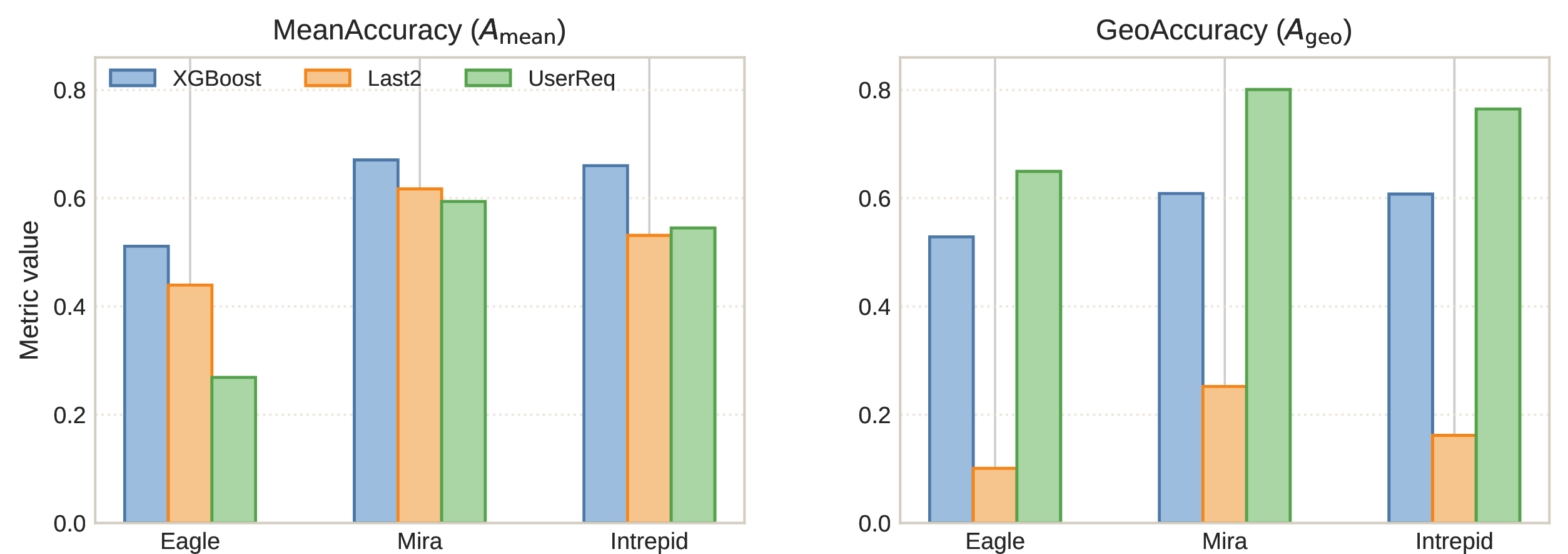
With the heavy tail workload property established in Section 1, Table 1 and Figure 4 report the main overall metrics. The key result is that evaluation focused on the tail
changes the offline conclusion. Under \(A_{\mathrm{mean}}\), the methods remain much closer together, whereas \(A_{\mathrm{geo}}\) separates them much more clearly. The gap between the
maximum and minimum across the three models increases from 0.242 to 0.549 in Eagle, from 0.077 to 0.549 in Mira, and from 0.129 to 0.603 in Intrepid when moving from \(A_{\mathrm{mean}}\) to \(A_{\mathrm{geo}}\).
This larger separation makes the effect of the workload tail visible at the overall metric level. Under \(A_{\mathrm{mean}}\), the three methods stay close together, especially in Mira and
Intrepid. Under \(A_{\mathrm{geo}}\), Last2 drops sharply and UserReq pulls clearly away from the others. The ranking change is therefore a consequence of stronger separation in the
tail; the more fundamental point is that evaluation weighted by resource usage reveals much larger performance differences among the methods from a scheduling perspective.
| Dataset | Model | \(A_{\mathrm{mean}}\) | \(A_{\mathrm{geo}}\) | \(\mathrm{UnderRate}\) |
|---|---|---|---|---|
| Eagle | XGBoost | 0.511 | 0.529 | 39.9% |
| Last2 | 0.440 | 0.101 | 52.5% | |
| UserReq | 0.269 | 0.650 | 11.0% | |
| Mira | XGBoost | 0.671 | 0.609 | 54.0% |
| Last2 | 0.617 | 0.252 | 50.3% | |
| UserReq | 0.594 | 0.801 | 17.1% | |
| Intrepid | XGBoost | 0.660 | 0.608 | 48.7% |
| Last2 | 0.531 | 0.162 | 55.8% | |
| UserReq | 0.545 | 0.765 | 11.5% |
2.5pt
4.2 Analysis of the Upper Tail Explains Why the Conclusion Changes↩︎
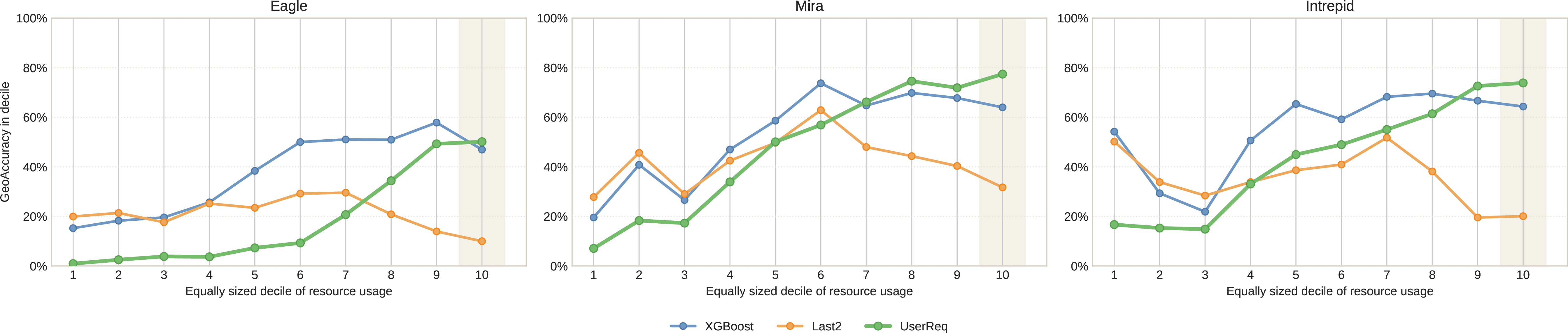
Figure 5 shows the decile pattern behind the changed offline conclusion. UserReq is not uniformly strong across the workload. In the lowest deciles of resource usage, it is often the weakest
of the three methods because many small jobs are requested conservatively and therefore look inaccurate under a multiplicative metric. This pattern changes sharply as resource usage increases.
From the first to the tenth decile of resource usage, UserReq GeoAccuracy rises from 0.009 to 0.501 in Eagle, from 0.071 to 0.774 in Mira, and from 0.167 to 0.738 in Intrepid. By the upper tail,
UserReq closes the gap with XGBoost and becomes stronger in the region with the highest resource usage: the tenth decile in Eagle, the seventh through tenth deciles in Mira, and the ninth and tenth
deciles in Intrepid.
This decile shift explains why GeoAccuracy and MeanAccuracy support different offline conclusions. MeanAccuracy gives equal weight to the many jobs with low resource usage where UserReq is weak. GeoAccuracy gives much more weight to the
upper deciles, where UserReq becomes progressively more accurate and where resource usage is concentrated. The overall metric difference is therefore driven by a clear change in predictor behavior across deciles.
4.3 Top Decile Results Localize the Advantage Relevant to Scheduling↩︎
Figure 5 already shows the decile trend. The highest decile localizes the advantage relevant to scheduling because it is the part of the workload that carries most of the resource usage.
| Dataset | Model | |||
| usage | ||||
| GeoAccuracy | ||||
| \(\mathrm{UnderRate}\) | ||||
| Eagle | XGBoost | 86.5% | 0.470 | 72.7% |
| Last2 | 0.100 | 82.5% | ||
| UserReq | 0.501 | 34.1% | ||
| Mira | XGBoost | 82.3% | 0.640 | 77.9% |
| Last2 | 0.317 | 74.0% | ||
| UserReq | 0.774 | 32.2% | ||
| Intrepid | XGBoost | 81.4% | 0.643 | 75.7% |
| Last2 | 0.201 | 80.3% | ||
| UserReq | 0.738 | 26.0% |
7pt
Table 2 reports the exact metrics for the top decile. In every dataset, UserReq achieves the highest GeoAccuracy in the top decile and the lowest underestimation rate. Relative to
XGBoost, its GeoAccuracy in the top decile rises from 0.470 to 0.501 in Eagle, from 0.640 to 0.774 in Mira, and from 0.643 to 0.738 in Intrepid. Over the same datasets, UnderRate falls from 72.7% to
34.1%, from 77.9% to 32.2%, and from 75.7% to 26.0%, which corresponds to reductions of 38.6, 45.7, and 49.7 percentage points, respectively. It is also the only method that performs best on both GeoAccuracy and UnderRate in the top decile on all three
datasets.
Across datasets, XGBoost remains competitive on GeoAccuracy in the tail, but its underestimation rate stays much higher; Last2 is weaker on both tail metrics. This pattern across datasets is already clear from the reported
values.
Taken together, these top decile results show a consistent pattern in the upper tail with clear implications for scheduling. The same prediction source that looks weak on many small jobs becomes both more accurate and less prone to underestimation on the jobs that dominate resource usage. That is the direct offline signal behind the hybrid policy studied later: if one prediction source is simultaneously safer and more accurate in the upper tail that matters most for scheduling, then routing that tail differently becomes a natural online design choice.
4.4 Results at the Split Level Show That the Signal Is Stable↩︎
Following the protocol at the split level in Section 3, we treat each rolling split day as one analysis unit and compare XGBoost with UserReq only on the split days where both predictors have valid offline metrics. Table 3 reports the resulting win rates across split days. The signal at the split level remains stable under both metrics, but its direction depends on the metric: \(A_{\mathrm{mean}}\)
usually favors XGBoost, whereas \(A_{\mathrm{geo}}\) usually favors UserReq. XGBoost has the higher \(A_{\mathrm{mean}}\) on 67.3%–87.4% of split days,
while UserReq has the higher \(A_{\mathrm{geo}}\) on 68.9%–81.0% of split days. The reversal at the split level is therefore not coming from a few isolated days; it is the dominant direction across the rolling
sequence.
| Dataset | |||
| \(A_{\mathrm{mean}}\) | |||
| \(A_{\mathrm{geo}}\) | |||
| \(\mathrm{UnderRate}\) | |||
| Eagle | 87.3% | 68.9% | 97.4% |
| Mira | 67.3% | 81.0% | 98.9% |
| Intrepid | 87.4% | 79.1% | 99.6% |
UserReq’s advantage on underestimation is even more stable. It achieves the lower UnderRate in 97.4% of split days on Eagle, 98.9% on Mira, and 99.6% on Intrepid. Variation at the split level is still
expected because each day has a different test set size and a different upper tail composition. Even so, the dominant direction is consistent across the rolling sequence. The clearer differentiation under GeoAccuracy, together with UserReq’s
much lower underestimation rate, is therefore a stable effect at the workload level rather than an artifact of a few extreme days.
5 Online Simulation↩︎
The offline results show that UserReq becomes stronger precisely in the part of the workload that dominates resource usage and therefore matters most for scheduling. This section turns that finding into an online test: Section 5.1 defines
the hybrid scheduling policy, Section 5.2 describes the replay setup, and Section 5.3 reports the resulting behavior at the queue level.
5.1 Hybrid Scheduling Policy↩︎
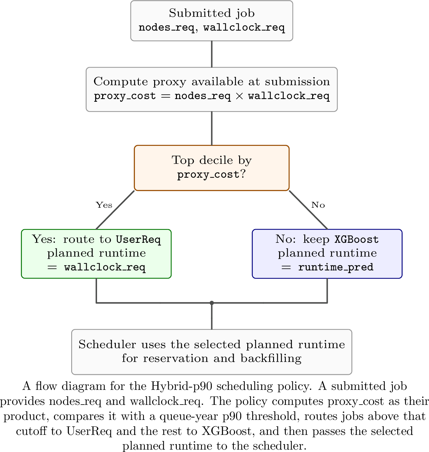
The hybrid policy applies UserReq only to jobs with high values of a proxy for resource usage available at submission. We use \[\texttt{proxy\_cost} = \texttt{nodes\_req} \times \texttt{wallclock\_req}.\]
Under Hybrid-p90, jobs above a p90 cutoff for each queue and year in proxy_cost go to UserReq, and all others stay on XGBoost. This policy does not assume that UserReq should replace machine
learning predictors everywhere. It tests whether routing the tail of jobs with high proxy_cost to UserReq improves scheduling outcomes in online simulation. The p90 choice is intended as a simple, interpretable operating point
motivated by the offline results rather than a claim of global optimality. Figure 6 summarizes the routing rule.
5.2 Online Simulation Setup↩︎
To test the implications of the offline results for scheduling, we supplement the offline evaluation with online replay on Mira and Intrepid. We replay each queue and year partition independently, for example
Mira/prod-short/2016. In this replay, the simulator preserves the original job chronology in timestamp order and changes only the planned runtime presented to the scheduler. Each job keeps its trace submit time and requested node count. The
predictor under test supplies the planned runtime seen by the scheduler. For XGBoost, we use the same hyperparameter setting as in the original runtime prediction workflow of Menear et al. [5]. Reservation and backfilling decisions use that planned runtime, while node release uses the actual runtime from the trace.
The online simulation is intentionally simple. Each partition for a queue and year is simulated independently under FCFS with EASY backfilling. At each job submission or completion event, the scheduler first computes the
earliest feasible reservation for the job at the head of the queue. It then scans later queued jobs in submit order and starts any job whose requested nodes and predicted runtime fit without delaying that reservation. Once started, a job occupies its
requested nodes for its actual runtime. Those nodes are returned to the partition when the job completes. Partition capacity is inferred from the observed peak concurrent node usage in the trace.
To keep the comparison fair, the online simulation is restricted to jobs for which XGBoost, Last2, and UserReq all produce valid predictions after runtime filtering and prediction validity checks. The simulator
reports mean wait time and the count of backfilled jobs.
For the online simulation comparison, we evaluate the hybrid routing policy defined above rather than treating the offline result as only a comparison at the model level. The online simulation summary reports the relative change in mean wait time and
the count of backfilled jobs across four queues drawn from the long and short production queues on Mira and Intrepid. We focus on these four queues because short and long production queues are common and representative in HPC
operations, and together they expose both short job and long job scheduling regimes on two different systems.
Across these four replay queues, proxy_cost aligns well with the heavy tail region. At the same queue and year granularity used by the hybrid policy, the proxy_cost top decile attains 80.4%–91.2% recall and 88.5%–93.5% recall
weighted by cost with respect to the top decile of real cost. Table 4 summarizes the values for each queue.
| Dataset | Queue | Precision | Recall | |
| Recall | ||||
| Mira | prod-short | 72.9% | 81.4% | 89.8% |
| Mira | prod-long | 57.5% | 91.2% | 93.5% |
| Intrepid | prod-short | 61.1% | 80.4% | 88.5% |
| Intrepid | prod-long | 69.5% | 88.9% | 92.4% |
5.3 Hybrid Replay Validates the Offline Signal↩︎
We test whether the offline signal carries through to outcomes at the queue level on Mira and Intrepid. The hybrid rule routes only jobs with high proxy_cost to UserReq. In the replay,
Hybrid-p90 sends the top decile of jobs by proxy_cost within each partition for a queue and year to UserReq and leaves the rest on XGBoost. Figure 7
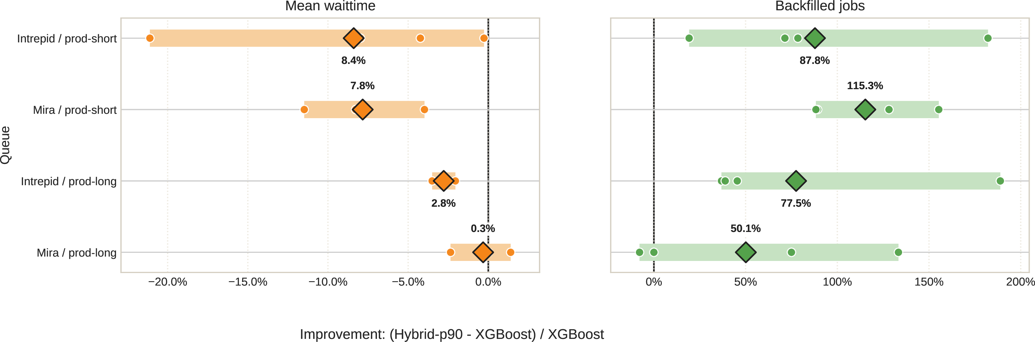
summarizes the comparison across cases in a single view. For each of four queues, the diamond and its adjacent label mark the average relative change across years under \((\texttt{Hybrid-p90} - \texttt{XGBoost}) /
\texttt{XGBoost}\), the pale background bar shows the yearly span, and the smaller points show the individual cases for each queue and year. The yearly cases span 2015–2018 for Mira and 2010–2013 for Intrepid.
Hybrid-p90 improves both metrics in all four cases. In every case, it reduces mean wait time relative to XGBoost and increases the number of backfilled jobs. The clearest gains in wait time appear in the short queues:
Intrepid/prod-short shows an average relative wait reduction of 8.4%, and Mira/prod-short shows a reduction of 7.8%. Intrepid/prod-long still improves by 2.8%, while Mira/prod-long is nearly neutral at
0.3% lower average wait because one later year offsets earlier gains.
The backfilling side is even more uniformly favorable. The gains in short queues are especially large: 115.3% in Mira/prod-short and 87.8% in Intrepid/prod-short. The gains in long queues are also substantial. They reach 77.5%
in Intrepid/prod-long and 50.1% in Mira/prod-long. These percentages should be interpreted directionally rather than as throughput multipliers, because the baseline number of backfilled jobs is small in some long queue years. Even
with that caveat, the figure shows a clear and repeatable effect at the queue level: routing based on proxy_cost tends to preserve more backfill opportunities while also shortening wait time. This pattern suggests that the short production
queues leave more room for backfill gains in our replay, a result that is consistent with prior studies that characterize workloads [6].
The points for each year in Figure 7 show that the average diamonds are not driven by a single anomalous year. The short queues on both systems, together with Intrepid/prod-long, improve
in every simulated year on both mean wait time and the count of backfilled jobs. The only mixed case is Mira/prod-long: 2016 and 2017 improve on both metrics, 2018 is slightly worse on both, and 2015 is effectively tied because both policies
backfill the same small number of jobs. The dot range summary therefore preserves the yearly pattern directly instead of hiding instability behind a single average.
These results link the offline tail effect to scheduling outcomes. A simple policy at submission time that invokes UserReq only on jobs with high proxy_cost improves both mean wait time and backfilling in all four queues. The
simulation is intentionally limited: it uses partitions for each queue and year with FCFS scheduling and EASY backfilling rather than a production scheduler deployment. We therefore interpret the result as evidence of scheduling
impact rather than full scheduler validation.
6 Related Work↩︎
We place this paper in the context of three adjacent areas: runtime prediction methods, studies of user provided walltime estimates and backfilling, and work that evaluates prediction quality through scheduling outcomes. This paper is closest to the third area because it asks how runtime predictors should be evaluated, rather than proposing a new predictor.
6.1 HPC Runtime Prediction↩︎
HPC job runtime prediction has a long history spanning models based on historical information, predictors based on logs, and more recent machine learning systems. Early work showed that historical behavior can support scheduling decisions [11], and later studies used system logs or job attributes to predict completion time more directly [12], [13]. Recent work has focused largely on
improving the predictor itself through ensemble methods, deep learning, feature engineering, or domain specific and two step estimation strategies [5], [10], [14]–[16]. Among these, tree ensemble methods such as XGBoost [9] are especially common because they handle heterogeneous submission features and nonlinear interactions well, and they have become strong
practical baselines in HPC runtime prediction studies [5], [10]. In this literature, performance is usually summarized with aggregate arithmetic mean metrics such as RMSE, MAE, or overall accuracy like scores, sometimes together with risk measures focused on underestimation [17].
A related but distinct line of work studies predictive uncertainty through conditional quantiles and prediction intervals. Large scale quantile regression makes quantile estimation practical on very large datasets [18], and conformalized quantile regression adds prediction intervals that are valid for finite samples [19]. These methods target uncertainty quantification, not evaluation oriented toward schedulers under resource usage with heavy tails.
Our question is different from both predictor construction and interval estimation. We reevaluate existing prediction sources under different aggregation rules. Under resource usage with heavy tails, the choice of metric can reveal clearer differences among predictors and therefore support different conclusions about their quality for scheduling. The focus is therefore on predictor evaluation rather than predictor construction.
6.2 User Provided Runtime Estimates and Backfilling↩︎
User provided runtime estimates have been studied for decades because they affect reservation length, backfilling opportunities, and queue performance directly. Much of this literature emphasizes that user estimates are systematically overestimated or
otherwise inaccurate in aggregate [20], [21]. However, the same line of work also shows that their operational value should not be dismissed: under EASY backfilling, conservative user estimates can preserve reservation safety and may even help
utilization or queue behavior in some settings [2], [22]–[24]. Subsequent
work studied adjusted user estimates, controls for underestimation, and scheduler mechanisms that replace or augment user estimates with predictions generated by the system [4], [17], [25]–[28]. Runtime prediction has also been linked
to queue time prediction and scheduler performance more broadly [3], [29]–[31].
Our results complement this literature. We do not claim that user estimates are the most useful prediction source across the whole workload. Instead, we show that they become especially valuable on the upper tail of resource usage and that this effect becomes visible only under evaluation focused on the tail.
6.3 Evaluation Metrics and Scheduling Impact↩︎
Prior work has argued that prediction quality should ultimately be judged by its effect on scheduling rather than by offline accuracy alone [3], [32], [33]. Trace studies also show that large HPC workloads are heterogeneous and that aggregate averages can hide important structural differences across jobs, users, and resource classes [6], [34], [35]. At the same time, most runtime prediction papers still treat the evaluation metric as fixed and place the novelty in the predictor.
Relative to that evaluation oriented line of work, this paper combines three elements. First, it uses an overall metric, \(A_{\mathrm{geo}}\), that weights error by resource usage alongside the metric based on averaging over jobs, \(A_{\mathrm{mean}}\). Second, it uses equally sized deciles of resource usage to explain why GeoAccuracy reveals clearer differences among the methods. Third, it uses online replay to test whether those offline differences translate into scheduling outcomes. We are not aware of prior HPC runtime prediction work that centers this combination of evaluation focused on the tail, explanation at the decile level, and validation at the queue level, while explicitly linking the offline metric choice to the upper tail of the workload that matters most for scheduling.
7 Conclusion↩︎
This paper makes three contributions. First, it presents an empirical evaluation methodology for HPC job runtime prediction that focuses on the tail and combines GeoAccuracy weighted by resource usage with analyses at the decile and split levels.
Second, it shows on three production HPC workloads that evaluation focused on the tail changes the offline conclusion. \(A_{\mathrm{mean}}\) keeps the compared methods relatively close, whereas \(A_{\mathrm{geo}}\) reveals clearer separation and makes UserReq’s strength in the resource dominant upper tail visible. In the top decile, UserReq achieves the highest GeoAccuracy and the lowest
underestimation rate on all three datasets, and this advantage remains stable across rolling split days.
Third, it translates this offline signal into a simple hybrid scheduling policy and shows in online replay that it improves scheduling performance. This policy uses proxy_cost at submission as the routing rule. It keeps XGBoost
for most jobs and routes the top decile to UserReq. Across the short and long production queues on two HPC systems, it reduces mean wait time by up to 8% and increases backfilled jobs by 50%–115%.
These results indicate that offline evaluation focused on the tail should inform the assessment of runtime predictors and scheduling policy design under HPC workloads with heavy tails. They also suggest that no single prediction source serves the entire workload equally well: machine learning predictors remain useful on the bulk of jobs, while the user provided walltime estimate at job submission carries valuable signal in the upper tail. Online schedulers should therefore combine multiple prediction signals through a hybrid policy rather than forcing one source to serve the whole workload.