When Do Foundation Models Pay Off?
A Break-Even Analysis of Pretrained Time Series Forecasters
July 06, 2026
Abstract
Deploying a time series foundation model requires GPU infrastructure, engineering overhead, and carries no guarantee of improvement over XGBoost. We provide the first systematic break-even analysis answering when this investment pays off. Across 30 benchmark datasets, we compare zero-shot and LoRA fine-tuned foundation models (Chronos, Moirai, Lag-Llama) against classical baselines (Naive, ETS, ARIMA, XGBoost) at six training set sizes from 2% to 100% of available data. Foundation models outperform classical methods at every evaluated training fraction on 15 of 30 datasets—GPU deployment is unconditionally justified on these regardless of data volume. On 6 datasets, classical methods surpass zero-shot foundation models with as little as 2% of training data (21–2,768 samples); on the remaining 9, break-even ranges from 24 to 8,361 samples. One robust deployment rule requires no model training: if \(n_{\text{train}} < 700\) and seasonality is non-negligible, use FM zero-shot and skip fine-tuning—this resolves 10 of 30 deployment decisions immediately. Contrary to common practice, LoRA fine-tuning can actively degrade performance on short series. We operationalise these findings as a two-step decision framework—compute dataset length and seasonality strength, run a brief 5–10% pilot only if needed—enabling practitioners to make the FM-versus-classical decision before committing to full infrastructure. Four dataset features motivate mechanistic hypotheses for the remaining cases, though reliable automated prediction at this benchmark scale remains an open problem. Code, benchmark, and decision tools are available at https://github.com/nicolaisi/fm-breakeven.
time series forecasting, foundation models, model selection, scaling laws, pretrained models
1 Introduction↩︎
The landscape of time series forecasting is undergoing a paradigm shift. Foundation models—large neural networks pretrained on diverse time series corpora—promise to deliver accurate forecasts without task-specific training. Models like Chronos [1], Moirai [2], and Lag-Llama [3] have demonstrated impressive zero-shot performance across benchmarks, leading to widespread adoption: the Chronos model family has tens of millions of downloads on Hugging Face across all variants.
Yet practitioners face a fundamental question: Should I use a foundation model, or stick with XGBoost? This seemingly simple question lacks a clear answer. Foundation models require GPU infrastructure, have opaque failure modes, and may underperform on domain-specific data. Classical methods like exponential smoothing or gradient boosting are interpretable, run on CPUs, and have decades of empirical validation. The right choice depends on factors that are poorly understood. The cost of a wrong choice is asymmetric: deploying a foundation model unnecessarily means GPU infrastructure, latency overhead, and engineering complexity; sticking with XGBoost when a foundation model would dominate means leaving accuracy on the table.
We hypothesize that the comparison between foundation models and classical methods is not static but data-dependent. With limited task data, foundation models may win due to their pretrained representations. With abundant task data, classical methods may catch up or surpass foundation models by learning task-specific patterns. The break-even point—the amount of task data at which classical methods begin outperforming foundation models—likely varies across datasets based on intrinsic properties.
1.1 Research Questions↩︎
We address three questions that together provide theoretical understanding and practical guidance:
RQ1: Break-Even Existence and Variation. Do foundation models consistently outperform classical methods, or does the comparison depend on data volume? If break-even points exist, how much do they vary across datasets?
RQ2: Determinants of Break-Even. What dataset properties influence whether and when foundation models become beneficial? Can we identify features that predict break-even behavior?
RQ3: Practical Decision Support. What can dataset properties reveal about break-even behavior, and are there simple rules practitioners can apply without running experiments? We seek to characterize the limits of such prediction at our benchmark scale and identify any rules that are empirically robust.
1.2 Contributions↩︎
We make three contributions addressing these questions:
1. Systematic Benchmark. We conduct a comprehensive head-to-head comparison across 30 datasets, 6 foundation model variants (evaluated under up to 3 settings each: zero-shot, LoRA fine-tuning, and full fine-tuning), 4 classical baselines, 6 training size fractions, and 3 seeds—totaling 10,800 experimental configurations (\(30 \times 20 \times 6 \times 3\), where the 20 model-settings comprise 16 FM configurations and 4 classical baselines).
2. Break-Even Analysis. We introduce break-even analysis as a framework for foundation model evaluation and identify four dataset categories: FM-dominant (15 of 30), early break-even (classical wins with as little as 2% of data; 6 datasets), mid break-even (1 dataset), and late break-even (classical needs substantial data; 8 datasets). For practical guidance, mid and late break-even collapse into a single “substantial-data-required” regime. Critically, we find that zero-shot foundation models outperform fully-trained classical models on 15 of 30 datasets without any task-specific training—FM-dominant is the plurality category.
3. Mechanistic Feature Hypotheses and a Robust Decision Rule. We identify one empirically robust rule: datasets with \(n_{\text{train}} < 700\) samples and non-negligible seasonality (\(S \geq 0.05\)) consistently favour FM zero-shot. Four dataset features—series length, seasonal strength, noise ratio, and mean autocorrelation—co-vary with break-even patterns and motivate mechanistic hypotheses for each. A random forest classifier on these features achieves 60.0% LOO accuracy under a three-way taxonomy and 53.3% under a four-way taxonomy (both above the 50% majority-class baseline), providing marginal above-chance prediction at this benchmark scale: these hypotheses are testable propositions for future validation on larger benchmarks, not a validated predictive tool.
2 Related Work↩︎
2.1 Time Series Foundation Models↩︎
Foundation models for time series have emerged rapidly since 2023. Chronos [1] reframed time series as a language modeling problem using T5-based models; Chronos-Bolt [1] improved efficiency via direct multi-step patch forecasting. Lag-Llama [3] adopted a decoder-only architecture with lag features. Moirai [2] introduced a universal model handling varying frequencies and prediction lengths. These models are typically evaluated at fixed data sizes; our work examines how their advantage evolves with task data volume.
2.2 Scaling Laws for Time Series↩︎
Scaling laws characterize how model performance improves with data, compute, or model size. Kaplan et al.[4] established power-law scaling for language models.
For time series, Zeng et al.zeng2023transformers? showed that simple linear models can outperform complex transformers on standard benchmarks—a finding that motivates dataset-conditional evaluation. Shi et al.[5] subsequently studied scaling laws within neural architectures, and Edwards et al.[6] studied scaling for transformer-based time series models. Zhou et al.[7] showed that models with as few as 10k parameters can match FM performance on specific tasks.
Our work differs by studying scaling across model paradigms—comparing pretrained foundation models against classical methods that learn only from task data.
2.3 Meta-Learning for Model Selection↩︎
Meta-learning approaches predict model performance from dataset characteristics. Talagala et al.[8] proposed FFORMS, using time series features to select forecasting methods, achieving strong results on the M4 competition. Montero-Manso et al.[9] extended this to model averaging with gradient-boosted meta-learners, achieving top performance in the M4 forecasting competition [10]. Recent work explores online selection [11] and LLM-based selection [12].
Unlike FFORMS/FFORMA, which predict which method is best at full data, we ask at what training volume the ranking changes—reframing selection as a threshold estimation problem that prior work does not address.
2.4 Foundation Model Evaluation↩︎
Benchmarks for foundation models typically report aggregate metrics at full data. Godahewa et al.[13] introduced the Monash archive for standardized evaluation. Xu et al.[14] found that properly tuned supervised baselines remain competitive with specialized foundation models, leaving practitioners without clear guidance on which approach to deploy. Ye et al.ye2024survey? provide a comprehensive survey of large models for time series, covering evaluation methodology and open challenges. Zhou et al.[7] showed that extremely small models can match FM performance on specific tasks, further motivating dataset-conditional evaluation.
We address these concerns by evaluating across 30 datasets spanning diverse domains and frequencies—substantially broader than the 7-dataset ETT-family benchmarks used in prior comparisons—using carefully configured baselines, varying training data volumes, and including gradient boosting, a competitive method often omitted from neural network benchmarks.
3 Methodology↩︎
3.1 Problem Formulation↩︎
Consider a forecasting task with training data \(\mathcal{D}_n = \{(x_t, y_{t+h})\}_{t=1}^{n}\) where \(x_t\) represents historical observations and \(y_{t+h}\) is the target \(h\) steps ahead. Let \(f_{\text{FM}}\) denote a foundation model (potentially fine-tuned on \(\mathcal{D}_n\)) and \(f_{\text{CL}}\) denote a classical method trained on \(\mathcal{D}_n\).
We define the break-even point \(n^*\) as the smallest training set size where the classical method matches or exceeds the best foundation model: \[n^* = \min \{ n : \text{Error}(f_{\text{CL}}, n) \leq \text{Error}(f_{\text{FM}}) \}\] where \(f_{\text{FM}}\) is evaluated in zero-shot mode. If no such \(n\) exists within the available data range, we say \(n^* = 0\) (foundation model always wins, FM-dominant) or \(n^* = \infty\) (classical method always wins even from minimal data). In practice, we observe three main patterns for practical guidance: FM-dominant (\(n^* = 0\)), early break-even (\(n^*\) at 2–5% of data), and late break-even (at 20–100% of data). A mid break-even regime (at \(\approx\)10%) is observed on 1 dataset (Weather) and is subsumed into late for robust guidance; we retain the four-way descriptive split in figures and tables for completeness.
3.2 Scaling Curve Framework↩︎
We characterize the empirical relationship between training data volume and forecast error by evaluating both model families at discrete training fractions and observing how error changes with \(n\).
Foundation models and classical methods exhibit characteristically different scaling behavior in our experiments:
Foundation models produce constant error as a function of \(n\) in zero-shot mode—performance is independent of task data by construction. When fine-tuned via LoRA, error may decrease with \(n\) on datasets with clear periodicity, or increase due to overfitting on short series.
Classical methods start with higher error at low \(n\) but generally improve as more task-specific data becomes available. Their asymptotic performance depends on how well the dataset’s structure can be captured by the model family.
The break-even point \(n^*\) is where the classical error curve falls below the FM zero-shot baseline. If FM curves remain below classical at all evaluated fractions, \(n^* = 0\) (FM-dominant). If the classical curve never falls below FM zero-shot within the evaluated range, no finite \(n^*\) exists and the dataset is classified FM-dominant; the \(n^* = \infty\) case (classical always wins even at minimal data) is not observed in our benchmark. We determine break-even empirically from the discrete fraction grid rather than by fitting parametric curves, which avoids extrapolation artefacts on small datasets. We partition datasets into four categories based on the smallest training fraction at which any classical method first matches or beats FM zero-shot: FM-dominant (no break-even observed), Early (\(\leq\)5% of data), Mid (10%), and Late (\(\geq\)20%). The Mid category corresponds to a single grid point (10%) between the Early and Late thresholds.
3.3 Dataset Selection↩︎
We select 30 benchmark datasets spanning diverse domains, frequencies, and characteristics. Table 1 summarizes dataset properties.
| Dataset | Domain | Freq. | Length | Vars | Horizon |
|---|---|---|---|---|---|
| Dominick | Retail | 1W | 90 | 1 | 8 |
| Hospital | Health | ME | 84 | 1 | 12 |
| M4-Monthly-Monash | Mixed | ME | 78 | 1 | 18 |
| M3-Monthly | Mixed | ME | 83 | 1 | 18 |
| M3-Quarterly | Mixed | QE | 44 | 1 | 8 |
| Tourism-Monthly | Tourism | ME | 243 | 1 | 24 |
| COVID-Deaths | Health | 1D | 212 | 1 | 30 |
| M4-Daily | Mixed | 1D | 379 | 1 | 14 |
| M4-Weekly | Mixed | 1W | 379 | 1 | 13 |
| Rideshare | Transport | 1H | 541 | 1 | 24 |
| ILI | Health | 1W | 966 | 7 | 24 |
| M4-Hourly | Mixed | 1H | 700 | 1 | 24 |
| FRED-MD | Economics | ME | 728 | 1 | 12 |
| NN5-Daily | Finance | 1D | 791 | 1 | 56 |
| USBirths | Health | 1D | 7,305 | 1 | 30 |
| Exchange | Finance | 1D | 7,588 | 8 | 30 |
| KDD-Cup-Hourly | Air Qual. | 1H | 10,898 | 1 | 48 |
| ETTh1 | Energy | 1H | 17,420 | 7 | 24 |
| ETTh2 | Energy | 1H | 17,420 | 7 | 24 |
| Traffic | Transport | 1H | 17,544 | 862 | 24 |
| Pedestrian | Transport | 1H | 22,259 | 1 | 24 |
| Saugeen | Hydrology | 1D | 23,741 | 1 | 30 |
| Electricity | Utilities | 1H | 26,304 | 321 | 24 |
| Weather | Climate | 10min | 52,696 | 21 | 720 |
| Solar-10min | Energy | 10min | 52,560 | 1 | 60 |
| ETTm1 | Energy | 15min | 69,680 | 7 | 96 |
| ETTm2 | Energy | 15min | 69,680 | 7 | 96 |
| Sunspot | Science | 1D | 73,924 | 1 | 30 |
| AusElectricity | Utilities | 30min | 230,736 | 1 | 48 |
| Wind-Farms | Energy | 1min | 527,040 | 1 | 60 |
3pt
All experiments use univariate forecasting (OT target column). Lengths shown are after multi-series aggregation; see Section [sec:sec:datasets] for
competition dataset truncation details.
Selection criteria include: (1) public availability for reproducibility, (2) domain diversity spanning energy, transport, finance, health, and climate, (3) sufficient length to enable meaningful subsampling, and (4) prior use in forecasting benchmarks. For competition datasets (M3, M4) containing collections of variable-length series, we truncate each series to the 25th percentile of collection lengths prior to subsampling, ensuring that reported training fractions correspond to lengths achievable by the majority of series in the dataset. One dataset required additional preprocessing: the Rideshare series (averaged across multiple vehicles in the Monash collection) contained a constant-valued suffix of \(\approx\)200 timesteps arising from COVID-era zero-rideshare padding in the original data. This suffix was identified and removed prior to the train/test split; without this step, classical models predict a constant, making MASE dominated by the seasonal-naïve denominator rather than forecast quality.
3.4 Model Selection↩︎
3.4.1 Foundation Models↩︎
We evaluate six foundation model variants spanning three model families:
Chronos family [1]: Chronos-Bolt Small (48M parameters) and Chronos-Bolt Base (205M). These use a patch-based T5 architecture with direct multi-step forecasting and a built-in quantile loss for supervised fine-tuning.
Moirai family [2]: Moirai-Small (14M), Moirai-Base (91M), and Moirai-Large (311M). These use an encoder-only transformer with mixture distribution outputs and support fine-tuning via the MoiraiFinetune interface.
Lag-Llama [3]: A 7M parameter decoder-only model using lag features for probabilistic forecasting. Evaluated in zero-shot mode only, as its GluonTS-based training loop does not expose a compatible interface for LoRA adapter injection without substantial modification to the checkpoint loading pipeline.
For Chronos and Moirai, we evaluate three settings: zero-shot (direct inference without task-specific training), full fine-tuning (updating all pretrained weights on task data), and LoRA fine-tuning [15] (rank-8 adapters, freezing backbone weights). Lag-Llama is evaluated zero-shot only. Full fine-tuning results (updating all weights) are collected but omitted from main tables due to instability (see Limitations); LoRA is the reported fine-tuning setting for Chronos and Moirai.
3.4.2 Classical Baselines↩︎
We include four classical methods representing different paradigms:
Naive: Seasonal naive baseline repeating the last observed seasonal cycle. Despite simplicity, this is often competitive for highly seasonal data.
ETS: Exponential smoothing with automatic model selection [16].
ARIMA: Auto-ARIMA with automatic order selection [16]. Searches over ARIMA\((p,d,q)\) and seasonal variants.
XGBoost: Gradient boosting with lag features [17]. We create features from lagged values, calendar indicators, and rolling statistics. This represents modern machine learning approaches competitive on tabular data.
3.5 Experimental Protocol↩︎
3.5.1 Training Size Variation↩︎
For each dataset, we create training sets at six logarithmically-spaced fractions: 2%, 5%, 10%, 20%, 50%, and 100% of available training data. Subsampling preserves temporal order by taking the most recent fraction, mimicking realistic scenarios with limited historical data. For very short datasets (ILI, M4-Hourly, and several competition series with \(n_{\text{train}}<100\): Hospital, M3-Monthly, M3-Quarterly, Dominick), the smallest fractions yield fewer than 50 samples, which is below the minimum required for reliable classical model fitting (particularly ARIMA). These configurations are excluded from classical results and noted in the analysis.
FM context window. Foundation models always receive the full historical series as context; classical methods are restricted to the current training fraction. FM error curves are thus horizontal by construction.
3.5.2 Evaluation Protocol↩︎
Models are trained on each subsample and evaluated on held-out test sets (the final 20% of data, chronologically ordered). All datasets use a chronological 60/20/20 split: the first 60% is the training pool, the middle 20% acts as a temporal buffer (not used for model training or selection), and the final 20% is the held-out test set. We repeat experiments with three random seeds to estimate variance.
3.5.3 Metrics↩︎
Our primary metric is Mean Absolute Scaled Error (MASE) [18]. Important: to ensure comparability across training fractions, \(T\) in the denominator is always fixed to the full training set (\(\text{frac}=1.0\)) rather than the current fraction; only the numerator (forecast error) varies across fractions. The seasonal period \(m\) is set per-dataset: \(m=24\) for hourly datasets (ETTh1/2, Electricity, Traffic, M4-Hourly), \(m=96\) for 15-minute datasets (ETTm1/2), \(m=144\) for 10-minute Weather, \(m=52\) for weekly ILI, and \(m=5\) for daily Exchange. Exchange denominator caveat: Exchange has \(S=0.00\) and no meaningful seasonal period; its MASE (\(\approx\)8–9) partly reflects the arbitrary \(m=5\) denominator and should not be directly compared across datasets.
Seed variance. Table 2 reports the minimum MASE over three independent seeds per model; Table 3 reports means over seeds and 30 datasets. For FM zero-shot models at \(\text{frac}=1.0\), seed standard deviations of the best model per dataset average 0.028 (median 0.007); most datasets have seed std below 0.10, with M4-Hourly (Lag-Llama, std=0.277) the notable outlier—consistent with its narrow FM–classical margin and its inclusion in the Table 2 caution list. Classical methods are deterministic given fixed data, seed std \(\approx 0\). LoRA fine-tuning seed std averages 0.095 at low fractions (\(\leq\)5%, max 2.58) and 0.164 at full data; full fine-tuning is higher still at low fractions (mean 0.129), consistent with LoRA being the more stable fine-tuning default in the low-data regime. Full seed-level MASE values are provided in the repository.
3.5.4 Computational Setup and Reproducibility↩︎
Experiments run on a workstation with an NVIDIA RTX 5090 GPU (32 GB DDR7 VRAM). Foundation model inference and fine-tuning use GPU; classical methods use CPU. Total GPU compute time for all FM experiments was approximately 8 GPU-hours (Chronos/Moirai across 30 datasets \(\approx\)7.5 hours, Lag-Llama \(\approx\)25 minutes); classical experiments ran on CPU in parallel.
LoRA configuration. For Chronos, adapters target q and v projections (\(r=8\), \(\alpha=16\), dropout=0.05). For Moirai, adapters target
q_proj, k_proj, v_proj, out_proj (same hyperparameters). Both use AdamW (\(\text{lr}=10^{-4}\), weight decay 0.01), with training steps \(\min(300, \max(50, \lfloor n/H \rfloor))\).
XGBoost uses lags up to \(\min(2m, 48)\), rolling mean/std at windows \(\{m/2, m, 2m\}\), and calendar indicators (n_estimators=100,
max_depth=6, lr=0.1).
Code and data. All feature extraction, experiment scripts, and analysis code are released at https://github.com/nicolaisi/fm-breakeven. Datasets are publicly available from their original sources; download links and preprocessing scripts are included in the repository.
3.6 Dataset Feature Extraction↩︎
We extract six features capturing intrinsic data properties that may influence break-even behavior. All features are computed from training data without model fitting.
ACF decay lag (\(\tau_{\text{acf}}\)): The lag at which the autocorrelation function first falls below 0.5, measuring how quickly temporal memory decays. Reported in Table 4 for reference but capped at 200 for long-memory series, limiting its discriminative power.
Mean absolute autocorrelation (\(\overline{|\rho|}_{50}\)): The mean of \(|\rho(k)|\) for \(k = 1, \ldots, 50\), measuring sustained temporal memory without saturation. Used in the classifier as the unsaturated replacement for \(\tau_{\text{acf}}\).
Hurst exponent (\(H\)): Estimated via detrended fluctuation analysis (DFA), measuring long-range dependence without the saturation artefacts of classical R/S analysis. \(H = 0.5\) indicates no memory; \(H > 0.5\) indicates persistence.
Noise ratio (\(\sigma_r\)): Ratio of differenced to original standard deviation: \[\sigma_r = \frac{\text{std}(x_t - x_{t-1})}{\text{std}(x_t)}\] Higher values indicate noisier series dominated by innovations.
Seasonal strength (\(S\)): From STL decomposition: \[S = 1 - \frac{\text{Var}(R)}{\text{Var}(Y - T)}\] where \(R\) is the remainder and \(T\) is the trend component.
Spectral entropy (\(\Phi\)): Entropy of the normalized periodogram, measuring predictability. Low \(\Phi\) indicates concentrated spectral power (predictable); high \(\Phi\) indicates diffuse power (unpredictable).
Feature extraction completes in under one minute per dataset.
4 Results↩︎
4.1 Scaling Curves and Break-Even Points (RQ1)↩︎
Figure 1 shows scaling curves for all 30 datasets. We observe four distinct patterns:
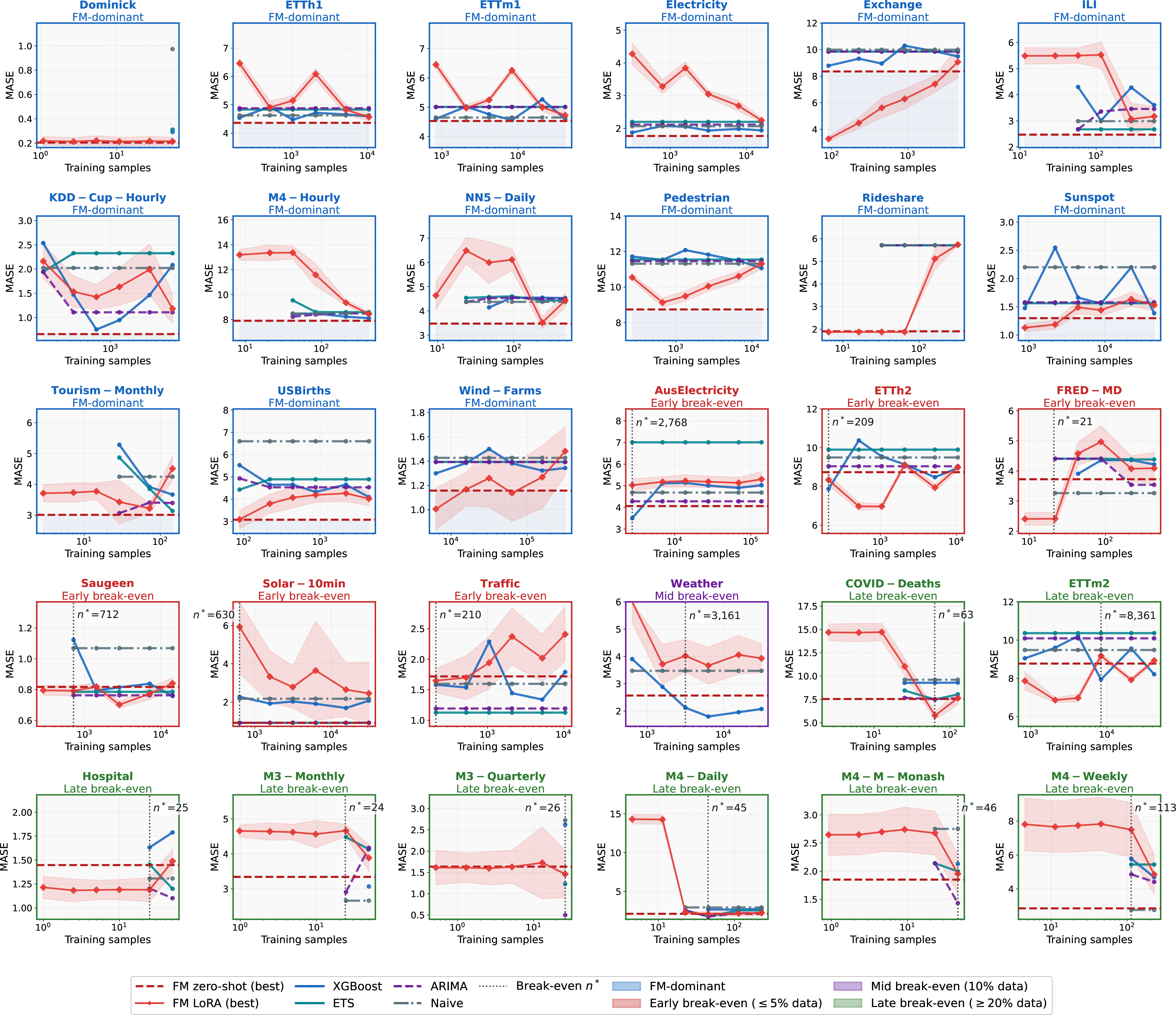
Pattern 1: FM-Dominant. On 15 datasets (Dominick, ETTh1, ETTm1, Electricity, Exchange, ILI, KDD-Cup-Hourly, M4-Hourly, NN5-Daily, Pedestrian, Rideshare, Sunspot, Tourism-Monthly, USBirths, Wind-Farms), the best foundation model (zero-shot) outperforms the best classical method at every evaluated training fraction. ETTm1 (\(\Delta=0.066\)) and ETTh1 (\(\Delta=0.229\)) have the smallest margins among long-series datasets; several others (Dominick \(\Delta=0.008\), Sunspot \(\Delta=0.087\), M4-Hourly \(\Delta=0.210\), Tourism-Monthly \(\Delta=0.126\), Wind-Farms \(\Delta=0.186\), Electricity \(\Delta=0.171\), ILI \(\Delta=0.203\)) also have gaps below 0.3 MASE and should be confirmed with additional seeds (see Table 2 footnote).
Pattern 2: Early Break-Even. On 6 datasets (AusElectricity, ETTh2, FRED-MD, Saugeen, Solar-10min, Traffic), classical methods surpass zero-shot foundation models with as little as 2% of training data (21–2,768 samples). For FRED-MD, Saugeen, Solar-10min, and Traffic, classical maintains its advantage through 100% training data. For AusElectricity and ETTh2, the crossing is non-monotonic: classical beats FM at 2% but FM regains the lead at 100% training data.
Pattern 3: Mid Break-Even. On 1 dataset (Weather), classical methods require \(\approx\)10% of training data (\(n^* = 3{,}161\) samples).
Pattern 4: Late Break-Even. On 8 datasets (COVID-Deaths, ETTm2, Hospital, M3-Monthly, M3-Quarterly, M4-Daily, M4-Monthly-Monash, M4-Weekly), classical methods require 20–100% of training data (24–8,361 samples) to surpass zero-shot foundation models. With limited or structurally complex data, foundation model pretraining provides substantial benefit.
Table 2 reports break-even points for all datasets.
| Dataset | Best FM (ZS) | MASE | Best CL | MASE | \(n^*\) | Pattern |
|---|---|---|---|---|---|---|
| Dominick | Moirai-S | 0.205 | ARIMA | 0.213 | — | FM-dom. |
| ETTh1 | Moirai-B | 4.362 | XGBoost | 4.591 | — | FM-dom. |
| ETTm1 | Moirai-L | 4.530 | XGBoost | 4.596 | — | FM-dom. |
| Electricity | Moirai-B | 1.768 | XGBoost | 1.939 | — | FM-dom. |
| Exchange | Moirai-L | 8.356 | XGBoost | 9.488 | — | FM-dom. |
| ILI | Chr-Bolt-S | 2.472 | ETS | 2.675 | — | FM-dom. |
| KDD-Cup-Hourly | Chr-Bolt-B | 0.659 | ARIMA | 1.108 | — | FM-dom. |
| M4-Hourly | Lag-Llama | 7.906 | XGBoost | 8.116 | — | FM-dom. |
| NN5-Daily | Lag-Llama | 3.477 | Naive | 4.371 | — | FM-dom. |
| Pedestrian | Lag-Llama | 8.740 | XGBoost | 11.068 | — | FM-dom. |
| Rideshare | Lag-Llama | 1.907 | XGBoost | 5.708 | — | FM-dom. |
| Sunspot | Lag-Llama | 1.298 | XGBoost | 1.385 | — | FM-dom. |
| Tourism-Monthly | Chr-Bolt-B | 3.010 | ETS | 3.136 | — | FM-dom. |
| USBirths | Lag-Llama | 3.074 | XGBoost | 4.091 | — | FM-dom. |
| Wind-Farms | Chr-Bolt-B | 1.157 | XGBoost | 1.343 | — | FM-dom. |
| AusElectricity | Lag-Llama | 4.062 | ARIMA | 4.282 | 2,768 | Early |
| ETTh2 | Moirai-L | 8.732 | XGBoost | 8.948 | 209 | Early |
| FRED-MD | Moirai-S | 3.724 | Naive | 3.263 | 21 | Early |
| Saugeen | Chr-Bolt-B | 0.817 | XGBoost | 0.758 | 712 | Early |
| Solar-10min | Moirai-B | 0.924 | ARIMA | 0.922 | 630 | Early |
| Traffic | Moirai-S | 1.719 | ETS | 1.126 | 210 | Early |
| Weather | Lag-Llama | 2.568 | XGBoost | 2.076 | 3,161 | Mid |
| COVID-Deaths | Moirai-S | 7.547 | ARIMA | 7.613 | 63 | Late |
| ETTm2 | Lag-Llama | 8.771 | XGBoost | 8.211 | 8,361 | Late |
| Hospital | Chr-Bolt-B | 1.448 | ARIMA | 1.101 | 25 | Late |
| M3-Monthly | Lag-Llama | 3.341 | Naive | 2.661 | 24 | Late |
| M3-Quarterly | Chr-Bolt-B | 1.637 | ARIMA | 0.498 | 26 | Late |
| M4-Daily | Chr-Bolt-S | 2.103 | ARIMA | 2.210 | 45 | Late |
| M4-Monthly-M. | Moirai-L | 1.850 | ARIMA | 1.432 | 46 | Late |
| M4-Weekly | Chr-Bolt-S | 2.850 | Naive | 2.758 | 113 | Late |
3pt
ZS = zero-shot. Chr-Bolt = Chronos-Bolt. FM MASE = min over 3 seeds; classical is deterministic. \(n^*\) = first fraction where classical beats FM zero-shot. FM-dom. = FM-dominant. M4-Monthly-M. = M4-Monthly-Monash.
Datasets with FM–classical gap \(<\)0.3 MASE may be reversed with additional seeds: Dominick (\(\Delta=0.008\)), ETTm1 (\(\Delta=0.066\)), Sunspot (\(\Delta=0.087\)), Tourism-Monthly (\(\Delta=0.126\)), Wind-Farms (\(\Delta=0.186\)), Electricity (\(\Delta=0.171\)), ILI (\(\Delta=0.203\)), ETTh1 (\(\Delta=0.229\)), M4-Hourly (\(\Delta=0.210\)).
Key finding: Zero-shot foundation models outperform classical methods at every training fraction on 15 of 30 datasets—FM-dominant is now the plurality category. On 6 datasets, classical methods need only 2% of available data to catch up (21–2,768 samples). The remaining 9 datasets show mid or late break-even behavior. This four-way taxonomy reveals that the FM vs.classical comparison is fundamentally dataset-dependent.
4.2 Model and Setting Analysis↩︎
Table 3 compares foundation model variants and settings.
| Model | Setting | Mean MASE | Best on \(k\) datasets |
|---|---|---|---|
| Chronos-Bolt-S | Zero-shot | 4.11 | 2 |
| LoRA FT | 4.04 | 7 | |
| Chronos-Bolt-B | Zero-shot | 4.13 | 2 |
| LoRA FT | 4.11 | 3 | |
| Moirai-S | Zero-shot | 4.25 | 0 |
| LoRA FT | 4.38 | 2 | |
| Moirai-B | Zero-shot | 4.25 | 1 |
| LoRA FT | 4.40 | 2 | |
| Moirai-L | Zero-shot | 4.27 | 0 |
| LoRA FT | 4.27 | 3 | |
| Lag-Llama | Zero-shot | 5.20 | 8 |
| XGBoost | Trained | 4.20 | 14 |
| ETS | Trained | 4.53 | 3 |
| ARIMA | Trained | 4.75 | 9 |
| Naive | Trained | 4.39 | 4 |
Mean MASE at 100% training data across 30 datasets (means over 3 seeds). Rows are sorted within FM families by parameter count. Among classical methods, XGBoost is listed first as it achieves best performance on the most datasets (14 of 30);
remaining classical rows are not sorted by Best on \(k\). Note on mean MASE: mean MASE is dominated by a small number of high-MASE datasets (ETTh2, ETTm2, Exchange, M4-Hourly, Pedestrian; MASE \(\approx\)8–11) and does not reflect typical-case performance; rankings based on it should be treated with caution. The “Best on \(k\) datasets” column (number of datasets where this model
achieves the lowest MASE within its class: FM models compete among all FM ZS/LoRA variants; classical models compete among the four classical baselines) is the recommended ranking criterion. Note: Moirai-S LoRA FT (4.38) is worse than Moirai-S ZS (4.25) on
aggregate, consistent with LoRA degrading performance on short-series-dominated subsets.
Finding 1: Zero-shot is already competitive. Foundation models in zero-shot mode achieve lower MASE than fully-trained classical methods on 19 of 30 datasets, including the 15 FM-dominant cases where no classical method beats FM zero-shot at any evaluated training fraction. Note that \(n^*\) values in Table 2 are based on the best FM and classical method per dataset; a practitioner committed to a single FM family will typically see higher \(n^*\).
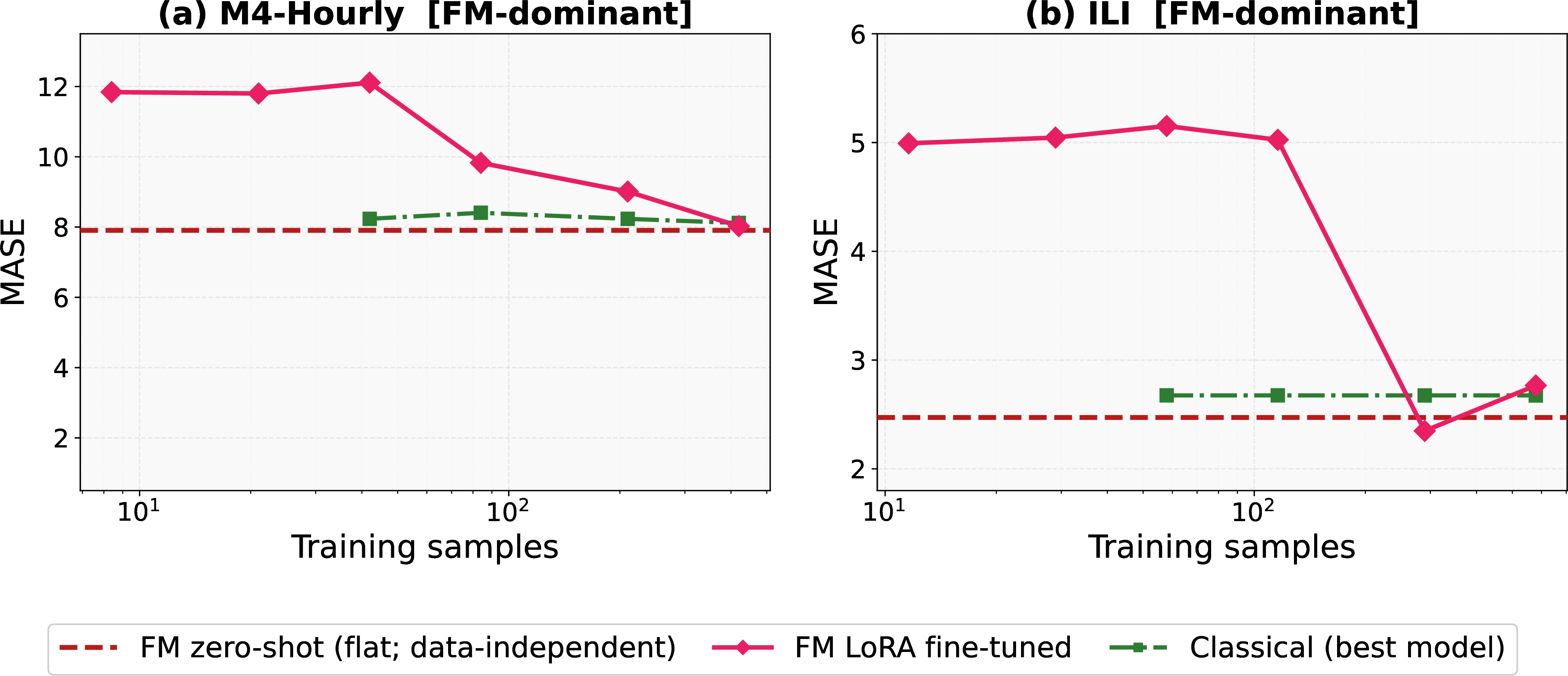
Finding 2: LoRA fine-tuning is selective. LoRA improves over zero-shot on 17 of 30 datasets at full training data, but gains are uneven. On FM-dominant datasets, fine-tuning does not help (M4-Hourly: best ZS Lag-Llama 7.906, best LoRA Chr-Bolt 8.025—LoRA 1.5% worse than zero-shot). On short series, fine-tuning further degrades performance (ILI, 966 total samples: Chronos-Bolt-S ZS 2.472, LoRA 2.766). The common assumption that fine-tuning generally improves over zero-shot does not hold unconditionally here.
Finding 3: Full fine-tuning carries data-regime-dependent risk. When sufficient data is available, full fine-tuning often matches or beats LoRA (22 of 30 datasets) and zero-shot (21 of 30 datasets) at full training data. However, at low training fractions (\(\leq\)5%), individual model–dataset combinations can fail catastrophically: Moirai-S reaches MASE \(=\) 23.6 on Solar-10min and Chronos-Bolt-S reaches 14.6 on M4-Daily, compared to zero-shot baselines of 0.92 and 2.10 respectively (109 cases with MASE \(>\) 10 across both model families). LoRA is more robust in the low-data regime (mean per-run seed std 0.095 vs. for full fine-tuning at fractions \(\leq\)5%) and is the safer default when training data is limited.
Finding 4: No single FM dominates across all datasets. Chronos-Bolt-S is best zero-shot on ILI; Moirai-L on Exchange; Chronos-Bolt-B on KDD-Cup-Hourly, Tourism-Monthly, and Wind-Farms. Moirai variants dominate FM-dominant datasets with low seasonal strength (ETTh1: \(S=0.28\), ETTm1: \(S=0.30\)) and fast ACF decay (Electricity: \(\tau_{\text{acf}}=3\)). Lag-Llama achieves best zero-shot on M4-Hourly, NN5-Daily, Pedestrian, Rideshare, Sunspot, and USBirths. Model selection is dataset-dependent even within the FM class.
Finding 5: XGBoost remains highly competitive among classical methods. Despite not leveraging pretraining, XGBoost achieves best classical performance on 14 of 30 datasets at full training data. On the 15 FM-dominant datasets, XGBoost is competitive but does not exceed the FM zero-shot baseline, which defines those datasets as FM-dominant by construction.
4.3 Determinants of Break-Even (RQ2)↩︎
| Dataset | \(n_{\text{train}}\) | \(\tau_{\text{acf}}\) | \(H\) | \(\sigma_r\) | \(S\) | \(\Phi\) | Pattern |
|---|---|---|---|---|---|---|---|
| Dominick | 54 | 2 | 0.77 | 0.94 | 0.00 | 0.76 | FM-dom. |
| ETTh1 | 10,452 | 200 | 0.94 | 0.12 | 0.28 | 0.27 | FM-dom. |
| ETTm1 | 41,808 | 200 | 1.00 | 0.06 | 0.30 | 0.23 | FM-dom. |
| Electricity | 15,782 | 3 | 0.69 | 0.54 | 0.63 | 0.56 | FM-dom. |
| Exchange | 4,552 | 200 | 1.00 | 0.05 | 0.00 | 0.18 | FM-dom. |
| ILI | 579 | 68 | 0.97 | 0.23 | 0.92 | 0.33 | FM-dom. |
| KDD-Cup-Hourly | 6,538 | 29 | 0.97 | 0.17 | 0.03 | 0.56 | FM-dom. |
| NN5-Daily | 474 | 1 | 0.55 | 1.11 | 0.88 | 0.52 | FM-dom. |
| Pedestrian | 13,355 | 4 | 0.65 | 0.41 | 0.94 | 0.27 | FM-dom. |
| Rideshare | 324 | 44 | 0.98 | 0.18 | 0.03 | 0.31 | FM-dom. |
| Sunspot | 44,354 | 200 | 0.87 | 0.35 | 0.14 | 0.49 | FM-dom. |
| Tourism-Monthly | 145 | 17 | 0.88 | 0.38 | 0.95 | 0.37 | FM-dom. |
| USBirths | 4,383 | 2 | 0.67 | 0.85 | 0.84 | 0.37 | FM-dom. |
| Wind-Farms | 316,224 | 200 | 1.00 | 0.03 | 0.02 | 0.26 | FM-dom. |
| M4-Hourly | 420 | 5 | 0.65 | 0.27 | 0.99 | 0.33 | FM-dom. |
| AusElectricity | 138,441 | 8 | 0.90 | 0.18 | 0.93 | 0.28 | Early |
| ETTh2 | 10,452 | 200 | 0.86 | 0.11 | 0.63 | 0.21 | Early |
| FRED-MD | 436 | 81 | 0.99 | 0.11 | 0.04 | 0.27 | Early |
| Saugeen | 14,244 | 10 | 0.93 | 0.36 | 0.41 | 0.63 | Early |
| Solar-10min | 31,536 | 21 | 0.98 | 0.06 | 0.91 | 0.17 | Early |
| Traffic | 10,526 | 2 | 0.66 | 0.74 | 0.63 | 0.61 | Early |
| Weather | 31,617 | 200 | 1.00 | 0.04 | 0.75 | 0.31 | Mid |
| COVID-Deaths | 127 | 22 | 1.00 | 0.03 | 0.00 | 0.35 | Late |
| ETTm2 | 41,808 | 200 | 1.00 | 0.04 | 0.63 | 0.18 | Late |
| Hospital | 50 | 1 | 0.73 | 1.57 | 0.58 | 0.75 | Late |
| M3-Monthly | 49 | 1 | 0.83 | 1.01 | 0.72 | 0.72 | Late |
| M3-Quarterly | 26 | 5 | 1.00 | 0.19 | 0.55 | 0.51 | Late |
| M4-Daily | 227 | 19 | 0.95 | 0.18 | 0.11 | 0.36 | Late |
| M4-Monthly-Monash | 57 | 15 | 0.94 | 0.45 | 0.37 | 0.47 | Late |
| M4-Weekly | 227 | 6 | 0.91 | 0.42 | 0.85 | 0.45 | Late |
3pt
\(n_{\text{train}}\) = training samples (60% split). \(\tau_{\text{acf}}\) capped at 200; \(H\) via R/S analysis (shown for reference — both features
saturate for long-memory series). The classifier in Section [sec:sec:rq3] uses unsaturated replacements: \(\overline{|\rho|}_{50}\) (mean
\(|\rho(k)|\), lags 1–50) and DFA-Hurst. \(\sigma_r\) = noise ratio. \(S\) = seasonal strength. \(\Phi\) = spectral entropy.
FM-dom. = FM-dominant.
Table 4 reveals two immediately notable observations. First, \(\tau_{\text{acf}}\) saturates at 200 for several datasets, and \(H\) (R/S Hurst) saturates near 1.0 for many long-memory series—indicating that scalar summaries cannot distinguish degrees of long-range dependence. Second, the most discriminative features turn out to be \(n_{\text{train}}\), \(S\), \(\sigma_r\), and \(\tau_{\text{acf}}\) (when not saturated), each capturing a distinct mechanism.
Pattern explanation.1
FM-dominant datasets (15) include a diverse mix: low seasonal strength (\(S < 0.35\): ETTh1, ETTm1, Exchange, KDD-Cup-Hourly, Wind-Farms), fast ACF decay with high seasonality (Electricity, Pedestrian, NN5-Daily, USBirths), short series (ILI, M4-Hourly, Rideshare, Tourism-Monthly, Dominick), and long periodic series (Sunspot). Exchange and Wind-Farms are FM-dominant under fixed-denominator MASE: predictions were identical at all fractions, and an unfixed denominator would inflate MASE at low fractions, masking FM dominance. M4-Hourly (\(n=420\), \(S=0.99\)) is FM-dominant because Lag-Llama zero-shot (MASE 7.906) outperforms XGBoost at every fraction; including Lag-Llama as a candidate FM is decisive here. Dominick (\(n=54\)) is FM-dominant due to data scarcity eliminating most classical fractions.
Early break-even (6 datasets) is more coherent than the original taxonomy: it is driven by large datasets with sufficient classical training data (AusElectricity \(n=138{,}441\); ETTh2 \(n=10{,}452\); Saugeen \(n=14{,}244\); Solar-10min \(n=31{,}536\); Traffic \(n=10{,}526\)) or, for FRED-MD, a combination of near-zero seasonality and short series where any small sample is enough for classical to adapt. High innovation noise (Traffic \(\sigma_r=0.74\)) also contributes by erasing the FM advantage quickly.
Late break-even datasets are predominantly short (\(n_{\text{train}} < 500\) for 7 of 8), where classical methods require most available data to accumulate sufficient signal. ETTm2 (\(n=41{,}808\)) is the sole long-series exception: classical only beats FM zero-shot at 20% of its large training corpus (\(n^*=8{,}361\)), making it a structural-Late rather than a data-starvation-Late case.
Mid break-even (1 dataset, Weather) has enough data that classical catches up at 10% (\(n^*=3{,}161\)). With only one dataset, the Mid category cannot be generalized; practitioners should treat Mid and Late as a single “substantial-data-required” regime.
Interpretation: The ETTh1/ETTh2 contrast remains instructive. Both are hourly energy datasets of identical length (17,420 samples), yet ETTh1 (\(S=0.28\)) is FM-dominant while ETTh2 (\(S=0.63\)) shows early break-even at \(n^*=209\) (2%). Similarly, ETTm1 (\(S=0.30\), FM-dominant) and ETTm2 (\(S=0.63\), Late) differ primarily in seasonal strength. These pairwise contrasts confirm that subtle differences in seasonal structure—not frequency or length—drive the break-even regime, and that break-even cannot be inferred from metadata alone.
4.4 Feature-Based Hypotheses for Break-Even Behavior (RQ3)↩︎
With 30 datasets, we fit a random forest classifier (500 trees, max depth 4) with LOO cross-validation: four-class accuracy is 53.3% (above the 50% majority-class baseline, FM-dominant accounting for 15/30) and three-class accuracy is 60.0% (above the 50% majority-class baseline; three-class merges Early\(+\)Mid into one class, giving FM-dom: 15, Early\(+\)Mid: 7, Late: 8). Both classifiers provide marginal above-chance signal at this benchmark scale. We therefore retain an exploratory framing, treating the LOO results as evidence of partial predictability rather than a validated classification tool.
What the features reveal. The classical Hurst exponent estimated via rescaled range (R/S) analysis saturates near 1.0 for many long-memory series, providing limited discriminative signal; we therefore use detrended fluctuation analysis (DFA) which does not saturate. Similarly, \(\tau_{\text{acf}}\) (lag where \(|\rho| < 0.5\)) saturates at 200 for many datasets; we replace it with \(\overline{|\rho|}_{50}\), the mean \(|\rho(k)|\) over lags 1–50, which is continuous and non-saturating. This unsaturated ACF feature retains a significant negative correlation with the Late pattern (\(r = -0.382\), \(p = 0.037\)). Crucially, it is not a necessary condition for Late: ETTm2 (Late, \(\overline{|\rho|}_{50} = 0.90\)) is a direct counterexample showing that high mean autocorrelation does not preclude Late break-even. The features that vary most meaningfully across our 30 datasets are \(n_{\text{train}}\), \(S\), \(\sigma_r\), and \(\overline{|\rho|}_{50}\). Notably, each appears to capture a qualitatively distinct mechanism.
Hypothesis 1: Data starvation drives late break-even. On short datasets, FM zero-shot wins not because pretrained representations are superior, but because classical methods lack enough samples to fit a reliable model. The FM advantage is passive: it disappears as soon as classical methods accumulate sufficient data. All Late and Mid datasets except ETTm2 (\(n=41{,}808\)) and Weather (\(n=31{,}617\)) have \(n_{\text{train}} < 700\). We therefore hypothesize that any sufficiently short series will exhibit late or mid break-even regardless of its temporal structure, with \(n_{\text{train}} \lesssim 700\) as a rough threshold (not a validated boundary)—chosen to include ILI (\(n=579\)), the largest short dataset in our benchmark, with a clear gap to the next cluster (\(n \geq 4{,}383\)). Fine-tuning is counterproductive in this regime: LoRA on ILI—an FM-dominant short dataset—degraded performance from MASE 2.472 to 2.766 (best LoRA across models), consistent with overfitting on an already limited sample.
Hypothesis 2: High innovation variance causes early break-even. FM pretraining captures general structure—seasonality, trends, smooth dynamics—but cannot anticipate the task-specific random behaviour of a particular dataset. When a series is dominated by large unpredictable innovations, pretrained representations carry no transferable advantage. Classical methods, by contrast, immediately learn local lag relationships and noise patterns from even a small task-specific sample. We hypothesize that innovation-dominated series therefore exhibit early break-even regardless of their length. Traffic (\(\sigma_r=0.74\), among the highest for long series in our benchmark) exhibits early break-even at just 2% of data, consistent with this mechanism. Note that short datasets such as Hospital (\(\sigma_r=1.57\)) have higher raw noise but show late break-even: data starvation (H1) dominates there, masking any innovation effect.
Hypothesis 3: Structural regime determines FM dominance for long series. For long series (\(n_{\text{train}} > 4000\)), data starvation (H1) is no longer the explanation—classical methods have ample data to fit. The determining factor instead becomes whether the dataset’s structure matches what FM pretraining can transfer. We observe two empirical sub-patterns among long series.
Sub-pattern A: Very low seasonal strength favours FM dominance. When \(S < 0.35\) (ETTh1, ETTm1), classical seasonal methods lose their primary anchor. FM representations appear to capture subtle long-range structure that classical methods miss even at full training data, resulting in FM dominance. Long series with moderate seasonality show later break-even: ETTh2 (\(S=0.63\)) is Early (\(n^*=209\), 2% of data) while ETTm2 (\(S=0.63\)) is Late (\(n^*=8{,}361\), 20% of 41,808). Both contrast sharply with their FM-dominant counterparts ETTh1/ETTm1, confirming that seasonal strength—not length—is the key determinant among long ETT series.
Sub-pattern B: Fast ACF decay combined with moderate-to-high seasonality favours FM dominance. Electricity (\(\tau=3\), \(S=0.63\)), Pedestrian (\(\tau=4\), \(S=0.94\)), and USBirths (\(\tau=2\), \(S=0.84\)) are all FM-dominant. We tentatively attribute this to short memory providing a stable seasonal signal that FM pretraining transfers well, while the fast decay means classical methods cannot exploit long-range dependence to compensate. However, fast ACF decay alone is not sufficient: AusElectricity (\(\tau=8\), \(S=0.93\)) and Saugeen (\(\tau=10\), \(S=0.41\)) satisfy the same condition yet show early break-even, suggesting the boundary depends on additional factors the current feature set does not capture.
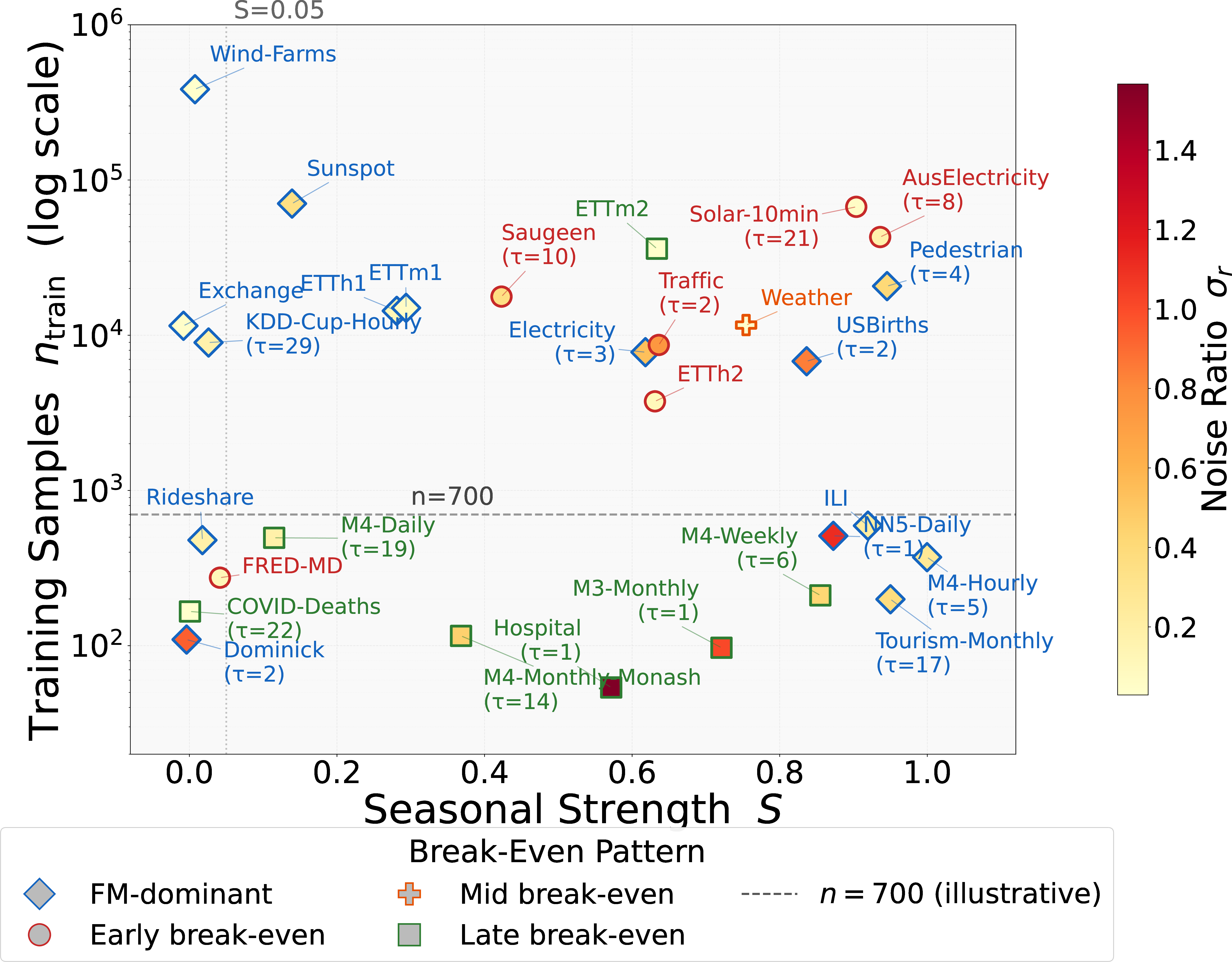
Figure 2 plots \(n_{\text{train}}\) versus seasonal strength \(S\) for all 30 datasets, with marker shape encoding break-even pattern and colour encoding noise ratio \(\sigma_r\). Late break-even datasets (triangles) cluster at low \(n\) regardless of seasonality, consistent with data starvation (H1) as the dominant driver. FM-dominant and Early break-even datasets overlap substantially at high \(n\) and moderate–high \(S\) (e.g., AusElectricity Early \(S=0.93\) vs.Pedestrian FM-dominant \(S=0.94\)): noise ratio provides additional separation in this region but does not cleanly resolve the boundary, motivating the pilot-experiment fallback in the decision framework.
5 Analysis and Discussion↩︎
5.1 The Role of Fine-Tuning↩︎
Figure 3 compares zero-shot and LoRA fine-tuned performance on two FM-dominant datasets. LoRA does not reliably improve over zero-shot and can actively degrade performance, particularly on short series where it risks overfitting a limited sample. The determining factor is whether the series structure aligns with pretrained representations: when FM zero-shot already captures the relevant patterns, fine-tuning adds noise rather than signal.
5.2 Practical Decision Support (RQ3)↩︎
Automated classification is marginally above chance (60.0% three-class LOO vs.% majority-class baseline; 53.3% four-class LOO vs.% majority-class baseline). One individual signal nonetheless provides robust practical guidance:
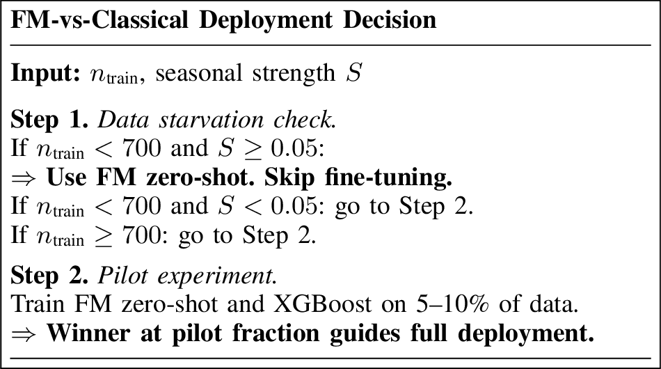
The data starvation rule is robust. If \(n_{\text{train}} < 700\) and \(S \geq 0.05\), use FM zero-shot: classical methods cannot accumulate sufficient signal from a small fraction of an already short dataset. Avoid LoRA fine-tuning in this regime. This resolves 10 of 30 benchmark datasets (4 FM-dominant, 6 Late) without any model training. Exception: if \(n_{\text{train}} < 700\) and \(S < 0.05\), the FM advantage is not guaranteed (FRED-MD: \(n^*=21\)); run a pilot experiment first.
The ACF feature cannot serve as a decision rule. ETTm2 (Late, \(\overline{|\rho|}_{50}=0.90\)) shows that no low-ACF threshold reliably identifies Late break-even. The feature retains a significant correlation with Late (\(r=-0.382\), \(p=0.037\)) but is insufficient for reliable classification. For all cases not resolved by the data starvation rule, a pilot experiment is required.
Practical implication. Figure 4 formalises these signals as a two-step deployment procedure. Step 1 resolves the FM-vs-classical decision without any model training on 10 of 30 datasets; Step 2 (pilot experiment at 5–10% of data) covers the remaining 20 cases where features alone are insufficient.
5.3 Limitations↩︎
Dataset scale: With 30 datasets, LOO cross-validation yields 60.0% three-class accuracy and 53.3% four-class accuracy (both above the 50% majority-class baseline)—insufficient for reliable automated selection. The taxonomy (FM-dominant: 15/30) raises the majority-class baseline, making the classification task harder. Validating generalizable decision boundaries requires a benchmark of 50+ datasets spanning more diverse domains. Features R/S Hurst and \(\tau_{\text{acf}}\) were replaced by DFA Hurst and \(\overline{|\rho|}_{50}\) to eliminate ceiling saturation; residual discriminative limitations persist at this benchmark scale.
Univariate evaluation: All experiments target a single output series (OT column) from each dataset. Multivariate FM capabilities—a key advantage of Moirai—are not evaluated.
Foundation model evolution: Foundation models improve rapidly. Our results reflect models available as of early 2026; newer models may shift break-even dynamics.
Full fine-tuning instability: Full fine-tuning is unstable at low fractions (\(\leq\)5%), with 109 catastrophic failures (MASE \(>\) 10) and worst-case MASE exceeding 23 (Moirai-S on Solar-10min). Results are omitted from main tables; LoRA is the recommended default.
6 Conclusion↩︎
We introduced break-even analysis as a framework for evaluating foundation models against classical alternatives. Our systematic experiments across 30 datasets (10,800 configurations: 30 datasets \(\times\) 6 fractions \(\times\) 20 model-settings \(\times\) 3 seeds) reveal that the foundation model advantage is not universal but depends critically on dataset properties and available data volume.
Foundation models outperform classical methods at every evaluated training fraction on 15 of 30 datasets—FM-dominant is the plurality category, and zero-shot FM is the recommended choice on these datasets regardless of data volume. On 6 datasets, classical methods surpass zero-shot FMs with as little as 2% of training data (21–2,768 samples); for practitioners with even modest historical data in these regimes, XGBoost is preferable. These two extremes leave 9 datasets in the mid-to-late break-even range, where the FM advantage erodes only after substantial classical training data accumulates.
LoRA fine-tuning is beneficial only on specific dataset types—particularly those with clear periodicity and sufficient length—and actively degrades performance on short series. On ILI, LoRA raises MASE from 2.472 to 2.766 despite classical never beating FM zero-shot at any fraction, a case where fine-tuning adds instability to an already FM-dominant regime. XGBoost remains a strong classical competitor, achieving best classical performance on 14 of 30 datasets at full data, confirming that FM adoption must be justified against well-tuned gradient boosting baselines.
Four dataset features—series length (\(n\)), seasonal strength (\(S\)), noise ratio (\(\sigma_r\)), and mean autocorrelation (\(\overline{|\rho|}_{50}\))—co-vary with break-even patterns and motivate mechanistic hypotheses. One rule is empirically robust: \(n_{\text{train}} < 700\) with \(S \geq 0.05\) reliably identifies the FM zero-shot regime, resolving 10 of 30 deployment decisions without any model training. Beyond this rule, no single feature threshold suffices, and a pilot experiment remains necessary. Dataset-level assessment—particularly series length and seasonality strength—should guide the FM-versus-classical decision; our break-even analysis provides a principled framework for making that decision before committing to full infrastructure.
We release our benchmark, analysis code, and feature extraction tools at https://github.com/nicolaisi/fm-breakeven.