On the Complexity of Entrywise Power Matrix Factorization
July 06, 2026
Abstract
Given a nonnegative matrix \(X\), a factorization rank \(r\) and a real parameter \(p\), entrywise power matrix factorization (EPMF) looks for a low-rank matrix \(X_r\) such that \(X = |X_r|^{\circ p}\) (exact case) or \(X \approx |X_r|^{\circ p}\) (approximate case), where \((\cdot)^{\circ p}\) denotes the component-wise exponent. EPMF includes the modulus model (\(p=1\)) and component-wise square factorization (\(p=2\)) as special cases, the latter being closely related to the square root rank. We analyze the computational complexity of the exact decision problem and the Frobenius-norm approximation problem, and establish a complete complexity landscape. In the exact case, we show that EPMF is equivalent to the combinatorial problem of flipping the signs of the entries of a given matrix \(X\) to obtain a rank-\(r\) matrix, which we refer to as the signing problem. We first show that the signing problem, and hence exact EPMF, is strongly NP-hard, improving a weak NP-hardness result for the square-root-rank of Fawzi et al. (Math.Prog., 2015). We then show that the signing problem can be solved in polynomial-time when \(r\) is fixed. Moreover, when the rank \(r\) is part of the input, we show that for generic matrices the algorithm is fixed-parameter tractable (FPT) in the parameter \(r\); in fact, the running time is linear in the input size \(X\). In the approximate case using the Frobenius norm as an error measure, we show that EPMF is NP-hard, already when \(r=2\), the smallest nontrivial case.
Keywords: nonlinear matrix decompositions, entrywise power matrix factorization, signless rank, fixed-parameter tractable, strong NP-hardness.
1 Introduction↩︎
Low-rank matrix approximation is a central tool in numerical linear algebra, data analysis, machine learning, and signal processing. Given a data matrix \(X\in\mathbb{R}^{m\times n}\) and an integer \(r \leq \min(m,n)\), the classical problem is to approximate \(X\) by a matrix of rank at most \(r\), or, equivalently, to find factors \(W\in\mathbb{R}^{m\times r}\) and \(H\in\mathbb{R}^{r\times n}\) such that \(X\approx WH\). This is equivalent to linear dimensionality reduction: each column of \(X\) is approximated by a linear combination of the columns of \(W\). The best known example is the truncated singular value decomposition (SVD), which gives an optimal rank-\(r\) approximation in the Frobenius norm, and any unitary invariant norm, by the Eckart–Young theorem [1]–[3]. Many variants, including robust PCA, sparse PCA, weighted low-rank approximation, and matrix completion, modify the loss function or impose additional constraints in order to reflect the structure of the data; see, e.g., [4] and the references therein. The computational complexity of such models has been studied in depth. Computing the (truncated) SVD is a classical problem in numerical linear algebra, and can be done in polynomial time in \(m, n, r\) and \(\log(1/\varepsilon)\), where \(\varepsilon\) is the desired precision; see, e.g., [2], [3]. The SVD can be used to compute the best rank-\(r\) approximation in any unitary invariant norm, including the matrix \(\ell_2\) norm and the Frobenius norm. However, as soon as different norms are used, finding the best rank-\(r\) approximation becomes NP-hard, already when \(r=1\); this is true for the component-wise \(\ell_1\) [5] and \(\ell_\infty\) norms [6], and weighted norms or when data is missing [7]. Moreover, by writing \(X_r = WH\), where \(W\) has \(r\) columns and \(H\) has \(r\) rows, it is often useful in practice to add constraints on the factors, \(W\) and \(H\), typically to improve the interpretability of the decomposition. For example, sparsity leads to sparse PCA and variants, and imposing a given sparsity pattern to the factors leads to an NP-hard problem [8]. Another famous example is nonnegativity constraints leading to nonnegative matrix factorization (NMF) which is also NP-hard [9], but can be solved in polynomial time in the exact case (that is, find, if possible, \(W \geq 0\), \(H \geq 0\) such that \(X = WH\)) when \(r\) is treated as a constant, with a complexity of \((mn)^{\mathcal{O}(r^2)}\) operations [10]. Analogous results were obtained for the positive semidefinite factorization [11], [12]. These results study worst-case complexity, but luckily there is a plethora of low-rank models that are tractable under reasonable assumptions. Two of the most widely known approaches to obtain such results are based on minimizing the nuclear norm as a proxy for the rank [13], or on proving that the the optimization landscape does not have spurious local minima, that is, all local minima are global [14], [15]. This has been done for missing data [16], [17], robust variants that rely on other metrics than the Frobenius norm [18], [19], NMF under the so-called separability assumption [10], and binary matrix decompositions [20], [21], to cite a few. It is out of the scope of this paper to review this literature.
Despite their success, linear low-rank models have limited expressive power. Many data sets exhibit nonlinear structures that they cannot capture. This limitation has motivated the recent introduction of nonlinear matrix decompositions (NMDs) [22], in which one approximates a matrix by applying a nonlinear function entrywise to a low-rank matrix \(X_r\): \[X\approx f(X_r).\] Different choices of \(f\) lead to different models and allow for various structural assumptions about the data. A prominent example is the ReLU model, \(X \approx \max(0,X_r)\), introduced by Saul for sparse nonnegative data [22]. Since then, several algorithmic approaches have been proposed for this model, including coordinate-descent schemes [23], accelerated alternating partial Bregman proximal gradient method [24], and extrapolated block coordinate methods [25]. Another example is the component-wise square factorization (CSF), \(X\approx (WH)^{\circ 2}\). CSF is closely related to the square-root rank of nonnegative matrices, a quantity that appears in the compact representation of convex polytopes [26], [27]. CSF is also related to the fixed-rank signing problem: given a matrix \(M \in \mathbb{R}^{m \times n}\) and an integer \(r \leq \min(m,n)\), decide whether there exists a sign matrix \(S \in \{\pm 1\}^{m \times n}\) such that \(\rank(S \circ M) \leq r\). Fixed-rank signing is connected to the signless rank of a matrix, denoted by \(\rank_{\pm}(A)\), which is defined as the minimum rank of \(S \circ A\) over all sign matrices \(S \in \{\pm 1\}^{m \times n}\) [28]. We will study this problem in Sections 2.2 and 3. A natural generalization of the signless rank for complex matrices is referred to as the phaseless rank of a matrix [28] which is connected to the notion of equimodular classes of matrices [29]. CSF has also been used to obtain compact representations of nonnegative data and probabilistic circuits [30], and recent work has developed coordinate-descent algorithms for the associated least-squares problem [31].
CSF is also closely related to the Hadamard decomposition, defined as \(X \approx X_1 \circ X_2\), where \(X_i\) are low-rank matrices and \(\circ\) is the component-wise Hadamard product, that has been successfully used for example to compress or adapt neural networks [32], [33]; see [34] and the references therein for more details. The modulus model, \(X\approx |WH|\), provides another unconstrained factorization model for nonnegative data [35]. Other nonlinearities, such as min-max and sigmoid functions, have also been considered in applications with bounded or binary observations [35], [36].
1.0.0.1 Outline and contribution of the paper
The computational complexity of (linear) low-rank matrix approximations has been extensively studied; see the first paragraph of Section 1. However, for non-linear models, computational complexity has not been explored yet. In this paper, we focus on entrywise power matrix factorization (EPMF), which unifies the modulus and component-wise square cases. For a fixed \(p\), it considers the decomposition \(X \approx |X_r|^{\circ p}\), where \(X_r\) is a rank-\(r\) matrix, and the absolute value and the power are applied entrywise. We consider two variants: Given a nonnegative matrix \(X\), a factorization rank \(r\) and a parameter \(p\in \mathbb{R}\),
ExactEPMF: compute, if possible, a rank-\(r\) matrix \(X_r\) such that \(X = |X_r|^{\circ p}\).
FroEPMF: find a rank-\(r\) matrix \(X_r\) that minimizes \(\left\|X - |X_r|^{\circ p}\right\|_F^2\).
Our positive result concerns the exact fixed-rank regime. After taking the entrywise \(p\)th root of \(X\), the problem ExactEPMF becomes a signing problem: given a nonnegative matrix \(M\), decide whether one can choose the signs of its entries so that the resulting matrix has rank at most \(r\). We show that, for fixed \(r\), this problem can be solved in polynomial time. As for exact NMF, the problem is polynomial-time solvable for fixed rank, although the exponent of the polynomial in the dimension of the input depends on \(r\). The algorithm enumerates all possible sign patterns of non-singular basis \(r\)-by-\(r\) blocks, but it avoids a global enumeration of the signs by using the linear dependencies. Moreover, even when \(r\) is given as a part of the input, if the input matrix is generic, we show that the algorithm is fixed-parameter tractable (FPT), that is, it requires \(f(r).\text{poly}(m,n)\) number of operations where \(f\) is a computable function.
Our hardness results show that this favorable behavior is specific to exact fixed-rank feasibility or generic settings. When the rank is part of the input, we show that ExactEPMF is strongly NP-hard, by a reduction from monotone not-all-equal 3-SAT, generalizing and improving a weak NP-hardness result for the square-root-rank case of Fawzi et al. [27]. Moreover, we show that the least-squares formulation, FroEPMF, is NP-hard, already for \(r=2\), via a reduction from the decision version of the cut-norm problem.
The paper is organized as follows. Section 2 proves strong NP-hardness of ExactEPMF when the rank \(r\) is part of the input. When the rank \(r\) is not part of the input, meaning it is treated as a constant, we provide in Section 3 a polynomial-time algorithm for ExactEPMF. Moreover, in Section 3.2.3 we show that this algorithm is fixed-parameter tractable (FPT) for generic input matrices even when \(r\) is a part of the input. Section 4 proves NP-hardness of FroEPMF, already when \(r=2\), the first non-trivial case. Section 5 draws the conclusions and the appendix includes some technical lemmas. Table 1 summarizes our results.

1.0.0.2 Notation
For the first \(n\) natural numbers, we use the standard notation \([n]=\{1,\dots,n\}\). The vectors \(e_1,\dots,e_n\) denote the canonical basis of \(\mathbb{R}^{n\times n}\). For a matrix \(A\), we use a Matlab-like notation: we denote its \(i\)th row by \(A(i,:)\), its \(j\)th column by \(A(:,j)\) and its \((i,j)\) entry by \(A(i,j)\), sometimes also indicated with the lowercase associated letter \(a_{ij}\). We use \(\circ\) for the entrywise multiplication, both for matrices and vectors, but also for the \(p\)th entrywise power of a matrix \(A\), which is denoted by \(A^{\circ p}\). The transpose of \(A\) is \(A^\top\). For any vector \(v\), \(\mathop{\mathrm{diag}}(v)\) is the diagonal matrix whose diagonal is \(v\), and \(\|v\|=\sqrt{\langle v,v\rangle}\) is the \(\ell_2\)-norm of \(v\). The all-zeros matrix and the all-ones matrix of size \(m\times n\) are denoted, respectively, by \(\mathbf{0}_{m\times n}\) and \(\mathbf{1}_{m\times n}\), and in case of the vectors we write \(\mathbf{0}_n\) and \(\mathbf{1}_n\). The \(n\times n\) identity matrix is \(I_n\).
2 NP-hardness of ExactEPMF↩︎
We first consider ExactEPMF when the rank is part of the input. We first generalize the result of Fawzi et al. [27], which proves the weak NP-hardness of computing the square-root rank, that is, ExactEPMF for \(p=2\), using a reduction from PARTITION which is weakly NP-hard [37]; see Section 2.1. We then prove strong NP-hardness in Section 2.2.
2.1 Weak NP-hardness↩︎
The reduction below is a direct adaptation of the construction of Fawzi et al. [27] from PARTITION, which we provide here for completeness. Let us formally define the decision versions of both problems.
Let \(S\) be an instance of PARTITION. We construct an instance \((X,r)\) of ExactEPMF in polynomial time as follows. Set \(m = n = N+1\) and \(r=N\). Using \(s=(s_1,\ldots,s_N)^\top\), set \[X= \begin{pmatrix} I_N & s^{\circ p}\\ \mathbf{1}_N^\top &
0 \end{pmatrix} \in\mathbb{R}_{\ge0}^{(N+1)\times(N+1)}.\]
The construction is polynomial in the size of the input since \(p\) is fixed. Intuitively, the reduction relies only on the freedom of choosing signs of prescribed entrywise \(p\)th roots.
Theorem 1. The instance \((X,r)\) is a yes-instance of ExactEPMF if and only if \(S\) is a yes-instance of PARTITION. Hence, ExactEPMF is weakly NP-hard when \(r\) is part of the input.
Proof. If part. Suppose that \(S\) is a yes-instance of PARTITION. Then there exist signs \(\sigma_i\in\{\pm1\}\) such that \(\sum_{i=1}^N \sigma_i s_i=0\). Define \[Y=\begin{pmatrix} I_N & s\\ \sigma^\top & 0 \end{pmatrix}.\] Then \(|Y|^{\circ p}=X\). The last row of \(Y\) is the linear combination of the first \(N\) rows with coefficients \(\sigma_1,\ldots,\sigma_N\) since \(\sum_{i=1}^N \sigma_i s_i=0\). Thus \(\rank(Y)\leq N=r\). Therefore \(X=|WH|^{\circ p}\) for some \(W\in\mathbb{R}^{(N+1)\times N}\), \(H\in\mathbb{R}^{N\times(N+1)}\), so the ExactEPMF instance is a yes-instance.
2.1.0.1 Only if part.
Suppose that the ExactEPMF instance is a yes-instance. Then there exists a matrix \(Y\) such that \(|Y|^{\circ p}=X\), \(\rank(Y)\leq N\). Since the upper-left block of \(X\) is \(I_N\), the corresponding block of \(Y\)is a signed identity matrix, hence is invertible. Therefore \(\operatorname{rank}(Y)\geq N,\) and so \(\operatorname{rank}(Y)=N\). The first \(N\) columns of \(Y\) are linearly independent, and the last column must lie in their span, that is, \(Y(:,N+1)=\sum_{i=1}^N \alpha_i Y(:,i)\) for some \(\alpha\)’s. The first \(N\) entries of this relation indicate that \(\alpha_i=\pm s_i\) while the last one gives \(\sum_{i=1}^N \sigma_i s_i=0\) for some signs \(\sigma_i\in\{\pm1\}\). Hence, the PARTITION instance is a yes-instance. ◻
2.2 Strong NP-hardness↩︎
To prove strong NP-hardness of ExactEPMF, we rely on the monotone Not-All-Equal 3-Satisfiability problem (NAE-3SAT).
For Boolean variables, \(x_1,\dots,x_n\in\{0,1\}\), \(\text{NAE}(x_1,\dots,x_n)\) is satisfied by the assignment \(x\) if and only if there exists \(i \neq j \in [n]\) such that \(x_i\) is \(1\) and \(x_j\) is \(0\). We say that a map \(\phi: \{0,1\}^n \xrightarrow[]{} \{0,1\}\) is an instance of the Monotone NAE-3SAT problem if it can be written as \[\phi = \bigwedge_{l=1}^m \text{NAE}(x_{i_l}, x_{j_l}, x_{k_l})\] over Boolean variables \(x_1, \dots, x_n\). Monotone NAE-3SAT is known to be NP-complete, even under different restrictions [38], [39]. Here it is the decision versions the problem and the version of the ExactEPMF we want to compare with:
To prove strong NP-hardness of ExactIntegerEPMF, we rely on the following intermediate combinatorial problem.
Given a nonnegative matrix \(M\), fixed-rank signing requires to flip some signs of the entries of \(M\) in order to make it rank at most \(r\). This problem
is equivalent to ExactIntegerEPMF on instances of the form \(X=M^{\circ p}\), where \(p \in \mathbb{N}\) is fixed. Indeed, if \(S\circ M=WH\) with \(\rank(WH)\leq r\), then \[X=M^{\circ p}=|S\circ M|^{\circ p}=|WH|^{\circ p},\] so \((X,r)\) is a
yes-instance of ExactIntegerEPMF. Conversely, if \(X=M^{\circ p}=|WH|^{\circ p}\), then \(|WH|=M\), and hence \(WH=S\circ M\)
for the sign matrix \(S=\operatorname{sign}(WH)\), with \(\rank(S\circ M)\leq r\). Therefore, it suffices to prove strong NP-hardness of the fixed-rank signing problem for nonnegative
integer matrices. The corresponding hardness result for ExactIntegerEPMF then follows immediately by mapping \(M\) to \(M^{\circ p}\).
2.2.0.1 The reduction
For a Monotone NAE-3SAT instance \(\phi = \land_{l=1}^m \text{NAE}(x_{i_l}, x_{j_l}, x_{k_l})\) over \(n\) variables \(x_1, \dots, x_n\), we define the \(m \times n\) matrix \(H_{\phi}\) with the \(\ell\)th row corresponding to the \(\ell\)th \(\text{NAE}\) clause given by \((e_{i_\ell} + e_{j_\ell} + e_{k_\ell})^\top\). We then construct the following \((m+n+3) \times (n+4)\) matrix \[\label{eq:defninstanceAphi} M_\phi = \left( \begin{array}{cccc|c} 1 & 1 & 0 & 0 & \mathbf{0}_{1\times n}\\ 1 & 0 & 1 & 0 & \mathbf{0}_{1\times n}\\ 5 & 0 & 0 & 1 & \mathbf{0}_{1\times n}\\ \hline \mathbf{0}_{n\times 1} & \mathbf{1}_{n} & 2\mathbf{1}_{n} & \mathbf{0}_{n\times 1} & I_n\\ \hline \mathbf{0}_{m\times 1} & \mathbf{0}_{m\times 1} & \mathbf{0}_{m\times 1} & \mathbf{1}_{m} & H_\phi \end{array} \right).\tag{1}\] Note that for all sign patterns \(S \in \{\pm 1\}^{(m+n+3) \times (n+4)}\), \(\rank(S \circ M_\phi) \in \{n+3, n+4\}\). Indeed consider the sub-matrix with the last \(n+3\) columns and the first \(n+3\) rows: \[S(1:n+3,2:n+4)\circ \left(\begin{array}{c|c} I_3 & 0 \\ \hline * & I_n \end{array}\right),\] which has a non-zero determinant regardless of the sign flips, hence \(n+3 \leq \rank(S \circ M_\phi) \leq n+4\).
We can now prove the following result.
Theorem 2. The instance \(\phi\) is satisfiable if and only if there exists a sign pattern \(S\) such that \(\rank(S \circ M_{\phi}) = n+3\).
Proof.* If part** Any assignment \(x\) of \(\phi\) uniquely determines \[\tilde{z}(x)= \begin{pmatrix} 1 \\ 1 \\ 1 \\ 5 \\ z \\ \end{pmatrix}, \qquad S_\phi(x)= \left( \begin{array}{cccc|c} 1 & -1 & 1 & 1 & {\mathbf{1}}_n^\top \\ 1 & 1 & -1 & 1 & {\mathbf{1}}_n^\top \\ 1 & 1 & 1 & -1 & {\mathbf{1}}_n^\top \\ \hline {\mathbf{1}}_n & {\mathbf{1}}_n & -v & {\mathbf{1}}_n & \mathop{\mathrm{diag}}(v) \\ \hline {\mathbf{1}}_m & {\mathbf{1}}_m & {\mathbf{1}}_m & -{\mathbf{1}}_m & \Sigma \\ \end{array} \right),\] where \(z=z(x)=2x+{\mathbf{1}}_n\), \(v=v(x) = \mathbf{1}_n-2x \in \{\pm 1\}^n\) and \(\Sigma=\Sigma_\phi(x)\in \{\pm 1\}^{m\times n}\) is such that \[\Sigma(\ell,[i_\ell,j_\ell,k_\ell])=[f(x_{i_\ell},\sigma_{\ell}),f(x_{j_\ell},\sigma_{\ell}),f(x_{k_\ell},\sigma_{\ell})] \; \text{ for all \ell\in[m]},\] with \[f(y,\sigma)=y- (-1)^\sigma(1-y)\in\{\pm1\},\;\text{ where } y \in \{0,1\} \text{ and } \sigma_{\ell}=x_{i_\ell}+x_{j_\ell}+x_{k_\ell},\] and the other entries of \(\Sigma\) are equal to \(1\). Note that \(\sigma_\ell \in \{1,2\}\) for an instance to be satisfied. One can check that \(x\) satisfies \(\phi\) if and only if \(\tilde{z}=\tilde{z}(x)\) is in the kernel of \[M_\phi \circ S_\phi(x)= \left( \begin{array}{cccc|c} 1 & -1 & 0 & 0 & {\mathbf{0}}_n^\top \\ 1 & 0 & -1 & 0 & {\mathbf{0}}_n^\top \\ 5 & 0 & 0 & -1 & {\mathbf{0}}_n^\top \\ \hline {\mathbf{0}}_n & {\mathbf{1}}_n & -2v & {\mathbf{0}}_n & \mathop{\mathrm{diag}}(v) \\ \hline {\mathbf{0}}_m & {\mathbf{0}}_m & {\mathbf{0}}_m & -{\mathbf{1}}_m & \Sigma\circ H_\phi \\ \end{array} \right).\] Let us denote \[\label{eq:abc} \begin{pmatrix} a \\ b \\ c \\ \end{pmatrix}=(M_\phi\circ S_\phi)\tilde{z}, \qquad a\in \mathbb{R}^3, \;b\in \mathbb{R}^n, \;c\in \mathbb{R}^m.\tag{2}\] Let \(x\) be an assignment that satisfies \(\phi\). The vector \(a\) is zero by the choice of \(\tilde{z}\). For every entry of \(b\), \[b_i=1-2 v_i+v_i \tilde{z}_{i+4}=1-2(-2x_i+1)+(-2x_i+1)(2x_i+1)=1+4x_i-2-4x_i+1=0,\] where we used \(x_i^2=x_i\). Moreover, for every \(\ell\in[m]\), \[\begin{align} c_\ell & = -5+\sum_{h\in\{i,j,k\}}(2x_{h_\ell}+1)(x_{h_\ell}-(-1)^{\sigma_\ell}(1-x_{h_\ell}))\\ & = -5+\sum_{h\in\{i,j,k\}} 3x_{h_\ell}-(-1)^{\sigma_\ell}+(-1)^{\sigma_\ell} x_{h_\ell} =-5+3{\sigma_\ell} -3(-1)^{\sigma_\ell}+(-1)^{\sigma_\ell} {\sigma_\ell}, \end{align}\] which vanishes if and only if \(\sigma_\ell\in \{1,2\}\), that are exactly the values corresponding to an assignment \(x\) that satisfies \(\phi\).*
Only if part. Suppose that \(\rank(S\circ M_\phi)=n+3\) for some \(S\in\{\pm1\}^{(m+n+3)\times(n+4)}\). Let \(\tilde{z}\neq 0\) span the one-dimensional kernel of \(S\circ M_\phi\). We may assume w.l.o.g.that \(\tilde{z}\geq0\) since flipping the signs of the \(j\)th column of \(S\) and of the entry \(\tilde{z}_j\) leaves the equations \((S\circ M_\phi)\tilde{z}=0\) unchanged. Since \(\tilde{z}\geq0\), the three first equations forces the equality of the absolute values of its two terms. Thus \[\tilde{z}_1=\tilde{z}_2=\tilde{z}_3, \qquad \tilde{z}_4=5\tilde{z}_1.\] If \(\tilde{z}_1=0\), then \(\tilde{z}_2=\tilde{z}_3=\tilde{z}_4=0\), and the \(i\)th equation gives \(\tilde{z}_{4+i}=0\) for all \(i\), contradicting \(\tilde{z}\neq0\). Hence we may assume \(\tilde{z}_1=1\) by rescaling, and therefore \(\tilde{z}_2=\tilde{z}_3=1\), \(\tilde{z}_4=5\). The \((3+i)\)th row of \(S\circ M_\phi\) gives \[S(3+i,2)+2S(3+i,3)+S(3+i,4+i)\tilde{z}_{4+i}=0.\] It means that \(\tilde{z}_{4+i} = |S(3+i,2)+2S(3+i,3)|\in\{1,3\}\) since \(S(3+i,2)+2S(3+i,3)\in\{\pm1,\pm3\}\). We set \[x_i=\frac{\tilde{z}_{4+i}-1}{2}\in\{0,1\}.\] Finally the equations for the part \(c\) of equation 2 imply that \(x\) is an assignment that satisfies \(\phi\). In fact, for the \(\ell\)th clause in \(\phi\) of the form \(\mathrm{\small NAE}(x_{i_\ell},x_{j_\ell},x_{k_\ell})\), the corresponding \((n+3+\ell)\)th row of \(S \circ M_{\phi}\) has the form \(\pm 5 \pm \tilde{z}_{4+i_\ell} \pm \tilde{z}_{4+j_\ell} \pm \tilde{z}_{4+k_\ell}\). Since, \(\tilde{z}_{4+i} \in \{1,3\}\) for all \(i \in [n]\), if the three variables \(z_{4+i_\ell}, z_{4+j_\ell}, z_{4+jk_\ell}\) are equal to \(1\), the sum can be at most \(3\), so it cannot cancel out \(5\). Hence, all three \(x_{i_\ell},x_{j_\ell},x_{k_\ell}\) cannot be \(0\) together. If all these three entries of \(\tilde{z}\) are set to \(3\), which corresponds to the case when all \(x_{i_\ell},x_{j_\ell},x_{k_\ell}\) are equal to \(1\), the sum \(\pm \tilde{z}_{4+i_\ell} \pm \tilde{z}_{4+j_\ell} \pm \tilde{z}_{4+k_\ell} \in \{\pm 3, \pm 9\}\), and hence cannot cancel out \(5\). Thus we can conclude that \(x\) is an assignment that satisfies \(\phi\). ◻
Corollary 1. Exact Integer EPMF is strongly NP-hard when \(r\) is part of the input.
**Proof.* We give a polynomial-time many-one reduction from Monotone NAE-3SAT to Integer ExactEPMF. Let \[\phi=\bigwedge_{l=1}^{m}\operatorname{NAE}(x_{i_l},x_{j_l},x_{k_l})\] be a monotone NAE-3SAT instance over the variables \((x_1,\dots,x_n)\). Let \(M_\phi\in~\mathbb{Z}^{(m+n+3)\times(n+4)}\) be as in 1 , \(X_\phi:=M_\phi^{\circ p}\) and set \(r_\phi:=n+3\). Since \(p\) is fixed, this construction is computable in polynomial time in the size of \(\phi\) and hence \((X_\phi,r_\phi)\) is a valid instance of ExactEPMF. We show that \((X_\phi,r_\phi)\) is a yes-instance of ExactEPMF if and only if there exists \(S \in \{\pm 1\}^{m+n+3 \times n+4}\) such that \(\rank(S \circ M_\phi) \leq r_\phi\).*
If part. Suppose that \((X_\phi,r_\phi)\) is a yes-instance of ExactEPMF. Then there exist matrices \(W \in \mathbb{R}^{m + n + 3 \times r_\phi}\) and \(H \in \mathbb{R}^{r_\phi \times n+4}\) such that \(X_\phi = |WH|^{\circ p}\). Then \(M_\phi = X_\phi^{\circ \frac{1}{p}} = |WH|\) and hence, there exists a sign matrix \(S\) such that \(S \circ M_\phi = WH\). Hence \(\rank(S\circ M_\phi) \leq r_\phi\).
Only if part. Suppose there exists a sign matrix \(S\) such that \(\rank(S \circ M_\phi) \leq r_\phi\). Then \(S \circ M_{\phi} = WH\) for some matrices \(W \in \mathbb{R}^{m + n + 3 \times r_\phi}\) and \(H \in \mathbb{R}^{r_\phi \times n+4}\). Since \(M_\phi \geq 0\), taking entrywise absolute values on both sides, we get that \(M_\phi = |WH|\) and consequently, \(X_\phi = |WH|^{\circ p}\) which shows that \((X_\phi,r_\phi)\) is a yes-instance of ExactEPMF.
Using this and Theorem 2, we conclude that \(\phi\) is a satisfiable instance of Monotone NAE-3SAT if and only if \((X_\phi,r_\phi)\) is a yes-instance of ExactEPMF. ◻
3 Tractable algorithms for ExactEPMF↩︎
We now turn on positive results. We first show in Section 3.1 that the fixed-rank signing problem can be solved in polynomial time when \(r\) is fixed. In fact, we propose and implement an algorithm to do so (Algorithm 2). Then in Section 3.2, we propose two improvements of this algorithm which allow us to show that our algorithm is FPT in the rank \(r\) for generic matrices. We illustrate these results numerically on some examples. Finally, we show what these complexity results for the signing problem extend to ExactEPMF in Section 3.3, as both problems are equivalent.
3.1 The rank-\(r\) signing problem↩︎
As we have seen in the previous section, the exact EPMF problem leads to a sign pattern problem: the signs of a matrix must be chosen so as to obtain a matrix of rank at most \(r\). Interestingly, this problem is complementary to a well-studied problem: given a sign pattern \(S \in \{\pm 1\}^{m \times n}\), find a matrix \(X_r\) of rank at most \(r\) such that the sign of the entries of \(X_r\) coincide with \(S\). Bhangale and Kopparty [40] proved that this problem is \(\exists\mathbb{R}\)-complete already when \(r=3\). In this section, we prove that, for every fixed \(r\), the rank-\(r\) signing problem is polynomial-time solvable.
Before doing so, let us recall a result about the skeleton decomposition which we will use to construct a rank-\(r\) factorization.
Lemma 1. The matrix \(Y\in \mathbb{R}^{m\times n}\) is a rank-\(r\) matrix if and only if there exists index sets \(I\subseteq [m]\) and \(J\subseteq [n]\) such that \(|I|=|J|=r\) and \(\rank(Y(I,J)) = r\). Moreover, \(Y = Y(:,J) Y(I,J)^{-1} Y(I,:)\).
**Proof.* The first part of the statement is a well-known fact in linear algebra. For the second part, since \(Y(:,J)\) has rank \(r\) it is a basis of the image of \(Y\); hence there exists \(B\in \mathbb{R}^{r\times n}\) such that \(Y=Y(:,J)B\). Taking the rows related to the indices of \(I\) yields \(Y(I,:)=Y(I,J)B\), that is \(B=Y(I,J)^{-1} Y(I,:)\), and the claim is straightforward. ◻*
The skeleton decomposition [41] is a special type of CUR approximations; see, e.g., [42] and the references therein.
Theorem 3 (Fixed-rank signing). Let \(M\in\mathbb{R}_{\geq 0}^{m\times n}\) and let \(r\geq 1\) be a fixed integer. There is a deterministic algorithm running in time polynomial in \(m\) and \(n\) that decides whether there exists a sign matrix \(S\in\{\pm1\}^{m\times n}\) with \(\operatorname{rank}(S\circ M)\leq r\) and outputs the matrix \(S\) if it exists.
Proof. For each \(k=1,\ldots,r\), we need to check whether there exists a matrix of the form \(Y = S \circ M\) with rank exactly \(k\), where \(S\in\{\pm1\}^{m\times n}\). If such a rank-\(k\) matrix \(Y\) exists, then it contains a non-singular \(k\times k\) sub-matrix, say \(Y(I,J)\), with \(|I|=|J|=k\). Moreover, there exists a rank-\(k\) factorization \((W,H)\) such that \(Y= WH\) where \(W = Y(:,J)\) and \(H = Y(I,J)^{-1} Y(I,:)\); see Lemma 1. The difficulty, of course, lies in choosing the right sign pattern \(S\) to obtain \(Y\). We will fix the signs of \(Y(I,J)\) and show that, by using the linear dependencies, we do not need to enumerate all the signs of the other entries of \(Y\), keeping our enumeration polynomial in \(m\) and \(n\). Note that a brute-force enumeration would require \(2^{mn}\) operations. The steps below describe our polynomial enumeration of sign patterns \(S\) and how to construct a feasible solution \((W,H)\). It may be viewed as the exploration of a branching tree: each branch corresponds to a sequence of choices for the signs of the entries of \(Y := S \circ M\), and if a feasible solution \(Y\) exists, then at least one branch will lead to the solution \(Y\), otherwise no branch will lead to a feasible solution and the algorithm certifies that the problem is infeasible. The pseudocode is provided in Algorithm 2 which also includes several improvements described in the next section.
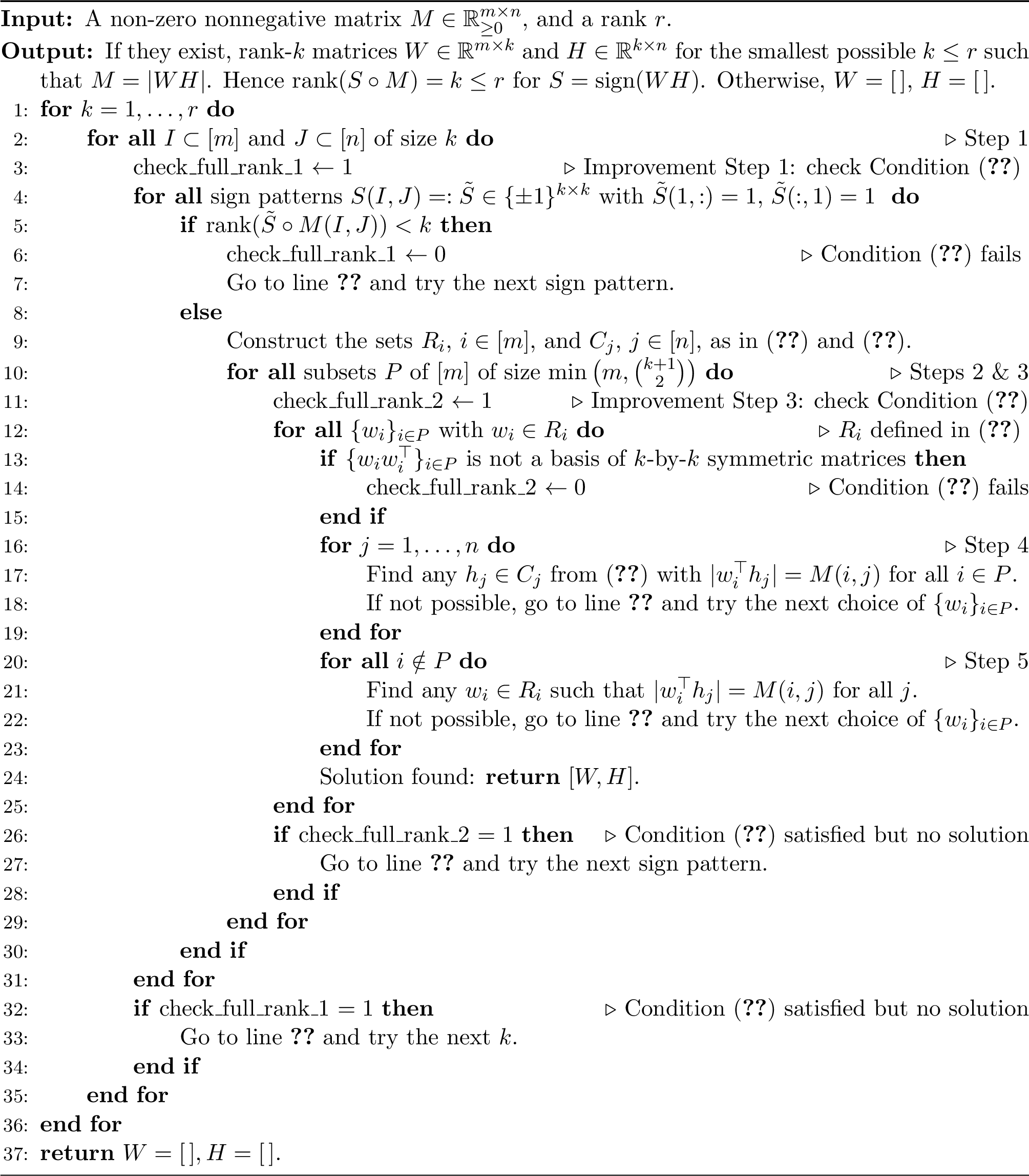
Step 1: Choosing a nonsingular basis block. Enumerate all pairs \((I,J)\) with \(I\subseteq[m]\), \(J\subseteq[n]\), \(|I|=|J|=k\), and all sign patterns \(S(I,J) \in\{\pm1\}^{k\times k}\) for \(k \in [r]\). Set \(Y(I,J) = S(I,J) \circ M(I,J)\), but discard the branch if \(Y(I,J)\) is singular. In summary, after this step, we have fixed the sign pattern of a \(k\)-by-\(k\) sub-matrix of \(S\) indexed by \((I,J)\) such that \(Y(I,J) = S(I,J) \circ M(I,J)\) is non singular. The number of branches at Step 1 is at most \(\binom{m}{k}\binom{n}{k}2^{k^2}\leq \mathcal{O}\bigl((mn)^r\,2^{r^2}\bigr)\).
Step 2: Column and row candidates. For a branch with a \(k\times k\) nonsingular sub-matrix \(Y(I,J)\) indexed by \((I,J)\), any compatible rank-\(k\) matrix may use the columns indexed by \(J\) as a basis of its column space, that is, \(W = Y(:,J)\). Let us denote \(w_i^\top \in \mathbb{R}^r\) the \(i\)th row of \(W \in \mathbb{R}^{m \times r}\) for \(i\in[m]\). We know \(W(I,:) = Y(I,J)\) since these signs have been fixed. For the other rows of \(W\), we can still pick any signs for \(Y(i,J)\) for \(i \notin I\), with a total of \(2^k\) possibilities for each row. In summary, for all \(i\in[m]\), \[\label{eq:setsRi} w_i \; \in \; R_i \;=\; \begin{cases} \bigl\{u\in\mathbb{R}^{k}:|u|=M(i,J)^\top \bigr\} & \text{ for }i\notin I,\\[4pt] \{ Y(i,J)^\top \} & \text{ for } i \in I. \end{cases}\tag{3}\] Similarly, for the \(j\)th column of \(H \in \mathbb{R}^{r \times n}\), denoted \(h_j\), we have, using the Skeleton decomposition, \[\label{eq:setsCi} h_j \; \in \; C_j \; = \; \begin{cases} \bigl\{Y(I,J)^{-1} y : y\in\mathbb{R}^{k},\;|y|=M(I,j)\bigr\} & \text{ for } j\notin J,\\[4pt] \{e_{\ell}\} & \text{ for } j \in J \text{ and j is the \ellth entry in J}. \end{cases}\tag{4}\] Note that \(H(:,J) = I_k\), the \(k\)-by-\(k\) identity matrix.
Suppose that a feasible rank-\(k\) matrix \(Y = S \circ M\) exists, where \(S(I,J)\) was fixed (Step 1). By the skeleton decomposition, there must exist vectors \(w_i\in R_i\) and \(h_j \in C_j\) such that \(Y(i,j) = w_i^\top h_j\) for all \(i,j\), hence \(|Y(i,j)| = M(i,j) = |w_i^\top h_j|\) for all \(i,j\). Finding the candidates \(w_i\in R_i\) and \(h_j \in C_j\) such that \(M(i,j) = |w_i^\top h_j|\) for all \((i,j)\) hence provides a certificate that a feasible solution is found (if such candidates do not exist, then one cannot play with the signs of \(M\) to make it rank \(k\)). Unfortunately, checking all candidates does not lead to the desired results (namely, having an algorithm polynomial in \(m\) and \(n\)), as for each of the remaining \(m-k\) rows (resp.\(n-k\) columns) of \(S\), there are \((2^k)^{m-k}\) (resp.\((2^k)^{n-k}\)) candidates. The next step will select a sufficiently small subset of the row candidates to achieve our goal.
Step 3: Selecting row candidates. For any feasible choice of row and column candidates \(w_i \in R_i\) and \(h_j \in C_j\) for all \((i,j)\), the feasibility condition \(|w_i^\top h_j|=M(i,j)\) between row \(i\) and column \(j\) can be rewritten as \[\label{eq:linearxxuu} \langle h_j h_j^\top,\,w_i w_i^\top\rangle = M(i,j)^2.\tag{5}\] The matrices \(w_iw_i^\top\) lie in the space of \(k\times k\) symmetric matrices, whose dimension is \(\binom{k+1}{2}\). Hence, there exists \(P\subseteq[m]\) with \(|P|\leq\binom{k+1}{2}\) such that \(w_\ell w_\ell^\top\) lies in the linear span of \(\{w_iw_i^\top:i\in P\}\) for all \(\ell\in[m]\). Note that if \(m \leq \binom{k+1}{2}\), we can simply pick all rows and then keep only the corresponding linearly independent matrices. This linear dependence will allow us in the next step (Step 4) to determine the row candidates of \(W\) for \(i \notin P\) given the row candidates \(i \in P\). In order to identify if a matrix \(Y\) exists, we branch over all possible subsets \(P\) of size \(\min\big(m, \binom{k+1}{2}\big)\) and all possible choices of \(w_i\in R_i\) for \(i\in P\), creating at most \[\binom{m}{\binom{k+1}{2}}(2^k)^{\binom{k+1}{2}} = m^{\mathcal{O}(k^2)}\,2^{\mathcal{O}(k^3)} \leq m^{\mathcal{O}(r^2)}\,2^{\mathcal{O}(r^3)}\] different new branches to explore. Note that we do not check whether \(\{w_iw_i^\top\}_{i \in P}\) spans \(\{w_iw_i^\top\}_{i \in [m]}\) for all possible \(w_i \in R_i\) since this would be too expensive: what is important is that at least one such \(P\) will be such that \(\{w_iw_i^\top\}_{i \in P}\) spans \(\{w_iw_i^\top\}_{i \in [m]}\). However, the algorithm might find a solution for a \(P\) that does not satisfy this condition.
Step 4: Filtering column candidates. In step 3, we identified the candidates \(w_i\in R_i\) for \(i\in P\), each of which we can explore as a new branch (since there are sufficiently few, that is, a polynomial number in \(m\)). In other words, the subset of rows of \(W\) in \(P\) of size at most \(\binom{k+1}{2}\) is fixed and the candidate \(w_i\) is selected for all \(i \in P\). We use them to check which column candidates for \(H\) remain compatible with the candidate rows for \(W\). For each \(j\in[n]\), we retain only the candidates \(h_j \in C_j\) satisfying \((w_i^\top h_j)^2=M(i,j)^2\) for all \(i\in P\). We discard the branch if no candidate \(h_j \in C_j\) satisfies these conditions for some \(j\), otherwise we select arbitrarily one surviving candidate per column. The justification for keeping an arbitrary survivor is given in the next step.
Step 5: Selecting the remaining row candidates. At the end of Step 4, one candidate \(h_j\in C_j\) has been selected for every column \(j\in[n]\). It remains to select the row candidates \(w_i\in R_i\) for \(i\notin I\cup P\). By construction, the selected \(h_j\)’s satisfies \[\langle h_jh_j^\top,w_i w_i^\top\rangle=M(i,j)^2 \qquad\text{for all }i\in P.\] For each \(i\notin I\cup P\), we select the vectors \(w_i \in R_i\) satisfying \[(w_i^\top h_j)^2=M(i,j)^2 \qquad\text{for every }j\in[n].\] If no candidate survives for some \(i\notin I\cup P\), we discard the branch. Otherwise, we select arbitrarily one surviving candidate \(w_i\).
Let us show that the arbitrary choice of the \(h_j\)’s made in Step 4 are safe in a branch that leads to a feasible solution \(Y\). Let \(h_j^\ast\) be another admissible choice for column \(j\) in Step 4, that is, this column coordinate \(h_j^\ast\) satisfies \[\langle h_j^\ast (h_j^\ast)^\top,w_i w_i^\top\rangle = M(i,j)^2 = \langle h_jh_j^\top,w_i w_i^\top\rangle \qquad\text{for all }i\in P.\] For \(\ell\in[m]\), if \(\{w_i w_i^\top\}_{i \in P}\) spans \(\{w_i w_i^\top\}_{i \in [m]}\), there exist scalars \(\alpha_i\) such that \(w_\ell w_\ell^\top =\sum_{i\in P}\alpha_i\,w_i w_i^\top\). Therefore, \[\begin{align} \langle h_jh_j^\top,w_\ell w_\ell^\top\rangle = \sum_{i\in P}\alpha_i\langle h_jh_j^\top,w_iw_i^\top\rangle = \sum_{i\in P}\alpha_i M(i,j)^2 = \sum_{i\in P}\alpha_i\langle h_j^\ast (h_j^\ast)^\top,w_i w_i^\top\rangle & = \langle h_j^\ast (h_j^\ast)^\top,w_\ell w_\ell^\top\rangle \\ & = M(\ell,j)^2. \end{align}\] This means that the choice of any admissible \(h_j\) in Step 4 does not affect the value of \(\langle h_jh_j^\top, w_\ell w_\ell^\top\rangle\) for all \(\ell \in [m]\), because of the linear dependence.
Step 6: Constructing the factorization. If there were no rank-\(k\) feasible solution \(Y = S \circ M\), then no branch generated in Steps 1-5 will remain, and we can conclude that the rank-\(k\) problem is not feasible. Otherwise, our procedure provides a rank-\(k\) factorization \((W,H)\) such that \(M = |WH|\). In fact, let \(W\) and \(H\) contain the selected row and column candidates, respectively, that is, \[W=\begin{pmatrix}w_1^\top\\\vdots\\w_m^\top\end{pmatrix} \in\mathbb{R}^{m\times k}, \qquad H= \begin{pmatrix}h_1&\cdots&h_n\end{pmatrix} \in\mathbb{R}^{k\times n}, \quad\text{ and }\quad S=\operatorname{sign}(WH)\in\{\pm 1\}^{m\times n}.\] By the filtering performed in the previous steps, the selected candidates satisfy \(|W(i,:)\,H(:,j)|=|w_i^\top h_j|=M(i,j)\) for every \(i\in[m]\) and \(j\in[n]\), so \(\operatorname{rank}(S\circ M)= \operatorname{rank}(WH)\le k\leq r\).
Running time. For each \(k\le r\), Step 1 produces \(\mathcal{O}\bigl((mn)^k\,2^{k^2}\bigr)\) branches and Step 3 produces \(m^{\mathcal{O}(k^2)}\,2^{\mathcal{O}(k^3)}\) further branches. Steps 4–5 cost \(\operatorname{poly}(m,n)\) per branch. The total is3 \((mn)^r\cdot m^{\mathcal{O}(r^2)}\cdot 2^{\mathcal{O}(r^3)}\cdot\operatorname{poly}(m,n,r)\). This concludes the proof.
Note that the term \(m^{\mathcal{O}(r^2)}\) comes from the fact the we first explore the possible signs of the rows of \(W\) in the sets \(R_i\)’s. If \(n < m\), it is preferable to apply the algorithm on the transpose to have complexity \(n^{\mathcal{O}(r^2)}\). ◻
3.2 Improvements of the algorithm and FPT for generic matrices↩︎
In this section, we first provide two general improvements of the algorithm described in Theorem 3, one for Step 1 in Sections 3.2.1 and one for Step 3 in Section 3.2.2. This allows us to provide a fixed-parameter tractable (FPT) algorithm in the parameter \(r\) for rank-\({r_\star}\) generic matrices, where \({r_\star}\) is a fixed positive integer, with probability one (w.p.1) in Section 3.2.3.
3.2.1 Improvements of Step 1↩︎
We have the following result.
Lemma 2. Given \(1\leq k\leq r\), let us consider Step 1 of the algorithm described in Theorem 3. Assume we have found a pair of subsets \((I,J)\) with \(|I|=|J|=k\) such that \[\label{eq:condStep1} \rank\Big( M(I,J) \circ S(I,J) \Big) = k \quad \text{ for all } \quad S(I,J) \in \{\pm 1\}^{k \times k}.\qquad{(1)}\] Then one does not need to consider other pairs of subsets \((I,J)\) to guarantee whether there exists \(S\) such that \(\rank(M \circ S) \leq k\).
Proof. The condition ?? means that, regardless of its sign pattern, the sub-matrix \(M(I,J)\) always has rank \(k\), that is, we cannot reduce its rank by playing with its signs. This implies that, regardless of the sign pattern \(S\), we can always construct a Skeleton approximation using the indices \((I,J)\) since \(S(I,J) \circ M(I,J)\) is invertible for all sign pattern \(S(I,J)\), and hence we do not need to explore other subsets of indices in the algorithm described in Theorem 3 that construct a Skeleton approximation of \(Y = M \circ S\). ◻
As we will see in Section 3.2.3, condition ?? is valid w.p.1 for generic matrices, and hence only one subset of indices \((I,J)\) needs to be checked in that case, leading to an FPT complexity in the parameter \(r\) for Step 1.
Another improvement for Step 1 (line [setp:signpattern] in Algorithm 2), is that not all sign patterns need to be checked for \(M(I,J)\). In fact, the rank of a matrix is unchanged under sign flips of its rows and columns, hence we can assume w.l.o.g.that the first row and first column of \(S(I,J)\) have a fixed sign pattern, e.g., \(\tilde{S}(1,:) = \tilde{S} (:,1) = 1\) where \(\tilde{S} := S(I,J)\). This means that we only need to check \(2^{(k-1)^2}\) sign patterns instead of \(2^{k^2}\).
3.2.2 Improvement of Step 3↩︎
The other step that is not FPT in Theorem 3 is Step 3. Recall that, in Step 3, we need to check all subsets \(P\) of size \(\min\big(m,\binom{k}{2}\big)\) of rows of \(W\), for \(1\leq k \leq r\). In a similar spirit as for Step 1, if for a subset \(P\), \(\{w_i w_i^\top\}_{i \in P}\) is a basis of the symmetric matrices for any possible choice of the signs (that is, for any \(w_i \in R_i\)), we do not need to consider other subsets.
Lemma 3. Given \(1\leq k\leq r\), let us consider Step 3 of the algorithm of Theorem 3. Assume that the subset \(P\) of size \(\min\big(m,\frac{k(k+1)}{2}\big)\) is such that \[\label{eq:condStep3} \{w_iw_i^\top\}_{i \in P} \text{ are linearly independent for all } w_i \in R_i.\qquad{(2)}\] Then, in the algorithm of Theorem 3, one does not need to consider other subsets \(P\) in Step 3 for the current sign pattern \(S(I,J)\).
Proof. Since \(\{w_iw_i^\top\}_{i \in P}\) are linearly independent regardless of the choice of the \(w_i\)’s in \(R_i\), all other rank-one matrices, \(\{w_iw_i^\top\}_{i \notin P}\), will be in the span of \(\{w_iw_i^\top\}_{i \in P}\). Hence, when looking for \(h_j \in C_j\) in Step 5, the argument described in Step 5 allows us to only check the conditions \(\langle h_jh_j^\top,w_i w_i^\top\rangle=M(i,j)^2\) for \(i\in P\), as it will imply \(\langle h_jh_j^\top,w_i w_i^\top\rangle=M(i,j)^2\) for \(i\notin P\). ◻
As we will see in Section 3.2.3, condition ?? is valid w.p.1 for generic matrices, and hence only one set \(P\) needs to be checked in that case, leading to an FPT complexity in the parameter \(r\) for Step 3.
Algorithm 2 provides the pseudo-code of the algorithm described in Theorem 3, combined with the improvements in Steps 1 and 3 described in the two previous sections, which stop the algorithm early when ?? is satisfied, or avoid enumerating all subsets \(P\) for a given sign pattern \(S(I,J)\) when ?? is satisfied.
3.2.3 Fixed-parameter tractable algorithm for generic matrices↩︎
For simplicity, we consider generic matrices of the following form: the matrix \(Y\) is a generic rank-\({r_\star}\) matrix if \(Y = W_{\#} H_{\#}\), where the entries of \(W_{\#} \in \mathbb{R}^{m \times {r_\star}}\) and \(H_{\#} \in \mathbb{R}^{{r_\star}\times n}\) are drawn from a continuous distribution (e.g., Gaussian or uniform).
Before proving that Algorithm 2 is fixed-parameter tractable (FPT) in the parameter \(r\) for such generic rank-\({r_\star}\) matrices (Theorem 4), we provide several lemmas. The first lemma shows that for a generic rank-\({r_\star}\) matrix \(Y\), the \(k\)-by-\(k\) sub-matrix \(Y(I,J) \circ \tilde{S}\) is full rank w.p.1 for any sign pattern \(\tilde{S}\) and any \(1 \leq k \leq {r_\star}\).
Lemma 4. Let \(Y=W_{\#}H_{\#}\), where the entries of \(W_{\#} \in \mathbb{R}^{m\times {r_\star}}\) and \(H_{\#} \in \mathbb{R}^{{r_\star}\times n}\) are drawn from a continuous distribution. Then \[\label{eq:sumprobzero} \sum_{k=1}^{r_\star}\sum_{\substack{S\in \{\pm 1\}^{m\times n} \\ I \subset [m],J\subset [n]: |I|=|J|=k}} \mathbb{P}\left( \det\big( S(I,J)\circ Y(I,J) \big)=0 \right) \quad = \quad 0,\qquad{(3)}\] which means that for all \(k\), for every choice of the matrix \(S\) and of the sets \(I\) and \(J\) of size \(k\), the sub-matrix \(S(I,J)\circ Y(I,J)\) has full rank w.p.1.
Proof. Since the sum in ?? runs on a finite set, it is enough to show the claim for \(k\), \(S\), \(I\) and \(J\) fixed. The polynomial \[{f}(W(I,:),H(:,J)) = \det(S(I,J)\circ W(I,:)H(:,J))\] is non-zero, since for the choice \(W(I,:)= I \circ S\) and \(H(:,J)=I\) it has value \(1\). Then the claims follows from the fact that the set of the zeros of \({f}\) has measure zero, and the fact that \(W_{\#}\) and \(H_{\#}\) are picked from a continuous distribution. ◻
The next two lemmas will be used to prove that \(\{w_i w_i^\top\}_{i \in P}\) form a basis of the set of symmetric matrices w.p.1 for generic input matrices. The first one shows that invertible linear transformations of a continuous distribution remains a continuous distribution.
Lemma 5. If a set of vectors \(\{w_1,\dots,w_\ell\} \in \mathbb{R}^d\) has an absolutely continuous joint distribution on \((\mathbb{R}^d)^\ell\), then for any \(q\leq d\) and for any fixed matrices \(B_1, \dots, B_\ell \in \mathbb{R}^{q \times d}\) with full row rank, \(\{B_1w_1,\dots, B_\ell w_\ell\}\) also has an absolutely continuous joint distribution on \((\mathbb{R}^q)^\ell\).
**Proof.* This is a consequence of a much more general statement about composition of Lebesgue measurable functions. For more details and the general statement, refer to [43]. ◻*
The second lemma provides the desired result regarding the span of \(\{w_i w_i^\top \}_{i \in P}\).
Lemma 6. Let \(Y = W_{\#}H_{\#}\), where the entries of \(W_{\#} \in \mathbb{R}^{m\times {r_\star}}\) and \(H_{\#} \in \mathbb{R}^{{r_\star}\times n}\) are drawn independently from a continuous distribution. The matrix \(M = |Y|\) is given as input to Algorithm 2. For any \(k \leq {r_\star}\), for any subset \(P \subseteq [m]\) of size \(N_k = \binom{k+1}{2}\), the matrices \(\{w_iw_i^\top\}_{i \in P}\) are linearly independent for all \(w_i \in R_i\), and hence they span the entire space of \(k \times k\) symmetric matrices w.p.1.
**Proof.* Let \(P\) be any subset of \([m]\) of size \(N_k = \binom{k+1}{2}\). For the simplicity of exposition, without loss of generality, we assume \(P = \{1,\dots,N_k\}\). Define the map \[\phi:\mathbb{R}^k \to \mathbb{R}^{N_k}, \qquad \phi(w)=\operatorname{svec}(ww^\top),\] where \(\operatorname{svec}\) denotes any vectorization of the independent entries of a symmetric matrix, that is, the values in the upper triangular part. The matrices \(\{w_iw_i^\top\}_{i=1}^{N_k}\) span \(\mathbb{S}^k\) if and only if the vectors \(\phi(w_1),\dots,\phi(w_{N_k})\) form a basis of \(\mathbb{R}^{N_k}\), that is, if and only if the matrix \[A= \begin{bmatrix} \phi(w_1)^\top\\ \vdots\\ \phi(w_{N_k})^\top \end{bmatrix} \in \mathbb{R}^{N_k\times N_k}\] is nonsingular. Since the entries of \(\phi(w)\) are quadratic polynomials in the entries of \(w\), the determinant \({f}(w_1,\dots,w_{N_k})=\det(A)\) is a polynomial in the entries of \(w_1,\dots,w_{N_k}\). Consider the following collection of \(N_k\) vectors: \[\mathcal{V} = \Big\{\frac{e_i+e_j}{2}, \text{ } 1\le i\leq j\le k\Big\}.\] Then the polynomial \({f}\) evaluated on these \(N_k\) vectors is non-zero and hence \({f}\) is not the zero polynomial. Since the entries of \(W_{\#}\) are picked independently at random from a continuous distribution, the vectors \(\{W_{\#}(i,:)^\top\}_{i \in P}\) have a joint continuous distribution in \((\mathbb{R}^{k})^{N_k}\). Following the definition in 3 , for some \(k \leq {r_\star}\), the row candidates \(w_i \in R_i\) are such that \(w_i = (W_{\#}(i,:)H_{\#}(:,J))^\top \circ s_i\) for some sign vector \(s_i \in \{\pm 1\}^k\) where \(J \subseteq [n]\), \(|J| = k\). For a fixed collection of sign vectors \(\{s_{1},\dots,s_{N_k}\} =: \sigma \in (\{\pm 1\}^k)^{N_k}\), taking \(D_i = \mathop{\mathrm{diag}}(s_i)\), we have \[\label{eq:relwiwiinp} w_i = D_iH_{\#}(:,J)^\top W_{\#}(i,:)^\top.\tag{6}\] By Lemma 5 for \(d = r_*\), \(q = k\) and \(\ell = N_k\), the corresponding candidate row vectors \(w_1,\dots, w_{N_k}\) have a joint continuous distribution. Hence, using the fact that the set of zeros of \(f\) has measure zero, \[\mathbb{P} \Big( f(w_1,\dots,w_{N_k}) = 0 \; \Big| \; \rank((D_i(H_{\#}(:,J))^\top) = k \Big) = 0.\] Since the entries of \(H_{\#}(:,J)\) are picked independently at random from a continuous distribution, \(\rank(D_i(H_{\#}(:,J))^\top)=k\) w.p.1, similarly as in Lemma 4. Using the fact that there are a finite number of \(\sigma\), using union bound, we can therefore conclude the matrices \(\{w_iw_i^\top\}_{i \in P}\) are linearly independent and hence, they span the entire space of \(k \times k\) symmetric matrices. ◻*
We can now prove that Algorithm 2 is FPT for generic input matrices.
Theorem 4. Given \({r_\star}\geq 1\), let \(M = |Y|\) where \(Y = W_{\#}H_{\#}\), such that the entries of \(W_{\#} \in \mathbb{R}^{m\times {r_\star}}\) and \(H_{\#} \in \mathbb{R}^{{r_\star}\times n}\) are drawn from a continuous distribution. Then Algorithm 2 run on \((M,r)\) for any \(r\) is FPT in parameter \(r\) as it runs in \(\mathcal{O}(2^{\tilde{r}^3}\cdot poly(m,n,\tilde{r}))\) operations, where \(\tilde{r} = \min(r, {r_\star})\).
Proof. If \(r \geq {r_\star}\), Algorithm 2 will terminate for \(k\leq {r_\star}\) since a feasible solution of rank \({r_\star}\) exists, otherwise the algorithm will stop for \(k\leq r\leq {r_\star}\). In all case, \(k\) will not exceed \(\tilde{r}\).
Now, for any \(k \leq \tilde{r}\), the two conditions ?? and ?? are satisfied w.p.1 for any \((I,J)\) and any \(P\), as shown in Lemmas 4 and 6. Hence, Algorithm 2 will only enter once the loop over the indices \((I,J)\) and over the subset \(P\), w.p.1. In the loop over \(P\), it might still need to check all possible \(w_i \in R_i\) for \(i \in P\), with at most \(2^{k^2(k+1)/2}\) different choices – there are \(k(k+1)/2\) vectors \(w_i \in \mathbb{R}^k\) whose entries can take two signs (unless \(i \in I\)); see 3 . Then
Checking linear independence of \(\{w_iw_i^\top\}_{i \in P}\) takes \(\mathcal{O}(k^6)\).
Finding \(h_j \in C_j\) such that \(|w_i^\top h_j| = M(i,j)\) takes up to \(2^k k \binom{k}{2}\) since \(C_j\) has up to \(2^k\) elements, the inner product costs \(k\) operations and there are \(\binom{k}{2}\) vectors \(w_i\). This has to be done \(n\) times.
Finding \(w_i \in R_i\) for \(i \notin P\) such that \(|w_i^\top h_j| = M(i,j)\) for all \(j\) takes up to \(2^k k n\) which has to be done \(m\) times.
Since when \(n>m\) it is always possible to consider \(Y^\top\), the total cost is \[\mathcal{O} \left( \tilde{r} 2^{\tilde{r}^3} ( \tilde{r}^6 + {\tilde{r}}^3 2^{\tilde{r}} \min(m,n) + \tilde{r} 2^{\tilde{r}} m n ) \right).\] ◻
We conclude this section with three remarks.
Remark 1 (Fixed-parameter linear). For generic matrices, Algorithm 2 is actually fixed-parameter linear in the parameter \(r\) since the computational cost is linear in the input size, \(mn\).
Remark 2 (Generic matrices). In this section, we considered rank-\(r\) generic matrices as the product of two smaller generic matrices. However, one could instead consider the more general case where the matrices are drawn from the manifold of rank-\(r\) matrices \(\mathcal{M}_r\). Although this space has zero ambient Lebesgue measure in \(\mathbb{R}^{m\times n}\) whenever \(r<\min\{m,n\}\), one can alternatively consider the restricted Hausdorff measure and then use that to define the notion of absolutely continuous probability measures on \(\mathcal{M}_r\) [44]. The proofs in this section generalize to that setting as well, but we use the current setting for the simplicity of the exposition.
Remark 3 (Last improvement of Algorithm 2). A drawback of Algorithm 2 is that it tries to find a rank-\(k\) solution, incrementing \(k\) from 1 to \(r\). Hence if the input matrix has a rank-\(r\) solution, but no smaller rank solution, it will first have to enumerate all \(k=1,2,\dots,r-1\) before finishing, which will be slow. To avoid this, one could start the iteration at \(k=r\), but then we do not necessarily have an FPT algorithm for generic matrices. Hence, in practice, it could actually be better to run two algorithms in parallel: one that increments \(k\) from 1, and the other that decrements from \(r\).
3.2.4 Implementation and numerical examples↩︎
We have implemented Algorithm 2 in MATLAB. It is available from
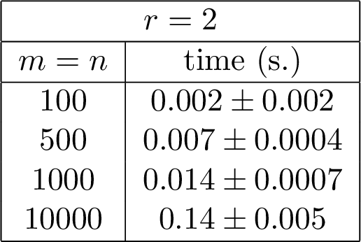
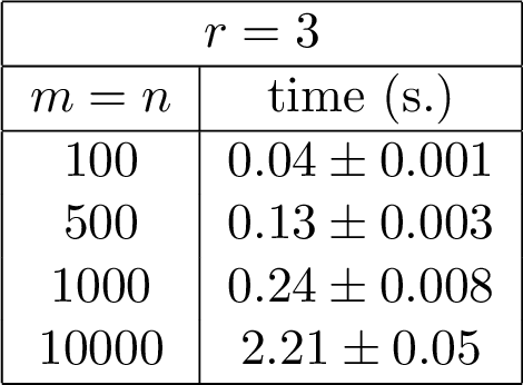
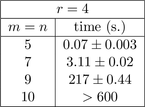
To give an idea of the size of matrices one can handle on a laptop4, Table [tbl:tab:runtime] reports the computational time needed for the algorithm to generate a feasible solution on rank-\(r\) randomly generated matrices. When there exists a feasible solution for \(r \in \{2,3\}\), our algorithm can handle matrices of large dimensions, up to \(10^4\), within seconds. For \(r=4\), the algorithm starts to stall. In fact, the largest term in the computational cost in Step 3, \(2^{(r-1)^3}\), goes from 256 for \(r=3\) to 134,217,728 for \(r=4\), so this quick change of behavior is expected.
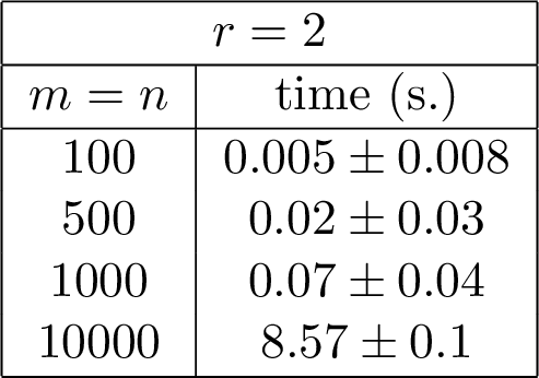
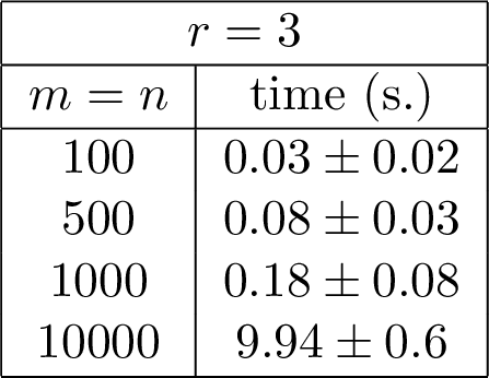
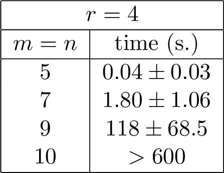
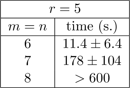
Table [tbl:tab:runtime2] reports experiments for full-rank generic matrices, to see how long the algorithm takes to certify that no rank-\(k\) solution exist for \(k \leq r\).
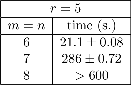
We observe two trends:
Algorithm 2 runs faster on full-rank matrices for \(r \in \{2,3\}\), especially as the dimension increases. For example, it takes Algorithm 2 about 8.5 seconds to process \(10^4\)-by-\(10^4\) generic matrices of rank 2, while 0.14 seconds to certify no rank-2 solution exist for full rank generic matrices of the same size. The reason is that when a feasible solution exists in the low-rank case, it has to construct it and go through all \(m\) rows of \(W\) and \(n\) columns of \(H\). In the full-rank generic case, even an \((r+1)\)-by-\((r+1)\) sub-matrix will not have a feasible rank-\(r\) solution, and hence the runtime of the algorithm is almost independent of \((m,n)\). It will not need to explore more than \(r+1\) rows and columns of \(W\) and \(H\) to decide for infeasibility.
For more difficult instances with \(r > 3\) and \(m,n\) close to \(r\), the full-rank matrices take typically more time to process. Algorithm 2 has to try all sign patterns for a given \((I,J)\) to make sure there is no feasible solution. It compensates for the fact that it may exit the loop over the set \(P\) earlier as observed above. While for low-rank matrices, it will stop as soon as a feasible solution is found. This also explains why the the standard deviation is close to zero for full-rank matrices: all sign patterns have to be checked since none are feasible. On the contrary, for low-rank matrices, there is randomness on how many patterns have to be tried before finding a feasible one. For example, for \(r=5\), \(m=n=7\), the shortest runtime for low-rank matrices over the 20 runs is 3.5 s and the longest is 315 s, while there are all about 286 s in the full-rank case.
3.3 Complexity of ExactEPMF↩︎
We can now prove that solving ExactEPMF for \(r\) fixed can be done in polynomial time, while, for the generic case when \(r\) is part of the input, the algorithm is FPT.
Corollary 2. Let \(p \in \mathbb{R}\), let \(X\in\mathbb{R}_{\geq0}^{m\times n}\), and let \(r\geq 1\) be fixed. There is a deterministic algorithm running in time polynomial in \(m\) and \(n\) that decides whether there exist matrices \(W\in\mathbb{R}^{m \times r}\) and \(H\in\mathbb{R}^{r \times n}\) such that \(X=|WH|^{\circ p}\), and outputs a solution if such a pair \((W,H)\) exists. Moreover, when \(r\) is a part of the input, the algorithm is FPT for generic input matrices.
Proof. Note that, for \(p < 0\), we must have \(X > 0\) otherwise there cannot exist \((W,H)\) such that \(X = |WH|^{\circ p}\). Set5 \(M=X^{\circ 1/p}\).
There exist \(W\in\mathbb{R}^{m\times k}\) and \(H\in\mathbb{R}^{k\times n}\) for some \(k\leq r\) such that \(X=|WH|^{\circ p}\) if and only if there exists a matrix \(Y\in\mathbb{R}^{m\times n}\) such that \[|Y|=M \qquad\text{and}\qquad \operatorname{rank}(Y)\leq r.\] Indeed, if \(Y=WH\), then \(|Y|^{\circ p}=X\). In the other way, if such a matrix \(Y\) exists, take any rank-\(k\) factorization \(Y=WH\) with \(W\in\mathbb{R}^{m\times k}\) and \(H\in\mathbb{R}^{k\times n}\). Thus, the problem is exactly the signing problem for the positive matrix \(M=X^{\circ 1/p}\), and the result follows from Theorems 3 and 4. ◻
The proof highlights the structural reason behind the fixed-rank tractability of ExactEPMF. Once a nonsingular basis block has been fixed, the remaining sign choices are not independent; they must satisfy a system of quadratic relations. The key point is that these conditions become linear when expressed in the space of symmetric \(k\times k\) matrices, whose dimension depends only on \(k\). Thus, although the number of possible sign choices is exponential in \(m,n\), only a bounded number of representative rows is needed to certify all constraints.
The next section shows that this tractability is specific to exact feasibility: once one considers the Frobenius-norm approximation problem, the fixed-rank problem becomes NP-hard already for \(r=2\).
4 NP-hardness of FroEPMF with \(r\) fixed↩︎
We now turn to the Frobenius-norm version of EPMF in the fixed-rank regime.
Definition 1 (Frobenius power factorization (FroEPMF)). Given a nonnegative matrix \(X\in\mathbb{R}_{\geq 0}^{m\times n}\) and an integer \(r\), the Frobenius absolute \(p\)-power factorization problem is \[\mathop{\mathrm{arg\,min}}_{W\in\mathbb{R}^{m\times r}, H\in\mathbb{R}^{r\times n}}\left\|X-|WH|^{\circ p}\right\|_F^2.\]
4.0.0.1 The rank-one case.
As for NMF, the rank-one case is elementary and can be solved in polynomial time. Indeed, when \(r=1\), writing \(W=w\in\mathbb{R}^m\) and \(H^\top=h\in\mathbb{R}^{n}\), we have \[|WH|^{\circ p}_{ij} = |w_i h_j|^p = |w_i|^p |h_j|^p.\] Thus, by setting \(a_i=|w_i|^p\) and \(b_j=|h_j|^p\), the rank-one FroEPMF problem is equivalent to \[\min_{a\in\mathbb{R}_+^m,\;b\in\mathbb{R}_+^n} \|X-ab^\top\|_F^2 .\] Since \(X\geq 0\), the best unconstrained rank-one approximation of \(X\) in Frobenius norm admits a nonnegative solution. The rank-one FroEPMF problem can be solved in polynomial time using the truncated SVD: let \((u,\sigma,v)\) be the first singular triplets of \(X\), then \(a = \sigma |u|\) and \(b = |v|\) is an optimal nonnegative solution, because \((X(i,j) - \sigma u_i v_j)^2 \geq (X(i,j) - \sigma |u_i| |v_j|)^2\) since \(X \geq 0\). Note that it could happen that \(a_i = 0\) for some \(i\), e.g., when \(X(i,:) = 0\) (and similarly for \(b_j\)). In this case and when \(p < 0\), the optimal solution is not attained, since \(w_i \rightarrow +\infty\) would be optimal. However, this does not happen when \(X X^\top\) and \(X^\top X\) are irreducible since the matrix then contains a positive singular pair by the Perron-Frobenius theorem. Note that, for \(p=0\), the problem is not interesting since \(|WH|^p\) is the all-one matrix for all \((W,H)\).
4.0.0.2 The rank-two case.
The main result of this section shows that the tractability of the rank-one case disappears immediately when \(r=2\). Our proof proceeds by a polynomial-time reduction from the decision version of the NP-hard Cut-Norm problem for sign matrices [5]. We begin by formally stating the decision versions of both problems.
Cut-Norm is NP-hard due to a polynomial-time reduction from the MAX-CUT problem [5]. Let us now reduce Cut-Norm to R2-FroEPMF in
polynomial-time. Given an instance \((M,D)\) of Cut-Norm, we construct an instance \((X,T)\) of R2-FroEPMF as follows:
\(N=\left\lceil\max\left\{(24p)^2(st)^3,(24p)^p(st)^{p+\frac{1}{2}} \right\}\right\rceil\),
\(T=\frac{st-D}{2}\),
\(m=s+2N\) and \(n=t+2N\),
\(X\in\{0,1,2^p\}^{m\times n}\) is defined as follows: \[X= \begin{pmatrix} B & \mathbf{1}_{s\times N} & \mathbf{1}_{s\times N}\\[1mm] \mathbf{1}_{N\times t} & 2^p \, \mathbf{1}_{N\times N} & \mathbf{0}_{N\times N}\\[1mm] \mathbf{1}_{N\times t} & \mathbf{0}_{N\times N} & 2^p \, \mathbf{1}_{N\times N} \end{pmatrix},\] with \[B=\frac{M+ \mathbf{1}_{s\times t}}{2}\in\{0,1\}^{s\times t}.\]
Theorem 5. The instance \((X,T)\) is a yes-instance of R2-FroEPMF if and only if \((M,D)\) is a yes-instance of CUT-NORM. Hence, R2-FroEPMF is NP-hard.
Proof. Let us denote \[I=\{1,\dots,s\},\quad R=\{s+1,\dots,s+N\},\quad R'=\{s+N+1,\dots,s+2N\},\] the indices of the three row blocks of \(X\), and \[J=\{1,\dots,t\},\quad C=\{t+1,\dots,t+N\},\quad C'=\{t+N+1,\dots,t+2N\},\] the indices of the three column blocks of \(X\).
4.0.0.3 If part.
Suppose first that \((M,D)\) is a yes-instance of CUT-NORM. It means that there exist \(u\in\{\pm1\}^s\) and \(v\in\{\pm1\}^t\) such that \(u^\top Mv\geq D\). We define \(W\in\mathbb{R}^{(s+2N)\times 2}\) and \(H\in\mathbb{R}^{2\times (t+2N)}\) as follows: \[W(i,:)= \begin{cases} (1,\,u_i), & i\in I,\\ (2,\,0), & i\in R,\\ (0,\,2), & i\in R', \end{cases} \qquad H(:,j)= \begin{cases} \tfrac{1}{2}(1,v_j)^\top, & j\in J,\\[1mm] (1,0)^\top, & j\in C,\\[1mm] (0,1)^\top, & j\in C'. \end{cases}\] In order to show that \(\|X-|WH|^{\circ p}\|_F^2 \leq T\), we examine the nine blocks of \(X\):
\(I\times J\): For \((i,j)\in I\times J\), we have \(W(i,:)=(1,u_i)\) and \(H(:,j)=\tfrac{1}{2}(1,v_j)^\top\) which gives \[W(i,:)H(:,j)=\frac{u_iv_j+1}{2}\in\{0,1\}.\] The objective function on \(X(I,J)\) is \[\begin{align} \|X(I,J)-|W(I,:)H(:,J)|^{\circ p}\|_F^2 & = & \sum_{i=1}^s\sum_{j=1}^t\left(\frac{M_{ij}+1}{2}-\frac{u_iv_j+1}{2}\right)^2\\ & = & \frac{1}{4}\sum_{i=1}^s\sum_{j=1}^t M_{i,j}^2-2u_iv_jM_{ij}+(u_iv_j)^2\\ & = & \frac{1}{4}\left(2st-2\sum_{i=1}^s\sum_{j=1}^tu_iv_jM_{ij}\right)\\ & = & \frac{st-\langle M,uv^\top \rangle}{2}. \end{align}\]
\(R\times C\) and \(R'\times C'\): the matrix \(|WH|^{\circ p}\) is equal to \(2^p\), hence \[\|X(R,C)-|W(R,:)H(:,C)|^{\circ p}\|_F^2=\|X(R',C')-|W(R',:)H(:,C')|^{\circ p}\|_F^2=0.\]
\(R\times C'\) and \(R'\times C\): the matrix \(|WH|^{\circ p}\) is equal to \(0\), hence \[\|X(R,C')-|W(R,:)H(:,C')|^{\circ p}\|_F^2=\|X(R',C)-|W(R',:)H(:,C)|^{\circ p}\|_F^2=0.\]
\(I\times C\), \(I\times C'\), \(R\times J\), \(R'\times J\): every inner product has absolute value \(1\), so \(|{\cdot}|^p=1\), matching the entries of \(X\) exactly.
Finally, \[\|X-|WH|^{\circ p}\|_F^2 = \frac{st-\langle M,uv^\top \rangle}{2} \leq \frac{st-D}{2} = T.\] Hence \((X,T)\) is a yes-instance of R2-FroEPMF.
The only if part. Suppose now that \((X,T)\) is a yes-instance of R2-FroEPMF, that is, there exist \(W\in\mathbb{R}^{m\times 2}\) and \(H\in\mathbb{R}^{2\times n}\) such that \[\label{eq:hypo-onlyif} \|X-|WH|^{\circ p}\|_F^2\leq T.\tag{7}\] We show that this implies that \((M,D)\) is a yes-instance of Cut-Norm. To do so, we exploit the repeated rows and columns of \(X\). For a fixed \(H\), all rows \(X(i,:)\) with \(i\in R\) are the same; hence, we may choose all the rows \(W(i,:)\), \(i\in R\), to be equal in an optimal solution. The same argument applies to the rows indexed by \(R'\), and symmetrically to the columns indexed by \(C\) and \(C'\). Hence, without loss of generality, we may assume that \((W,H)\) has the form \[\label{eq:solonlyif} W= \begin{pmatrix} a&a'\\ r_1\mathbf{1}_N & r_2\mathbf{1}_N\\ r'_1\mathbf{1}_N & r'_2\mathbf{1}_N \end{pmatrix}, \qquad H= \begin{pmatrix} b&b'\\ c_1\mathbf{1}_N&c_2\mathbf{1}_N\\ c'_1\mathbf{1}_N&c'_2\mathbf{1}_N \end{pmatrix}^\top,\tag{8}\] for some \(a,a'\in\mathbb{R}^s\), \(b,b'\in\mathbb{R}^t\), and \(r_1,r'_1,r_2,r'_2,c_1,c'_1,c_2,c'_2\in\mathbb{R}\). From this solution of the R2-FroEPMF instance, we construct a solution of the Cut-Norm instance. We define \(u\in\{\pm1\}^s\) and \(v\in\{\pm1\}^t\) using the signs of \(a\) and \(b\): \[\label{eq:def95sigma95tau} u_i= \begin{cases} +1,& \text{when~~} a_ia'_i\geq 0,\\ -1,& \text{when~~} a_ia'_i<0, \end{cases} \quad v_j= \begin{cases} +1,& \text{when~~} b_jb'_j\geq 0,\\ -1,& \text{when~~} b_jb'_j<0. \end{cases}\tag{9}\] It remains to prove that with this solution \((u,v)\) and the hypothesis 7 , we have \(\langle M,uv^\top \rangle\geq D\).
We now decompose the objective according to four parts of \(X\), following the division \([s+2N]=I\cup \widetilde{R}\) and \([t+2N]=J\cup \widetilde{C}\), where \(\widetilde{R}=R\cup R'\) and \(\widetilde{C}=C\cup C'\): \[\|X-|WH|^{\circ p}\|_F^2 = E_{IJ}+E_{I\widetilde{C}}+E_{\widetilde{R}J}+E_{\widetilde{R}\widetilde{C}},\] where \(E_{IJ}\) is the contribution of the top-left block \(I\times J\), \(E_{I\widetilde{C}}\) is the contribution of the top-right blocks \(I\times \widetilde{C}\), \(E_{\widetilde{R}J}\) the contribution of the bottom-left blocks \(\widetilde{R}\times J\), and \(E_{\widetilde{R}\widetilde{C}}\) the contribution of the bottom-right blocks \(\widetilde{R}\times \widetilde{C}\). Note that since \[T=\frac{st-D}{2}\leq st,\] we have \(\|X-|WH|^{\circ p}\|_F^2\leq T \leq st\).
Step 1: the \(\widetilde{R} \times \widetilde{C}\) bottom-right block constrains \(r_1,r_1',r_2,r_2',c_1,c_1',c_2,c_2'\). We first analyze the four \(N\times N\) blocks in the bottom-right corner. Their contribution is \[\begin{align} E_{\widetilde{R}\widetilde{C}} & = & \|X(\widetilde{R},\widetilde{C})-|W(\widetilde{R},:)H(:,\widetilde{C})|^{\circ p}\|_F^2 \notag\\ &=& N^2\Bigl( (2^p-|r^\top c|^p)^2 +|r^\top c'|^{2p} +|r'^\top c|^{2p} +(2^p-|r'^\top c'|^p)^2 \Bigr). \label{eq:EBR} \end{align}\tag{10}\] where \(r = [r_1,r_2]\), and similarly for \(r'\) and \(c\). Now suppose \(c'=\lambda c\) and fix \(x=|r^\top c|^p\), \(y=|r'^\top c|^p\), hence, using Lemma 8 with \(a=2^p\) and \(b=|\lambda|^p\), \[E_{\widetilde{R}\widetilde{C}} = N^2\Bigl( (2^p-x)^2 +|\lambda|^{2p}x^{2} +y^{2} +(2^p-|\lambda|^{p}y)^2 \Bigr) \geq 2^{2p}N^2,\] a contradiction. Since \(WH=(WS)(S^{-1}H)\) for any invertible matrix \(S\), we may assume \(c=(1,0)\) and \(c'=(0,1)\). Therefore \[\begin{align} E_{\widetilde{R}\widetilde{C}} & = & N^2\bigl((2^p-r_1^p)^2+|r_2|^{2p}+|r_1'|^{2p}+(2^p-{r_2'}^p)^2\bigr). \label{eq:EBR3} \end{align}\tag{11}\] Since all four terms in 11 are positive, each of them is strictly smaller than \(st\). Therefore, by denoting \(\varepsilon=\sqrt{st}/N<1\), we have \(r_1^p\in[2^p-\varepsilon,2^p+\varepsilon]\) and \(r_1\geq 1\) since \(r_1^p\ge 2^p-1\ge 1\) (the same holds for \(r_2'\)). Moreover, for \(\alpha,\beta\geq 1\), we have \(|\alpha^p-\beta^p|\geq |\alpha-\beta|\). Thus, \[r_1\in[2-\varepsilon,2+\varepsilon], \qquad r'_2\in[2-\varepsilon,2+\varepsilon].\] Since \(\varepsilon<1\), we also have \(\varepsilon\leq \varepsilon^{1/p}\). For simplicity, we use the weaker but uniform following bounds: \[\label{eq:boundparameters} r_1,~r'_2\in\left[2-\varepsilon^{\frac{1}{p}},2+\varepsilon^{\frac{1}{p}}\right], ~~~ r'_1,~r_2\in\left[-\varepsilon^{\frac{1}{p}},\varepsilon^{\frac{1}{p}}\right].\tag{12}\]
Step 2: the \(I\times\widetilde{C}\) and \(\widetilde{R}\times J\) side blocks constrain the entries of \(a,a',b,b'\). We analyze the two rectangular blocks \(I\times\widetilde{C}\): \[\begin{align} E_{I\widetilde{C}} & = & \|X(I,C\cup C')-|W(I,:)H(:,C\cup C')|^{\circ p}\|_F^2 = N\sum_{i=1}^s \Bigl((1-|a_i|^p)^2+(1-|a'_i|^p)^2\Bigr). \end{align}\] Since \(E_{I\widetilde{C}}\leq st\), \(\bigl||a_i|^p-1\bigr|\leq \sqrt{\frac{st}{N}}, \qquad \bigl||a'_i|^p-1\bigr|\leq \sqrt{\frac{st}{N}}\), that is, \[\label{eq:boundsa1a2} \bigl||a_i|-1\bigr|\leq \sqrt{\frac{st}{N}}, \qquad \bigl||a'_i|-1\bigr|\leq \sqrt{\frac{st}{N}}.\tag{13}\] In the same way, for the blocks \(R\times J\) and \(R'\times J\), \[\bigl||r_1 \mathbf{1}_N^\top b+r_1 \mathbf{1}_N^\top b'|^p-1\bigr|\leq \sqrt{\frac{st}{N}}, \quad \text{which gives } \bigl||r_1 \mathbf{1}_N^\top b+r_1 \mathbf{1}_N^\top b'|-1\bigr|\leq \sqrt{\frac{st}{N}}.\] and \[\bigl||r'_1 \mathbf{1}_N^\top b+r'_1 \mathbf{1}_N^\top b'|^p-1\bigr|\leq \sqrt{\frac{st}{N}}, \quad \text{which gives } \bigl||r'_1 \mathbf{1}_N^\top b+r'_1 \mathbf{1}_N^\top b'|-1\bigr|\leq \sqrt{\frac{st}{N}},\] Using these relations and the bounds 12 , we obtain, by Lemma 7 (see Appendix 6), the following bounds on \(|b_j|\) and \(|b'_j|\): \[\label{eq:boundsb1b2} \left| |b_j|-\frac{1}{2} \right|\leq \sqrt{N}\varepsilon+\varepsilon^{1/p}, \qquad \left||b'_j|-\frac{1}{2}\right|\leq \sqrt{N}\varepsilon+\varepsilon^{1/p}.\tag{14}\]
Step 3: the \(I\times J\) top-left block controls the disagreements between \(M\) and \(uv^\top\). We now turn to the block \(I\times J\). We distinguish the two types of disagreements between \(M\) and \(uv^\top\), in the sets \(F_0\) and \(F_1\) defined below, together with the two types of agreeing entries, in the sets \(F_2\) and \(F_3\): \[\begin{align} F_0&=&\{(i,j)\in I\times J:\;M_{ij}=-1,\;u_iv_j=1\},\\ F_1&=&\{(i,j)\in I\times J:\;M_{ij}=1,\;u_iv_j=-1\},\\ F_2&=&\{(i,j)\in I\times J:\;M_{ij}=1,\;u_iv_j=1\},\\ F_3&=&\{(i,j)\in I\times J:\;M_{ij}=-1,\;u_iv_j=-1\}. \end{align}\] The sets \(F_0\) and \(F_1\) are exactly the disagreement positions between \(M\) and \(uv^\top\), and we have \[\label{eq:disagreement95inner95product} \langle M,uv^\top\rangle = st-2(|F_0|+|F_1|).\tag{15}\] In the only-if direction, the factors 8 are supposed to be arbitrary. Thus, unlike in the construction of the if direction, we cannot assume that \(\tilde{a}_i:=(a_i,a'_i)^\top=(1,u_i)^\top\) and \(\tilde{b}:=(b_j,b'_j)^\top=\frac{1}{2}(1,v_j)^\top\) on the block \(I\times J\). However, we have seen that the side blocks force an approximate version of this structure: \(|a_i|\) and \(|a'_i|\) are close to \(1\), while \(|b_j|\) and \(|b'_j|\) are close to \(1/2\). Hence, the signs defined in 9 allow us to link the values \(|\tilde{a}_i^\top \tilde{b}_j|^p\) to the objective 15 . In the following, we decompose \(E_{IJ}\) over the four sets and remove the nonnegative contributions coming from the agreeing positions: \[\begin{align} E_{IJ} &= \sum_{(i,j)\in F_0} (0-|\tilde{a}_i^\top \tilde{b}_j|^p)^2 + \sum_{(i,j)\in F_1} (1-|\tilde{a}_i^\top \tilde{b}_j|^p)^2 + \sum_{(i,j)\in F_2} (1-|\tilde{a}_i^\top \tilde{b}_j|^p)^2 + \sum_{(i,j)\in F_3} (0-|\tilde{a}_i^\top \tilde{b}_j|^p)^2 \\ &\geq \sum_{(i,j)\in F_0} |\tilde{a}_i^\top \tilde{b}_j|^{2p} + \sum_{(i,j)\in F_1} (1-|\tilde{a}_i^\top \tilde{b}_j|^p)^2. \end{align}\] Now we have to bound \(|\tilde{a}_i^\top \tilde{b}_j|^p\) on \(F_0\) and \(F_1\). By denoting \(\eta:=\sqrt{\frac{st}{N}}+\left(\frac{\sqrt{st}}{N}\right)^{\frac{1}{p}}\) and using 13 ,14 , we have \[\label{eq:finalboundsab} \big| |a_i|-1\big| \leq \eta, \quad \left||b_j|-\frac{1}{2}\right|\leq \eta, \quad \big| |a'_i|-1\big| \leq \eta, \quad \text{ and } \quad \left||b'_j|-\frac{1}{2}\right|\leq \eta.\tag{16}\] Since \(N\geq (24p)^2(st)^3\), \[\sqrt{\frac{st}{N}} \le \sqrt{\frac{st}{(24p)^2(st)^3}} = \frac{1}{24pst}.\] Moreover, since \(N\ge (24p)^p(st)^{p+\frac{1}{2}}\), we get \[\left(\frac{\sqrt{st}}{N}\right)^{1/p} \le \left( \frac{\sqrt{st}}{(24p)^p(st)^{p+\frac{1}{2}}} \right)^{1/p} = \frac{1}{24pst}.\] Therefore \[\label{eq:boundetaonlypst} \eta = \sqrt{\frac{st}{N}} + \left(\frac{\sqrt{st}}{N}\right)^{1/p} \le \frac{1}{12pst}.\tag{17}\]
Let us analyze the indices in \(F_0\) and \(F_1\) separately:
For \((i,j)\in F_0\), \(u_iv_j=1\), hence both terms \(a_ib_j\) and \(a'_ib'_j\) have the same sign. Thus \[|\tilde{a}_i^\top \tilde{b}_j| = |a_ib_j+a'_ib'_j|=|a_ib_j|+|a'_ib'_j|\geq 2\left(1-\eta\right)\left(\frac{1}{2}-\eta\right)\geq 1-3\eta.\] By combining this bound on \(|\tilde{a}_i^\top \tilde{b}_j|\) with 17 , \[\label{eq:boundF0} |\tilde{a}_i^\top \tilde{b}_j|^p \geq (1-3\eta)^p\geq 1-3p\eta\geq 1 - \frac{1}{4st}.\tag{18}\]
For \((i,j)\in F_1\), \(u_iv_j=-1\); hence both terms \(a_ib_j\) and \(a'_ib'_j\) have opposite signs. Thus \[|\tilde{a}_i^\top \tilde{b}_j| = ||a_ib_j|-|a'_ib'_j||\leq (1+\eta)\left(\frac{1}{2}+\eta\right)-(1-\eta)\left(\frac{1}{2}-\eta\right)=3\eta.\] By combining this bound on \(|\tilde{a}_i^\top \tilde{b}_j|\) with 17 , \[\label{eq:boundF1} |\tilde{a}_i^\top \tilde{b}_j|^p \leq (3\eta)^p\leq \left(\frac{1}{4pst}\right)^p\leq \frac{1}{4st}.\tag{19}\]
By combining 18 and 19 , we obtain \[\begin{align} E_{IJ} &\geq \sum_{(i,j)\in F_0} |\tilde{a}_i^\top \tilde{b}_j|^{2p} + \sum_{(i,j)\in F_1} (1-|\tilde{a}_i^\top \tilde{b}_j|^p)^2\\ &\geq \left(1-\frac{1}{4st}\right)^2 |F_0|+\left(1-\frac{1}{4st}\right)^2 |F_1|\\ &\geq \left(1-\frac{1}{4st}\right)^2 \bigl(|F_0|+|F_1|\bigr) \geq \left(1-\frac{1}{2st}\right) \bigl(|F_0|+|F_1|\bigr). \end{align}\] Since \(E_{IJ}\leq T\), \(T\leq \frac{st}{2}\) and \(st\geq 1\), \[|F_0|+|F_1| \leq \frac{T}{1-\frac{1}{2st}}= T+\frac{\frac{T}{2st}}{1-\frac{1}{2st}} \leq T+\frac{\frac{1}{4}}{1-\frac{1}{2}} = T+\frac{1}{2}.\] Hence \[\langle M,uv^\top\rangle = st-2(|F_0|+|F_1|) > st - 2(T+\frac{1}{2}) \geq st - 2\frac{st-D}{2}-1=D-1.\] Since \(\langle M,uv^\top\rangle\) and \(D\) are integers, this implies \(\langle M,uv^\top\rangle\geq D\). ◻
5 Conclusion↩︎
In this paper, we studied the computational complexity of entrywise power matrix factorization (EPMF), a class of non-linear matrix decompositions (NMDs). We showed that EPMF is tractable in the exact fixed-rank regime, but otherwise it is NP-hard. For the exact fixed rank regime, we showed that the problem is equivalent to a signing problem: flip the signs of some entries of a given matrix to make it rank \(r\). We proposed a constructive algorithm polynomial in \((m,n)\) to solve this problem (Theorem 3). Moreover, we showed that the algorithm is FPT for generic matrices (Theorem 4). When the rank is not fixed, the problem is strongly NP-hard in the exact case (Corollary 1), and the least-squares optimization problem is already NP-hard for the smallest nontrivial rank, namely \(r=2\) (Theorem 5).
Further works include the study of conditions under which EPMF, and other NMDs, are tractable (e.g., using convexifications, or analyzing the loss landscape, as done for many low-rank matrix approximation problems), as well as the design of efficient algorithms and their use in real-world applications. We could also explore whether we can further reduce the computational cost of the algorithm that solves the sign problem in Theorem 3.
Use of AI assistance.
During the preparation of this manuscript, the authors used ChatGPT (OpenAI) to assist with improving the presentation of several proofs, exploring alternative proof strategies, and checking the clarity and logical consistency of mathematical arguments. The AI system was used solely as a writing and reasoning aid; all mathematical results, proofs, and conclusions were independently verified by the authors, who take full responsibility for the content of this manuscript.
6 Lemmas for the bounds on the coefficients around \(1/2\)↩︎
Lemma 7 (Bounds on the coefficients around \(1/2\)).
Let \(\varepsilon>0\), \(p>0\), \(N\geq 1\) such that \(\varepsilon^{\frac{1}{p}}< \frac{1}{2}\), and define \(\delta:=\sqrt{N}\varepsilon, \eta:=\varepsilon^{1/p}\). Let \(x_1,x_2\in\mathbb{R}\) be such that \[\big||(2+a)x_1+bx_2|-1\big|\leq \delta, \qquad \big||cx_1+(2+d)x_2|-1\big|\leq \delta,\] where \(a,b,c,d\in[-\eta,\eta]\). Then,for \(i=1,2\), \[\left||x_i|-\frac{1}{2}\right| \leq \delta+\eta, \quad \text{that is}, \quad \left||x_i|-\frac{1}{2}\right| \leq \sqrt{N}\varepsilon+\varepsilon^{1/p}.\]
Proof. From the assumptions, there exist signs \(\sigma_1,\sigma_2\in\{-1,1\}\) and errors \(e_1,e_2\) with \(|e_1|,|e_2|\leq \delta\) such that \[(2+a)x_1+bx_2=\sigma_1+e_1, \quad \text{and} \quad cx_1+(2+d)x_2=\sigma_2+e_2,\] which gives \[2\left(x_1-\frac{\sigma_1}{2}\right) = e_1-ax_1-bx_2 \quad \text{and} \quad 2\left(x_2-\frac{\sigma_2}{2}\right) = e_2-dx_2-cx_1.\] By using the bounds on the different elements, we obtain \[\label{eq:twoeqbounds} 2\left|x_1-\frac{\sigma_1}{2}\right| \leq \delta+\eta |x_1|+\eta |x_2| \quad \text{and} \quad 2\left|x_2-\frac{\sigma_2}{2}\right| \leq \delta+\eta |x_2|+\eta |x_1|.\tag{20}\] Set \[M:=\max_{i=1,2}\left|x_i-\frac{\sigma_i}{2}\right| \quad \text{and} \quad B:=\max_{i=1,2}\left|x_i\right| \quad \text{for which} \quad B\leq \frac{1}{2}+M.\] Using both equations of 20 , we obtain \(2M \leq \delta + 2\eta B \leq \delta + \eta + 2\eta M\), hence, \((2-2\eta)M \leq \delta+\eta\). Since \(\eta< 1/2\), for \(i=1,2\), \[\left||x_i|-\frac{1}{2}\right| \leq \left|x_i-\frac{\sigma_i}{2}\right| \leq M \leq \frac{\delta+\eta}{2-2\eta}\leq \delta+\eta.\] ◻
Lemma 8. Let \(a,b\in \mathbb{R}\). Then \[a^2 \; = \; \min_{x,y\in \mathbb{R}} (a-x)^2+b^2x^2+y^2+(a-by)^2.\]
**Proof.* Let \(f(x,y)=(a-x)^2+b^2x^2+y^2+(a-by)^2\). Then \[\nabla f(x,y)=\left(\begin{array}{c} -2(a-x)+2b^2x \\ 2y-2b(a-by) \\ \end{array}\right)= \left(\begin{array}{c} (2+2b^2)x-2a \\ (2+2b^2)y-2ab \\ \end{array}\right), \qquad \nabla^2 f(x,y)=\left(\begin{array}{cc} 2+2b^2 & 0 \\ 0 & 2+2b^2 \\ \end{array}\right),\] which means that \(f\) is strictly convex and attains the minimum when \(\nabla f=0\), that is at \(x_\star=\frac{a}{1+b^2}\) and \(y_\star=\frac{ab}{1+b^2}\). Hence \[f(x_\star,y_\star)=\left(a-\frac{a}{1+b^2}\right)^2+\frac{a^2b^2}{(1+b^2)^2}+\frac{a^2b^2}{(1+b^2)^2}+\left(a-\frac{ab^2}{1+b^2}\right)^2=\frac{a^2b^4+2a^2b^2+a^2}{(1+b^2)^2}=a^2.\] ◻*
References↩︎
Department of Mathematics and Operational Research. We acknowledge the support by the European Union (ERC consolidator, eLinoR, no 101085607). Emails: firstname.lastname@umons.ac.be.↩︎
SS is a member of the Gruppo Nazionale Calcolo Scientifico-Istituto Nazionale di Alta Matematica (GNCS-INdAM).↩︎
Moreover, for rational inputs, if the bit-size of the entries of \(M\) is at most \(b\), for \(r\) fixed, every rational number occurring in the computation has bit-size at most \(\text{poly}_r(b)\) and so the algorithm is strongly polynomial over \(\mathbb{Q}\).↩︎
Experiments performed with a 12th Gen Intel(R) Core(TM) i9-12900H 2.50 GHz, 32GB RAM, MATLAB R2019b.↩︎
Except for this step, the rest of the algorithm can be performed in the Blum-Shub-Smale (BSS) model of computation [45], [46]. To accommodate this step, we require oracle access to exact \(p\)th root computation for a fixed \(p\).↩︎