HamQASBench: A Hamiltonian-Informed Diagnostic Benchmark for Evaluating Quantum Architecture Search
July 06, 2026
Abstract
Quantum Architecture Search (QAS) automates the design of parameterized quantum circuits for variational quantum algorithms, yet existing benchmarks organize instances by molecular identity or qubit count—criteria agnostic to Hamiltonian structure—and rely solely on energy accuracy, which cannot detect structural failures such as over-parameterization on near-product ground states. We introduce HamQASBench, a Hamiltonian-informed diagnostic benchmark organizing 11 molecules into five structural tiers via fingerprints derived from the Pauli operator basis, computational basis representation, and ground-state entanglement. A post-hoc critical-structure extraction procedure identifies minimal circuits consistent with each tier’s requirements, complementing energy-based evaluation with per-qubit entanglement analysis and pairwise state fidelity. Benchmarking five QAS methods across four paradigms reveals failure modes invisible to conventional metrics: over-parameterization in the minimalism regime, eigenstate commitment under degeneracy, a representation bottleneck in strongly correlated systems, topology-induced routing failure, and circuit search space growth as a scalability bottleneck.
1 Introduction↩︎
In the noisy intermediate-scale quantum (NISQ) era [1], variational quantum algorithms (VQAs) have emerged as the leading paradigm for near-term quantum computation [2], [3]. Among these, the Variational Quantum Eigensolver (VQE) is particularly prominent for applications in quantum chemistry, where it is used to estimate molecular ground-state energies. Their effectiveness critically depends on the design of the underlying parameterized quantum circuit (PQC), or ansatz: a poorly chosen circuit structure lead to barren plateaus, insufficient expressivity, or excessive gate overhead [4], [5]. While fixed ansatz families such as hardware-efficient [6] and problem-inspired [7] templates have been proposed, they often require expert knowledge to construct and may generalize poorly across molecular instances and hardware configurations. These limitations motivate Quantum Architecture Search (QAS) [8]–[12], which aims to automatically discover circuit structures tailored to a given problem.
A central downstream task of QAS is ground-state energy estimation via VQE [2], [3], [13]: given a molecular qubit Hamiltonian \(H\), find a circuit \(C\) minimizing \(\langle C(\theta^*) | H | C(\theta^*) \rangle\), where solutions within 1.6 mHa of the true ground-state energy \(E_0\) are said to achieve chemical accuracy [13]. The quality of this estimate is therefore jointly determined by two factors: whether the circuit \(C\) is sufficiently expressive to represent the target ground state, and whether the classical optimizer can find suitable parameters \(\theta^*\) within that circuit. Critically, the structural requirements on \(C\) are not uniform across problem instances—they are governed by the properties of the Hamiltonian \(H\) itself [14], [15], which vary across molecular systems. For example, a diagonal-dominant Hamiltonian with near-zero ground-state entanglement admits a product-state solution representable by a handful of single-qubit rotations [16], [17], whereas a strongly correlated Hamiltonian with high single-qubit von Neumann entropy [15], [16] demands deep entangling structures spanning the full system. This instance-dependent complexity further underscores the need for automated approaches like QAS to design problem-adaptive circuit architectures. More importantly, existing QAS methods are typically evaluated on molecules organized by identity or qubit count [8]–[12], [18], [19]—criteria agnostic to these structural properties—and assessed solely on achieved energy, which cannot distinguish a method that learned the right structure from one that prepared a low-lying excited state with similar energy—a structural failure that propagates to downstream calculations such as excited-state spectra [20], dipole moments [21], and thermodynamic properties [22].
Concurrent benchmarking efforts such as BenchRL-QAS [23] and SQuASH [24] have advanced reproducibility and cross-method comparison, but organize molecules by task type or predefined search spaces rather than Hamiltonian structure, and provide no mechanism to assess whether discovered circuits are structurally consistent with the problem’s underlying quantum mechanical requirements. To address these limitations, we introduce HamQASBench, a Hamiltonian-informed diagnostic benchmark for QAS in variational ground-state energy estimation. Rather than selecting molecules by identity or system size, HamQASBench characterizes each molecule through Hamiltonian structural fingerprints derived from three complementary views of the qubit Hamiltonian: Pauli operator basis properties, computational basis representation, and energy and ground-state correlation structure. These fingerprints organize an 11-molecule, five-tier diagnostic suite spanning complementary structural regimes: minimalism, degeneracy, representation, topology, and same-family scalability. The final tier extends to 14-qubit systems via a GPU-accelerated optimization backend (see Section 8). To move beyond energy-only evaluation, we introduce a post-hoc critical-structure extraction procedure. This procedure iteratively prunes redundant gates from low-error training-stage circuits using counterfactual importance scoring, maintains a beam of candidate circuits under an energy tolerance constraint, and returns a minimal representation whose structure can be directly compared against each tier’s Hamiltonian fingerprints (see Section 3.1). We evaluate five representative QAS methods spanning four major paradigms—reinforcement learning [9], [10], differentiable relaxation [12], training-free filtering [18], and generative modeling [11]—and report cross-method findings invisible to conventional energy-only evaluation.
Our main contributions are as follows: 1) A structure-aware benchmark. HamQASBench organizes QAS evaluation around Hamiltonian structural fingerprints rather than molecular identity, enabling principled diagnosis of algorithmic behavior across complementary structural regimes. Molecule generation scripts, evaluation code, and extracted circuit data are publicly available at https://anonymous.4open.science/r/PSQASBench-D3D7. 2) A structural evaluation layer. The proposed post-hoc critical-structure extraction procedure identifies minimal circuit representations from training-stage circuits, providing a diagnostic signal orthogonal to energy accuracy. For non-degenerate instances, per-qubit von Neumann entropy comparison between pruned circuits and the exact ground state directly quantifies entanglement structure fidelity; for degenerate instances, pairwise state fidelity analysis reveals eigenstate commitment patterns invisible to energy metrics. 3) Cross-method diagnostic findings. Benchmarking five methods across four paradigms reveals qualitatively distinct failure modes—including over-parameterization, eigenstate commitment, entanglement mismatch, and topology-induced routing failure—demonstrating that energy accuracy alone is insufficient for diagnosing whether a QAS method has discovered a structurally appropriate circuit.
2 Related Work↩︎
2.0.0.1 Quantum Architecture Search.
QAS encompasses a broad range of methods for automatically discovering parameterized quantum circuit structures. Among the most studied, reinforcement learning approaches treat circuit construction as a sequential decision process: [19] pioneered curriculum-based RL for ansatz search, [9] extended this with structured state encodings and dynamic action masking, and [25] improved scalability via tensor-network warm-starting. [10] proposed HyRLQAS, jointly optimizing gate placement and parameter initialization under a hybrid discrete–continuous action space. Differentiable methods relax discrete gate selection into a continuous optimization problem [8], [12]. Sampling-based methods explore the circuit space by different mechanisms: supernet weight sharing over circuit subarchitectures [26], Monte Carlo tree search over gate sequences [27], and training-free proxy filtering over sampled candidate circuits [18]. Generative methods [11], [28] learn autoregressive models over gate sequences. Recent work has also explored block- and gadget-based search spaces [29], [30]. Despite this diversity, existing methods are evaluated on molecules organized by identity or qubit count and primarily on energy accuracy, leaving structural consistency with the underlying Hamiltonian unexamined.
2.0.0.2 Benchmarking QAS and Neural Architecture Search (NAS).
Early QAS benchmarking efforts focused on standardizing problem formulations: [31] proposed a benchmark based on randomly generated unitary targets, [23] systematically evaluated nine RL algorithms across multiple VQA tasks, and [24] leveraged surrogate models to accelerate evaluation across predefined search spaces. Inspired by the rapid growth of benchmarking in the classical NAS community—where tabular and surrogate benchmarks now cover diverse tasks and search spaces [32]–[35]—the QAS community has similarly recognized the need for principled evaluation. However, existing QAS benchmarks organize instances by task type, system size, or randomly generated targets, and primarily rely on energy-based metrics without probing structural consistency with the underlying Hamiltonian. HamQASBench fills this gap by grounding benchmark construction in Hamiltonian structural properties and introducing a structural evaluation layer orthogonal to energy accuracy.
2.0.0.3 Hamiltonian Structure and Ansatz Design.
The absence of structure-aware benchmarking is particularly striking given that several lines of work have established how Hamiltonian structure should inform ansatz design. From the Pauli operator basis perspective, [14] showed that the Hamiltonian Variational Ansatz, whose structure mirrors the Hamiltonian’s interaction terms, exhibits superior optimization properties. From the computational basis perspective, diagonal dominance governs ground-state proximity to a product state. By the Gershgorin circle theorem [36], strongly diagonal-dominant Hamiltonians confine eigenvalues near the diagonal entries; since computational basis states are product states, a ground state dominated by a single diagonal entry is well approximated by a product state, requiring only shallow circuits to represent [16]. Conversely, [17] established that circuits failing to respect the entanglement structure implied by the Hamiltonian exhibit trainability issues. From the ground-state entanglement perspective, [15] showed that ansatz construction guided by von Neumann entropy improves VQE performance, and [16] showed that entanglement mismatch impedes convergence. Together, these results establish Hamiltonian structural properties as principled predictors of circuit requirements, directly motivating the fingerprint design of HamQASBench.
3 Hamiltonian-Informed Diagnostic Benchmark↩︎
Existing empirical studies in QAS for variational ground-state energy estimation organize molecular instances by identity, qubit count, or conventional chemistry examples [8]–[12], [18], [19]—criteria agnostic to the structural properties of the underlying Hamiltonian. We instead construct HamQASBench around a set of Hamiltonian structural fingerprints, analyzing each molecule’s qubit Hamiltonian from three complementary perspectives: its Pauli operator basis structure, its computational basis representation, and the energy and correlation structure of its ground state.
3.1 Hamiltonian Structural Fingerprints↩︎
We derive a set of structural fingerprints from the qubit Hamiltonian across three complementary perspectives. The full theory from quantum chemistry principles are given in the Appendix 11. These fingerprints are used to organize the benchmark and are reported in Table ¿tbl:tab:hamiltonian95fingerprints?.
3.1.0.1 Pauli operator basis fingerprints.
We consider the Pauli expansion \(H = \sum_i c_i P_i\), where \(P_i\) are Pauli strings and \(c_i\) are their coefficients. This representation exposes operator composition and interaction structure: \(Z\)-only terms are diagonal, while \(X/Y\) terms are off-diagonal, inducing basis transitions and entanglement. From this view, we extract two indicators: \[r_Z = \frac{\sum_{P_i \in Z\text{-only}} |c_i|}{\sum_i |c_i|}, \quad r_{\ge 2} = \frac{\sum_{|P_i| \ge 2} |c_i|}{\sum_i |c_i|}.\] Here, \(r_Z\) measures proximity to a diagonal form, while \(r_{\ge 2}\) quantifies the weight carried by multi-qubit interaction terms—equivalently, \(r_{\ge 2} = 1 - r_{1\text{-body}}\), the complement of the single-qubit contribution.
3.1.0.2 Computational basis representation fingerprints.
We analyze the Hamiltonian in the computational basis, \(H = [h_{ij}]\), to capture diagonal dominance. Let \(R_i = \sum_{j \neq i} |h_{ij}|\). We define \[G_1 = \frac{1}{\dim(H)} \sum_i \mathbf{1}(|h_{ii}| \ge R_i), \quad G_2 = \min_{R_i > 0} \frac{|h_{ii}|}{R_i}.\] Here, \(G_1\) measures the fraction of diagonally dominant rows, while \(G_2\) captures the weakest diagonal dominance. This is illustrated in Fig. 1 b) as Gershgorin circles with centres \(h_{ii}\) and radius \(R_i\).
3.1.0.3 Energy and ground-state correlation fingerprints.
We characterize the spectral and correlation structure of the ground state through three quantities. The excitation gap \(\mathrm{Gap} = E_1 - E_0\) measures spectral separation between the ground state and the first excited state; when the ground state is degenerate, \(\mathrm{Gap} = 0\), and we explicitly annotate the degeneracy level (e.g., 2-fold or 3-fold) in Table ¿tbl:tab:hamiltonian95fingerprints? and Fig. 1a). The single-qubit von Neumann entropy [37]–[39] \[S(q) = -\mathrm{Tr}(\rho_q \log_2 \rho_q), \quad \rho_q = \mathrm{Tr}_{\bar q}(|\psi_0\rangle\langle\psi_0|),\] where \(\rho_q\) is the reduced density matrix of qubit \(q\) obtained from the exact ground state \(|\psi_0\rangle\), measures how entanglement is distributed across qubits and indicates the representation complexity of the target state. A value of \(0\) means the qubit is separable as shown in Fig. 1 c), with max value \(\ln(2)\).
Together, these fingerprints summarize three complementary perspectives on each instance: Pauli operator basis structure (\(r_Z\), \(r_{\ge2}\)), computational basis diagonal dominance (\(G_1\), \(G_2\)), and energy and ground-state correlation structure (\(\mathrm{Gap}\), degeneracy, \(S(q)\)).
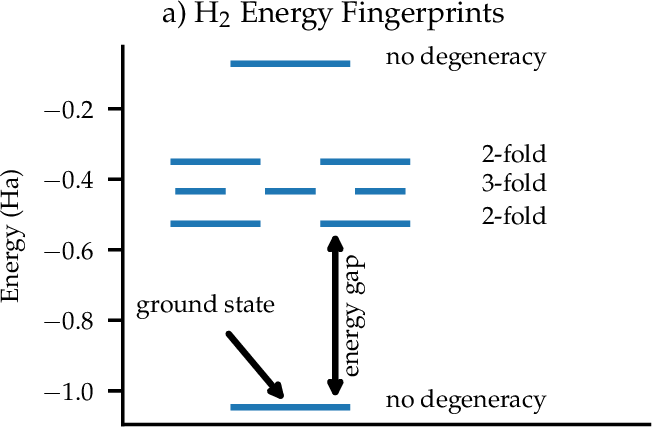
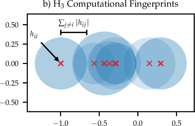
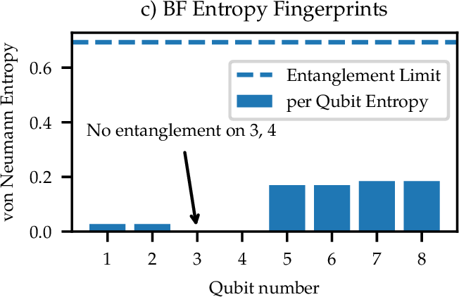
Figure 1: Visual illustration of Hamiltonian structural fingerprints for various molecules..
3.2 Diagnostic Tier Construction↩︎
Building on these Hamiltonian structural fingerprints, we construct a 5-tier diagnostic suite (Table ¿tbl:tab:hamiltonian95fingerprints?) through a combination of structure-driven grouping and instance selection. The selected molecules are curated to represent distinct structural regimes, and the resulting tiers are designed to probe complementary and largely orthogonal diagnostic pressures on QAS algorithms.
3.2.0.1 Tier 1: Minimalism.
Tier 1 targets strongly diagonal-dominant Hamiltonians (\(r_Z, G_1, G_2\) all high) with near-zero ground-state entanglement, for which product-state circuits are provably sufficient. BeH2_STO3G and
LiH_Equil represent this regime, with LiH_Equil offering a slightly harder case due to weaker diagonal dominance. This tier probes whether methods recover minimal structures or introduce unnecessary gates when a shallow solution
suffices.
3.2.0.2 Tier 2: Degeneracy.
Tier 2 isolates ground-state degeneracy as a diagnostic factor by selecting CH2, which exhibits three-fold degeneracy (\(\mathrm{Gap}=0\)) while remaining structurally simple in all other fingerprints (high
\(r_Z\), \(G_1\), low \(S(q)\)).1 This tier evaluates whether methods
converge to consistent circuit structures under non-unique optima, or drift across energetically equivalent solutions.
3.2.0.3 Tier 3: Representation.
Tier 3 targets the strong-correlation regime by selecting molecules with reduced diagonal dominance and high ground-state entanglement \(S(q)\). H2_Stretch serves as a tractable calibration case (\(G_1=0.75\), 4 qubits), while H2O_StrongCorr and H4_Chain (\(G_1=0.418\), \(r_{\ge2}=0.809\)) introduce heterogeneous and uniform strong
correlation at 8 qubits. This tier probes whether methods can faithfully encode strongly correlated ground states, and whether energy convergence implies correct entanglement structure.
3.2.0.4 Tier 4: Topology.
Tier 4 introduces hardware connectivity constraints by restricting two-qubit gates to nearest neighbours. H3_Linear is selected for its end-concentrated entanglement profile (\(S(q_0)=0.202\), \(S(q_5)=0.245\)), which requires long-range correlations that linear connectivity cannot directly implement. This tier evaluates whether methods can route entanglement effectively under topological constraints, independent of
correlation complexity.
3.2.0.5 Tier 5: Same-family scalability.
Tier 5 fixes molecular identity to BeH2 and increases basis set complexity across an 8–14 qubit ladder, so that \(r_Z\) decreases from \(0.953\) to \(0.767\) and \(G_1\) from \(0.980\) to \(0.621\) while ground-state entanglement remains controlled (\(S_{\max} \le 0.039\)). This isolates circuit search space growth as the sole variable, probing scalability independent of correlation complexity.
The resulting suite covers five complementary structural regimes, as summarized in Table ¿tbl:tab:hamiltonian95fingerprints?. Detailed molecular information is provided in Appendix 10.
width = , colspec = Q[30]Q[130]Q[15]Q[50]Q[50]Q[30]Q[30]Q[100]Q[450], cells = c, hline1, 2, 13 = -0.15em, Tier & Molecule & \(q\)
& \(r_Z\) & \(r_{\ge2}\) & \(G_1\) & \(G_2\) & \(\mathrm{Gap}\) (mHa)
& \(S(q)\)
Tier1 & BeH2_STO3G & 6 & 0.978 & 0.593 & 0.969 & 0.094 & 212 & [.008,.008,.005,.005,.005,.005]
Tier1 & LiH_Equil & 6 & 0.876 & 0.654 & 0.891 & 0.225 & 77 & [.018,.018,.006,.006,.013,.013]
Tier2 & CH2 & 8 & 0.907 & 0.483 & 0.945 & 0.21 & 0 (3-fold) & [.004,.004,.004,.070,.000,.000,.000,.068]
Tier3 & H2_Stretch & 4 & 0.728 & 0.849 & 0.75 & 0.18 & 4 & [.974,.974,.974,.974]
Tier3 & H2O_StrongCorr & 8 & 0.723 & 0.887 & 0.648 & 0.074 & 94 & [.021,.021,.342,.342,.316,.316,.071,.071]
Tier3 & H4_Chain & 8 & 0.599 & 0.809 & 0.418 & 0.011 & 233 & [.124,.124,.274,.274,.284,.284,.109,.109]
Tier4 & H3_Linear & 6 & 0.709 & 0.765 & 0.656 & 0.021 & 0 (2-fold) & [.202,.139,.147,.147,.083,.245]
Tier5 & BeH2_631G & 8 & 0.953 & 0.560 & 0.98 & 0.046 & 90 & [.024,.024,.002,.002,.002,.002,.021,.021]
Tier5 & BeH2_6311G & 10 & 0.923 & 0.533 & 0.963 & 0.01 & 63 & [.011,.011,.001(×4),.008,.008,.002,.002]
Tier5 & BeH2_CCPVDZ & 12 & 0.889 & 0.498 & 0.904 & 0.019 & 68 & [.022,.022,.002(×4),.012,.012,.003,.003,.008,.008]
Tier5 & BeH2_CCPVDZ & 14 & 0.767 & 0.700 & 0.621 & 0 & 61 & [.039,.039,.023,.023,.014(×4),.018,.018,.009,.009,.016,.016]
3.3 Post-hoc Critical-Structure Analysis↩︎
Energy alone is insufficient to determine whether a QAS method has learned circuit structures consistent with the Hamiltonian fingerprints. We therefore introduce a critical-structure extraction procedure that prunes redundant gates from training-stage circuits while preserving energy performance, isolating the minimal structure implied by each instance. Formally, we consider a set of snapshots \[\mathcal{S} = \{(C_i, \theta_i, \varepsilon(C_i,\theta_i))\}_{i=1}^N,\] where all circuits correspond to the same molecule and lie within a selected energy-error range. For each snapshot \((C_i, \theta_i, \varepsilon_i) \in \mathcal{S}\), we apply the following pruning procedure.
3.3.0.1 Gate importance.
For a circuit \(C\), we first re-optimize its parameters to obtain \(\varepsilon(C)\), and evaluate the counterfactual importance of each gate \(g_j \in C\) by \[\Delta_e(j) = \varepsilon(C \setminus g_j) - \varepsilon(C),\] which measures the performance degradation caused by removing \(g_j\).
3.3.0.2 Multi-branch pruning.
Instead of greedily removing the least important gate, we construct a sampling distribution inversely weighted by \(\Delta_e(j)\), where gates with smaller \(\Delta_e(j)\) are more likely to be removed. Starting from the original circuit, we iteratively expand a beam of candidate circuits by removing one gate at a time, while enforcing an energy tolerance constraint \(\varepsilon_{\mathrm{allow}}\).
Let \(\mathcal{B}_t\) denote the set of candidate circuits at iteration \(t\). For each \(C \in \mathcal{B}_t\), we generate candidates by removing one gate, i.e., \[\mathcal{N}(C) = \{ C \setminus g_j \mid g_j \in C,\; \varepsilon(C \setminus g_j) \le \varepsilon_{\mathrm{allow}} \},\] and construct the next set as \[\mathcal{B}_{t+1} = \mathrm{TopK}\big( \bigcup_{C \in \mathcal{B}_t} \mathcal{N}(C) \big),\] where \(\mathrm{TopK}(\cdot)\), i.e., a beam of fixed width, retains a fixed number of candidates with the smallest circuit size. This multi-branch exploration is necessary because gate contributions are not independent: removing one gate can change the importance of others due to parameter re-optimization and circuit-level coupling. The procedure iteratively expands candidate circuits and returns the smallest circuit that satisfies the error constraint, whose gate structure can be directly compared against each tier’s Hamiltonian fingerprints. Implementation details are provided in Appendix 12.
3.3.0.3 Structural consistency metrics.
Beyond energy, we assess structural consistency through two complementary metrics. For non-degenerate instances, we compute the per-qubit von Neumann entropy of each pruned circuit’s output state and compare it against the exact ground state: \[\mathrm{MAE}_S = \frac{1}{n}\sum_{q=1}^{n} |S_{\mathrm{circuit}}(q) - S_{\mathrm{exact}}(q)|,\] where \(S_{\mathrm{circuit}}(q)\) is obtained from the statevector of the re-optimized pruned circuit. A low \(\mathrm{MAE}_S\) indicates that the circuit faithfully reproduces the ground-state entanglement structure, not merely its energy. For degenerate instances, where the ground-state eigenspace contains multiple orthogonal states, we perform pairwise state fidelity analysis: \[F_{ij} = |\langle \psi_i | \psi_j \rangle|^2,\] clustering pruned circuits by fidelity threshold to identify which degenerate eigenstate each circuit targets, revealing eigenstate commitment patterns invisible to energy metrics.
4 Experimental Setup↩︎
4.1 Methods and Gate-Space Standardization↩︎
To systematically diagnose how different formulations of quantum architecture search behave in HamQASBench, we evaluate five representative methods spanning four major QAS paradigms: reinforcement learning [9], [10], differentiable optimization [12], sampling-based search [18], and generative modeling [11]. Rather than exhaustively covering the QAS literature, we select methods that capture distinct search mechanisms: sequential policy learning (CRLQAS, HyRLQAS), continuous architecture relaxation (QuantumDARTS), proxy-guided candidate filtering (TFQAS), and autoregressive circuit generation (GQEQAS).
To ensure that performance differences arise from search strategies rather than representational mismatches, we standardize the gate basis across all methods to \(\{\mathrm{RX}, \mathrm{RY}, \mathrm{RZ}, \mathrm{CNOT}\}\) while preserving each method’s native search mechanism. Table ¿tbl:tab:gate95standardization? summarizes the original gate pool, the pool used during benchmark search, the evaluation basis, and the stage at which each adaptation is applied. Detailed implementation choices are provided in Appendix 7.
width = , colspec = Q[120]Q[200]Q[200]Q[200]Q[180], cells = c, hline1, 2, 7 = -0.15em, Method & Original paper pool & Benchmark search pool & Eval.basis &
Adaptation stage
CRLQAS & {RX, RY, RZ, CNOT} & Same & Same & None
HYRLQAS & {RX, RY, RZ, CNOT} & Same & Same & None
QUANTUMDARTS & {Rz-Ry-Rz, I, CNOT} & Same & {RX, RY, RZ, CNOT} & Eval-time lowering
TFQAS & {RX, RY, RZ, XX, YY, ZZ} & {RX, RY, RZ, CNOT} & {RX, RY, RZ, CNOT} & Search-time replacement
GQEQAS & operator-pool-based & discretized gate-token pool & {RX, RY, RZ, CNOT} & Search-time replacement
4.2 Benchmark Configuration and Evaluation Protocol↩︎
4.2.0.1 Local optimizer and acceleration.
Circuit optimization is the primary bottleneck for scaling HamQASBench to larger systems, as training QAS models beyond 10 qubits requires repeated quantum-state simulation at each optimization step. We develop a GPU-enabled Optimizer Parallelization and Execution Backend that exploits batched circuit evaluation and parallel optimizer execution to accelerate parameter optimization. Under this backend, COBYLA [40] is used for systems up to 6 qubits for its robustness, while Rotosolve [41] is employed for larger systems due to its batched coordinate-sweep structure that enables efficient GPU acceleration. This configuration is critical for scaling the benchmark to the 10q–14q regime. Further details and empirical efficiency gains are provided in Appendix 8.
4.2.0.2 Circuit budget and connectivity variants.
For the Tier 1 molecule BeH2_STO3G and LiH_Equil, we evaluate under two maximum circuit depth budgets: Shallow (depth \(\le 10\)) and Deep (depth \(\le 50\)). This pair tests whether a method discovers a compact solution or overfills the available budget, which is the central diagnostic pressure of Tier 1. For Tier 4 (H3_Linear), we evaluate under two
connectivity settings: All (all-to-all two-qubit gates permitted) and Linear (nearest-neighbour only, 1D chain topology). This isolates the additional difficulty introduced by hardware connectivity constraints, independent of the
representational challenge of the underlying Hamiltonian.
4.2.0.3 Evaluation protocol.
For learning-based methods (RL, differentiable, and generative QAS), we perform periodic evaluation by sampling multiple circuits from the current model during training, providing a stable estimate of search quality while reducing variance from stochastic circuit sampling. TFQAS, which is training-free, directly produces a ranked set of candidate circuits on which evaluation is applied after final parameter optimization. For all methods, we report the best circuit found across the evaluation window, measured by energy error and CNOT count, ensuring a consistent comparison criterion across all QAS paradigms. Hyperparameters, training budgets, and the number of sampled circuits per evaluation are provided in Appendix 9.
5 Main Benchmark Results↩︎
Tables ¿tbl:tab:eval95results? and ¿tbl:tab:eval95results95t5? report the best circuits obtained across evaluation checkpoints for each method–molecule pair, measured by energy error (mHa), CNOT count, and rotation-gate count, with chemical accuracy (1.6 mHa) as the success threshold. In parallel, Table ¿tbl:tab:entropy95consistency? reports per-qubit von Neumann entropy consistency (\(\mathrm{MAE}_S\)) between pruned circuits and exact ground states for Tier 1 and Tier 3, providing a structural diagnostic orthogonal to energy accuracy. Training-stage best results and full structural analyses are reported in Appendix 13.1.
width = , colspec = Q[180]Q[120]Q[10]Q[10]Q[120]Q[10]Q[10]Q[120]Q[10]Q[10]Q[120]Q[10]Q[10]Q[120]Q[10]Q[10], cells = c, cell12 = c=30.157,
cell15 = c=30.161, cell18 = c=30.171, cell111 = c=30.165, cell114 =
c=30.167, cell82 = c=30.157, cell85 = c=30.161, cell88 = c=30.171,
cell811 = c=30.165, cell814 = c=30.167, hline1,2,8,9,15 = -0.15em, Molecule & T1_BeH2_6q (Shallow)
& & & T1_BeH2_6q (Depth) & & & T1_LiH_Equil_6q (Shallow) & & & T1_LiH_Equil_6q (Depth) & & & T2_CH2_8q & &
Method & Error & Cnot & Rot & Error & Cnot & Rot & Error & Cnot & Rot & Error & Cnot & Rot & Error & Cnot & Rot
CRLQAS & 5.54E-04 & 0 & 3 & 5.54E-04 & 2 & 3 & 1.05E-03 & 6 & 4 & 1.05E-03 & 2 & 3 & 3.57E-07 & 21 & 15
HyRLQAS & 5.54E-04 & 0 & 2 & 5.54E-04 & 0 & 2 & 1.05E-03 & 0 & 2 & 1.05E-03 & 0 & 2 & 4.48E-04 & 14 & 13
QuantumDARTS & 5.54E-04 & 11 & 6 & 5.54E-04 & 14 & 9 & 1.05E-03 & 3 & 3 & 1.05E-03 & 3 & 3 & 5.66E-03 & 66 & 12
GQEQAS & 5.54E-04 & 0 & 6 & 5.55E-04 & 13 & 6 & 1.05E-03 & 0 & 4 & 1.05E-03 & 4 & 19 & 4.18E-02 & 1 & 30
TFQAS & 5.54E-04 & 5 & 4 & 1.89E-02 & 26 & 23 & 1.05E-03 & 5 & 4 & 1.01E-02 & 26 & 22 & 3.69E-01 & 35 & 26
Molecule & T3_H2_Stretch_4q & & & T3_H2O_StrongCorr_8q & & & T3_H4_Chain_8q & & & T4_H3_Linear_6q_All & & & T4_H3_Linear_6q_Linear & &
Method & Error & Cnot & Rot & Error & Cnot & Rot & Error & Cnot & Rot & Error & Cnot & Rot & Error & Cnot & Rot
CRLQAS & 3.39E-10 & 5 & 4 & 4.67E-02 & 41 & 29 & 6.78E-02 & 47 & 23 & 2.42E-02 & 36 & 34 & 2.46E-02 & 17 & 53
HyRLQAS & 8.57E-11 & 8 & 7 & 6.58E-02 & 48 & 22 & 6.78E-02 & 9 & 62 & 4.64E-02 & 33 & 17 & 4.64E-02 & 8 & 12
QuantumDARTS & 2.44E-03 & 24 & 12 & 1.43E-01 & 13 & 6 & 6.78E-02 & 13 & 9 & 4.64E-02 & 44 & 9 & 4.64E-02 & 19 & 6
GQEQAS & 2.88E-03 & 16 & 26 & 6.13E-01 & 2 & 39 & 2.18E-01 & 6 & 25 & 6.88E-02 & 7 & 16 & 2.11E-01 & 0 & 19
TFQAS & 4.71E-03 & 28 & 19 & 2.91E-01 & 37 & 32 & 7.80E-01 & 40 & 29 & 1.71E-01 & 24 & 24 & 2.17E-01 & 24 & 24
width = , colspec = Q[180]Q[120]Q[10]Q[10]Q[120]Q[10]Q[10]Q[120]Q[10]Q[10]Q[120]Q[10]Q[10]Q[120]Q[10]Q[10], cells = c, cell12 = c=30.157,
cell15 = c=30.161, cell18 = c=30.171, cell111 = c=30.165, cell114 =
c=30.167, hline1,2,8 = -0.15em, Molecule & T5_BeH2_6q & & & T5_BeH2_631G_8q & & & T5_BeH2_6311G_10q & & & T5_BeH2_CCPVDZ_12q & & &
T5_BeH2_CCPVDZ_14q & &
Method & Error & Cnot & Rot & Error & Cnot & Rot & Error & Cnot & Rot & Error & Cnot & Rot & Error & Cnot & Rot
CRLQAS & 5.54E-04 & 0 & 3 & 2.34E-04 & 13 & 19 & 8.97E-04 & 7 & 4 & 2.00E-03 & 89 & 11 & 6.15E-03 & 56 & 44
HyRLQAS & 5.54E-04 & 0 & 2 & 2.17E-03 & 58 & 12 & 8.97E-04 & 6 & 21 & 2.00E-03 & 89 & 11 & 1.58E-01 & 81 & 19
QuantumDARTS & 5.54E-01 & 11 & 6 & 2.17E-03 & 1 & 6 & 8.97E-04 & 1 & 6 & 2.60E-01 & 19 & 3 & 3.01E-01 & 14 & 12
GQEQAS & 5.54E-04 & 0 & 6 & 2.82E-02 & 0 & 31 & 2.80E-01 & 40 & 40 & 2.00E-03 & 39 & 61 & 7.21E-01 & 22 & 36
TFQAS & 5.54E-04 & 5 & 4 & 2.07E-01 & 36 & 31 & 3.83E-01 & 51 & 41 & 1.45E-01 & 50 & 29 & 3.26E-01 & 45 & 22
5.0.0.1 Tier 1: Minimalism.
Tier 1 targets diagonal-dominant Hamiltonians with near-zero ground-state entanglement, for which compact product-state circuits are sufficient. Most methods reach chemical accuracy on both BeH2_STO3G and LiH_Equil;
LiH_Equil is slightly more demanding due to weaker diagonal dominance. The exception is TFQAS under the deep budget, where training-free proxy filtering loses reliability as the search space expands.
Critical-structure extraction collapses retained circuits to 2-gate structures across methods (Fig. 2), and per-qubit entropy analysis confirms structural consistency: \(\mathrm{MAE}_S \le 0.012\) for both molecules (Table ¿tbl:tab:entropy95consistency?), with pruned circuits correctly reproducing the near-product entanglement structure (\(\bar{S}_{\mathrm{exact}} \le 0.012\)) using rotation-only gates. However, the redundancy analysis in Table ¿tbl:tab:tier195redundancy? reveals that methods achieving identical energy differ substantially in structural efficiency—from 6.7% redundancy (HyRLQAS, shallow) to 93.8%(QuantumDARTS)—a difference invisible to energy-only evaluation.
colspec = Q[80]Q[70]Q[70]Q[70]Q[70]Q[80], cells = c, hline1,2,4 = -0.15em, & HyRLQAS & CRLQAS & GQEQAS & TFQAS & QuantumDARTS
Shallow & 6.7% & 66.1% & 74.7% & 79.7% & 94.8%
Deep & 25.3% & 80.2% & 85.2% & — & 93.8%
5.0.0.2 Tier 2: Degeneracy.
Tier 2 evaluates QAS behavior under degenerate Hamiltonians, where multiple distinct circuits achieve equivalent ground-state energy. On CH2 (3-fold degenerate, \(\mathrm{Gap}=0\)), methods fail for
qualitatively distinct algorithmic reasons. CRLQAS discovers chemical-accuracy solutions frequently during training, but fidelity analysis reveals an eigenstate commitment phenomenon: as the DQN converges to compact
CNOT skeletons, each seed preferentially locks onto one orthogonal eigenstate (cross-cluster fidelity \(= 0\)), with different seeds committing to different eigenstates. This commitment is not absolute—early exploration
produces circuits from both eigenstates—but becomes dominant mid-training and persists, causing the greedy eval policy to fail consistently (5–10% success rate). As illustrated in Fig. 2, critical-structure
extraction identifies two structurally distinct minimal circuits: Degenerate Structure A entangles \(q_6\) and \(q_4\) via \(q_0\), while Structure B
entangles \(q_3\) and \(q_5\) via a different CNOT topology—both achieve identical energy yet represent orthogonal quantum states. HyRLQAS fails differently
via REINFORCE policy collapse under high gradient variance, while GQEQAS cannot generalize from sparse reward signal. QuantumDARTS and TFQAS find no
chemical-accuracy solutions, as continuous relaxation and proxy filtering both lose discriminative signal in the flat degenerate energy landscape. Across all methods, identical energies mask orthogonal quantum states—a failure mode invisible to energy-only
evaluation.


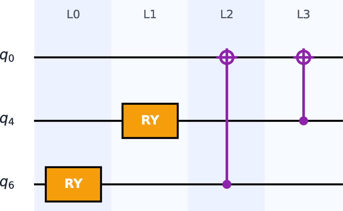
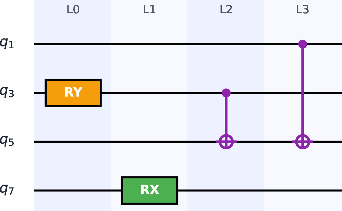
Figure 2: Critical-structure analysis. (a,b) Tier 1 circuits collapse to 2-gate minimal forms. (c,d) Tier 2 yields two structurally distinct circuits targeting orthogonal degenerate eigenstates of
CH2.. a — BeH2, b — LiH, c — Structure A, d — Structure B
width = 0.85, colspec = Q[40]Q[130]Q[30]Q[80]Q[80]Q[80]Q[60], cells = c, hline1,2,4,7 = -0.15em, Tier & System & \(n_q\) & Error
(mHa) & \(\bar{S}_{\mathrm{exact}}\) & \(\bar{S}_{\mathrm{circuit}}\) & \(\mathrm{MAE}_S\)
T1 & BeH2 STO-3G & 6 & 0.55 & 0.006 & 0.000 & 0.006
T1 & LiH (equil.) & 6 & 1.05 & 0.012 & 0.000 & 0.012
T3 & H2 (\(R\)=2.5 Å) & 4 & 0.00 & 0.974 & 0.974 & 0.000
T3 & H2O & 8 & 4.61 & 0.187 & 0.157 & 0.028
T3 & H4 Chain & 8 & 33.55 & 0.198 & 0.130 & 0.068
5.0.0.3 Tier 3: Representation.
Tier 3 evaluates whether QAS methods can represent strongly correlated ground states. A clear transition is observed: RL-based methods achieve near-exact solutions on H2_Stretch, while all methods fail to reach chemical accuracy on the
larger instances H2O_StrongCorr and H4_Chain.
Per-qubit entropy analysis (Table ¿tbl:tab:entropy95consistency?) sharpens this picture. On H2_Stretch, despite near-maximal ground-state entanglement (\(\bar{S}_{\mathrm{exact}} = 0.974\)),
pruned circuits achieve \(\mathrm{MAE}_S = 0.000\), confirming that methods are not biased toward product states and can faithfully encode strong correlation when the Hilbert space is small. On H2O_StrongCorr,
even when energy has not fully converged (\(\varepsilon \approx 4.6\) mHa), pruned circuits capture the dominant entanglement on \(q_2\)–\(q_7\) (\(\mathrm{MAE}_S = 0.028\)) while missing the weaker correlations on \(q_0\) and \(q_1\), suggesting that structural failure precedes energy failure. On
H4_Chain under all-to-all connectivity, \(\mathrm{MAE}_S = 0.068\) with boundary qubits \(q_1\) and \(q_6\) showing zero captured entanglement,
confirming that representation failure is structural rather than parametric. The effect of linear connectivity on H4_Chain is analyzed in Appendix 13.3, where \(\mathrm{MAE}_S\) rises to 0.121 and four boundary qubits lose all captured entanglement—demonstrating that energy and entanglement structure can decouple under connectivity constraints.
5.0.0.4 Tier 4: Topology.
Tier 4 evaluates whether QAS methods can realize required correlations under hardware connectivity constraints. On H3_Linear (2-fold degenerate, \(\mathrm{Gap}=0\)), enforcing nearest-neighbour connectivity
causes a clear performance drop relative to all-to-all, with errors increasing by more than an order of magnitude across methods. As the ground-state degeneracy of H3_Linear introduces the same eigenstate ambiguity as Tier 2, \(\mathrm{MAE}_S\) analysis is not directly applicable; the connectivity effect on entanglement structure is instead isolated on H4_Chain (Appendix 13.3). Training-stage
critical-structure analysis on H3_Linear reveals the mechanism: under all-to-all connectivity, retained circuits include long-range CNOTs enabling end-to-end information flow, while under linear connectivity, circuits reuse only short-range
local interactions, forming local hubs but failing to propagate correlations across the full system. The performance gap is thus not due to optimization failure but to a structural limitation in information routing.
5.0.0.5 Tier 5: Same-family scalability.
Tier 5 evaluates scalability under increasing system size with controlled molecular structure. On the BeH2 basis ladder (8–14 qubits), ground-state entanglement remains uniformly low (\(S_{\mathrm{max}} \le
0.039\)) and the spectrum remains gapped throughout, confirming that Hamiltonian complexity is controlled. Despite this, a sharp performance transition is observed: at 10 qubits, RL-based methods achieve high success rates (HyRLQAS 100%, CRLQAS 90%) with compact circuits (HyRLQAS mean 1.0 CNOT), while all other paradigms largely fail; at 12 and 14 qubits, all methods deteriorate to
near-zero evaluation success. Per-qubit entropy analysis confirms that the difficulty is not entanglement complexity: at 12 qubits, training circuits faithfully reproduce the exact ground-state entanglement (\(\mathrm{MAE}_S =
0.005\)) yet fail to stabilize, and at 14 qubits, even a structurally sound training circuit cannot be re-optimized reliably—the optimizer itself fails in the \(2^{14}\)-dimensional parameter space. Tier 5 thus
reveals two compounding scalability bottlenecks: search policy instability and parameter optimization failure, both independent of Hamiltonian correlation structure. Full results are provided in Appendix 13.4.
6 Conclusion↩︎
We introduced HamQASBench, which organizes evaluation around Hamiltonian structural fingerprints rather than molecular identity, and complements energy-based metrics with post-hoc critical-structure extraction and per-qubit entanglement analysis. Across five tiers spanning eleven molecules and up to 14 qubits, we find that energy accuracy is an unreliable proxy for structural correctness: methods can achieve chemical accuracy via over-parameterized circuits, commit to orthogonal eigenstates under degeneracy, or encode worse entanglement structure while reaching lower energy under connectivity constraints—failure modes that remain invisible to conventional evaluation. We hope HamQASBench provides a principled foundation for diagnosing and improving QAS methods beyond energy metrics alone.
6.0.0.1 Limitations.
First, the per-qubit entropy analysis (\(\mathrm{MAE}_S\)) is based on CRLQAS training-stage circuits, as it produces the largest pool of chemical-accuracy snapshots suitable for pruning.
While this provides a principled structural baseline, extending the analysis to other paradigms remains a direction for future work. Second, the ground-state degeneracy of H3_Linear introduces eigenstate ambiguity that precludes direct \(\mathrm{MAE}_S\) comparison; we address this by isolating the connectivity effect on entanglement structure using H4_Chain (Appendix 13.3), where degeneracy is absent.
7 Method Implementation Details↩︎
For fair comparison, all methods operate over a unified gate basis \(\{\mathrm{RX}, \mathrm{RY}, \mathrm{RZ}, \mathrm{CNOT}\}\) and a shared depth budget \(D\). Candidate circuits are allowed to terminate before \(D\) through
7.0.0.1 CRLQAS [9].
CRLQAS formulates QAS as a Markov decision process in which a DQN [42] agent sequentially inserts gates into a growing circuit. The step reward is defined as \[r_t = \begin{cases} +5 & \text{if } E_t < \xi_t \\ -5 & \text{if } t = L-1 \text{ and } E_t \geq \xi_t \\ \mathrm{clip}\!\left(\dfrac{E_{t-1} - E_t}{|E_{t-1} - E_{\min}| + \epsilon},\,-1,\,1\right) & \text{otherwise,} \end{cases}\] where \(\xi_t\) is an acceptance threshold that is either progressively tightened via a moving curriculum or held fixed, depending on the task. The policy is trained with \(n\)-step DQN (\(n=6\)) and an experience replay buffer. Episodes terminate upon reaching the acceptance threshold or the maximum depth \(D\). The gate set matches the benchmark standard with no adaptation required.
7.0.0.2 HyRLQAS [10].
HyRLQAS extends discrete-action QAS by predicting initial rotation angles alongside gate placement, providing warm-start initializations for the external optimizer rather than replacing it. A refinement mechanism further updates previously assigned angles after each gate insertion. The policy is trained with REINFORCE [43]. The gate set requires no adaptation. Episodes terminate upon reaching the acceptance threshold or maximum depth \(D\),following the same curriculum structure as CRLQAS.
7.0.0.3 QuantumDARTS [12].
QuantumDARTS maintains continuous architecture weights over \(\{\mathrm{Rz\text{-}Ry\text{-}Rz}, I, \mathrm{CNOT}\}\) and optimizes them jointly with gate parameters via Gumbel-softmax relaxation. Architecture weights are updated only during the search phase; after discretization, the exported circuit undergoes fixed-structure parameter re-optimization using the shared local optimizer. The search and evaluation spaces differ by design: identity slots allow circuits to terminate before \(D\), and each \(\mathrm{Rz\text{-}Ry\text{-}Rz}\) block is lowered to primitive \(\{\mathrm{RZ}, \mathrm{RY}, \mathrm{RZ}\}\) at evaluation time.
7.0.0.4 TFQAS [18].
TFQAS applies a three-stage progressive filtering pipeline. Stage 1 ranks \(S\) sampled circuits by DAG path count [44]; Stage 2 re-scores the top-\(R\) by expressibility [45]; Stage 3 applies the shared local optimizer to the top-\(K\) circuits. Gate count is sampled uniformly from \([1, D]\), enabling natural early termination. The original entangler set \(\{\mathrm{XX}, \mathrm{YY}, \mathrm{ZZ}\}\) is replaced with CNOT at search time.
7.0.0.5 GQEQAS [11].
GQEQAS trains an autoregressive transformer online: at each epoch it generates circuits, evaluates them via VQE, and updates with an energy-weighted gradient. Sequence length is sampled uniformly up to the depth budget, allowing early termination. Final energies are reported after parameter re-optimization using the shared local optimizer. The original operator pool is replaced with a discretized token pool over \(\{\mathrm{RX}, \mathrm{RY}, \mathrm{RZ}, \mathrm{CNOT}\}\).
8 Optimizer Parallelization and Execution Backend↩︎
8.0.0.1 Motivation.
Circuit-level parameter optimization is the primary computational bottleneck in HamQASBench. For a fixed circuit structure, an external optimizer must repeatedly query the circuit energy until convergence, and as qubit count increases each energy query becomes substantially more expensive. GPU-based state-vector simulation can accelerate individual queries, but its benefit is limited when the optimizer issues strictly sequential calls. Our design therefore targets optimizer structures that admit grouped evaluation and make better use of GPU throughput.
8.0.0.2 Rotosolve as the scalable optimizer.
Rotosolve is well matched to this setting. Each sweep over the active rotation parameters evaluates a fixed three-point probe set \(\{0, \pi/2, \pi\}\) per parameter and updates it analytically. With
rotosolve_sweeps\(=2\), two complete sweeps are performed per optimization call. Because all probe angles within a sweep are known in advance, the corresponding energy queries are assembled into a single
batched evaluation rather than launched sequentially. This exposes two levels of parallelism: probe circuits within a sweep are evaluated together via a batched state-vector backend, and \(k=10\) optimization environments
are overlapped across CUDA streams. COBYLA, by contrast, issues adaptive sequential queries (maximum global_iters\(=100\) iterations) and exposes little coarse-grained parallelism, which is why it is retained
only for small systems (\(\le 6\) qubits) where runtime remains manageable.
8.0.0.3 Empirical efficiency.
Table ¿tbl:tab:optimizer95speedup? reports wall-clock time per training episode on the BeH2 basis-set ladder using a representative CRLQAS workload. GPU\(^*\)
Rotosolve with \(k=10\) parallel environments reduces per-episode cost to 14.7–27.0 seconds across the 8q–14q range, compared to 195.7–338.0 seconds for CPU Rotosolve, enabling practical benchmarking at scales that would
otherwise be infeasible.
width = , colspec = Q[55]Q[75]Q[55]Q[55]Q[55]Q[55], cells = c, hline1,2,14 = -0.15em, hline6,10 = -dashed, 0.05em, Hardware &
Optimizer & 8q & 10q & 12q & 14q
CPU & COBYLA & 48.9 & 146.7 & 270.9 & 429.9
& Rotosolve & 42.7 & 144.9 & 195.7 & 338.0
& AdamSPSA & 69.7 & 218.4 & 439.1 & 934.2
& PSRAdam & 54.5 & 206.4 & 243.4 & 443.0
GPU & COBYLA & — & — & — & —
& Rotosolve & 19.0 & 16.2 & 21.1 & 63.2
& AdamSPSA & 95.6 & 98.3 & 110.9 & 218.8
& PSRAdam & 45.2 & 55.8 & 69.2 & 131.1
GPU\(^*\) & COBYLA & — & — & — & —
& Rotosolve & 14.7 & 12.9 & 13.4 & 27.0
& AdamSPSA & 79.0 & 70.7 & 81.3 & 104.2
& PSRAdam & 40.9 & 48.7 & 48.4 & 69.8
9 Training Hyperparameters and Compute Budget↩︎
9.0.0.1 Per-method training configuration.
Table ¿tbl:tab:hyperparams? lists the key hyperparameters for each method. For RL methods (CRLQAS, HyRLQAS), one episode denotes a complete circuit-construction trajectory of
at most \(D\) gate insertions, with 8 environments rolled out in parallel. The two methods share the same overall configuration except for batch size: CRLQAS uses a larger replay buffer update
(batch size 1000) while HyRLQAS uses batch size 16 consistent with its REINFORCE update rule. Both use 8000 episodes for simpler molecules and 15000 for larger or more challenging instances. For QuantumDARTS, the search phase runs for \(n_\mathrm{epochs}\) with \(n_\mathrm{inner}=10\) gradient steps per epoch; architecture weights are updated only during
this search phase, after which the best discrete circuit undergoes fixed-structure parameter re-optimization with COBYLA or Rotosolve. The configured post-search budget and learning rates vary by problem size as shown in
Table ¿tbl:tab:hyperparams?, but architecture parameters are not updated post-search. For TFQAS, no gradient updates are performed; the budget is expressed as the number of candidate circuits sampled. For
GQEQAS, one epoch draws online_sample_count\(=250\) circuits from the current generative model, evaluates them via VQE, and updates the transformer with the resulting
energy-weighted objective; 1000 epochs are used for simpler molecules and 1500 for larger instances.
width = , colspec = Q[70]Q[110]Q[70]Q[30]Q[250]Q[30], cells = c, hline1,2,7 = -0.15em, Method & Training unit & Budget & Depth \(D\) & Policy update & Batch size
CRLQAS & episode (\(\times\)8 envs) & 8k / 15k ep & 10 / 50 & DQN (\(n\)-step, \(n\!=\!6\)) & 1000
HyRLQAS & episode (\(\times\)8 envs) & 8k / 15k ep & 10 / 50 & REINFORCE & 16
QuantumDARTS & epoch (\(n_\mathrm{inner}\!=\!10\)) & 500–900 ep & 10 / 50 & Adam (\(\theta\): \(10^{-2}\)–\(5\!\times\!10^{-3}\), \(\alpha\): \(5\!\times\!10^{-3}\)–\(3\!\times\!10^{-3}\)) & —
TFQAS & candidate circuits & \(S\!=\!11\)k–\(23\)k & 10 / 50 & None & —
GQEQAS & epoch (online refresh) & 1k / 1.5k ep & 10 / 50 & Adam & —
9.0.0.2 Evaluation during training.
For all learning-based methods, periodic evaluation is performed every \(e_\mathrm{eval}\) episodes by sampling \(K_\mathrm{eval}=50\) circuits from the current model without gradient updates. The best circuit found across all evaluation checkpoints—measured jointly by energy error and CNOT count—is retained as the method’s final result. For TFQAS, evaluation is applied once after the top-\(K=50\) circuits undergo final VQE parameter optimization.
9.0.0.3 Training budget alignment.
Comparing training budgets across paradigms is non-trivial because one episode incurs fundamentally different computational costs depending on the method: an RL episode involves \(D\) sequential VQE calls during trajectory rollout, whereas one QuantumDARTS epoch processes all circuit slots simultaneously via a single backward pass. We adopt episode/epoch count as the primary budget axis and report wall-clock time per episode in Appendix 8 to allow cost-adjusted comparisons.
10 Molecule Generation and Hamiltonian Construction↩︎
Table ¿tbl:tab:mol95generation? lists the generation parameters for all molecules in HamQASBench. For each instance, we provide the molecular geometry, basis set, active space configuration (CAS), and the resulting number of qubits. All geometries are specified in Angstrom (Å). Electronic structure calculations use a singlet reference (\(\mathrm{mult}=1\)) unless otherwise noted. Frozen electrons are defined as the difference between the total and active electrons.
10.0.0.1 Implementation details.
Hamiltonians are generated using a standard quantum chemistry pipeline. We first perform mean-field calculations to obtain molecular orbitals, followed by active-space selection to define the CAS\((n_e, n_o)\) configuration. The resulting fermionic Hamiltonian is mapped to qubits via the Jordan–Wigner transformation. All instances use consistent numerical settings and deterministic workflows.
10.0.0.2 Reproducibility.
All Hamiltonians can be deterministically reconstructed from the parameters in Table ¿tbl:tab:mol95generation?, with no stochastic procedures involved, and are directly compatible with standard libraries such as PennyLane.
colspec = Q[15]Q[120]Q[240]Q[30]Q[70]Q[70]Q[70]Q[30], cells = c, hline1,2,13 = -0.15em, Tier & Molecule & Geometry (Å) & Charge & Basis & CAS\((n_e, n_o)\) & Frozen \(e^-\) & \(n_q\)
1 & BeH2_STO3G & Be(0,0,0); H(0,0,1.326); H(0,0,-1.326) & 0 & STO-3G & (2e, 3o) & 4 & 6
1 & LiH_Equil & Li(0,0,0); H(0,0,1.595) & 0 & STO-3G & (2e, 3o) & 2 & 6
2 & CH2 & C(0,0,0); H(0,0.86,0.73); H(0,-0.86,0.73) & 0 & STO-3G & (2e, 4o) & 6 & 8
3 & H2_Stretch & H(0,0,0); H(0,0,2.500) & 0 & STO-3G & (2e, 2o) & 0 & 4
3 & H2O_StrongCorr & O(0,0,0); H(0,1.186,0.918); H(0,-1.186,0.918) & 0 & STO-3G & (4e, 4o) & 6 & 8
3 & H4_Chain & H(0,0,0); H(0,0,1); H(0,0,2); H(0,0,3) & 0 & STO-3G & (4e, 4o) & 0 & 8
4 & H3_Linear\(^\ddag\) & H(0,0,0); H(0,0,1); H(0,0,2) & 1 & STO-3G & (2e, 3o) & 0 & 6
5 & BeH2_631G & Be(0,0,0); H(0,0,1.326); H(0,0,-1.326) & 0 & 6-31G & (2e, 4o) & 4 & 8
5 & BeH2_6311G & Be(0,0,0); H(0,0,1.326); H(0,0,-1.326) & 0 & 6-311G & (2e, 5o) & 4 & 10
5 & BeH2_CCPVDZ & Be(0,0,0); H(0,0,1.326); H(0,0,-1.326) & 0 & cc-pVDZ & (2e, 6o) & 4 & 12
5 & BeH2_CCPVDZ & Be(0,0,0); H(0,0,1.326); H(0,0,-1.326) & 0 & cc-pVDZ & (4e, 7o) & 2 & 14
\(\ddag\) H\(_3^+\) cation; Tier 4 uses nearest-neighbour connectivity.
11 Hamiltonian Fingerprint Theory↩︎
The field of quantum chemistry has historically analysed structural properties and, in particular, approximate solutions of the full configuration interaction (FCI) Hamiltonian to diagnose the complexity of the system. The structure of the FCI Hamiltonian exhibits, in overwhelming number of cases, sparsity with known couplings by excitation rank; high symmetry based on well established spin multiplicity and spatial group theory concepts; and diagonal dominance due to large contributions from mean-field terms compared to off-diagonal coupling. This has allowed the proliferation of classically computationally efficient methods that work in the majority of cases such as coupled cluster theory or truncated configuration interaction. Similarly, it has led to problem specific ansatz design for VQE on these problems such as the UCCSD ansatz used in the initial formulation of VQE. In particular, many existing theories and ansatz work well for problems described well by a single-reference Slater determinant which allows them to centre around the Hartree-Fock solution and its excitations.
However, it is well known that these theories and assumptions break down for larger, strongly correlated materials that we wish to study such as: open-shell systems, bond breaking, transition-metal complexes, and large biological systems which often require multi-reference solutions with complicated entanglement structure. We therefore aim to treat the common assumptions on the CI Hamiltonian instead as metrics to characterise the difficulty of the electronic structure problem and identify useful Hamiltonians for use as benchmarking.
11.1 Operator and Computational basis Fingerprints↩︎
As an example, iterative diagonalisation procedures commonly rely on the Hamiltonian being diagonally dominant. Consider a Hamiltonian \(H\) with matrix elements \(h_{i,j}\). Diagonal dominance is defined as: \[|h_{i,i}| \ge \sum_{i\ne j} |h_{i,j}|.\]
This is well justified using Gershgorin’s circle theorem, illustrated in Figure 1b) in the main text, which says that every eigenvalue of \(H\) lies within at least one of the Gershgorin discs which are discs centered at \(h_{i,i}\) with radius \(\sum_{i\ne j} |h_{i,j}|\). When the matrix is diagonally dominant, the circles are narrow and may become disjoint. If a disc or set of discs become isolated, then they will contain as many eigenvalues as they have discs, with each eigenvalue well bounded around the corresponding matrix element. Overlapping discs reflect strong off-diagonal coupling in the computational basis and can indicate multi-reference character and cause simple ansatz and classically efficient methods to lose accuracy.
We propose three related metrics to measure how a given Hamiltonian violates this property. The first is a direct measure of overall diagonal dominance in the Pauli operator basis. The remaining two are defined in the matrix representation in the computational basis: assuming diagonal dominance has been violated overall, they measure the fraction of rows that remain diagonally dominant and the value of the weakest diagonally dominant row.
We will now derive the metrics based on the definition of diagonal dominance. We start with a Hamiltonian in the Pauli operator basis:
\[H = \sum_i c_i P_i ,\]
where \(P_i\) are Pauli strings and \(c_i\) are their coefficients, we can write the matrix elements as an expectation value: \[h_{i,j} = \left\langle i \right|H\left| j \right\rangle = \sum_k c_k \left\langle i \right|P_k\left| j \right\rangle.\]
Now, for diagonal entries, the only contributions will be from \(P_i\) that have \(I\) and \(Z\) qubit components which will contribute either \(1\) or \(-1\). We can therefore write: \[h_{i,i} = \sum_{k\in\{I,Z\}} c_k a_{i,k},\] where \(a_{i,k}\) is either \(1\) or \(-1\) and is determined by how many \(Z\) in the Pauli string coincide with a qubit with state \(1\) in \(\left| i \right\rangle\).
To consider strings with \(X\) and \(Y\), consider enumerating the state into \(n\) qubits i.e. \(\left| i \right\rangle = \left| q_0q_1\ldots q_b \ldots q_{n-1} \right\rangle\) with some index \(b\). A Pauli string, \(P_k\) that has any \(X\) or \(Y\) at some qubit index \(b\) will flip \(q_b\) from \(0\) to \(1\) or vice versa. This means that any qubit string containing \(X\) or \(Y\) will not contribute to the diagonal component.
For off-diagonals, strings containing only \(Z\) and \(I\) will not contribute as they cannot transform computational basis states. \(P_k\) with \(X\) and \(Y\) strings will only contribute when \(\left| i \right\rangle\) is related to \(\left| j \right\rangle\) by flipping the qubits with \(X\) or \(Y\) terms. Since a single Pauli string cannot create a superposition between computational basis states, it will only map one basis state to another basis state, so, for each row \(i\), for each Pauli \(P_k\), there will be only one non-zero \(j\). Therefore, we can immediately treat the sum over the row, since each Pauli will only contribute to one element in the row: \[\sum_j h_{i,j} = \sum_{k\in\{X,Y\}} c_k b_{i,k},\] where \(b_{i,k} \in \{1,-1,i,-i \}\). Overall, we have diagonal dominance forming the following chain of inequalities: \[| \sum_k c_k b_{i,k} | \le \sum_j |h_{i,j}| \le |h_{ii}| = |\sum_k c_k a_k| \le \sum_k |c_k|,\] where we have used the triangle inequality for the last step. Note that this upper bound works for all rows, where the original diagonal dominance condition was only for each row. While this statement is true and can be evaluated to determine diagonal dominance, we also investigate a stronger statement. We can form an upper bound for the off-diagonals using the triangle inequality: \[\sum_j|h_{i,j}| \le \sum_{k\in\{X,Y\}} |c_k|,\] which gives us a sufficient but not necessary condition for diagonal dominance: \[\sum_{k \not\in\{I,Z\}} |c_k| \le \sum_{k \in\{I,Z\}} |c_k|.\]
We want to define an overall metric that can be a proxy for how difficult it is to find the ground state. We can use the fraction of the Pauli coefficients that contribute to the diagonal as a ratio of overall contribution:
\[r_Z = \frac{\sum_{P_i \in Z\text{-only}} |c_i|}{\sum_i |c_i|},\]
where as \(r_Z > 0.5\), the more diagonally dominant the Hamiltonian will be. We note that this is a metric independent of row, distinct from our computational metrics \(G_1\) and \(G_2\) which measure the proportion of rows and the weakest diagonal dominance row respectively.
11.2 Multiqubit interaction metric↩︎
Similarly, we take inspiration from results in quantum computational complexity theory. In complexity theory, the k-local Hamiltonian problem is QMA-complete. k-local refers to each Pauli string in the Hamiltonian having at most "k" non-identity terms i.e. only acting on "k" qubits at a time. In particular, it is well known that 2-local Hamiltonians can have ground states with long range non-trivial quantum correlations, the typical example being a 2D antiferromagnetic Heisenberg model and, similarly, it is why we can achieve universal gate sets for quantum computing with only two-qubit entangling gates.
As a comparison, 1-local Hamiltonians are trivial to find the ground state and are in P regardless of the number of qubits. To that end, we define a metric to determine the weight of the entangling terms, which cause the problem to be QMA-complete. Similarly, this also measures how badly the ground state can be approximated by the trivial 1-local component of the Hamiltonian.
11.3 Energy Metrics↩︎
The energy gap is a common metric for measuring difficulty of finding a ground state and is tied to degeneracy. Firstly, many ground state theorems are only applicable to gapped Hamiltonians. Secondly, for this work, we consider an energy gap of zero as equivalent to having degenerate ground states. Typically in chemistry, for degenerate ground states such as triplet states, the energy gap will be defined to the next highest triplet state or something similar. Indeed, the degeneracy due to spin multiplicity and spatial symmetry is well known and can be readily predicted. For our Hamiltonians, it is possible to remove degeneracy by restricting the Hilbert space to a specific spin/charge/symmetry sector, however we use degeneracy to create gapless Hamiltonians to serve as a challenge for architecture search algorithms, which can demonstrate its scaling when tackling real world problems with degeneracy that cannot be predicted or removed.
11.4 Ground state Metrics↩︎
Measuring multipartite entanglement structure is highly non-trivial and multiple competing metrics exist. Fortunately, bipartite entanglement metrics are well understood and, therefore, we propose to use the Von Neumann Entropy from separating one qubit from the ground state for each qubit. While this metric requires access to the exact ground state, it is common in quantum chemistry to calculate similar information theoretic quantities using approximations of the ground state. For instance, for larger benchmarks, we can use the 1-RDM, 2-RDM, or even a Matrix Product State approximation of the ground state which are able to be calculated with classical computers.
12 Critical-Structure Extraction Details↩︎
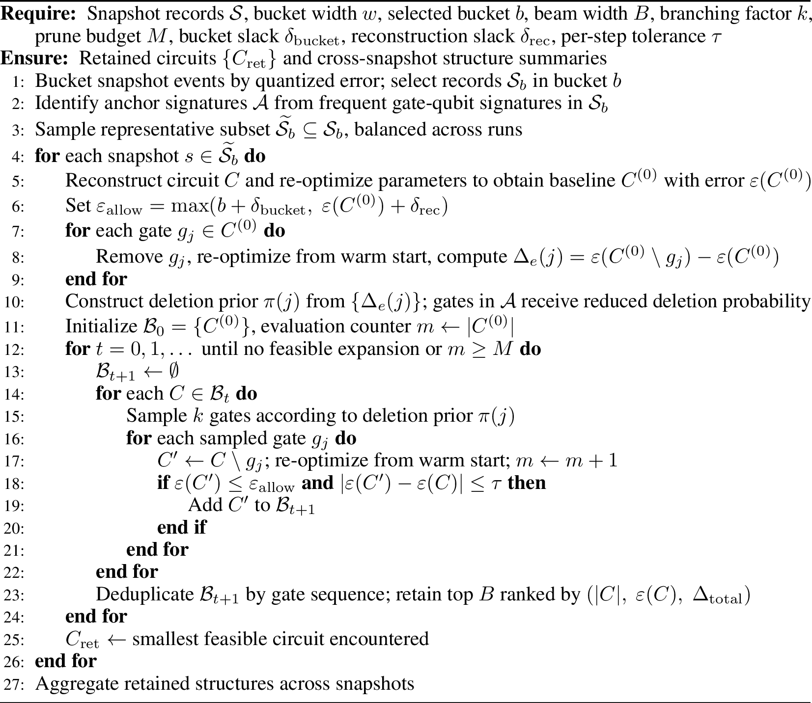
Algorithm 3 formalizes the critical-structure extraction procedure. Given low-error training snapshots from a fixed molecule–method setting, the procedure combines counterfactual gate ablation with constrained beam pruning under an explicit error budget, returning compact retained circuits and cross-snapshot structure summaries.
12.0.0.1 Snapshot collection and bucketing.
Snapshots \((C_i, \theta_i, \varepsilon_i)\) are grouped into quantized error buckets and analysis is restricted to a selected bucket, ensuring circuits are compared at a consistent performance level. Representative snapshots are sampled with bias toward late training and balanced across random seeds to avoid dominance by a single run.
12.0.0.2 Circuit reconstruction and baseline optimization.
Each snapshot is reconstructed into a gate-level circuit and parameters are re-optimized to obtain a stable baseline \(C^{(0)}\), accommodating minor discrepancies between stored traces and locally optimized circuits.
12.0.0.3 Counterfactual gate importance.
For each gate \(g_j \in C^{(0)}\), we remove it and re-optimize the remaining circuit from a warm start (inheriting current parameter values), computing \(\Delta_e(j) = \varepsilon(C^{(0)} \setminus g_j) - \varepsilon(C^{(0)})\). Using warm-start re-optimization ensures that \(\Delta_e(j)\) reflects the true structural contribution of \(g_j\) rather than a parameter initialization artifact.
12.0.0.4 Constrained beam pruning.
From the baseline importance scores, we construct a deletion prior \(\pi(j)\) inversely weighted by \(\Delta_e(j)\), so that gates with smaller degradation are more likely to be sampled for removal. Gates matching frequent gate-qubit signatures across snapshots (anchor gates) receive reduced deletion probability to protect structurally recurring motifs. At each pruning step, \(k\) gates are sampled per candidate according to \(\pi(j)\)—the prior is fixed from the baseline and not recomputed as the circuit shrinks. A candidate is retained only if it satisfies both the error tolerance \(\varepsilon_{\mathrm{allow}}\) and the per-step degradation bound \(\tau\). The beam retains the top \(B\) candidates ranked by gate count, energy error, and cumulative error degradation \(\Delta_{\mathrm{total}}\).
12.0.0.5 Outputs.
For each snapshot, the procedure returns the smallest retained circuit \(C_{\mathrm{ret}}\) and records its redundancy ratio \(\rho = (|C^{(0)}| - |C_{\mathrm{ret}}|) / |C^{(0)}|\). Across snapshots, retained gate-qubit signatures are aggregated to identify common structural motifs.
13 More Experiment Results↩︎
13.1 Training-stage Results and Eval Gap↩︎
Table ¿tbl:tab:main95results? reports the best circuits discovered during training for each method–molecule pair. Comparing against the evaluation-stage results in Table ¿tbl:tab:eval95results?, two patterns emerge.
First, for Tier 1 and the small-scale Tier 3 instance H2_Stretch, the training–eval gap is negligible: methods that find chemical-accuracy solutions during training reliably reproduce them at evaluation, indicating stable policy convergence
in simple and well-conditioned regimes.
Second, the gap widens substantially in more challenging settings. On T2_CH2, RL-based methods discover near-exact solutions during training (CRLQAS, HyRLQAS, GQEQAS all reach errors below \(10^{-6}\) mHa) but fail to reproduce them consistently at evaluation, reflecting the eigenstate commitment and policy instability described in Section 5. On Tier 3 larger instances and Tier 4, training-stage errors are systematically lower than eval-stage errors across all methods, suggesting that low-error circuits are discovered sporadically during exploration but do not
correspond to stable learned policies. TFQAS shows no training–eval gap by construction, as it is training-free and produces a single ranked set of candidates.
width = , colspec = Q[180]Q[120]Q[10]Q[10]Q[120]Q[10]Q[10]Q[120]Q[10]Q[10]Q[120]Q[10]Q[10]Q[120]Q[10]Q[10], cells = c, cell12 = c=30.157,
cell15 = c=30.161, cell18 = c=30.171, cell111 = c=30.165, cell114 =
c=30.167, cell82 = c=30.157, cell85 = c=30.161, cell88 = c=30.171,
cell811 = c=30.165, cell814 = c=30.167, hline1,2,8,9,15 = -0.15em, Molecule & T1_BeH2_6q (Shallow)
& & & T1_BeH2_6q (Depth) & & & T1_LiH_Equil_6q (Shallow) & & & T1_LiH_Equil_6q (Depth) & & & T2_CH2_8q & &
Method & Error & Cnot & Rot & Error & Cnot & Rot & Error & Cnot & Rot & Error & Cnot & Rot & Error & Cnot & Rot
CRLQAS & 2.68E-04 & 4 & 5 & 2.68E-04 & 5 & 4 & 6.03E-04 & 5 & 5 & 2.34E-04 & 18 & 10 & 6.19E-07 & 8 & 6
HyRLQAS & 5.54E-04 & 3 & 3 & 2.56E-04 & 21 & 11 & 1.05E-03 & 0 & 5 & 2.47E-04 & 12 & 7 & 6.19E-07 & 11 & 5
QuantumDARTS & 5.54E-04 & 11 & 6 & 6.69E-05 & 90 & 48 & 1.05E-03 & 3 & 3 & 1.05E-03 & 3 & 3 & 5.66E-03 & 66 & 22
GQEQAS & 5.54E-04 & 0 & 2 & 5.54E-04 & 0 & 3 & 1.05E-03 & 8 & 8 & 1.05E-03 & 4 & 19 & 6.20E-07 & 10 & 17
TFQAS & 5.54E-04 & 5 & 4 & 1.89E-02 & 26 & 23 & 1.05E-03 & 5 & 4 & 1.01E-02 & 24 & 21 & 3.69E-01 & 35 & 26
Molecule & T3_H2_Stretch_4q & & & T3_H2O_StrongCorr_8q & & & T3_H4_Chain_8q & & & T4_H3_Linear_6q_All & & & T4_H3_Linear_6q_Linear & &
Method & Error & Cnot & Rot & Error & Cnot & Rot & Error & Cnot & Rot & Error & Cnot & Rot & Error & Cnot & Rot
CRLQAS & 4.44E-11 & 8 & 4 & 5.87E-03 & 34 & 25 & 3.38E-02 & 39 & 12 & 1.36E-03 & 25 & 19 & 1.69E-02 & 26 & 19
HyRLQAS & 1.41E-07 & 13 & 7 & 6.46E-03 & 26 & 12 & 3.98E-02 & 16 & 11 & 9.36E-03 & 27 & 11 & 2.35E-02 & 9 & 7
QuantumDARTS & 2.44E-03 & 24 & 12 & 1.43E-01 & 13 & 6 & 6.78E-02 & 13 & 9 & 4.64E-02 & 44 & 9 & 4.64E-02 & 19 & 6
GQEQAS & 4.39E-05 & 4 & 12 & 4.67E-02 & 0 & 6 & 6.69E-02 & 7 & 24 & 2.35E-02 & 7 & 8 & 4.64E-02 & 3 & 12
TFQAS & 4.71E-03 & 28 & 19 & 2.91E-01 & 37 & 32 & 7.80E-01 & 40 & 29 & 1.71E-01 & 24 & 24 & 2.17E-01 & 24 & 24
13.2 Tier 1 Full Gate Statistics↩︎
Table ¿tbl:tab:tier195full? reports the complete gate statistics for all chemical-accuracy circuits discovered during training in Tier 1, covering both BeH2_STO3G and LiH_Equil across all methods and budget
settings. Across both molecules, HyRLQAS consistently achieves the lowest redundancy rates (6.7% shallow and 25.3% deep on BeH2_STO3G; 34.9% on LiH_Equil), indicating that its hybrid action space
effectively suppresses unnecessary gate placement even when a larger budget is available. All other methods show substantially higher redundancy, with QuantumDARTS exceeding 92% across all settings.
width = , colspec = Q[180]Q[120]Q[10]Q[10]Q[120]Q[10]Q[10]Q[120]Q[10]Q[10]Q[120]Q[10]Q[10]Q[120]Q[10]Q[10], cells = c, cell12 = c=30.157,
cell15 = c=30.161, cell18 = c=30.171, cell111 = c=30.165, cell114 =
c=30.167, hline1,2,8 = -0.15em, Molecule & T5_BeH2_6q & & & T5_BeH2_631G_8q & & & T5_BeH2_6311G_10q & & & T5_BeH2_CCPVDZ_12q & & &
T5_BeH2_CCPVDZ_14q & &
Method & Error & Cnot & Rot & Error & Cnot & Rot & Error & Cnot & Rot & Error & Cnot & Rot & Error & Cnot & Rot
CRLQAS & 2.68E-04 & 4 & 5 & 1.15E-04 & 42 & 10 & 2.48E-04 & 35 & 10 & 1.24E-03 & 46 & 17 & 5.01E-03 & 18 & 9
HyRLQAS & 5.54E-04 & 3 & 3 & 2.34E-04 & 18 & 9 & 2.48E-04 & 13 & 6 & 1.24E-03 & 42 & 32 & 5.68E-03 & 33 & 6
QuantumDARTS & 5.54E-04 & 11 & 6 & 2.17E-03 & 1 & 6 & 8.97E-04 & 1 & 6 & 2.60E-01 & 19 & 3 & 3.01E-01 & 114 & 12
GQEQAS & 5.54E-04 & 0 & 2 & 2.17E-03 & 7 & 21 & 8.96E-04 & 6 & 12 & 1.87E-03 & 8 & 11 & 6.15E-03 & 0 & 9
TFQAS & 5.54E-04 & 5 & 4 & 2.07E-01 & 36 & 31 & 3.83E-01 & 51 & 41 & 1.45E-01 & 50 & 29 & 3.26E-01 & 45 & 32
BeH2 STO-3G
width = , colspec = Q[120]Q[80]Q[60]Q[60]Q[70]Q[70]Q[80]Q[80], cells = c, hline1,2,7,12 = -0.15em, Method & Budget & Rot mean & Rot std & CNOT mean &
CNOT std & Total mean & Redundancy
CRLQAS & shallow & 3.17 & 1.22 & 2.72 & 1.77 & 5.89 & 66.1%
HyRLQAS & shallow & 2.06 & 0.39 & 0.08 & 0.52 & 2.14 & 6.7%
GQEQAS & shallow & 7.78 & 1.70 & 0.14 & 0.34 & 7.92 & 74.7%
TFQAS & shallow & 4.39 & 0.70 & 5.45 & 0.62 & 9.85 & 79.7%
QuantumDARTS & shallow & 9.60 & 3.10 & 29.20 & 17.38 & 38.80 & 94.8%
CRLQAS & deep & 4.45 & 3.17 & 5.65 & 6.00 & 10.10 & 80.2%
HyRLQAS & deep & 2.21 & 1.08 & 0.47 & 2.45 & 2.68 & 25.3%
GQEQAS & deep & 11.79 & 4.54 & 1.75 & 3.48 & 13.54 & 85.2%
TFQAS & deep & — & — & — & — & — & —
QuantumDARTS & deep & 9.60 & 3.84 & 22.75 & 13.88 & 32.35 & 93.8%
LiH (equil.)
width = , colspec = Q[120]Q[80]Q[60]Q[60]Q[70]Q[70]Q[80]Q[80], cells = c, hline1,2,11 = -0.15em, Method & Budget & Rot mean & Rot std & CNOT mean & CNOT
std & Total mean & Redundancy
CRLQAS & shallow & 3.06 & 1.22 & 2.88 & 1.76 & 5.94 & 66.3%
HyRLQAS & shallow & 2.02 & 0.36 & 0.11 & 0.59 & 2.13 & 6.1%
GQEQAS & shallow & 7.44 & 2.47 & 0.07 & 0.37 & 7.51 & 73.4%
TFQAS & shallow & 4.11 & 0.70 & 5.48 & 0.58 & 9.59 & 79.2%
CRLQAS & deep & 4.97 & 3.69 & 6.47 & 6.73 & 11.43 & 82.5%
HyRLQAS & deep & 2.34 & 1.46 & 0.73 & 3.16 & 3.07 & 34.9%
QuantumDARTS & deep & 8.80 & 3.96 & 16.70 & 14.99 & 25.50 & 92.2%
GQEQAS & deep & 9.81 & 6.37 & 6.36 & 7.43 & 16.17 & 87.6%
TFQAS & deep & — & — & — & — & — & —
13.3 Topology Analysis: H4Chain Connectivity Comparison↩︎
To isolate the effect of connectivity constraints on entanglement structure encoding—independent of the eigenstate ambiguity present in the degenerate H3_Linear instance—we apply per-qubit entropy analysis to H4_Chain under two
connectivity settings: all-to-all and nearest-neighbour linear.
colspec = Q[100]Q[80]Q[80]Q[80]Q[60], cells = c, hline1,2,4 = -0.15em, Connectivity & Error (mHa) & \(\bar{S}_{\mathrm{exact}}\)
& \(\bar{S}_{\mathrm{circuit}}\) & \(\mathrm{MAE}_S\)
All-to-all & 33.55 & 0.198 & 0.130 & 0.068
Linear & 48.03 & 0.198 & 0.077 & 0.121
Table ¿tbl:tab:h495connectivity? shows that enforcing linear connectivity increases \(\mathrm{MAE}_S\) from 0.068 to 0.121 while also worsening energy error from 33.55 to 48.03 mHa. The per-qubit breakdown in Table ¿tbl:tab:h495perqubit? reveals the structural mechanism underlying this degradation.
colspec = Q[100]Q[40]Q[40]Q[40]Q[40]Q[40]Q[40]Q[40]Q[40], cells = c, hline1,2,5 = -0.15em, & \(q_0\) & \(q_1\) & \(q_2\) & \(q_3\) & \(q_4\) & \(q_5\) & \(q_6\) & \(q_7\)
Exact & .124 & .124 & .274 & .274 & .284 & .284 & .109 & .109
All-to-all & .062 & .000 & .213 & .245 & .245 & .213 & .000 & .062
Linear & .000 & .000 & .153 & .153 & .153 & .153 & .000 & .000
Under all-to-all connectivity, the pruned circuit captures interior qubit entanglement (\(q_2\)–\(q_5\)) reasonably well but fails on boundary qubits \(q_1\) and \(q_6\) (circuit \(S = 0\) vs.exact \(\approx 0.12\)). Under linear connectivity, this failure extends to all four boundary qubits (\(q_0, q_1, q_6, q_7\)), with \(\bar{S}_{\mathrm{circuit}}\) dropping from 0.130 to 0.077. Critically, the linear-connectivity circuit achieves higher energy error despite encoding less entanglement structure, confirming the decoupling between energy and structural fidelity identified in Section 5: a circuit can find a lower-energy solution in a restricted topology by concentrating gates on interior qubits, while systematically failing to represent the boundary correlations required by the Hamiltonian. This demonstrates that connectivity constraints impose a structural bottleneck that energy metrics alone cannot detect.
13.4 Tier 5 Full Scalability Results↩︎
Table ¿tbl:tab:tier595full? reports training-stage and evaluation-stage results for all methods across the BeH2 basis ladder. Three observations sharpen the main-text analysis.
13.4.0.1 10-qubit as the key inflection point.
At 10 qubits (BeH2_6311G), methods stratify into three tiers: HyRLQAS achieves 100% evaluation success rate with a mean of 1.0 CNOT per chemical-accuracy circuit, CRLQAS achieves
90% with a mean of 4.5 CNOTs, QuantumDARTS succeeds sporadically (15%), and GQEQAS and TFQAS fail entirely. The low CNOT counts for both RL methods confirm that
they correctly exploit the near-product ground-state structure (\(S_{\max} = 0.011\)) at this scale.
13.4.0.2 12-qubit: solutions exist but cannot stabilize.
At 12 qubits (BeH2_CCPVDZ), CRLQAS discovers circuits reaching 1.24 mHa during training (below chemical accuracy) with a training success rate of 0.1%, but evaluation success rate drops to 0%.
Critical-structure extraction confirms that 6 such circuits exist in the training trajectory; their gate counts range from 8 to 64 with redundancy rates of 25–78%, indicating that the policy remains in an exploratory regime and has not converged to a
compact reusable structure.
13.4.0.3 14-qubit: complete failure across all methods.
At 14 qubits, no method achieves chemical accuracy at either training or evaluation stage. CRLQAS produces the lowest evaluation error (6.15 mHa), still more than four times above the chemical accuracy threshold. The exponential growth of the search space (\(2^{14} = 16{,}384\) dimensions) appears to be the dominant bottleneck, consistent with the controlled entanglement structure across the ladder.
width = , colspec = Q[100]Q[80]Q[60]Q[60]Q[60]Q[60], cells = c, hline1,2,7,12,17,22 = -0.15em, Method & System & Train Best (mHa) & Train SR & Eval Best
(mHa) & Eval SR
CRLQAS & 8q & 1.99 & 0.0% & 0.23 & 0%
HyRLQAS & 8q & 0.23 & 0.1% & 2.17 & 0%
QuantumDARTS & 8q & — & — & 2.17 & 0%
GQEQAS & 8q & — & — & 24.57 & 0%
TFQAS & 8q & — & — & 197.39& 0%
CRLQAS & 10q & 0.13 & 90.2% & 0.90 & 90%
HyRLQAS & 10q & 0.90 & 98.7% & 0.90 & 100%
QuantumDARTS & 10q & — & — & 0.90 & 15%
GQEQAS & 10q & — & — & 35.48 & 0%
TFQAS & 10q & — & — & 390.42& 0%
CRLQAS & 12q & 1.24 & 0.1% & 2.00 & 0%
HyRLQAS & 12q & 2.00 & 0.0% & — & 0%
QuantumDARTS & 12q & — & — & 2.00 & 0%
GQEQAS & 12q & — & — & 269.68& 0%
TFQAS & 12q & — & — & 209.00& 0%
CRLQAS & 14q & 5.15 & 0.0% & 6.15 & 0%
HyRLQAS & 14q & 6.15 & 0.0% & — & 0%
QuantumDARTS & 14q & — & — & 273.00& 0%
GQEQAS & 14q & — & — & 711.00& 0%
TFQAS & 14q & — & — & 6.19 & 0%
13.4.0.4 Entanglement structure is not the bottleneck.
Per-qubit entropy analysis across the ladder confirms that ground-state entanglement complexity remains controlled throughout (Table ¿tbl:tab:tier595entropy?). At 10 qubits, solved circuits achieve \(\mathrm{MAE}_S = 0.001\). At 12 qubits, the 6 near-chemical-accuracy circuits discovered during training all reproduce the same entanglement profile (\(\mathrm{MAE}_S = 0.005\), Std \(= 0.000\)) despite gate counts ranging from 8 to 64—the policy has not converged to a compact structure, but when it does find a solution it correctly encodes the quantum state. At 14 qubits, a single training circuit (25 gates, 5.92 mHa) is available for analysis; its \(\mathrm{MAE}_S = 0.018\) confirms the ground state remains near-product (\(S_{\max} = 0.039\)). However, critical-structure extraction re-optimization recovers only 328 mHa from this circuit, compared to the training error of 5.92 mHa—the circuit structure is sound but the optimizer fails to recover the correct parameters in the \(2^{14} = 16{,}384\)-dimensional space within the allotted restarts. This reveals a two-layer failure at 14 qubits: the search policy can occasionally discover a structurally correct circuit, but neither the policy nor the optimizer can reliably exploit it. Together, these results confirm that performance degradation across the ladder is driven by search space growth rather than increasing entanglement complexity, directly supporting the Tier 5 design rationale.
colspec = Q[80]Q[30]Q[80]Q[80]Q[80]Q[80], cells = c, hline1,2,5 = -0.15em, System & \(n_q\) & Error (mHa) & \(\bar{S}_{\mathrm{exact}}\) & \(\bar{S}_{\mathrm{circuit}}\) & \(\mathrm{MAE}_S\)
BeH2 6-311G & 10 & 0.13 & 0.005 & 0.004 & 0.001
BeH2 cc-pVDZ & 12 & 1.24 & 0.011 & 0.006 & 0.005
BeH2 cc-pVDZ & 14 & 5.92\(^\dagger\) & 0.020 & 0.002 & 0.018
\(\dagger\) Training-stage error; critical-structure extraction reoptimization baseline = 328 mHa.