1 Introduction↩︎

Generative modeling has become a central topic in modern machine learning, driven by the remarkable progress of score-based generative models [1]–[3]. These models provide a flexible framework for learning complex high-dimensional distributions and generating realistic synthetic samples. Their success relies on gradually perturbing the data distribution through a forward noising process and then learning a reverse mechanism that transforms noise back into data. This paradigm has led to impressive empirical performance across a wide range of applications, including computer vision [4], [5], natural language processing [6], and other domains where realistic data generation is crucial. Inspired by Hamiltonian Monte Carlo, second-order variants such as critically-damped Langevin diffusions (CLDs) [7] have also been proposed as extensions of conventional diffusion models.

Beyond their empirical success, diffusion-based models have been extensively studied from a theoretical perspective, particularly through the lens of sampling error. This error is commonly decomposed into three components: mixing error, discretization error, and approximation error. Existing works establish sampling guarantees for SGMs [8]–[13] and CLDs [8], [11], [14]. Much of this literature focuses on the first two sources of error, often assuming that the approximation error is sufficiently small. However, the approximation error itself depends on both the statistical error induced by the chosen model class and the optimization error arising from the training procedure.

Several works have established generalization bounds for diffusion models [15]–[20]. In contrast, the optimization error arising from the training of these models remains comparatively less explored. Diffusion models are typically trained using denoising score matching [21]. In this direction, [22] analyze the approximation error of diffusion models trained by gradient descent through a Neural Tangent Kernel (NTK) analysis [23]. More recently, [24] studies the optimization dynamics of gradient descent for overparameterized score matching in the simplified setting of learning a single Gaussian distribution, using a gradient Expectation-Maximization algorithm. However, both works focus on gradient descent, whereas practical diffusion models are commonly trained using SGD and its variants [25], [26]. Moreover, [22] assumes bounded data, while [24] assumes that the target distribution is Gaussian; both assumptions are restrictive and do not capture the complexity of real-world data distributions.

In this work, we study the optimization error of score-based diffusion models trained with SGD. We first establish a non-asymptotic convergence rate for the expected squared gradient norm of score-based models under general score parameterizations, building on classical results from non-convex stochastic optimization. This result provides a general optimization guarantee for the denoising score-matching objective, but it does not directly control the score-approximation error. Moreover, the assumptions required for this guarantee restrict the admissible neural architectures and, in particular, exclude ReLU activation functions. To obtain direct approximation guarantees, we then analyze overparameterized two-layer ReLU networks trained with stochastic gradients. Using an NTK analysis, we derive non-asymptotic error bounds along the SGD trajectory for the denoising score-matching objective. Finally, we study the role of the reweighting factor, namely the prefactor multiplying the denoising score-matching loss, and quantify its effect on both optimization and sampling.

More precisely, our contributions are summarized as follows.

• We establish non-convex optimization guarantees for the weighted denoising score-matching objective under general score parameterizations. Our analysis shows that SGD converges at rate \(\mathcal{O}(\log n/\sqrt{n})\) in expected squared gradient norm, and explicitly captures the impact of mini-batches, stochastic gradient variance, and schedule-dependent loss weights.

• We provide an NTK analysis of overparameterized two-layer ReLU score networks specifically tailored to diffusion training. This leads to a non-asymptotic bound on the projected denoising score-matching loss along the SGD trajectory. Unlike prior works based on deterministic gradient descent, bounded data assumptions, or Gaussian target distributions, our framework directly handles stochastic optimization and allows for sub-Gaussian data distributions.

• Using our bounds, we analyze how the reweighting factor in the denoising score-matching loss affects both optimization and sampling. This provides theoretical guidance for its choice and offers an optimization-based explanation for weighting strategies that have proved effective in state-of-the-art diffusion models.

2 Notation and Background↩︎

2.1 Notation↩︎

Let \(\mathcal{P}(\mathbb{R}^d)\) denote the set of probability measures on \(\mathbb{R}^d\). We use \(\pi\) for probability measures and \(p\) for their densities with respect to the Lebesgue measure when they exist. The identity matrix of size \(d\) is written \(\mathbf{I}_d\). For \(x,y\in \mathbb{R}^d\), we denote by \(\langle x,y \rangle\) the standard inner product of \(\mathbb{R}^d\), by \(\|\cdot\|\) the Euclidean norm for vectors and its induced operator norm for matrices. Let \(\|\cdot\|_F\) be the Frobenius norm defined for \(A \in \mathbb{R}^{d \times d}\) as \(\|A \|_F :=\sqrt{\text{Tr} (A^\top A)}\). For random vectors \(X,Y \in \mathbb{R}^d\), define \(\|X\|_{L_2} := (\mathbb{E}[ \|X\|^2])^{1/2}\) and we write \(X \perp Y\) to mean that \(X\) is independent of \(Y\).

2.2 Score-based Generative Models↩︎

2.2.0.1 Forward noising process.

Let \(\pi_{\rm data}\in \mathcal{P}(\mathbb{R}^d)\) denote the target data distribution from which we wish to generate new samples. In generative machine learning, one does not observe \(\pi_{\rm data}\) directly. Instead, one has access to i.i.d. samples \(X_1^{\rm data},\dots,X_N^{\rm data}\sim \pi_{\rm data}\). SGMs construct a stochastic transport that progressively maps \(\pi_{\rm data}\) toward a simple reference distribution \(\pi_\infty\), and then approximately reverse this transport to generate new samples from the data law. In particular, they rely on a forward linear noising process defined as the solution to the following SDE: \[\label{eq:forward95sde} \mathrm{d}\overrightarrow X_t = - \alpha \beta_t \overrightarrow X_t \,\mathrm{d}t + \sqrt{2 \beta_t}\,\mathrm{d}B_t, \qquad X_0 \sim \pi_{\rm data} \,,\tag{1}\] where \((B_t)_{t \ge 0}\) is a standard Brownian motion in \(\mathbb{R}^d\), \(\beta_t : [0,T] \to \mathbb{R}_{\ge 0}\) is a time-dependent noise schedule, and \(\alpha \geq 0\). This linear SDE admits an explicit time marginal representation [13], for each fixed \(t \in [0,T]\): \[\label{eq:forward95marginal} \overrightarrow X_t \stackrel{\mathcal{L}}{=} m_t X_0 + \sigma_t Z \,, \qquad \text{where} \qquad Z \sim \mathcal{N}(0, \mathbf{I}_d) \,, \qquad Z \perp X_0 \,,\tag{2}\] with \(m_t := \exp (-\alpha \int_0^t \beta_s \,\mathrm{d}s)\) and \(\sigma_t^2 :=2 \int_0^t \beta_s \exp ( -2\alpha \int_s^t \beta_u \mathrm{d}u ) \mathrm{d}s\).

Equation 1 covers the standard forward diffusions used in the score-based modeling literature. When \(\alpha=0\), one has \(m_t\equiv 1\) and \(\sigma_t^2 = 2\int_0^t \beta_s\,\mathrm{d}s\); this corresponds to the variance-exploding (VE) regime used in score-based generative modeling [2], [27]. When \(\alpha=1\), the dynamics recover the usual variance-preserving (VP) family underlying diffusion probabilistic models [1], [3].

2.2.0.2 Backward process and generative model.

Under mild regularity assumptions [28], [29], the process defined in 1 admits a time-reversed process \((\overrightarrow X_t)_{t\in[0,T]} \stackrel{\mathcal{L}}{=} (\overleftarrow X_{T-t})_{t\in[0,T]}\) governed by \[\label{eq:backward95sde} \mathrm{d}\overleftarrow X_t = \Big( \alpha \beta_{T-t} \overleftarrow X_t + 2 \beta_{T-t} \nabla \log p_{T-t}(\overleftarrow X_t) \Big)\mathrm{d}t + \sqrt{2 \beta_{T-t}} \mathrm{d}B_t \,, \qquad \overleftarrow X_0 \sim p_T\tag{3}\] where \(p_t\) denotes the density of \(\overrightarrow X_t\). The reverse-time dynamics in 3 turn score estimation into a principled generative mechanism. Indeed, if one has access to the exact score \(\nabla \log p_t\) and could sample from the terminal law \(p_T\), then simulating the reverse process from \(\overleftarrow X_0\sim p_T\) would recover the data distribution exactly at time \(T\), i.e. \(\overleftarrow X_T\sim\pi_{\rm data}\). Modern SGMs can therefore be understood as approximate implementations of this ideal reverse-time sampler. Their accuracy is governed by three main sources of error: numerical discretization of the reverse SDE 3 , mismatch between the forward terminal law \(p_T\) and the reference distribution \(\pi_\infty\), and score learning error, namely the discrepancy between the learned score approximation and the true score function \((x,t) \to \nabla \log p_{T-t}(x)\) . The last term itself combines generalization error and optimization error.

2.2.0.3 Score matching.

To learn the score function, one introduces a parametric model \(s_\theta:\mathbb{R}^d\times[0,T]\to\mathbb{R}^d\), typically a deep neural network, and fits it by minimizing a time-averaged Fisher divergence \[\begin{align} \label{eq:score95matching} \mathcal{L}_{\rm SM}(\theta) &:= \frac{1}{2} \int_0^T \lambda(t)\, \mathbb{E}\left[ \|\mathsf{s}_\theta(\overrightarrow X_t,t)-\nabla \log p_t(\overrightarrow X_t)\|^2 \right] \mathrm{d}t \,, \end{align}\tag{4}\] where \(\lambda:[0,T]\to\mathbb{R}_{>0}\) is a weighting function. The difficulty with 4 is that the marginal score \(\nabla \log p_t\) is not available in closed form as it directly depends on \(\pi_{\rm data}\). That is why, most modern diffusion models are trained instead using conditional score matching \[\label{eq:csm} \mathcal{L}_{\rm DSM}(\theta) := \frac{1}{2} \int_0^T \lambda(t)\, \mathbb{E}\left[ \|\mathsf{s}_\theta(\overrightarrow X_t,t)-\nabla \log p_{t|0}(\overrightarrow X_t\mid X_0)\|^2 \right] \mathrm{d}t \,,\tag{5}\] where \(\nabla \log p_{t|0}(\overrightarrow X_t\mid X_0)\) is fully explicit as \(\overrightarrow X_t \mid X_0 \sim \mathcal{N} ( m_t X_0,\;\sigma_t^2 \mathbf{I}_d )\). Under standard square-integrability assumptions, since \(\nabla \log p_t(\overrightarrow X_t) = \mathbb{E}[\nabla \log p_{t|0}(\overrightarrow X_t \mid X_0)\mid \overrightarrow X_t],\) the Pythagorean identity for conditional expectation yields \[\mathbb{E}[ \|s_\theta(\overrightarrow X_t,t)-\nabla \log p_{t|0}(\overrightarrow X_t\mid X_0)\|^2 ] = \mathbb{E}\![ \|s_\theta(\overrightarrow X_t,t)-\nabla \log p_t(\overrightarrow X_t)\|^2 ] + C_t \,,\] where \(C_t\) does not depend on \(\theta\). Therefore, 4 and 5 have the same minimizers [21].

For stochastic optimization, it is convenient to rewrite the time integral in 5 as an expectation. Let \(q\) be a probability density on \((0,T]\), and let \(\tau\sim q\) be independent of \((X_0,Z)\). The choice of \(q\) does not change the population objective; it only specifies how time indices are sampled during training. Then \[\begin{align} \mathcal{L}_{\rm DSM}(\theta) &= \frac{1}{2}\, \mathbb{E}\!\left[ \frac{\lambda(\tau)}{q(\tau)} \|s_\theta(\overrightarrow X_\tau,\tau)-\nabla_x \log p_{\tau|0}(\overrightarrow X_\tau\mid X_0)\|^2 \right] \,. \label{eq:csm95expectation} \end{align}\tag{6}\] Since the conditional score is explicit for the Gaussian forward kernel, 6 is a fully tractable population objective.

3 Convergence Analysis for General Score Parameterizations↩︎

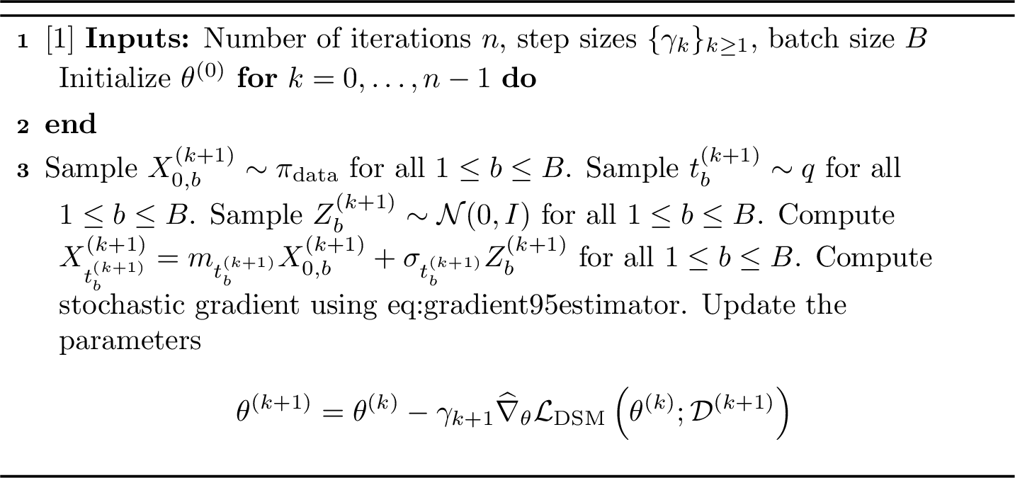
In this section, we derive convergence rates of SGD for the weighted denoising score-matching objective under general score parameterizations. SGD generates a sequence of parameter iterates as follows: let \(\theta^{(0)}\in\Theta\), and for all \(k\in\mathbb{N}\), \[\label{eq:SGD} \theta^{(k+1)} = \theta^{(k)} - \gamma_{k+1} \widehat{\nabla}_{\theta}\mathcal{L}_{\rm DSM} \left(\theta^{(k)};\mathcal{D}^{(k+1)}\right),\tag{7}\] where \(\{\gamma_k\}_{k\ge 1}\) is a sequence of positive step sizes and \(\widehat{\nabla}_{\theta}\mathcal{L}_{\rm DSM}(\theta^{(k)};\mathcal{D}^{(k+1)})\) is a stochastic estimator of the gradient computed from the mini-batch \[\mathcal{D}^{(k)}=\big\{(X^{(k)}_{0,b}, t^{(k)}_{b}, Z^{(k)}_{b})\big\}_{b=1}^B \,,\] with \(X^{(k)}_{0,b} \sim \pi_{\rm data}\), \(t^{(k)}_{b} \sim q\), and \(Z^{(k)}_{b} \sim \mathcal{N}(0,\mathbf{I}_d)\) independently for \(b=1,\dots,B\). The resulting stochastic gradient estimator is given by \[\label{eq:gradient95estimator} \widehat{\nabla}_{\theta}\mathcal{L}_{\rm DSM}(\theta^{(k)};\mathcal{D}^{(k+1)}) = \frac{1}{B}\sum_{b=1}^B g^{(k+1)}_{b} \,,\tag{8}\] where \(g^{(k+1)}_{b}\) denotes the stochastic gradient associated with a single sample, defined in 18 . The full procedure is detailed in Algorithm 2. We establish the convergence guarantees under the following regularity assumptions on the score network.

Assumption 1 imposes data-dependent Lipschitz and smoothness conditions on the score network, which are weaker than requiring uniform global bounds. Similar assumptions on the score function appear in the analysis of variational autoencoders [30] and policy-gradient methods [31]. In particular, [30] show that neural networks with bounded weights and standard smooth activations, such as sigmoid, tanh, and softplus, a smooth approximation to the ReLU, satisfy such conditions. However, Assumption 1 only controls the sensitivity of the network with respect to the parameters; it does not impose a uniform bound on the network output itself. This motivates the additional growth condition introduced next.

Assumption 2 controls the growth of the score network with respect to the input, requiring its magnitude to increase at most polynomially in \(\|x\|\). This is a natural stability condition: many theoretical analyses of score-based diffusion models impose regularity or growth assumptions on the true score, and in common settings such as Gaussian or log-concave targets the score has at most linear growth in \(\|x\|\) [12], [32], [33]. Together with Assumption 1, this condition ensures that the denoising score matching objective is smooth, which is essential for establishing non-asymptotic convergence guarantees for SGD.

Theorem 1 recovers the standard non-asymptotic \(\mathcal{O}(\log n/\sqrt n)\) convergence rate for nonconvex stochastic optimization, while making explicit the dependence on the mini-batch size, the stochastic gradient variance, and the time-dependent weighting of the denoising score-matching objective.

For a fixed time \(t\in[0,T]\), the bound in Theorem 1 with time reweighting scales as \(\lambda(t)/(\sigma_t^2 q(t))\), where \(\lambda(t)\) is the weighting function and \(q(t)\) is the time-sampling density. This factor reveals a trade-off between the small- and large-noise regimes in the optimization error. In the case of uniform time sampling, i.e. \(q(t)=1\), if \(\lambda(t)\) grows more slowly than \(\sigma_t^2\), then this factor becomes large as \(\sigma_t \to 0\). This leads to a deterioration of the bound in the low-noise regime, where accurate score estimation is particularly important. On the other hand, if \(\lambda(t)\) grows faster than \(\sigma_t^2\), then the bound becomes large in the large-noise regime. At the same time, the objective overweights large-noise levels, where learning is typically easier and less important for generation. The choice \(\lambda(t)=\sigma_t^2\) therefore balances these two regimes by keeping the reweighting factor controlled across time. This provides a natural optimization-based justification for the weighting commonly used in score-based diffusion models [27].

However, this result only guarantees convergence in terms of the expected squared gradient norm and does not directly control the score-approximation error, which is one of the three components of the final sampling error. Moreover, although the assumptions cover a broad class of smooth neural network architectures, they exclude commonly used non-smooth activations such as ReLU. To address these limitations, the next section focuses on overparameterized two-layer ReLU networks and uses an NTK analysis to derive direct error bounds along the SGD trajectory.

4 Overparameterized Two-Layer Neural Networks: An NTK Approach↩︎

4.1 Setting↩︎

We now specialize the denoising parameterization introduced above to an overparameterized two-layer ReLU network and analyze the resulting SGD dynamics through a matrix-valued NTK argument. In contrast with standard NTK analyses, diffusion training involves unbounded noised inputs, vector-valued targets and an additional time variable [22].

4.1.0.1 Training objective with noisy target.

The score satisfies the identity (see, e.g., Lemma B.8 of [12]) \[\nabla \log p_t(x) = \frac{1}{\sigma_t^2} \left( m_t \mathbb{E}[\overrightarrow X_0 \mid \overrightarrow X_t=x]-x \right) \,.\] Therefore, the denoising score matching objective 4 can be written as \[\begin{align} \mathcal{L}_{\rm DSM}(\theta) &= \frac{1}{2} \int_0^T c(t)\, \mathbb{E}\left[ \|f_{\theta}(\overrightarrow X_t,t)- f^\star(\overrightarrow X_t,t)\|^2 \right] q(t) \mathrm{d}t , \label{eq:objective95function} \end{align}\tag{9}\] where \[c(t):=\frac{\lambda(t)m_t^2}{q(t)\sigma_t^4}>0, \qquad f^\star(x,t):=\mathbb{E}[X_0\mid \overrightarrow X_t=x], \qquad \mathrm{s}_{\theta}(x,t) := \frac{1}{\sigma_t^2}\bigl(m_tf_{\theta}(x,t)-x\bigr) \,.\] Since \(f^\star\) is generally unavailable, diffusion models are trained using the noisy target \(X_0\) [34]. Let \(\overrightarrow\mathbf{U}:=(\overrightarrow X_\tau,\tau)\) with \(\tau\sim q\), and define \[\xi :=X_0-f^\star(\overrightarrow\mathbf{U}), \qquad \mathbb{E}[\xi\mid \overrightarrow\mathbf{U}]=0, \qquad \tau_c^2 :=\mathbb{E}[c(\tau)\|\xi\|^2] \,.\]

4.1.0.2 Neural network parameterization.

We consider a two-layer fully-connected ReLU network with vector-valued output in \(\mathbb{R}^d\). Since the score function depends on both the spatial variable and time, we work with the augmented input \(u:=(x,t)\in\mathbb{R}^{d} \times (0,T]\). Let \(A\in\mathbb{R}^{d\times m}\) denote the fixed output-layer weights, and let \(W\in\mathbb{R}^{m\times(d+1)}\) denote the trainable first-layer weights. We consider the network \[\label{eq:net95def} f(u;W) :=\frac{1}{\sqrt m}A D_{u,W} W u = \frac{1}{\sqrt m}\sum_{i=1}^m A_{\cdot i}\mathbf{1}_{\{W_i^\top u\ge 0\}}W_i^\top u \in\mathbb{R}^d \,,\tag{10}\] where, for each \(i\in\{1,\dots,m\}\), \(W_i\in\mathbb{R}^{d+1}\) denotes the column vector such that the \(i\)-th row of \(W\) is \(W_i^\top\), \(A_{\cdot i}\in\mathbb{R}^d\) denotes the \(i\)-th column of \(A\), and \[D_{u,W} := \operatorname{diag} \left( \mathbf{1}_{\{W_1^\top u\ge 0\}},\dots,\mathbf{1}_{\{W_m^\top u\ge 0\}} \right)\in\mathbb{R}^{m\times m}\] is the diagonal activation matrix. Following the standard NTK parameterization, only the first-layer weights \(W\) are updated during training, whereas the matrix \(A\) is initialized with independent Rademacher entries and then kept fixed.

4.1.0.3 Stochastic Gradient Descent.

The SGD update in 7 specialized to this setting is given by \[\label{eq:SGD95update} W^{(k+1)} = W^{(k)} - \gamma_k \nabla_W \left( \frac{1}{2} c(t^{(k)}) \left\| f(\overrightarrow\mathbf{U}^{(k)},W^{(k)})-X_0^{(k)} \right\|^2 \right) \,,\tag{11}\] where \(\param[k]\) denotes the \(k\)-th iterate and \(\overrightarrow\mathbf{U}^{(k)} = \bigl(\overrightarrow X_{t^{(k)}}^{(k)},t^{(k)}\bigr)\). The SGD update 11 can be written as \[\label{sgd95updates} \param[k+1] = \param[k] - \gamma_k\,c(t^{(k)})\, \frac{1}{\sqrt m}\, D_k A^\top \left(f\left(\overrightarrow\mathbf{U}^{(k)};\param^{(k)}\right)-X_0^{(k)}\right) \,(\overrightarrow\mathbf{U}^{(k)})^\top \,,\tag{12}\] where \(D_k :=D_{\overrightarrow\mathbf{U}^{(k)},\param[k]} = \operatorname{diag} \left( \mathbf{1}_{\{ \param_1^{(k)\top} \overrightarrow\mathbf{U}^{(k)}\ge 0\}}, \dots, \mathbf{1}_{\{ \param_m^{(k)\top} \overrightarrow\mathbf{U}^{(k)}\ge 0\}} \right)\). The derivation is provided in Appendix 9.2.

4.1.0.4 Neural Tangent Kernel.

For each iteration \(k\ge 0\), we define the empirical matrix-valued neural tangent kernel associated with 10 by \[\label{eq:empirical95ntk} K_k(u,u') := \sum_{i=1}^m \nabla_{\param_i}f(u;\param[k]) \nabla_{\param_i}f(u';\param[k])^\top \in \mathbb{R}^{d\times d} \,.\tag{13}\] Using the explicit form of the network, this kernel writes as \[\label{eq:explicit95empirical95ntk} K_k(u,u') = \frac{u^\top u'}{m} A D_{u,\param[k]}D_{u',\param[k]}A^\top = \frac{u^\top u'}{m} \sum_{i=1}^m \mathbf{1}_{\{ \param_i^{(k)\top} u\ge 0\}} \mathbf{1}_{\{ \param_i^{(k)\top} u'\ge 0\}} A_{\cdot i}A_{\cdot i}^\top \,.\tag{14}\] At initialization, under the Gaussian initialization of the first-layer weights and independently initialized Rademacher output weights, \(K_0\) concentrates around the deterministic limiting kernel \[\label{eq:limiting95ntk} K_\infty(u,u') = (u^\top u') \,\mathbb{E}_{w\sim \mathcal{N}(0,\mathbf{I}_{d+1})} \left[ \mathbf{1}_{\{w^\top u\ge 0\}} \mathbf{1}_{\{w^\top u'\ge 0\}} \right] \mathbf{I}_d \,.\tag{15}\] In the overparameterized regime, the empirical kernel \(K_k\) remains close to its infinite-width limit \(K_\infty\) along training, yielding a linearized function-space characterization of the network dynamics [23], [35]–[37].

4.2 Convergence Results↩︎

Consider the following assumptions.

Assumption 3 is standard in the analysis of score-based generative models and ensures that the data distribution has sufficiently light tails. This property is crucial for controlling the forward process \(\overrightarrow X_t\) uniformly over \(t\in[0,T]\), since these perturbed samples are used as inputs to the score network throughout the convergence analysis. We note that this assumption is satisfied by a broad class of distributions, including bounded distributions and Gaussian mixtures.

Let \(u=(x,t)\in\mathbb{R}^{d} \times [0,T]\) denote the augmented input and let \(\overrightarrow\mathbf{U}:= (\overrightarrow X_{\tau},\tau)\) be an independent draw of the random variable sampled for training. Fix a radius \(R>0\) and define the localized region \[\mathcal{X}_R := \{(x,t)\in\mathbb{R}^d\times[0,T]:\|x\|\le R\} \,, \qquad B_R:=\sqrt{R^2+T^2} \,, \qquad c_\infty:=\sup_{t\in[0,T]} c(t) \,.\] In what follows, we assume that \(c_\infty < \infty\). This condition can be ensured by early stopping along the diffusion time horizon, which is commonly used in the literature [9] or by making appropriate design choices for the functions \(\beta_t\) and \(\lambda(t)\). We also define the localized weighted measure \[\label{eq:def95mu95R95main} \mu_R(\mathrm{d}x,\mathrm{d}t) := c(t)\,q(t)\,p_t(x)\,\mathbf{1}_{\{\|x\|\le R\}}\,\mathrm{d}x\,\mathrm{d}t \,,\tag{16}\] and the associated norm \(\|g\|_{L^2(\mu_R)}^2 := \int_{\mathbb{R}^d\times[0,T]} \|g(x,t)\|^2\,\mu_R(\mathrm{d}x,\mathrm{d}t)\), for every measurable \(g:\mathbb{R}^d\times[0,T]\to\mathbb{R}^d\). Define the prediction error and its projected version onto the Euclidean ball of \(\mathbb{R}^d\) of radius \(R>0\) at iteration \(k\) by \[\begin{align} \label{eq:def95pred95err95proj} \Delta_k(u) := f^{\star}(u) - f_{\theta}(u, \param[k]), \qquad \Delta_k^R(u) := \Pi_R \left( f^{\star}(u) \right) - \Pi_R \left( f_{\theta}(u, \param[k]) \right) \,. \end{align}\tag{17}\] It follows that the projected DSM loss after \(n\) iterations writes as \[\begin{align} \mathcal{L}_{\rm DSM}^\Pi (\param^{(n)}) &= \frac{1}{2} \int_0^T c(t) \mathbb{E}\left[ \| \Delta_n^R (\overrightarrow X_t,t) \|^2 \right] q(t) \mathrm{d}t = \frac{1}{2} \mathbb{E}\left[c(\tau) \|\Delta_n^R(\overrightarrow\mathbf{U})\|^2\right] \,. \end{align}\]

The bound in Theorem 2 decomposes into four contributions. The first term captures the optimization dynamics along the spectrum of the limiting kernel \(\mathsf K_\infty\) and reflects a bias–approximation trade-off through a spectral cutoff parameter \(r\). In particular, the product term captures the contraction induced by SGD along the eigendirections, while \(\mathcal{R}(\Delta_0,r)\) quantifies the approximation error associated with projecting onto the leading eigenspaces. The second and third terms quantify the impact of stochastic gradients and finite-width approximation. They scale inversely with the width \(m\) and depend explicitly on the dimension \(d\), the localization radius \(R\), and the variance of the stochastic gradients. Controlling these terms requires the width condition in ?? , which highlights the role of overparameterization in limiting the accumulation of noise along the SGD trajectory. Compared with existing NTK analyses for SGD [38] and gradient-descent analyses for diffusion models [22], our bound yields an improved dependence on the width \(m\) and the dimension \(d\). The final term arises from the localization step. It controls the probability that the noised input leaves the truncated region \(\mathcal{X}_R\), and is therefore exponentially small in \(R\) under Assumption 3. This contribution is specific to the present localized analysis and replaces the bounded-input assumptions commonly used in standard NTK treatments. Overall, the theorem shows that, under suitable width and early stopping conditions, SGD for score-based generative models with overparameterized two-layer ReLU networks achieves a controlled trade-off between stochastic optimization, finite-width, and localization errors. Consequently, it yields a direct bound on the score-approximation error along the training trajectory.

For a fixed time \(t\in[0,T]\), the dominant terms in the bound scale as \(c(t)^{3/2} R^3\). If the localization radius is chosen of the same order as the noise level, i.e., \(R\propto \sigma_t\), this suggests the balanced scaling \(c(t)\propto 1/\sigma_t^2\). Similarly to the reweighting analysis in the previous section, taking \(\lambda(t)=\sigma_t^2\) and \(q(t)=1\) yields, under the present parametrization, \(c(t)=m_t^2/\sigma_t^2\), which matches this scaling up to the signal factor \(m_t^2\). This corresponds to a signal-to-noise-ratio weighting, which is widely used in diffusion models and has been instrumental in achieving state-of-the-art results in image and video generation [39]–[42]. Different works use different parametrizations, for instance predicting the clean data, the noise, or the score directly. These choices modify the prefactor appearing in front of the loss, but the underlying choice \(\lambda(t)=\sigma_t^2\) remains a common and natural reweighting. It is also worth noting that [22] analyze the case \(c(t)=1\), which corresponds in our parametrization to \(\lambda(t)=\sigma_t^4\) and matches the unweighted MSE objective used in their NTK analysis. In Section 5, we show that this choice often leads to weaker empirical performance. Our analysis therefore provides an optimization-based justification for the widely used signal-to-noise-ratio weighting scheme.

4.2.0.1 Sketch of proof.

Because the noised input \(\overrightarrow X_t=m_tX_0+\sigma_t Z\) is unbounded, we first localize the analysis to a truncated region \(\mathcal{X}_R\) and project both the target and the network output onto the Euclidean ball of radius \(R\). This reduces the projected DSM loss to a localized error plus an exponentially small tail term. On the localized event, we derive the recursion \[\Delta_{k+1} = (\mathbf{I}-\gamma_k\mathsf K_k)\Delta_k - v_k + \varepsilon_k,\] where \(\mathsf K_k\) is the empirical NTK, \(v_k\) is the SGD noise, and \(\varepsilon_k\) is the nonlinear linearization error. Comparing \(\mathsf K_k\) with its infinite-width limit \(\mathsf K_\infty\) yields four terms: contraction, kernel drift, stochastic fluctuation, and nonlinear remainder. The contraction term is controlled spectrally through \(\mathsf K_\infty\); the stochastic term is handled by martingale estimates; and the kernel drift and remainder are controlled by sign-flip bounds together with VC-dimension arguments that provide uniform concentration over activation patterns. This yields a non-asymptotic bound in which the leading term is the contraction of the limiting NTK and the lower-order terms capture finite-width effects, stochastic gradients, and feature drift. A detailed proof is given in Appendix 8.

4.2.0.2 From score learning to generation error.

In settings with bounded data and clipped neural network outputs, Girsanov’s theorem applies and Lemma B.5 of [12] yields the standard decomposition of the generative error into three contributions: terminal-law mismatch (or mixing error), score approximation, and time discretization. The first and third terms are independent of the training dynamics, while the second isolates the error induced by replacing the true score with the learned model. In such settings, Theorem 2 provides an upper bound on this score-approximation term. This shows that our optimization result can be modular and be combined with Girsanov-based stability analyses of SGMs [8], [11], [12], [43].

5 Experiments↩︎

We study the effect of the reweighting factor in the denoising score-matching loss. This experiment is intended as an empirical illustration of the qualitative effect of the weighting schedule in a standard diffusion architecture. We train a score-based generative model following [27], parameterizing the score function with the NCSN++ architecture [27]. The model is trained on the Leeds Butterfly dataset [44] for \(200{,}000\) iterations. Samples are generated using the Euler–Maruyama discretization with \(1{,}000\) steps. The experiments were conducted using NVIDIA RTX 6000 GPUs with 48 GB of VRAM.

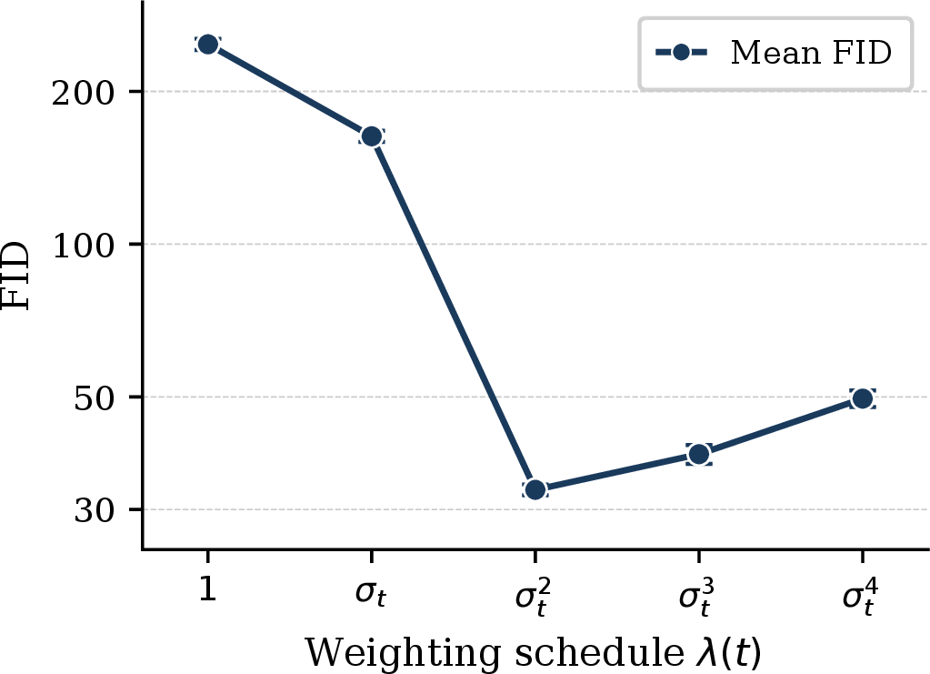
We examine the effect of the loss-weighting schedule \(\lambda(t)\) in the denoising score-matching objective by considering five choices: \(\lambda(t) \in \{1, \sigma_t, \sigma_t^2, \sigma_t^3, \sigma_t^4\}\) with uniform time sampling, i.e., \(q(t)=1\) for \(t \in [0,T]\). For each schedule, we train a separate model and evaluate generation quality using the Fréchet Inception Distance (FID) [45], keeping all other training and sampling settings fixed. This allows us to isolate the effect of the loss-weighting schedule on generation quality.

The results are reported in Figure 1. Since the optimization error contributes to the score-learning component of the generation error, the choice of \(\lambda(t)\) can influence the quality of the learned score function and, consequently, the quality of generated samples.

Consistently with the theoretical analysis, \(\lambda(t) = \sigma_t^2\) achieves the lowest FID among the schedules considered. This result can be interpreted as follows. For \(\lambda(t) = 1\) and \(\lambda(t) = \sigma_t\), the loss assigns insufficient weight to the small-noise regime, i.e., as \(t \to 0\), where the score is hardest to estimate and most critical for sample quality. This is consistent with our theoretical bound, which becomes large for small \(t\), and provides an additional explanation for the degraded performance and high FID observed under these schedules. Conversely, for \(\lambda(t) = \sigma_t^3\) and \(\lambda(t) = \sigma_t^4\), the weighting becomes excessively large in the high-noise regime, i.e., as \(t \to T\), concentrating the optimization effort on time steps where the signal-to-noise ratio is low and the score estimation is less informative for generation. As a result, the gradient signal at small \(t\) is relatively diminished, impairing fine-grained score estimation near the data distribution, leading to degraded sample quality compared to \(\sigma_t^2\).

The schedule \(\lambda(t) = \sigma_t^2\) provides a balanced trade-off between these two regimes: it avoids overweighting the high-noise regime, unlike \(\sigma_t^3\) and \(\sigma_t^4\), while assigning sufficient weight to the small noise regime to prevent gradient explosion and keep the optimization bound controlled. This is consistent with the signal-to-noise ratio weighting discussed in Section 4.2, where \(\lambda(t) = \sigma_t^2\) has been empirically shown to yield state-of-the-art generative performance. Overall, the empirical results are consistent with the theoretical analysis, which suggests that \(\lambda(t) = \sigma_t^2\) balances the optimization difficulty across noise levels. While this experiment is illustrative rather than exhaustive, it supports the view that this weighting is a natural choice from an optimization perspective.

6 Discussion↩︎

This paper provides score-approximation guarantees, and in particular optimization guarantees, for score-based generative models trained with SGD. For general score parameterizations, we show that SGD converges to an approximate stationary point of the weighted denoising score-matching objective, with explicit dependence on the schedule-dependent weighting factors. For overparameterized two-layer ReLU networks, our NTK analysis gives a direct bound on the score-approximation error along the SGD trajectory. This connects the optimization dynamics of denoising score matching to the score-learning term appearing in sampling guarantees, thereby clarifying how training error can affect the final sampling error. A main implication of our analysis is the role of the reweighting schedule. Our results provide theoretical guidance, from an optimization perspective, for weighting choices used in practice. One limitation is that our NTK analysis focuses on overparameterized two-layer ReLU networks. Although this setting helps us understand the optimization dynamics of diffusion models, extending the theory to deep U-Net architectures remains an important open question. A natural direction for future work is also to extend the present analysis to kinetic noising processes. In such models, the forward diffusion is augmented with a velocity variable, which may act as a powerful regularization mechanism. Empirically, kinetic SGMs often lead to improved generation error [7] but this improvement has not been proved by previous stability analyses [11], [14]. An interesting open problem is therefore to determine whether such a benefit can be captured within our framework through the score-learning term and the induced training dynamics.

7 Details and Proofs for the General SGD Analysis↩︎

7.1 Additional Details for SGD in Denoising Score Matching↩︎

In this section, we provide additional details on the stochastic gradient computation for denoising score matching. At each iteration \(k \in \mathbb{N}_*\), we independently sample \[X_0^{(k)} \sim \pi_{\rm data}, \qquad Z^{(k)} \sim \mathcal{N}(0,\mathbf{I}_d), \qquad t^{(k)} \sim q \,,\] and define \[\overrightarrow X_{t^{(k)}}^{(k)} = m_{t^{(k)}}X_0^{(k)}+\sigma_{t^{(k)}}Z^{(k)}, \qquad \overrightarrow\mathbf{U}^{(k)} := \bigl(\overrightarrow X_{t^{(k)}}^{(k)}, t^{(k)}\bigr)\in\mathbb{R}^d\times[0,T] \,.\] The stochastic gradient estimator at iteration \(k+1\) for a sample \(b\) is given by \[\begin{align} \label{eq:gradient95estimator95sample} g^{k+1}_{b} = \frac{c(t_b^{(k+1)})}{q(t_b^{(k+1)})} \Big(\nabla_{\theta}s_{\theta^{(k)}}(\overrightarrow\mathbf{U}^{(k+1)}_{b})\Big)^{\top} \Big(s_{\theta^{(k)}}(\overrightarrow\mathbf{U}^{(k+1)}_{b})+\frac{Z^{(k+1)}_{b}}{\sigma_{t^{(k+1)}_{b}}}\Big) \,. \end{align}\tag{18}\]

7.2 Proof of Theorem 1↩︎

8 Proof of the main NTK theorem↩︎

8.0.0.1 Probability space and conditioning.

The analysis involves three sources of randomness: the initialization \((A,\param^{(0)})\), the SGD sample iterations \[\mathbf{U}^{(k)}:=(X_0^{(k)},Z^{(k)},t^{(k)}), \qquad k\ge 0 \,,\] and independent fresh samples drawn from \(\overrightarrow\mathbf{U}:=(\overrightarrow X_{\tau}, \tau)\) used to evaluate the population quantities. Here, \(\overrightarrow\mathbf{U}\) has the same law as a training sample input, but is independent of both the initialization and the SGD sample stream. To avoid overloading notation, random variables sampled during SGD carry the iteration index in superscript, whereas fresh independent samples used only for evaluation are denoted with an arrow. We also introduce the corresponding filtrations, denoted by \[\mathcal{I} :=\sigma(A,\param^{(0)}) \,, \qquad \mathcal{F}_n :=\sigma(\mathbf{U}^{(0)},\dots,\mathbf{U}^{(n-1)}) \,, \qquad \mathcal{G}_n :=\sigma \left( \mathcal{I} \cup \mathcal{F}_n \right) \,.\] It follows that, for a fixed trained parameter \(\param^{(n)}\), the projected DSM loss is defined by \[\mathcal{L}_{\rm DSM}^{\Pi}(\param^{(n)}) := \frac{1}{2} \mathbb{E}\left[ c(\tau) \|\Delta_n^R( \overrightarrow\mathbf{U})\|^2 \,\middle| \mathcal{G}_n \right] \qquad \overrightarrow\mathbf{U}=(\overrightarrow X_\tau,\tau) \,.\] Throughout the rest of the proof, as in [38], we condition implicitly on \(\mathcal{I}\). When it is clear from the context, expectations are to be understood as with respect to the SGD sample stream only, or we specify \[\mathbb{E}_{\mathrm{sgd}} [ \cdot ] = \mathbb{E}[ \cdot | \mathcal{I} ] \,.\]

8.0.0.2 Localized DSM loss.

We first reduce the projected DSM loss to a localized \(L_2\) error plus a tail remainder. We introduce the truncated weighted measure \[\label{eq:def95mu95r} \mu_R(\mathrm{d}u) := c(t) q(t) p_t(x) \mathbf{1}_{\{\|x\|\le R\}} \mathrm{d}x \mathrm{d}t \,, \qquad u=(x,t) \in \mathbb{R}^{d} \times [0,T] \,.\tag{19}\] We define \[\begin{align} \label{eq:def95B95R} \mathcal{X}_R := \{(x,t)\in\mathbb{R}^d\times[0,T]:\|x\|\le R\}, \qquad B_R:=\sqrt{R^2+T^2} \,, \end{align}\tag{20}\] and we let \[\begin{align} \mu_R(\mathcal{X}_R) :=\int_0^T c(t) q(t) \mathbb{P}(\|\overrightarrow X_t\|\le R) \mathrm{d}t \,. \end{align}\]

8.0.0.3 Truncated SGD updates.

Fix an iteration horizon \(n\ge 1\) and a radius \(R>0\), and define \[\label{eq:good95event} \Omega_{n,R} := \bigcap_{k=0}^{n-1} \left\{ \|\overrightarrow X_{t^{(k)}}^{(k)}\| \le R \right\} \,.\tag{21}\] By the union bound, \[\mathbb{P} (\Omega_{n,R}^c) \le \sum_{k=0}^{n-1} \mathbb{P} \left(\|\overrightarrow X_{t^{(k)}}^{(k)}\|>R\right) = n \int_0^T q(t) \mathbb{P} (\|\overrightarrow X_t\|>R) \mathrm{d}t \,,\] which is controlled by Lemma 14. The NTK analysis is carried out on the good event \(\Omega_{n,R}\). We split \[\begin{align} \mathbb{E}_{\mathrm{sgd}}\!\left[\mathcal{L}_{\rm DSM}^{\Pi}(\param^{(n)})\right] &= \mathbb{E}_{\mathrm{sgd}}\!\left[\mathcal{L}_{\rm DSM}^{\Pi}(\param^{(n)}) \mathbf{1}_{\Omega_{n,R}}\right] + \mathbb{E}_{\mathrm{sgd}}\!\left[\mathcal{L}_{\rm DSM}^{\Pi}(\param^{(n)}) \mathbf{1}_{\Omega_{n,R}^c}\right] \,. \end{align}\] The first term is controlled by the localized error. Indeed, by ?? , \[\begin{align} \mathbb{E}_{\mathrm{sgd}} \left[ \mathcal{L}_{\rm DSM}^{\Pi}(\param^{(n)})\mathbf{1}_{\Omega_{n,R}} \right] & \le R\sqrt{\mu_R(\mathcal{X}_R)} \mathbb{E}_{\mathrm{sgd}}\!\left[ \|\Delta_n\|_{L_2(\mu_R)} \mathbf{1}_{\Omega_{n,R}} \right] \\ & \qquad + 2(1+C_0)R^2 \int_0^T c(t)q(t) \exp \left( -\frac{(R-\sigma_t\mu_Z)^2}{8\max(\sigma_t^2,m_t^2\nu_0^2)} \right)\mathrm{d}t \,. \end{align}\] To control the complement event, we use the trivial bound \[\|\Delta_n^R(u)\| \le \|\Pi_R(f^\star(u))\|+\|\Pi_R(f_\theta(u,\param[n]))\| \le 2R \,,\] which yields \[\begin{align} \mathbb{E}_{\mathrm{sgd}} \left[ \mathcal{L}_{\rm DSM}^{\Pi}(\param^{(n)})\mathbf{1}_{\Omega_{n,R}^c} \right] &\le 2R^2\left(\int_0^T c(t)q(t)\,\mathrm{d}t\right) \mathbb{P}(\Omega_{n,R}^c) \,. \end{align}\] Combining this with 21 and Lemma 14, \[\begin{align} \label{eq:bad95event95tail} \mathbb{P}(\Omega_{n,R}^c) &\le n(1+C_0) \int_0^T q(t) \exp\!\left( -\frac{(R-\sigma_t\mu_Z)^2}{8\max(\sigma_t^2,m_t^2\nu_0^2)} \right)\mathrm{d}t \,. \end{align}\tag{22}\] Therefore, \[\begin{gather} \mathbb{E}_{\mathrm{sgd}}\!\left[ \mathcal{L}_{\rm DSM}^{\Pi}(\param^{(n)})\mathbf{1}_{\Omega_{n,R}^c} \right] \\ \le 2(1+C_0)n R^2 \left(\int_0^T c(t)q(t)\,\mathrm{d}t\right) \left(\int_0^T q(t) \exp \left( -\frac{(R-\sigma_t\mu_Z)^2}{8\max(\sigma_t^2,m_t^2\nu_0^2)} \right)\mathrm{d}t\right) \,. \end{gather}\] In particular, with \(c_\infty :=\sup_{t\in[0,T]} c(t) < \infty\), we get \[\begin{align} \label{eq:equality95to95finsh95thm95295layers} \mathbb{E}_{\mathrm{sgd}} \left[ \mathcal{L}_{\rm DSM}^{\Pi}(\param^{(n)}) \right] & \le R\sqrt{\mu_R(\mathcal{X}_R)} \mathbb{E}_{\mathrm{sgd}} \left[ \|\Delta_n\|_{L_2(\mu_R)} \mathbf{1}_{\Omega_{n,R}} \right] \\ & \qquad + 2(1+C_0)c_\infty (n+1) R^2 \int_0^T q(t) \exp\!\left( -\frac{(R-\sigma_t\mu_Z)^2}{8\max(\sigma_t^2,m_t^2\nu_0^2)} \right) \mathrm{d}t \,. \end{align}\tag{23}\]

8.0.0.4 Localized error decomposition

We introduce the integral operators associated with the kernels \(K_k\) and \(K_\infty\), restricted to the localized region \(\mathcal{X}_R\). In particular, for every measurable function \(g:\mathbb{R}^{d} \times [0,T] \to\mathbb{R}^d\), \[\begin{align} (\mathsf K_k g)(u) & := \mathbb{E} \left[c(\tau)\,K_k(u,\overrightarrow\mathbf{U})\,g(\overrightarrow\mathbf{U}) \mathbf{1}_{\{\|\overrightarrow X_\tau\| \leq R\}} \right] \,, \qquad \overrightarrow\mathbf{U}=(\overrightarrow X_\tau,\tau) \,, \qquad \tau\sim q \,, \\ (\mathsf K_\infty g)(u) & := \mathbb{E}\left[c(\tau)\,K_\infty(u,\overrightarrow\mathbf{U}) g(\overrightarrow\mathbf{U}) \mathbf{1}_{\{\|\overrightarrow X_\tau\|\leq R\}} \right], \qquad \overrightarrow\mathbf{U}=(\overrightarrow X_\tau,\tau) \,, \qquad \tau\sim q \,. \end{align}\] We also introduce the following operators that will be useful throughout the proof: \[\begin{align} \label{eq:notation95kernel} \mathsf{P}_k := \mathsf{I}-\gamma_k \mathsf{K}_\infty \,,\qquad \mathsf{Q}_k := \mathsf{I} -\gamma_k \mathsf{K}_k \,, \qquad \mathsf{D}_k := \mathsf{Q}_k - \mathsf{P}_k \,, \end{align}\tag{24}\] where \(\mathsf{I}\) should be understood as the identity on \(L_2(\mu_R)\). In the following, all norms of vector-valued functions \(f: \mathbb{R}^{d} \times [0,T] \to \mathbb{R}^d\) are taken in \(L_2(\mu_R;\mathbb{R}^d)\), where \(\mu_R\) is defined in 19 : \[\|f\|^2_{L_2(\mu_R)} =\int \|f(u)\|^2 \mu_R(\mathrm{d}u) \,, \qquad u=(x,t)\in\mathbb{R}^{d} \times [0,T] \,.\] For a bounded linear operator \(\mathsf T\) on \(L_2(\mu_R;\mathbb{R}^d)\), we denote \[\|\mathsf T\|_{\rm op} =\sup_{\|f\|\le 1}\|\mathsf T f\|_{L_2(\mu_R)} \,.\]

8.1 Error decomposition↩︎

It now remains to bound each term in the above decomposition. For all \(n\ge 0\), define \[\begin{align} \mathcal{T}_{1,n} &:=\left\|\left(\prod_{k=0}^{n}\mathsf P_k\right)\Delta_0\right\|_{L_2(\mu_R)},\\ \mathcal{T}_{2,n} &:=\sum_{k=0}^{n}\|\mathsf D_k\|_{\rm op} \|\Delta_0\|_{L_2(\mu_R)},\\ \mathcal{T}_{3,n} &:=\left\| \sum_{k=0}^{n}\left(\prod_{r=k+1}^{n}\mathsf Q_r\right)v_k \right\|_{L_2(\mu_R)},\\ \mathcal{T}_{4,n} &:=\sum_{k=0}^{n}\|\varepsilon_k\|_{L_2(\mu_R)}. \end{align}\] Taking expectation with respect to the SGD sample stream, on the event \(\Omega_{n,R}\) conditionally on the initialization, yields \[\label{eq:expected95squared95error95decomp} \mathbb{E}_{\mathrm{sgd}} \left[\|\Delta_{n+1}\|_{L_2(\mu_R)} \mathbf{1}_{\Omega_{n+1,R}} \right] \le \sum_{\ell=1}^4 \mathbb{E}_{\mathrm{sgd}} \left[\mathcal{T}_{\ell,n} \mathbf{1}_{\Omega_{n+1,R}} \right] \,.\tag{25}\]

8.2 First term↩︎

For any function \(g \in L_2(\mu_R;\mathbb{R}^d)\), we denote by \(\mathcal{R}(g,r)\) the \(L_2(\mu_R;\mathbb{R}^d)\)-norm of the projection of \(g\) onto the subspace spanned by the eigenvectors \(\{e_i\}_{i=r+1}^\infty\), given by \[\begin{align} \label{eq:projection95K95infty} \mathcal{R}(g,r) := \left(\sum_{i=r+1}^{\infty} \langle g,e_i\rangle^2\right)^{1/2} \,. \end{align}\tag{26}\]

8.3 Second term↩︎

For a matrix-valued kernel \(G:\mathcal{X}_R\times\mathcal{X}_R\to\mathbb{R}^{d\times d}\), define \[\|G\|_{\infty,R} := \sup_{u,u'\in\mathcal{X}_R}\|G(u,u')\|\] and let \[\label{eq:def95loss95k} \mathbf{e}_k := f\left(\overrightarrow\mathbf{U}^{(k)};\param^{(k)}\right)-X_0^{(k)} = f\left(\overrightarrow\mathbf{U}^{(k)};\param^{(k)}\right) - \left(f^\star \left(\overrightarrow\mathbf{U}^{(k)}\right)+\xi_k\right) \,.\tag{27}\]

8.4 Third term↩︎

We let \[\sigma_k^2 := \mathbb{E}_{\mathrm{sgd}}\!\left[ \|\Delta_k\|_{L_2(\mu_R)}^2 \mathbf{1}_{\Omega_{k,R}} \right] +\tau_c^2 \,,\] where \(\tau_c^2 =\mathbb{E}\!\left[ c(\tau)\|\xi\|^2 \right]\) and \(\xi= X_0-f^\star(\overrightarrow X_\tau,\tau)\). For the \(k\)-th SGD sample, we write \[\xi_k := X_0^{(k)}-f^\star(\overrightarrow\mathbf{U}^{(k)}),\] so that \(\mathbb{E}[\xi_k\mid \overrightarrow\mathbf{U}^{(k)}]=0\) and therefore \[\label{eq:delta95sigma95relation} \mathbb{E}_{\mathrm{sgd}} \left[ c(t^{(k)}) \|\Delta_k(\overrightarrow\mathbf{U}^{(k)})+\xi_k\|^2 \mathbf{1}_{\Omega_{k+1,R}} \right] \le \mathbb{E}_{\mathrm{sgd}}\!\left[ \|\Delta_k\|_{L_2(\mu_R)}^2 \mathbf{1}_{\Omega_{k,R}} \right] + \mathbb{E}\left[c(\tau)\|\xi\|^2\right] = \sigma_k^2 \,.\tag{29}\]

8.5 Fourth term↩︎

8.6 Final bound↩︎

We prove by induction that for every \(0\le n\le N\), \[\label{eq:induction} \mathbb{E}_{\mathrm{sgd}}\!\left[ \|\Delta_n\|_{L_2(\mu_R)} \mathbf{1}_{\Omega_{n,R}} \right] \le S_N \,,\tag{37}\] with \[S_N := 2 \left( E_{1,N}+E_{2,N}+E_{3,N} \right) \,,\] where \[\begin{align} E_{1,N} & := \sup_{0\le j\le N} \inf_{r\in\mathbb{N}} \left\{ \left(\prod_{k=0}^{j-1}(1-\gamma_k\lambda_r)\right) \|\Delta_0\|_{L_2(\mu_R)} + \mathcal{R}(\Delta_0,r) \right\} \\ E_{2,N} & := C \mu_R(\mathcal{X}_R) B_R^2 d C_\gamma\log(N+1) \sqrt{\frac{d\log(m)+\log(1/\delta)}{m}} \sigma_0 \\ E_{3,N} & := C \left( 1+\sqrt{\frac{d}{m}} +\sqrt{\frac{\log(1/\delta)}{m}} \right)^2 \sqrt{c_\infty\mu_R} B_R^2 C_\gamma \mathrm{e}^{\Lambda_R C_\gamma} \left( 1+\frac{1}{1-2\Lambda_R C_\gamma} \right)^{1/2} \sigma_0 \,. \end{align}\] Once this is proven, Theorem 2 follows from 23 .

The base case \(n=0\) is immediate. Now suppose that 37 holds for all \(0\le k\le n\). We prove that it also holds for \(n+1\). By 25 , we obtain \[\begin{align} \mathbb{E}_{\mathrm{sgd}} \left[\|\Delta_{n+1}\|_{L_2(\mu_R)} \mathbf{1}_{\Omega_{n+1,R}} \right] \le \mathbb{E}_{\mathrm{sgd}} [ \left(\mathcal{T}_{1,n}+\mathcal{T}_{2,n}+\mathcal{T}_{3,n}+\mathcal{T}_{4,n}\right)\mathbf{1}_{\Omega_{n+1,R}}] \,. \end{align}\] For the first term, Lemma 5 gives \[\begin{align} \mathbb{E}_{\mathrm{sgd}} \left[ \mathcal{T}_{1,n}\mathbf{1}_{\Omega_{n+1,R}} \right] &\le \inf_{r\in\mathbb{N}}\left\{ \left(\prod_{k=0}^{n}(1-\gamma_k\lambda_r)\right) \|\Delta_0\|_{L_2(\mu_R)} + \mathcal{R}(\Delta_0,r) \right\} \,. \end{align}\] For the second term, using Lemma 6, together with the Cauchy–Schwarz inequality and the fact that \(\gamma_k = C_\gamma/(k+1)\), we obtain \[\begin{align} & \mathbb{E}_{\mathrm{sgd}} \left[ \mathcal{T}_{2,n} \mathbf{1}_{\Omega_{n+1,R}} \right] \\ &\le C \mu_R(\mathcal{X}_R) B_R^2 \|\Delta_0\|_{L_2(\mu_R)} \Bigg[ \frac{d^{3/2} B_R}{\sqrt{m}} \mathbb{E}_{\mathrm{sgd}} \left[ \left(\sum_{k=0}^{n} \gamma_k \eta_k \right) \mathbf{1}_{\Omega_{n+1,R}} \right] \\ &\qquad\qquad + d \sqrt{\frac{d\log(m)+\log(1/\delta)}{m}} \sum_{k=0}^{n}\gamma_k \Bigg] \\ &\le C \mu_R(\mathcal{X}_R) B_R^2 \|\Delta_0\|_{L_2(\mu_R)} \Bigg[ \frac{d^{3/2} B_R}{\sqrt{m}} C_\gamma \log (\mathrm{e}(N+1)) \sum_{k=0}^{n} \gamma_k \mathbb{E}_{\mathrm{sgd}} \left[\|\Delta_k\|_{L_2(\mu_R)}+\tau_c\right] \\ &\qquad\qquad + d \sqrt{\frac{d\log(m)+\log(1/\delta)}{m}} C_\gamma \log (N+1) \Bigg] \,. \end{align}\] Indeed, by the definition of \(\eta_k\) and using the fact that, for all \(r\le k-1\le n\), one has \(\Omega_{n+1,R}\subset \Omega_{r+1,R}\subset \Omega_{r,R}\), we have \[\begin{align} \mathbb{E}_{\mathrm{sgd}}\left[ \left(\sum_{k=0}^{n}\gamma_k\eta_k\right) \mathbf{1}_{\Omega_{n+1,R}} \right] &\le \sum_{k=0}^{n}\gamma_k \sum_{r=0}^{k-1}\gamma_r \mathbb{E}_{\mathrm{sgd}}\left[ c(t^{(r)})\|\mathbf{e}_r\| \mathbf{1}_{\Omega_{n+1,R}} \right] \\ &\le \sum_{k=0}^{n}\gamma_k \sum_{r=0}^{k-1}\gamma_r \mathbb{E}_{\mathrm{sgd}}\left[ c(t^{(r)})\|\mathbf{e}_r\| \mathbf{1}_{\Omega_{r+1,R}} \right] \\ &\le \sqrt{\mu_R(\mathcal{X}_R)} \sum_{k=0}^{n}\gamma_k \sum_{r=0}^{k-1}\gamma_r ( \mathbb{E}_{\mathrm{sgd}} \left[\|\Delta_{r}\|_{L_2(\mu_R)} \mathbf{1}_{\Omega_{r,R}} \right] +\tau_c) \,. \end{align}\] Under the induction hypothesis \(\mathbb{E}_{\mathrm{sgd}}\!\left[ \|\Delta_r\|_{L_2(\mu_R)}\mathbf{1}_{\Omega_{r,R}} \right] \le S_N\), therefore \[\begin{align} \mathbb{E}_{\mathrm{sgd}}\!\left[ \left(\sum_{k=0}^{n}\gamma_k\eta_k\right) \mathbf{1}_{\Omega_{n+1,R}} \right] &\le \sqrt{\mu_R(\mathcal{X}_R)} (S_N+\tau_c) \left(\sum_{k=0}^{n}\gamma_k\right)^2 \\ &\le \sqrt{\mu_R(\mathcal{X}_R)} C_\gamma^2 \log^2(\mathrm{e}(N+1)) (S_N+\tau_c) \,. \end{align}\] By the width condition \(m \ge c \mu_R^3(\mathcal{X}_R) B_R^6 d^3 C_\gamma^4 \log^4 (N+1)\) for a sufficiently large constant \(c>0\), the first contribution can be absorbed into the induction bound. Therefore, \[\begin{align} \mathbb{E}_{\mathrm{sgd}} \left[ \mathcal{T}_{2,n} \mathbf{1}_{\Omega_{n+1,R}} \right] \le C \mu_R(\mathcal{X}_R) B_R^2 d C_\gamma \log (N+1) \sqrt{\frac{d\log(m)+\log(1/\delta)}{m}} \left(\|\Delta_0\|_{L_2(\mu_R)}+\tau_c\right) \,. \end{align}\] For the third term, Lemma 11 gives \[\begin{align} & \mathbb{E}_{\mathrm{sgd}} \left[ \mathcal{T}_{3,n} \mathbf{1}_{\Omega_{n+1,R}} \right] \\ &\le C\left( 1+\sqrt{\frac{d}{m}} +\sqrt{\frac{\log(1/\delta)}{m}} \right)^2 \sqrt{c_\infty \mu_R(\mathcal{X}_R)} B_R^2 C_{\gamma} e^{\Lambda_R C_{\gamma}} \left(1+\frac{1}{1-2\Lambda_R C_\gamma}\right)^{1/2} \sigma_0 \,. \end{align}\] For the fourth term, using the induction bound, for all \(0\le k\le n\), we have \[\begin{align} \mathbb{E}_{\mathrm{sgd}} [\eta_{k+1} \mathbf{1}_{\Omega_{n+1,R}}] &\leq \sqrt{\mu_R(\mathcal{X}_R)} C_\gamma \log(\mathrm{e}(N+1)) (S_N+\tau_c) \,. \end{align}\] Using Lemma 12, we obtain \[\begin{align} &\mathbb{E}_{\mathrm{sgd}}\left[\mathcal{T}_{4,n}\mathbf{1}_{\Omega_{n+1,R}}\right] \\ &\quad \le C dB_R^2\sqrt{c_\infty\mu_R(\mathcal{X}_R)} \left( \frac{B_R\sqrt{d\mu_R(\mathcal{X}_R)}}{\sqrt m} C_\gamma \log(\mathrm{e}(N+1))S_N + \sqrt{\frac{d+\log(1/\delta)}{m}} \right)^{1/2} \sum_{k=0}^{n}\gamma_k\sigma_k \,. \end{align}\] Moreover, \[\sum_{k=0}^{n}\gamma_k\sigma_k \le C_\gamma e^{\Lambda_R C_\gamma}\sigma_0 \frac{(N+1)^{\Lambda_R C_\gamma}}{\Lambda_R C_\gamma} = \frac{e^{\Lambda_R C_\gamma}}{\Lambda_R} \sigma_0 (N+1)^{\Lambda_R C_\gamma} \,.\] Using the definition of \(\Lambda_R\), we have \[\frac{dB_R^2\sqrt{c_\infty\mu_R(\mathcal{X}_R)}}{\Lambda_R} = \frac{d}{d+\|A\|^2/m} \le 1 \,.\] Therefore, \[\begin{align} &\mathbb{E}_{\mathrm{sgd}}\left[\mathcal{T}_{4,n}\mathbf{1}_{\Omega_{n+1,R}}\right] \\ &\quad \le C e^{\Lambda_R C_\gamma} \sigma_0 (N+1)^{\Lambda_R C_\gamma} \left( \frac{B_R\sqrt{d\mu_R(\mathcal{X}_R)}}{\sqrt m} C_\gamma \log(\mathrm{e}(N+1)) (S_N+\tau_c) + \sqrt{\frac{d+\log(1/\delta)}{m}} \right)^{1/2} \,. \end{align}\] Using \(\sqrt{x+y}\le \sqrt{x}+\sqrt{y}\), we get \[\mathbb{E}_{\mathrm{sgd}}\left[\mathcal{T}_{4,n}\mathbf{1}_{\Omega_{n+1,R}}\right] \le I_1+I_2 \,,\] where \[\begin{align} I_1 &= C e^{\Lambda_R C_\gamma} \sigma_0 (N+1)^{\Lambda_R C_\gamma} \left( \frac{B_R\sqrt{d\mu_R(\mathcal{X}_R)}}{\sqrt m} C_\gamma \log(\mathrm{e}(N+1)) (S_N+\tau_c) \right)^{1/2} \,, \\ I_2 &= C e^{\Lambda_R C_\gamma} \sigma_0 (N+1)^{\Lambda_R C_\gamma} \left(\frac{d+\log(1/\delta)}{m}\right)^{1/4} \,. \end{align}\] By definition of \(S_N\), and by increasing the universal constant if necessary, \[S_N \ge c \sqrt{c_\infty\mu_R(\mathcal{X}_R)} B_R^2 C_\gamma e^{\Lambda_R C_\gamma} \sigma_0 \,,\] for some universal constant \(c>0\). Moreover, the imposed width condition \[m \ge c \frac{ e^{2\Lambda_R C_\gamma} \sigma_0^2 (N+1)^{4\Lambda_R C_\gamma} d\log^2(\mathrm{e}(N+1)) }{ c_\infty B_R^2 }\] implies that \[C e^{2\Lambda_R C_\gamma} (N+1)^{2\Lambda_R C_\gamma} \frac{B_R\sqrt{d\mu_R(\mathcal{X}_R)}}{\sqrt m} C_\gamma \log(\mathrm{e}(N+1)) \le c \sqrt{c_\infty\mu_R(\mathcal{X}_R)} B_R^2 C_\gamma e^{\Lambda_R C_\gamma} \sigma_0 \le S_N \,.\] Therefore, \[\begin{align} I_1^2 &= C e^{2\Lambda_R C_\gamma} (N+1)^{2\Lambda_R C_\gamma} \frac{B_R\sqrt{d\mu_R(\mathcal{X}_R)}}{\sqrt m} C_\gamma \log(\mathrm{e}(N+1)) S_N \le S_N^2/4 \,. \end{align}\] Consequently, \[I_1\le S_N/2 \,.\] Similarly, other width condition gives \[m \ge c \frac{ (N+1)^{4\Lambda_R C_\gamma} (d+\log(1/\delta)) }{ c_\infty^2\mu_R(\mathcal{X}_R)^2B_R^8C_\gamma^4 } \,.\] Equivalently, \[I_2 = C e^{\Lambda_R C_\gamma} \sigma_0 (N+1)^{\Lambda_R C_\gamma} \left(\frac{d+\log(1/\delta)}{m}\right)^{1/4} \le c \sqrt{c_\infty\mu_R(\mathcal{X}_R)} B_R^2 C_\gamma e^{\Lambda_R C_\gamma} \sigma_0 \le S_N/2 \,.\] Combining the bounds on \(I_1\) and \(I_2\), we obtain \[\mathbb{E}_{\mathrm{sgd}}\left[\mathcal{T}_{4,n}\mathbf{1}_{\Omega_{n+1,R}}\right] \le S_N \,,\] This completes the fourth term. Thus, under the width condition \[\begin{gather} \label{eq:condition95width} m \ge c \max\Bigg\{ \mu_R^2(\mathcal{X}_R) B_R^6 d^3 C_\gamma^4 \log^4 (N+1),\; \frac{(N+1)^{4\Lambda_R C_\gamma}(d+\log(1/\delta))}{c_\infty^2\mu_R(\mathcal{X}_R)^2B_R^8C_\gamma^4} , \\ \frac{e^{2\Lambda_R C_\gamma} (N+1)^{4\Lambda_R C_\gamma} d\log^2(\mathrm{e}(N+1))}{c_\infty B_R^2} \Bigg\} \,, \end{gather}\tag{38}\] the induction bound holds at iteration \(n+1\). For readability, this condition can be summarized by introducing \[\begin{align} \label{eq:def95C95R} \mathcal{C}_R :=\max\left\{ \mu_R^3(\mathcal{X}_R)B_R^6C_\gamma^4, \frac{1}{c_\infty^2\mu_R^2(\mathcal{X}_R)B_R^8C_\gamma^4}, \frac{1}{c_\infty\mu_R(\mathcal{X}_R)B_R^2} \right\} \,. \end{align}\tag{39}\] Indeed, a sufficient condition for 38 is \[m \gtrsim \mathcal{C}_R e^{2\Lambda_R C_\gamma} (N+1)^{4\Lambda_R C_\gamma} d^3 \bigl(d+\log(1/\delta)\bigr) \log^4(\mathrm{e}(N+1)) \,.\] This concludes the proof of Theorem 2.

9 Additional Derivations for the NTK Analysis↩︎

Recall that, \[\mathbf{e}_k := f\left(\overrightarrow\mathbf{U}^{(k)};\param^{(k)}\right)-X_0^{(k)} = f\left(\overrightarrow\mathbf{U}^{(k)};\param^{(k)}\right) - \left(f^\star \left(\overrightarrow\mathbf{U}^{(k)}\right)+\xi_k\right) \,.\]

9.1 Details on the Neural Tangent Kernel↩︎

For every \(u\in\mathbb{R}^{d+1}\), we define the empirical matrix-valued NTK, \(K_k:\mathbb{R}^{d+1}\times\mathbb{R}^{d+1}\to\mathbb{R}^{d\times d}\) by \[\begin{align} K_k(u,u') &:= \sum_{i=1}^m \nabla_{\param_i}f(u;\param[k])\, \nabla_{\param_i}f(u';\param[k])^\top \notag\\ &= \frac{u^\top u'}{m} \sum_{i=1}^m \mathbf{1}_{\{(\param[k]_i)^\top u\ge 0\}} \mathbf{1}_{\{(\param[k]_i)^\top u' \ge 0\}} \,A_{\cdot i}A_{\cdot i}^\top \notag\\ &= \frac{u^\top u'}{m}\, A\,D_{u,\param[k]}D_{u',\param[k]}A^\top . \label{eq:empirical95matrix95ntk} \end{align}\tag{40}\]

It follows that, \[f(u;\param[k+1]) = f(u;\param[k]) - \gamma_k c(t^{(k)}) K_k(u,\overrightarrow\mathbf{U}^{(k)}) \mathbf{e}_k - \varepsilon_k(u, \overrightarrow\mathbf{U}^{(k)}) \,, \label{eq:one95step95linearization}\tag{41}\] where \[\varepsilon_k(u, \overrightarrow\mathbf{U}^{(k)}) :=f(u;\param[k]) -f(u;\param[k+1]) - \gamma_k c(t^{(k)}) K_k(u,\overrightarrow\mathbf{U}^{(k)}) \mathbf{e}_k \label{eq:def95linearization95error}\tag{42}\] is a nonlinear remainder. It measures the error made when replacing the exact one-step update of the network output by its first-order NTK approximation.

At initialization, the empirical matrix-valued NTK admits a deterministic infinite-width limit. More precisely, assume that \[\{\param_i^{(0)}\}_{i=1}^m \overset{\mathrm{i.i.d.}}{\sim} \mathcal{N}(0,\mathbf{I}_{d+1}),\] independently of the output matrix \(A\), whose entries are i.i.d. Rademacher. Then, for every fixed \(u,u'\in\mathbb{R}^{d+1}\), \[K_0(u,u') = \frac{u^\top u'}{m} \sum_{i=1}^m \mathbf{1}_{\{(\param_i^{(0)})^\top u\ge 0\}} \mathbf{1}_{\{(\param_i^{(0)})^\top u' \ge 0\}} \,A_{\cdot i}A_{\cdot i}^\top \xrightarrow[m\to\infty]{a.s.} K_\infty(u,u') \,.\] with \[K_\infty(u,u') = (u^\top u')\, \mathbb{E}_{w \sim \mathcal{N}(0,\mathbf{I}_{d+1})} \Big[ \mathbf{1}\{w^\top u\ge 0\}\, \mathbf{1}\{w^\top u' \ge 0\} \Big]\, \mathbf{I}_d\] since \(\mathbb{E}[A_{\cdot i}A_{\cdot i}^\top]=\mathbf{I}_d\).

9.2 SGD Update Derivation↩︎

For simplicity, we introduce \(\mathbf{e}_k \in \mathbb{R}^d\) defined by \[\begin{align} \mathbf{e}_k :=f\left(\overrightarrow\mathbf{U}^{(k)};\param^{(k)}\right)-X_0^{(k)} = f\left(\overrightarrow\mathbf{U}^{(k)};\param^{(k)}\right) - \left(f^\star \left(\overrightarrow\mathbf{U}^{(k)}\right)+\xi_k\right) \,. \end{align}\] where \[\begin{align} \overrightarrow\mathbf{U}^{(k)} :=\bigl(\overrightarrow X_{t^{(k)}}^{(k)},t^{(k)}\bigr), \qquad \xi_k :=X_0^{(k)}-f^\star\!\bigl(\overrightarrow\mathbf{U}^{(k)}\bigr) \,. \end{align}\]

9.3 Technical Lemmas↩︎

Let \[\begin{align} I_i^0(u)=\mathbf{1}\{\param_i^{(0)\top}u\ge0\}, \qquad p(u,u')= \mathbb{E}_{\param\sim\mathcal{N}(0,\mathbf{I}_{d+1})} \left[ \mathbf{1}\{\param^\top u\ge0\} \mathbf{1}\{\param^\top u'\ge0\} \right] \,. \end{align}\]

References↩︎