A Large-Scale Sparse Multiobjective Optimization Algorithm Based on Optimal Performance Scores
July 06, 2026
Abstract
Large-scale sparse multiobjective optimization problems (LSSMOPs) involve a large number of decision variables and Pareto optimal solutions with only a few nonzero variables. However, as the number of decision variables grows, it becomes increasingly challenging to accurately identify the nonzero variables, and optimization performance is adversely affected. To address these issues, this paper proposes an evolutionary algorithm for LSSMOPs. Specifically, we propose a new initialization method capable of generating scores that accurately reflect the importance of variables, and an initial mask vector template that can locate nonzero variables. This leads to the generation of a high-quality initial population. Additionally, this paper introduces a new strategy to calculate the mutation probability for each variable and a novel optimization for real variables based on the Pareto-guided normal distribution, enabling the population to avoid being trapped in local optima and quickly converge to the global optimum. Experimental results from eight benchmark problems and three real-world applications demonstrate that the proposed algorithm achieves superior performance compared with state-of-the-art algorithms.
,Multiobjective optimization ,Sparse optimization ,Evolutionary algorithm ,Optimal performance scores
1 Introduction↩︎
Multiobjective optimization plays a central role in many fields [1], such as machine learning [2], [3], data mining [4], and financial decision making [5], aiming to
optimize multiple (often conflicting) performance criteria simultaneously and to obtain the Pareto front (PF). Pareto optimal solutions of sparse multiobjective optimization problems (SMOPs) contain only a few nonzero variables. SMOPs have direct
engineering relevance in a variety of applications [6], including feature selection [7], where one seeks a compact subset of informative features to improve model interpretability and predictive performance; sparse signal reconstruction [8], which aims to recover an accurate signal from limited or noisy measurements by exploiting its inherent sparsity; and sparse neural network training [9], which enforces weight sparsity so that most network parameters become zero and the resulting model is smaller to store. In SMOPs, we
seek solutions that are both close to the PF and as sparse as possible, to satisfy practical constraints like interpretability, storage, and computational cost.
With the rapid growth of data scale and system complexity, large-scale sparse multiobjective optimization algorithms (LSSMOOAs) have become increasingly common: decision-variable dimensionality can be extremely high, but in many practical problems, only a
small subset of variables dominantly affects objectives (i.e., solutions are sparse). This sparsity is both a challenge and an opportunity – exploiting sparse structure can dramatically reduce the search space and evaluation cost, while ignoring it often
leads conventional algorithms to suffer from the curse of dimensionality or poor efficiency [10].
Conventional multiobjective evolutionary algorithms (MOEAs) perform well on small-scale benchmark problems but encounter three major bottlenecks on large-scale SMOPs [11]–[13]. First, random variation and standard crossover make
it difficult to find key variable combinations in high-dimensional spaces, leading to low search efficiency [14], [15]. Second, function evaluations are often expensive, and thus repeated evaluations of high-dimensional solutions become prohibitive [16]. Third, maintaining both convergence and diversity becomes harder under sparsity constraints [17], [18]: algorithms may converge to dense or local optimal solutions [19]. Recent advances – such as sparsity-aware operators [20], variable selection heuristics [21], neural network model based dimensionality reduction method [22], [23], and multi-stage knowledge guidance [24] – have partially
addressed these problems, but important limitations remain: many methods rely on static or heuristic variable selection rules that fail to track changes in variable importance during the searc [25], [26]; others lack effective coordination between neural network models and
population structure, which limits scalability and robustness in real large-scale tasks. [27]–[29]
To address these challenges, this paper proposes an algorithm that can efficiently optimize binary vectors and real vectors. Specifically, the main contributions are as follows:
In this paper, we propose a new initialization framework that can be easily embedded into other algorithms. The scores of the variables are calculated based on their performance in all intervals of the decision space, which can more accurately reflect the importance of the variables. Based on these scores, an initial mask vector template can be generated, which guides the initial population to locate the nonzero variables. The values of the real variables are sampled in the appropriate intervals according to their performance in different intervals. Therefore, the initialization method can generate a high-quality initial population that accurately identifies the nonzero variables.
We propose an adaptive mutation probability for each real variable and a Pareto-guided resampling strategy based on the normal distribution. The mutation scheme sets the mutation probability for each real variable based on its behavior across all intervals, assigning higher probabilities to variables that are more prone to becoming trapped in local optima. The Pareto-guided resampling strategy facilitates the generation of real vectors of Pareto optimal solutions.
The proposed large-scale sparse multiobjective optimization algorithm based on optimal performance scores, abbreviated as SMOEA-OPS, is used to compare with the state-of-the-art on eight benchmark problems and three real-world problems. The experiments demonstrate that SMOEA-OPS achieves significantly better performance than competing algorithms.
The rest of this paper is organized as follows. In Section II, some basic concepts of sparse multiobjective optimization problems, existing LSSMOOAs, and the motivation of this work are given. In Section III, the proposed algorithm is described in detail. In Section IV, the experimental results on benchmark and real-world SMOPs are presented and analyzed. Finally, the conclusions are described in Section V.
2 Related work↩︎
2.1 Sparse multiobjective optimization↩︎
The unconstrained multiobjective optimization problem can be defined mathematically as follows: \[\min_{\mathbf{x} \in\mathbb{R}^D} \quad \mathbf{F}(\mathbf{x}) = \left( f_1(\mathbf{x}),\, f_2(\mathbf{x}),\, \dots,\, f_m(\mathbf{x}) \right)\] where \(\mathbf{x} = (x_1, x_2, \dots, x_D)^\mathrm{T}\) denotes the decision vector in a \(D\)-dimensional search space, and \(\mathbf{F}(\mathbf{x})\) represents the objective vector consisting of \(m\) conflicting objective functions \(f_i(\mathbf{x})\), \(i = 1, \dots, m\). The goal of multiobjective optimization problems is to find a set of Pareto optimal solutions, for which no objective can be improved without degrading at least one other objective [30]. The concept of Pareto dominance is used to compare solutions. Given two decision vectors \(\mathbf{x}^a\) and \(\mathbf{x}^b\), we say that \(\mathbf{x}^a\) dominates \(\mathbf{x}^b\), denoted by \(\mathbf{x}^a \prec \mathbf{x}^b\), if and only if the following two conditions hold:
\(f_i(\mathbf{x}^a) \lef_i(\mathbf{x}^b)\) for all \(i \in\{1, \dots, m\}\),
\(f_j(\mathbf{x}^a) < f_j(\mathbf{x}^b)\) for at least one index \(j \in\{1, \dots, m\}\).
a solution is called Pareto optimal if it is not dominated by any other solution in the search space. The set of all Pareto optimal solutions is known as the Pareto set (PS).
Sparse multiobjective optimization, on the other hand, means that only a few decision variables in the decision vectors of the Pareto optimal solutions are nonzero, i.e., the number of meaningful variables is much smaller than the total number of decision
variables \(D\). When dealing with LSSMOPs (\(D\) \(\ge\)100), conventional MOEAs often suffer from prohibitive computational costs due to the curse of
dimensionality and the difficulty of effectively identifying the influential variables [31]. To address these challenges, a variety
of sparse multiobjective optimization algorithms have been developed.
2.2 Initialization for solving LSSMOPs↩︎
Existing algorithms for tackling sparse problems typically use one of three initialization strategies [32]: random sampling, Latin hypercube
sampling [33], or the sparse population approach. For example, S-ECSO [34] and PM-MOEA [35] use random initialization, i.e., the initial \(N\) individuals are generated at random positions in the decision space. There are also a few algorithms initialized by the Latin hypercube sampling method, such as MOEA/PSL [22].
However, the majority of LSSMOOAs employ the sparse population approach, which was originally proposed by the first sparse MOEA – SparseEA [36]. SparseEA first introduced representing an individual \(\mathbf{x}\) using a real vector \(dec\) and a binary vector \(mask\), i.e., a two-layer encoding scheme, as given by the following formula: \[\mathbf{x} = \big( dec_1\timesmask_1,\; \dots,\; dec_D\timesmask_D \big)\] where \(D\) denotes the dimension of the solutions. In SparseEA, the initialization begins by constructing \(D\) sparse solutions through the two-layer encoding strategy. In each of these solutions,
only one decision variable is set to a nonzero value, while all others are fixed at zero. These \(D\) solutions are evaluated and ranked according to Pareto dominance, and a score is assigned to each decision variable based
on the non-dominated front number of its associated single-variable solution. From these scores, we can generate a binary mask matrix that determines the active variables in each individual. This binary mask matrix is then combined element-wise with a
randomly generated real-valued matrix to form the initial population.
However, the scores produced by SparseEA can be unreliable. Recent methods such as MGCEA [37] and KLEA [38] address this by splitting each domain of decision variables into multiple equal subintervals and sampling within each interval. For each variable, MGCEA computes the score by aggregating
its non-dominated front number across all sampled intervals. By evaluating a variable’s performance throughout its range rather than at random ranges, this multi-interval sampling yields more robust and accurate scores for constructing a sparse initial
population.
2.3 Real vectors optimization for LSSMOPs↩︎
Most LSSMOPs now adopt a two-layer encoding that represents a solution with a hybrid of a real vector and a binary vector. While most LSSMOOAs focus on handling sparsity via mask encodings without directly optimizing the real variables, a few algorithms specifically address convergence on the real vector component. For example, SparseEA2 [39] enhances the mask–real interplay via variable grouping to ensure nonzero variables are more thoroughly optimized. MOEA/PSL achieves dimensionality reduction through autoencoder-based subspaces, where real vectors are optimized in a learned low-dimensional domain. MSKEA [24], S-ECSO, and PM-MOEA incorporate dynamic sparse knowledge or convex operators to guide the real vector toward Pareto optimal. Furthermore, rank-1 approximation-based EAs [40] decompose the real vector into subspaces via tensor decomposition and optimize them alternately, enabling more efficient convergence.
2.4 Motivation of this work↩︎
The scoring mechanism used by SparseEA fails to provide a reliable measure of variable importance, since it does not consider the full distribution of each variable’s values within the decision space. MGCEA computes each variable’s score by summing its non-dominated front numbers across all intervals. However, this score calculation method also tends to ignore some variables that have potential. As shown in Fig. 1, the non-dominated front number of the first variable in the third interval is very small, i.e., this variable is very promising. But the sum of the non-dominated front numbers in all intervals makes the score of this variable very large, which can easily result in overlooking this variable, especially in some complex landscapes.
To enable subsequent individuals to evolve based on more accurate scores, this paper considers a new method for computing scores. In this paper, each variable’s score is determined by the lowest non-dominated front number it attains over the decision
space. The non-dominated front numbers of each variable across all intervals are recorded in the matrix \(IntervalFronts\). This matrix can also guide which interval each real variable should be sampled from, thereby
producing high-quality initial solutions.
Since only a very small number of LSSMOOAs consider the optimization of real vectors, this paper proposes a Pareto-guided resampling method based on the normal distribution for optimizing real vectors. We divide the evolution into two stages according to
the number of decision variables. In stage one, we preserve the diversity of the real vectors; in stage two, we intensify resampling to steer solutions toward the Pareto set.

3 The proposed SMOEA-OPS↩︎
3.1 The framework of SMOEA-OPS↩︎

The SMOEA-OPS framework is shown in Algorithm 1. First, we initialize to obtain the population \(P\), the vector \(Score\), and a boolean flag indicating whether the \(initMask\) is informative. In the main loop, \(2N\) parents are selected in \(P\) using the strategy of SPEA2 [41] to generate offspring. The vector \(Score\) is used to measure the importance of each decision variable across the solution set; smaller values indicate higher importance. To avoid premature convergence to local optima caused by always using high-quality solutions from the current population to guide offspring, we use the ratio of consumed evaluations as the probability to update \(Score\). Before updating \(Score\), update the vector \(Sparsity\) as follows: \[Sparsity_i = \frac{1}{|PS|}\sum_{p\inPS} pb_i \label{eq:sparsity}\tag{1}\] where \(Sparsity_i\) is the sparsity of the \(i\)-th variable, \(pb_i\) is the \(i\)-th variable of the binary vector of solution \(p\) in Pareto optimal solutions. Then the score of the \(i\)-th variable of the current generation is updated:
\[\small Score_i = Score_i' + \lambda(Sparsity_{max}-Sparsity_i) \label{eq:score}\tag{2}\] where \(Score_i'\) refers to the score of
\(i\)-th variable before it is updated, \(Sparsity_{max}\) denotes the maximum sparsity among all variables in binary vectors, and \(\lambda\) denotes the
ratio of consumed evaluations, i.e., \(FE/FE_{max}\). \(FE\) and \(FE_{max}\) represent the current and the maximum number of evaluations, respectively. As
the number of function evaluations increases, the scores of zero variables increase much faster than those of nonzero variables, causing the nonzero variables to become increasingly distinguishable. The probability of updating the \(Score\) vector becomes larger as it gets further into the evolutionary process. This enables learning towards high-quality Pareto optimal solutions and achieves the effect of exploration in the early stage and exploitation in
the later stage.
Then we compute \(\mu\) and \(\sigma\) (the mean and standard deviation of each real variable across the current Pareto set) and use them to make offspring learn from the Pareto set. The
\(i\)-th entry of \(\mu\) is calculated as: \[\mu_i = \frac{1}{|PS|} \sum_{p \inPS} pr_i\] where \(pr_i\) denotes the \(i\)-th real variable of solution \(p\) in the Pareto set. The \(i\)-th element of \(\sigma\) is computed as:
\[\sigma_i = \sqrt{\frac{1}{|PS|}\sum_{p\inPS}\big(pr_i - \mu_i\big)^2} \label{eq:sigma}\tag{3}\] Then, a population \(Q\) is generated through
variation and resampling. Afterward, population \(Q\) is combined with \(P\). \(N\) solutions are selected from the combined population to survive to the
next generation through the environmental selection strategy of SPEA2.
3.2 The proposed initialization approach↩︎

The initialization framework is shown in Algorithm 2. The vector \(Score\) and the matrix \(IntervalFronts\) are first calculated using Algorithm 3. The \(flag\) indicates whether \(initMask\) is informative. The mask template \(initMask\) is used to guide the generation of the binary vectors of the initial
population. If all elements of \(initMask\) are zero, it provides little guidance, and \(flag\) is set to 1. The generation of population T, from which \(initMask\) is derived, is described in Lines 5–13 of Algorithm 2 (see Fig. 2 for an example).
First, \((ln D)-1\) iterations are carried out, where \(D\) denotes the number of decision variables, and the loop index \(i\) starts at \(2\). In each iteration, \(K\)-means is first applied to partition all variables into \(i\) groups based on their scores. Variables in the group with the smallest
mean score are set to \(1\), while variables in the remaining groups are set to \(0\). From each iteration, \(N / ((lnD)-1)\) identical mask vectors are
produced, so that after all iterations a total of \(N\) mask vectors are obtained. Meanwhile, \(N\) real vectors are generated based on \(IntervalFronts\).
The calculation of \(IntervalFronts\) and the generation of solutions will be described in Algorithm 3 and Algorithm 4, respectively. Subsequently, the \(N\) mask vectors and the \(N\) real vectors are combined to form a population \(T\) of size \(N\), which is then utilized to generate an \(initMask\) for
the initialization of the population’s binary vectors. The population \(T\) not only maintains sparsity but also activates the most promising variables.

![Figure 5: Illustrative example of generating a population T. Assume real variables range over [0,2], lnD=3, and NVal=4. In the binary vectors, darker shading indicates higher variable scores within a group. In each column of the IntervalFronts matrix, lighter shading corresponds to a smaller non-dominated front number for the associated variable in that interval — in other words, lighter entries make the variable more likely to take a value from that interval.](/article/2607.04765/figs/popT.png "fig:")

To obtain mask vectors that more accurately identify nonzero variables, an initial mask template \(initMask\) is computed from the population \(T\) and the variable-score vector \(Score\); this template is used to guide the generation of initial mask vectors. If all elements of the computed \(initMask\) are zero, \(T\) is used directly as
the initial population; otherwise, \(initMask\) and \(IntervalFronts\) are used separately to generate \(N\) mask vectors and \(N\) real vectors for the initial solutions.
The maximum number of groups is set to \(ln D\) because it adapts to \(D\): as the number of decision variables \(D\) increases, partitioning becomes finer.
Moreover, \(ln D\) grows much more slowly than \(D\), keeping \(ln D\) within a reasonable range as \(D\) varies and thereby
reducing computational cost.
Algorithm 3 details the method for calculating \(Score\) during the initialization phase. The \(Front\) calculation is similar to the multi-interval sampling [37] proposed by MGCEA, which allows the total non-dominated front numbers of each variable across the entire interval to be taken into account when calculating \(Score\). The range of the real value of the \(c\)-th variable in the \(m\)-th iteration is as follows: \[\begin{align} Dec_{\cdot c} \in& \left[ lower_c + \frac{(upper_c - lower_c)\times(m-1)}{NVal}, \right. \\ & \left. lower_c + \frac{(upper_c - lower_c)\timesm}{NVal} \right] \end{align} \label{zonhgtsj}\tag{4}\]
where \(lower_c\) and \(upper_c\) are the lower and upper bounds of the \(c\)-th real variable, respectively.
However, if we simply add up the non-dominated front numbers of all intervals to calculate the scores may overlook potential variables. When certain variables perform exceptionally well in one interval but poorly in others, the score obtained by adding up
the non-dominated front numbers of all intervals may be high, resulting in the variable being eliminated. To solve this problem, the non-dominated front numbers of each variable in the \(NVal\) intervals should be retained
as \(IntervalFronts\). For example, \(IntervalFronts_{i,j}\) denotes the sum, over \(SVal\) runs of non-dominated sorting, of the non-dominated front numbers
of solutions in interval \(i\) drawn from the solution sets where only variable \(j\) is nonzero. To explain more clearly, Fig. 3 shows an example of the initialization of \(Score\). First, the matrix \(IntervalFronts'\) is obtained by dividing each element of the \(IntervalFronts\) matrix by the maximum element value in its
corresponding row. Then, the minimum value in each column of \(IntervalFronts'\), corresponding to that variable’s score at its optimal performance, is used to form the vector \(Score\).
The lower a variable’s score, the more important that variable tends to be.
The population generated during initialization is shown in Algorithm 4. Higher-quality solutions can be generated in the initialization by using \(IntervalFronts\) to guide the generation of real vectors, and \(initMask\) to guide the generation of binary vectors. When generating real vectors, each variable should be sampled with high probability in the interval with a low non-dominated front number. So the probability that the \(j\)-th variable is sampled from the \(intv\)-th interval is given as follows: \[\large intvProb_{j,intv} =
\frac{\frac{1}{IntervalFronts_{intv,j}}}{\sum_{i=1}^{NVal}\frac{1}{IntervalFronts_{i,j}}}\] where \(NVal\) is the number of intervals. Taking \(IntervalFronts\) of Fig. 3 as an
example, the probability that the 2-th real variable is sampled in the 3-th interval is \(\frac{1}{18}/(\frac{1}{8}+\frac{1}{18}+\frac{1}{56}+\frac{1}{145})\). In this case, each real variable has a greater chance of
generating real values in the range where it performs well, thereby obtaining good real vectors. For binary vectors, the value of each variable in the mask template represents the probability that the corresponding variable should be set to 1 when
generating binary vectors.

To find promising variables, this paper proposes a function shown in Algorithm 5. As shown in Fig. 4, to avoid losing promising variables, the Pareto optimal solutions are selected from population \(T\) to compute \(initMask\). For each selected solution, we iteratively generate new solutions by setting the highest-scoring nonzero element in the mask vector to zero at each step. If the new solution dominates the original solutions, it
indicates that the variables previously set to 0 are less important, and the operation is repeated. If an original solution dominates the new solution, it indicates that the variable set to 0 is important, and the loop operation is terminated. After
repeating the above procedure for all Pareto optimal solutions in population \(T\), a set of non-dominated solutions is obtained. Then sum their binary vectors element-wise and divide by the total number of non-dominated
solutions to obtain \(initMask\). Each element of \(initMask\) represents the probability that the corresponding position element of the initial binary vector is 1.


3.3 Genetic operators of SMOEA-OPS↩︎

As shown in Algorithm 6, the genetic operators of SMOEA-OPS have a similar framework to SparseEA. First, randomly select two parents p and q from \(P\) to generate offspring o each time, and set the binary vector of o to be the same as that of p. Then, one of the following two crossover operations is chosen with equal probability: select a nonzero element from \(\boldsymbol{p}.mask\cap\boldsymbol{q}.\overline{mask}\), where the selection probability of each element is computed by Eq.(9). Then, set the corresponding element in \(\boldsymbol{o}.mask\) to \(0\); or select a nonzero element from \(\boldsymbol{p}.\overline{mask}\cap\boldsymbol{q}.mask\), where the selection probability of each element is computed by Eq.(10). Then, set the corresponding element in \(\boldsymbol{o}.mask\) to \(1\). Specifically, during the crossover operation, the probability that the \(j\)-th element of offspring o is selected and assigned 0 can be calculated as follows:
\[P_{j,0}^{C} = \frac{Score_j}{\sum_{idx\inC_1} Score_{idx}} \label{eq:pc0}\tag{5}\] where \(C_1\) denotes the intersection of the nonzero
elements between p.\(mask\) and q.\(\overline{mask}\). Meanwhile, the probability that the \(j\)-th element of offspring o is selected and assigned 1 can be calculated as follows: \[P_{j,1}^{C} = \frac{\frac{1}{Score_j}}{\sum_{idx\inC_0}
\frac{1}{Score_{idx}}} \label{yimwecuv}\tag{6}\] where \(C_0\) denotes the intersection of the nonzero elements between p.\(\overline{mask}\) and q.\(mask\).
Since the mask vectors obtained after population initialization can accurately activate most of the important variables, the mutation probability of mask vectors can be gradually reduced as evolution progresses, which also helps optimize the real variables
and reduces computational cost. Specifically, the mutation probability of mask vectors is set to dynamically change as \(1 - \lambda\), where \(\lambda\) is the ratio of consumed
evaluations, i.e., \(FE/FE_{max}\). When o.mask mutates, one of the following two operations is performed with the same probability: select an element from the nonzero entries of o.\(mask\) with probabilities given by Eq.(11), and set it to 0; or select an element from the nonzero entries of \(\mathrm{\boldsymbol{o}}.\overline{mask}\) with probabilities given by Eq.(12), and set it to 1. Specifically, during the mutation operation, the probability that the \(j\)-th element of
offspring o is selected and assigned 0 can be calculated as follows: \[P_{j,0}^{M} = \frac{Score_j}{\sum_{idx\inM_1} Score_{idx}} \label{ibqxkjfc}\tag{7}\] where
\(M_1\) denotes the set of nonzero elements from o.\(mask\). Meanwhile, the probability that the \(j\)-th element is selected and assigned 1
can be calculated as follows: \[P_{j,1}^{M} = \frac{\frac{1}{Score_j}}{\sum_{idx\inM_0} \frac{1}{Score_{idx}}} \label{ymanufwg}\tag{8}\] where \(M_0\) denotes the set of zero elements from o.\(mask\).
The real vector o\(.dec\) of solution o is generated by simulated binary crossover [42] and polynomial mutation [43], similar to most MOEA. In this paper, the mutation probability of each real
variable is proportional to the standard deviation of values in the corresponding column of \(IntervalFronts\). The calculation of \(IntervalFronts\) is described in Lines 2–16 of Algorithm
3. The formula for calculating the standard deviation of the elements in the \(j\)-th column of \(IntervalFronts\) is as follows: \[std_j = \sqrt{\frac{1}{NVal-1}\sum_{i=1}^{NVal}{(IntervalFronts_{i,j} - \overline{IntervalFronts_{:,j}})^2}} \label{eq:std}\tag{9}\]
where \(\overline{IntervalFronts_{:,j}}\) represents the average value of all the elements in the \(j\)-th column of the matrix \(IntervalFronts\).
Therefore, the formula for calculating the mutation probability of the \(j\)-th real variable in the solution r can be written as follows:
\[mutProb_{\boldsymbol{r},j} = \begin{cases} \frac{std_j}{\sum_{k\innz\_idx}std_k}, & \boldsymbol{r}.mask_{j} \neq0,\\[6pt] 0 & \boldsymbol{r}.mask_{j} = 0 \end{cases}
\label{eq:mut}\tag{10}\] where \(nz\_idx\) denotes the set of indices of nonzero elements from r\(.mask\). As the population evolves, the number of nonzero
elements gradually decreases. The term \(\sum_{k\innz\_idx} std_k\), which excludes the standard deviations of the zero elements in the current solution, increases the mutation probability of all nonzero variables in
solution r. If the \(j\)-th element of the mask vector of r is \(0\), the corresponding real variable does not need to mutate, and its mutation probability
is therefore set to \(0\).
This probability scheme also prevents real variables from being sampled only within the intervals with the smallest non-dominated front numbers, thereby improving diversity and reducing the risk of getting trapped in local optima.
3.4 The proposed Pareto-guided resampling strategy for optimizing real vectors↩︎
Many LSSMOOAs focus only on the optimization of binary vectors and ignore the optimization of real vectors, resulting in poor performance. Therefore, this paper proposes a Pareto-guided resampling method based on the normal distribution for optimizing real vectors, as shown in Algorithm 7. When dealing with LSMOPs, their complex search landscapes typically require strong early-stage exploration to maintain diversity. Therefore, the evolutionary process is divided into two stages according to the number of decision variables. In the first stage, the population’s exploration ability is maintained, whereas in the second stage, its convergence toward the Pareto set is further strengthened.
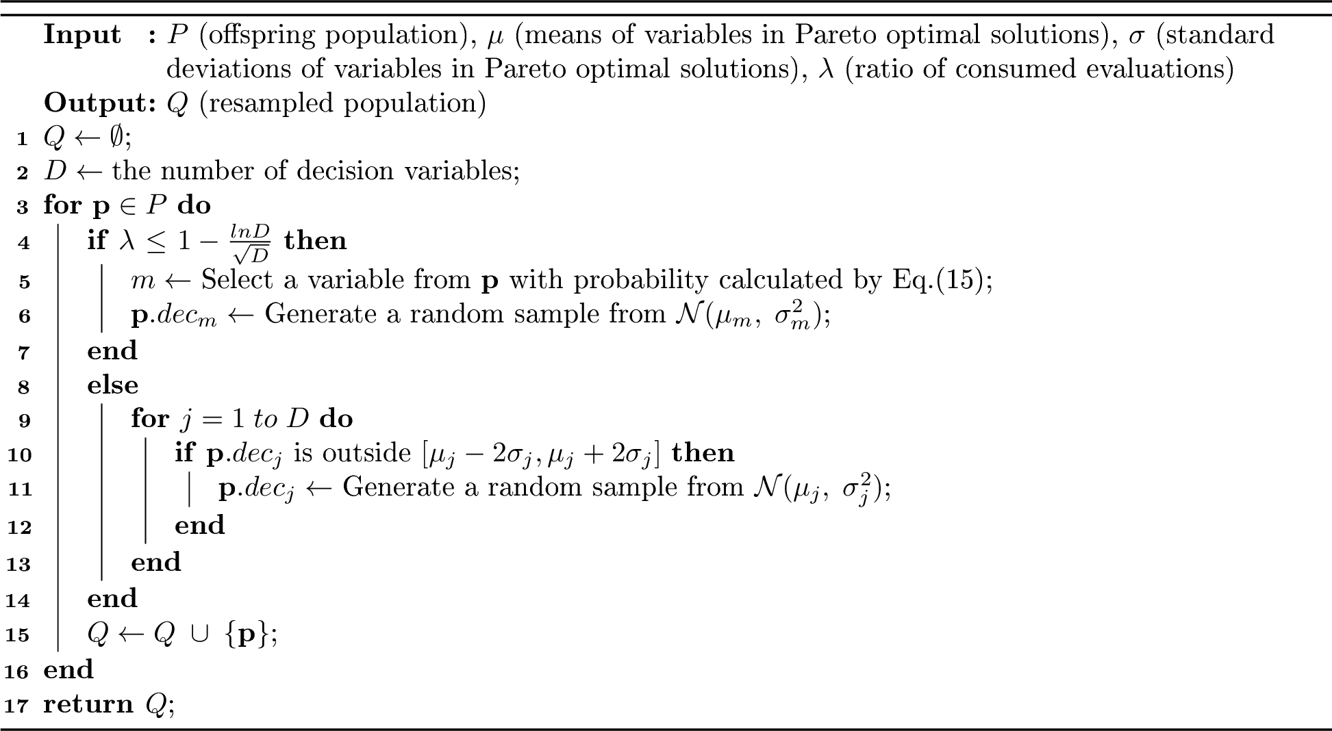
In the early stage, for each solution, a variable is selected with the probability proportional to its standard deviation in the current population. The probability of the \(i\)-th variable being selected is calculated
as follows: \[resampleProb_i = \frac{\sigma_i}{\sum_{j=1}^{D}\sigma_j} \label{zjmhevan}\tag{11}\] where \(\sigma_i\) and \(D\) represent the standard deviation of the \(i\)-th variables in Pareto optimal solutions and the number of decision variables, respectively. In the first stage, if the \(i\)-th variable is selected in a solution, draw a sample from the normal distribution \(\mathcal{N}(\mu_i,\sigma_i^2)\) and assign it to the \(i\)-th variable.
Therefore, in the first stage, by resampling only those offspring’s real variables that deviate excessively from the Pareto set, the population’s diversity is preserved. In the second stage, all real variables of the population learn from the current
Pareto set (Algorithm 7, lines 8–10): all real variables that deviate from the Pareto set are resampled to strengthen offspring convergence toward the Pareto set. Specifically, for each solution, if there exists \(j\in\{1,\dots,D\}\) such that the \(j\)-th variable lies outside the interval \([\mu_j-2\sigma_j,\;\mu_j+2\sigma_j]\), then resample the \(j\)-th variable from \(\mathcal{N}(\mu_j,\sigma_j^2)\).
As the number of decision variables grows, locating Pareto-optimal solutions becomes more difficult. To increase the chance of escaping local optima, we therefore extend the exploration phase for higher-dimensional problems. Concretely, we split the
evolutionary process so that the initial \((1 - \frac{lnD}{\sqrt{D}})\%\) of the run focuses on the exploration, while the final \(\frac{lnD}{\sqrt{D}}\%\) of the run concentrates on the
exploitation. We reserve the final \(\frac{lnD}{\sqrt{D}}\%\) of the evolutionary process for exploitation because this ratio can adaptively change as the dimension changes: \(lnD\) grows
slowly, while \(\sqrt{D}\) grows faster than \(lnD\) but not as fast as \(D\), causing the overall ratio to shrink with \(D\) without collapsing too abruptly. Thus, in higher-dimensional problems, the exploration stage can be extended to improve the chances of finding high-quality solutions. Moreover, as \(D\)
varies across problems, \(\frac{lnD}{\sqrt{D}}\) remains within a reasonable range.
4 Experimental results↩︎
To evaluate the performance of SMOEA-OPS, eight benchmark problems, namely SMOP1-SMOP8 [36], and three real-world SMOPs are used
to verify the obtained solutions. Real-world SMOPs introduce problems with real-valued decision spaces and binary decision spaces, namely, sparse signal reconstruction (SR) [8], community detection (CD) [22], and the knapsack problem (KP) [44]. Moreover, SparseEA2 [39],
S-NSGA-II [45], MSKEA [24],
TELSO [46], MGCEA [37] are selected as baseline
algorithms. All experiments were conducted on PlatEMO [47].
4.1 Settings of algorithms↩︎
The parameters of the compared MOEAs are set to the values recommended in their original papers. For SparseEA2, the number of groups is set to 4. For MGCEA and the proposed SMOEA-OPS, the number of intervals \(NV al\) is
set to 5, and the number of samplings per interval \(SV al\) is set to 2.
Simulated binary crossover [42] and polynomial mutation [43] are used to generate the real variables of offspring solutions for SparseEA2, MSKEA, MGCEA, and the proposed SMOEA-OPS. For algorithms other than SMOEA-OPS, the crossover and mutation probabilities are set to \(\,1\,\) and \(\,1/D\,\), respectively. The distribution indices for crossover and mutation are both set to 20. S-NSGA-II and TELSO use their own genetic operators to generate real variables for
offspring solutions. In particular, S-NSGA-II generates real variables within [0, 1] and rounds them to obtain binary variables [37].
The population size is set to 100 in both the benchmark SMOPs and the real-world SMOPs. The maximum number of function evaluations is set to \(100 \timesD\) on benchmark problems. For real-world SMOPs, the maximum number of
function evaluations is set to \(20\timesD\) for SR1-SR4, 20000 for CD1-CD4, and \(100\timesD\) for KP1-KP4.
4.2 Settings of problems↩︎
| problem | ||||||
| variables | ||||||
| variables | ||||||
| objectives | ||||||
| Pareto optimal solutions | sec: | sec: | ||||
| SMOP1–SMOP8 | Real | 100 | 2 | 0.1 | ||
| 500 | ||||||
| 1000 | ||||||
| 5000 | ||||||
| reconstruction problem | ||||||
| variables | ||||||
| variables | Dataset | |||||
| signal | ||||||
| signal | ||||||
| signal | ||||||
| SR1 | Real | 1024 | Synthetic [8] | 1024 | 512 | 256 |
| SR2 | 2048 | Synthetic [8] | 2048 | 1024 | 512 | |
| SR3 | 3072 | Synthetic [8] | 3072 | 1536 | 768 | |
| SR4 | 4096 | Synthetic [8] | 4096 | 2048 | 1024 | |
| problem | ||||||
| variables | ||||||
| variables | Dataset | |||||
| CD1 | Binary | 34 | Karate1 | 34 | 78 | |
| CD2 | 62 | Dolphin1 | 62 | 159 | ||
| CD3 | 105 | Polbook1 | 105 | 441 | ||
| CD4 | 115 | Football1 | 115 | 613 | ||
| variables | ||||||
| variables | Dataset | sec: | sec: | |||
| KP1 | Binary | 100 | Synthetic [44] | 100 | ||
| KP2 | 500 | Synthetic [44] | 500 | |||
| KP3 | 1000 | Synthetic [44] | 1000 | |||
| KP4 | 5000 | Synthetic [44] | 5000 |


For the eight benchmark problems SMOP1–SMOP8, the number of objectives is set to 2, the number of decision variables \(D\) is set to 100, 500, 1000, and 5000, and the sparsity of Pareto optimal solutions is set to 0.1.
The three real-world SMOPs are included in PlatEMO 4.8. Details can be found in Table 1.
To evaluate the performance of the algorithms, inverted generational distance (IGD) [48] and hypervolume (HV) [49] are used to assess the performance of each algorithm in 30 independent runs on benchmark problems and practical problems, respectively. As
shown in Table 2, “\(+\)” indicates that an algorithm performs better than the proposed SMOEA-OPS, “\(-\)” indicates that an algorithm performs worse than the proposed SMOEA-OPS, and “\(\approx\)” indicates that an algorithm performs similarly to the proposed SMOEA-OPS.

4.3 Comparative experiments↩︎


Figure 14: Objectives values of the population with average IGD among 30 runs obtained by SparseEA2, MSKEA, S-NSGA-II, TELSO, MGCEA and the proposed SMOEA-OPS on SMOP2, SMOP5 and SMOP7 with 1000 variables..


Figure 15: Parallel coordinates of the decision variables obtained by the proposed SMOEA-OPS on SMOP1, SMOP2, SMOP3, and SMOP7 at the 11-th generations. All the variables outside the pink region should be set to zero in the Pareto optimal solutions..
The optimization results for SMOEA-OPS and the five comparison algorithms are given in Table 2. It is clear that SMOEA-OPS attains the best performance on SMOP1, SMOP2, SMOP3, SMOP5, SMOP6 and SMOP7. Among the 32 test instances, SMOEA-OPS achieves the
best results in 22 cases. Specifically, SMOEA-OPS outperforms SparseEA2, MSKEA, S-NAGA-II, TELSO, and MGCEA on 31, 26, 31, 28, and 19 test instances, respectively.
Fig. 5 shows the parallel coordinate plots [50] of the final decision variables produced by the proposed SMOEA-OPS and the comparison algorithms on
SMOP1, SMOP2, and SMOP7. For these problems, Pareto optimal solutions require the first 11 decision variables to be nonzero [36].
It is clear that only SMOEA-OPS and MGCEA accurately identify the nonzero decision variables. SparseEA2 returns solutions that are not sparse enough, while MSKEA, S-NSGA-II, and TELSO produce incomplete solutions – for example, the final population of
S-NSGA-II for SMOP1 includes solutions with the 9-th variable equal to zero. Compared to MGCEA, the final population produced by SMOEA-OPS more accurately approximates the true Pareto front of the SMOPs: nonzero decision variables concentrate tightly
around the expected values. For example, on SMOP1, the second through 11-th decision variables in the final solutions of SMOEA-OPS cluster precisely near \(\pi/3\) [36], while the corresponding variables in the solutions of MGCEA do not converge to this target. This superior performance is mainly attributed to the Pareto-guided resampling method based
on the normal distribution proposed in this paper. These results indicate that SMOEA-OPS can obtain high-quality solutions.
To provide a visual confirmation of SMOEA-OPS’s superiority, Fig. 6 shows the IGD convergence curves of SMOEA-OPS and the compared algorithms on SMOP1, SMOP2, and SMOP7 with 100 decision variables. In all three cases, SMOEA-OPS converges much earlier,
attaining the IGD values that other algorithms only reach at later stages, and achieves the lowest IGD at the end of the run. Fig. 7 presents the objective values of the population obtained by the six algorithms on SMOP2, SMOP5, and SMOP7 with 1000
decision variables. Across these problems, SMOEA-OPS outperforms the competing algorithms, achieving superior convergence toward the PF while also maintaining greater diversity. Fig. 8 presents the populations obtained at the 5700-th generation, i.e.,
after 11% of the evaluation budget (5,700 out of 50,000), from a single run of SMOEA-OPS on SMOP1, SMOP2, SMOP3, and SMOP7 with 500 decision variables. These results show that, even right after initialization, SMOEA-OPS’s population accurately and
comprehensively identifies the nonzero decision variables while maintaining the desired sparsity.
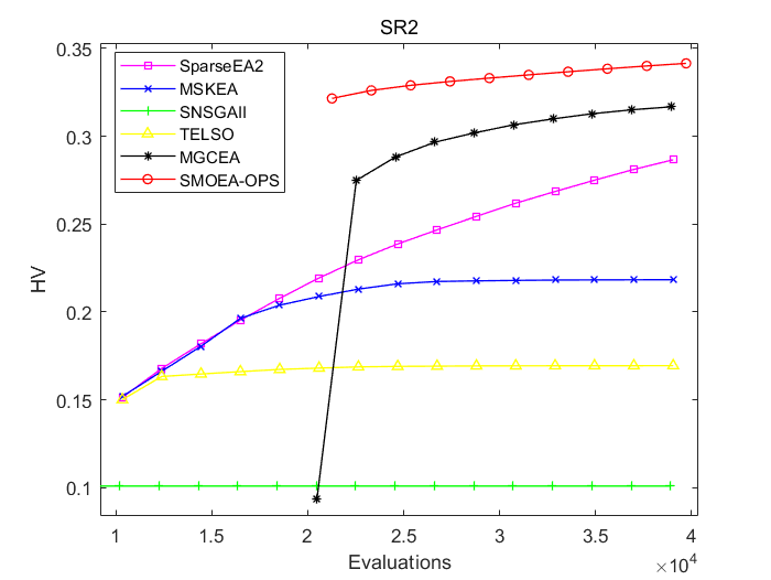
Table 3 reports the mean and standard deviation of HV computed from 30 independent runs for each of the six MOEAs on the practical problems SR1–SR4, KP1–KP4, and CD1–CD4. SMOEA-OPS outperforms all other algorithms on every test instance except CD4,
where it performs similarly to MSKEA. In addition, Fig. 9 presents the HV curves on SR2, which show that the population produced by SMOEA-OPS at initialization achieves a higher HV than the final populations of the five competing algorithms. This
demonstrates the superiority of the initialization method used in SMOEA-OPS.
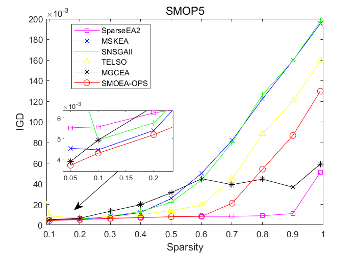
Fig. 10 plots the average IGD curves of six algorithms among 30 runs on SMOP5 with 100 decision variables as the sparsity parameter varies from 0.05 to 1. The results show that when the sparsity is below \(\,0.7\,\), SMOEA-OPS achieves lower IGD than the other five algorithms. Overall, the results indicate that SMOEA-OPS performs better on sparser problems and remains reasonably robust across different sparsity levels.
4.4 Ablation studies↩︎
5pt
mean of IGD values among 30 runs obtained by SMOEA-OPS, SMOEA-OPS’, SMOEA-OPS”, and SMOEA-OPS”’ on SMOP1–SMOP8 with 100 decision variables.
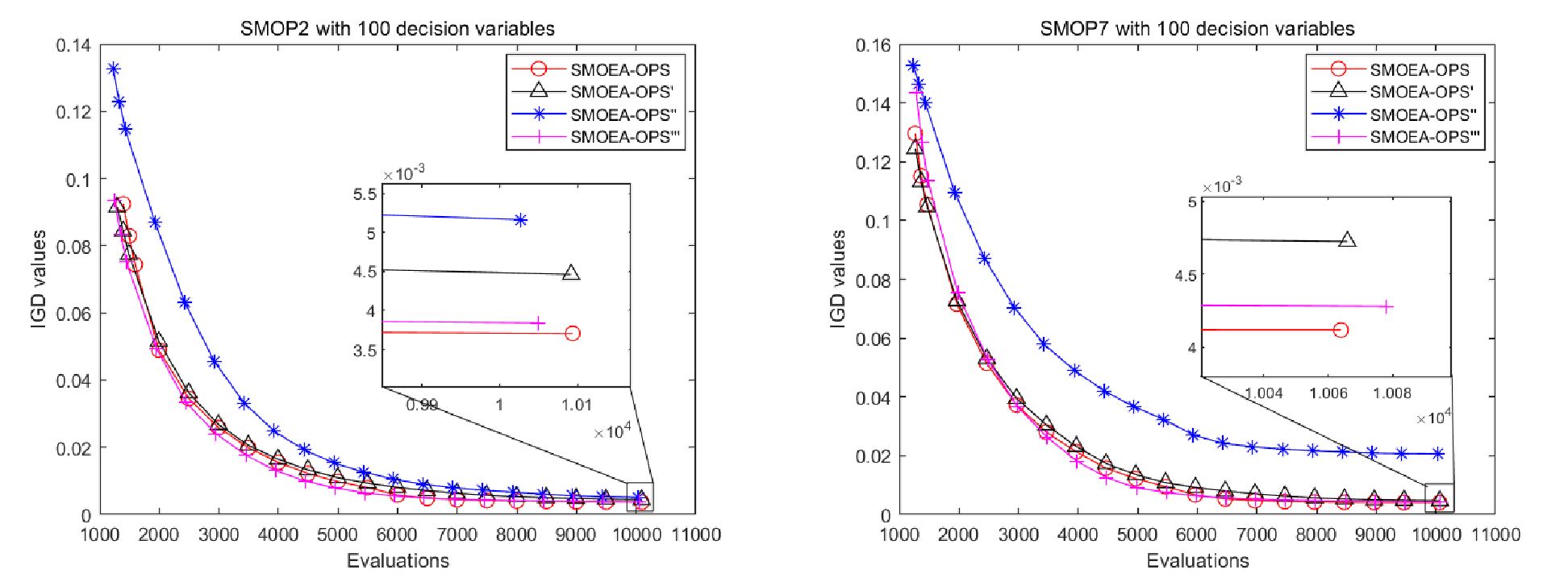
SMOEA-OPS’s superior performance is mainly attributed to three components: the Pareto-guided resampling method based on the normal distribution for optimizing real vectors, the new score of variable computation, and the dynamic mutation probabilities
assigned to each real variable for different solutions. To demonstrate the contribution of these three components to the optimization results, three variants of SMOEA-OPS are proposed for ablation experiments, namely SMOEA-OPS\('\), SMOEA-OPS\(''\), and SMOEA-OPS\('''\). SMOEA-OPS\('\) is obtained by removing the Pareto-guided
resampling in SMOEA-OPS. SMOEA-OPS\(''\) is obtained by replacing the \(Score\) with the sum of the non-dominated front numbers of the \(NVal\)
intervals in SMOEA-OPS, which is the score calculated by the MGCEA method. SMOEA-OPS\('''\) is obtained by replacing \(mutProb\) with \(1/D\) as
the variance probability of real variables.
Table 4 shows the mean and standard deviation of the IGD obtained by SMOEA-OPS and variants of SMOEA-OPS on the SMOP benchmark problem with 100 decision variables. The deterioration of the optimization results can be observed through the three variants of
SMOEA-OPS due to the absence of these three components.
Fig. 11 visually illustrates the convergence profiles in terms of IGD values for SMOEA-OPS and its three variants. SMOEA-OPS achieves a faster decrease in IGD than SMOEA-OPS\('\) and SMOEA-OPS\(''\). SMOEA-OPS\('''\) achieves a faster decrease in IGD than SMOEA-OPS, but its final solutions are inferior. This is because SMOEA-OPS’s \(mutProb\) encourages stronger exploration in the early stages, enabling the algorithm to escape local optima and obtain better final solutions. Overall, SMOEA-OPS\('\) performs worst, which
shows the importance of the proposed Pareto-guided resampling strategy. On SMOP7, SMOEA-OPS\(''\) records a much higher IGD than the others, indicating that the proposed calculation of score is effective on
high-difficulty problems with both epistasis and multimodal landscapes [38].
4.5 Sensitivity analysis↩︎
The vector \(Score\) is calculated based on \(SVal\) and \(NVal\) like MGCEA. Fig. 12 shows a heatmap of the total IGD across SMOP1–SMOP8 for varying NVal
and SVal, with 100 decision variables and 2 objectives. Note that to avoid the IGD of SMOP8 dominating the results, divide the SMOP8 value by 10 in advance. We can conclude from Fig. 12 that when \(NVal\) and \(SVal\) take 5 and 2, respectively, the sum of IGD across SMOP1-SMOP8 is the lowest, that is, the algorithm performs the best. If \(SVal\) and \(NVal\) are
further increased, it will result in more evaluations being consumed. Therefore, \(NVal\) and \(SVal\) are set to 5 and 2, respectively.

2pt
Means of runtime (in second) among 30 runs obtained by SparseEA2, MSKEA, S-NSGA-II, TELSO, MGCEA, and the proposed SMOEA-OPS on SMOP1–SMOP8.
4.6 Computational efficiency↩︎
Table 5 shows a comparison of the runtimes of the proposed SMOEA-OPS and the other five algorithms. The results show that the proposed SMOEA-OPS is competitive with MGCEA and SparseEA2. For the higher-dimensional KP4 problem, whose solutions are represented as binary vectors, SMOEA-OPS has a runtime that is outperformed only by SparseEA2 and MSKEA due to its use of relatively simple genetic operators. In summary, S-NSGA-II has the shortest runtime on most problems, followed by TELSO. The runtimes of the other four algorithms are comparable. However, S-NSGA-II and TELSO yield the worst optimization results, whereas SMOEA-OPS obtains the best results within a reasonable running time.
5 Conclusions↩︎
LSSMOPs are still very challenging, mainly because most LSSMOOAs do not obtain populations that can accurately cover nonzero variables after initialization. Consequently, the population typically requires extended evolution or a large number of
expensive function evaluations to discover the relevant variables. This paper proposes A large-scale sparse multiobjective optimization algorithm based on optimal performance scores. Specifically, this paper proposes three key techniques: a new
initialization strategy, a dynamic mutation-probability calculation based on the performance of real variables across intervals, and a Pareto-guided resampling method based on the normal distribution for optimizing real vectors. The proposed initialization
method produces initial populations that accurately cover the nonzero variables. The proposed mutation probability and Pareto-guided resampling improve real vector optimization and enable the algorithm to escape local optima. These three components can be
easily embedded into other algorithms. Finally, we validate SMOEA-OPS on a suite of eight benchmark SMOPs and three real-world SMOPs; the results show that SMOEA-OPS is consistently effective and achieves superior performance.
In future work, we aim to further reduce the function evaluation cost incurred during initialization, thereby preserving a larger share of the evaluation budget for subsequent evolutionary search. We will replace the manual parameters \(NVal\) and \(SVal\) with an adaptive, problem-driven computation. Moreover, we will explore more efficient methods for optimizing real variables in LSSMOPs to mitigate the computational overhead
introduced by resampling.
CRediT authorship contribution statement↩︎
Jia-Lin Mai: Writing - review & editing, Writing - original draft, Software, Conceptualization, Formal analysis. Min-Rong Chen: Methodology, Writing - original draft, Writing - review & editing, Funding acquisition. Guo-Qiang Zeng: Supervision, Funding acquisition. Xiang Liu: Supervision, Writing - review & editing, Funding acquisition. Jian Weng: Project administration, Funding acquisition.
Declaration of competing interest↩︎
The authors declare that they have no known competing financial interests or personal relationships that could have appeared to influence the work reported in this paper.
Acknowledgement↩︎
This work was supported in part by the National Natural Science Foundation of China (Grant Nos. 62573201, U23A20303, 62573326, 62533016, 61825203, 62332007, and U22B2028), in part by the Zhejiang Provincial Natural Science Foundation of China (Grant No. LZ25F030007), in part by the Outstanding Youth Project of Guangdong Basic and Applied Basic Research Foundation (Grant No. 2023B1515020064), and in part by the Guangdong Basic and Applied Basic Research Foundation (Grant No:2024A1515140109).