1 Motivation↩︎

Sparsity, i.e., the prevalence of a large number of zeros or near-zero values in data, is common in certain parallel workloads, including high performance computing [1]–[4], but even more so in distributed deep learning [5]–[8]. Exploiting sparsity in data (both application input data and large matrices in memory) for improving the performance of computation and communication is common [9]–[11]. Communication optimizations center on sending only important information (e.g. nonzero values), often in collective operations such as all-gather, reduce-scatter, and all-reduce. As communication overheads in parallel applications can represent a significant fraction of execution time, particularly as applications scale to more GPUs and nodes, such optimizations can be particularly helpful for large messages and at high GPU counts.

Historically, sparsity-aware kernels and communication collectives have targeted the highly-sparse regime (\(>\)​99% zeros) or specific sparsity patterns. However, many workloads, such as training deep neural networks with pruning, often exhibit unstructured and moderate sparsity [5], [7]. In this paper, we introduce communication collectives that exploit unstructured sparsity across a wider range of sparsity levels and significantly improve communication performance.

The task of implementing efficient sparsity-aware collectives (sparse collectives, in short) is challenging because of several features of sparse problems:

• Irregularity: Unlike many dense problems, sparse problems are highly variable in their characteristics. For example, both the degree of sparsity (percentage of data elements that are zeros) and the structure of sparsity (where the nonzeros occur) can vary and impact which algorithms, kernels, and sparse formats are effective.

• Dynamic changes: In the case of collectives that include a reduction such as reduce-scatter and all-reduce, the degree of sparsity can decrease during the collective (“dynamic sparsity”). If processes contribute sparse data with differing nonzero indices, the density of intermediate and final outputs will increase (“fill-in”). Thus, better support for moderate sparsity is required in such cases.

• Overheads: Conversion between dense and sparse formats (compression and decompression) can incur significant overheads. We must ensure that these overheads do not offset the benefits of communicating smaller messages (less data).

Additionally, even when data has a large number of zeros, operations before and after the collective may still assume a dense representation. These concerns indicate that we must consider not only how space-efficient a sparse format is, but also how fast the kernels supporting (de)compression are.

We observe that traditional formats for representing sparse data, such as COO (COOrdinate) [12] and CSR (Compressed Sparse Row) [13], are poorly suited for the medium sparsity regime. These formats use a large amount of metadata per nonzero element. While acceptable for highly sparse data, this is undesirable for medium sparsity data. We introduce a novel bitvector-based format, Pici, which instead uses a small constant amount of metadata per input element.

We also observe that below a certain sparsity threshold, the overhead of (de)compression outweighs the benefits of communicating less data. Due to fill-in in collectives with reductions, this may occur after some intermediate steps in the collective algorithm that do benefit from exploiting sparsity. To address this concern, we design our collectives to adapt to dynamic sparsity, changing the representation of data during the course of the collective. To leverage prior collective optimization work, we implement our sparse collectives within a fork of the NCCLX collective communication library [14] and name it SpCCL (Sparse Collective Communication Library).

We evaluate our sparse collectives on NERSC’s flagship Perlmutter supercomputer [15]. For a range of input sparsities, we achieve improved performance compared to both other sparse collective implementations and dense NCCL [16] and NCCLX. We also incorporate our collectives into a representative deep learning (DL) application and demonstrate end-to-end performance speedups.

This paper makes the following key contributions:

• We introduce Pici (pronounced ‘peachy’), a novel bitvector-based representation for medium-sparse data, along with supporting CUDA kernels. This format imposes a very low constant space overhead of \(3.15\%\) for fp32 data, while also supporting efficient parallel compression and decompression.

• We develop optimized implementations of three sparse collectives that use Pici: all-gather, reduce-scatter, and all-reduce. We focus on effective support for medium and high sparsity data, as well as unstructured sparsity.

• We mitigate the problem of fill-in by introducing a sparsity-aware algorithm which adapts the data representation depending on the degree of sparsity in the data, the current stage of the collective, and the links that messages will traverse.

• Using SpCCL built on top of Pici, we achieve substantial speedups over dense and sparse state-of-the-art communication libraries, and demonstrate gains in a representative DL application. At 99% sparsity, SpCCL outperforms a dense NCCL baseline for all-gather, reduce-scatter, and all-reduce by up to \(5.25\times\), \(2.5\times\), and \(2.66\times\) respectively.

2 Background↩︎

In this section, we provide the background necessary to understand requirements and tradeoffs involved in representing sparse data and implementing sparse collectives.

2.1 Modeling Performance of Communication Collectives↩︎

Our work focuses on three collectives: all-gather (AG), reduce-scatter (RS), and all-reduce (AR). Libraries frequently implement all-reduce as RS+AG [17]. Before designing a sparse collective, we consider a basic cost model to determine under what conditions we can realize speedups. The Hockney model is an effective way to model communication [18]. The \(\alpha\) term represents a message’s startup latency. The \(\beta\) term represents the inverse of a link’s peer-to-peer bandwidth. \(n\) describes the message’s size in bytes. Taken together:

\[T_{comm} = \alpha+n\beta\]

This model is used to estimate how different communication collective algorithms affect each term. For example, with the ring algorithm each process will communicate with immediate neighbors in a circular fashion, forwarding messages around the ring for \(p-1\) steps. Ring all-gather can be modeled as:

\[T_{ring} = \alpha \times (p-1) + \beta \times \frac{p-1}{p}n\]

While bandwidth-optimal, ring can suffer at very large process counts due to the latency term, which scales linearly. In contrast, some recursive algorithms divide the communication task into \(\log_2(p)\) steps, either doubling (AG) or halving (RS) the message volume at each step.

When compressing data, reducing \(n\) is what yields speedups. This implies that if messages are already small enough for \(\alpha\) to be dominant, further reducing communication volume is unlikely to achieve significant speedups. As a consequence, we focus on the large message regime (dense inputs of hundreds of MiBs). Large messages are typical of distributed training, for example when synchronizing gradients using distributed data parallelism (DDP) [19].

Although the Hockney model is useful for modeling dense collectives, it is insufficient for sparse collectives, where (de)compression adds additional overhead. We extend the model with two additional terms, \(T_{comp}\) and \(T_{decomp}\):

\[T_{comm\_sparse} = \alpha+n\beta + T_{comp} + T_{decomp}\]

The impact of these additional terms varies depending on the collective in question. While we defer a more detailed discussion of this to Section 4, minimizing both additional terms is clearly beneficial. This necessitates a sparse format with high-performance (de)compression kernels.

2.2 Overview of Sparse Data Formats↩︎

Existing literature describes numerous sparse representations [20], [21]. Two of the most common and general-purpose are COO (COOrdinate) and CSR (Compressed Sparse Row) [12], [13]. COO represents sparse matrices by storing row and column indices for each nonzero in the matrix, as well as the value itself. CSR uses less metadata by omitting per-nonzero indices and instead storing a per-row prefix sum of the number of nonzeros (\(nnz\)) encountered. This comes at the cost of more complex and less efficient (de)compression routines.

A common variant of COO treats inputs as one-dimensional, storing only a single flat index per nonzero. This cuts index metadata in half. Having both row and column indices available is unnecessary for (de)compression. For the rest of this work, “COO” refers to this variant. Prior work uses COO in sparse collectives, such as SparCML’s all-reduce implementations [10]. Alongside Pici, we use COO with 32-bit indices in this work.

Other formats exploit structure in sparse data [22]. BSR generalizes CSR to blocks of nonzeros and explicitly stores zeros within a nonzero block. DIA stores nonzero diagonals. Finally, bitvector-based formats use bitvectors to implicitly encode the positions of nonzeros. The simplest variant of this is BV, which stores a single bit per input element [23]. Compressed bitvector (CBV) reduces space by encoding runs of zeros and nonzeros. For a comprehensive overview of sparse representations, we refer the reader to Langr et al. [20].

3 Pici: A Space-efficient Sparse Representation↩︎

In this section, we describe our novel sparse representation, Pici, as well as the design of accompanying (de)compression algorithms and CUDA kernels.

3.1 Key Design Considerations↩︎

A sparse representation suitable for supporting medium-sparse data and mitigating the fill-in problem should have (1) low space overhead for arbitrary medium-sparse data and (2) support efficient parallel (de)compression. Because their space overhead scales linearly with \(nnz\), traditional “value + index” sparse formats such as COO are inappropriate for medium-sparse matrices. At \(50\%\) sparsity, COO matches the size of dense data (assuming equal width indices and values), while still incurring (de)compression overhead when used in communication. Structured formats are also unsuitable for our goals. Consider BSR with 16x16 blocks, where each element has an independent 99% chance of being zero. The chance of an entire block being zero is only \(0.99^{256} \approx 0.076 = 7.6\%\).

Bitvector-based formats offer us a potential solution. By storing a single bit per element in the original data, and setting it to 1 if the corresponding element is nonzero, we encode all nonzero positions using a small amount of metadata that does not scale with \(nnz\) or depend on the data’s structure. Section 2.2 describes this as the naïve BV format. Unfortunately, BV violates the second requirement that we have for selecting an appropriate representation. Raw bitvectors are not amenable to efficient parallel (de)compression.

Consider compression: a processing unit starting a scan for nonzeros halfway through the dense data can identify them and flip the appropriate bit in the bitvector, but it is unaware of how many nonzeros exist in the first half of the data. Thus, it cannot accurately place nonzeros in a compacted values array.

Given an \(N\)-element bitvector, we could solve this problem with access to an auxiliary array storing, for each bit, a prefix sum of preceding \(nnz\) in the bitvector. This naïve approach is infeasible because of the storage requirements of the auxiliary array. In practice, bitvector-based formats can mitigate this problem by dividing the bitvector into spans of length \(k\) and storing only \(N/k\) prefix sums. A processing element (PE) can initiate a scan from the start of any span and will scan at most \(k\) elements if a PE is available for each span.

Observe that increasing \(k\) reduces space overhead, but decreases the number of valid starting positions for a PE, limiting the degree to which we can parallelize (de)compression. To keep overhead low while retaining high parallelism, we take inspiration from the field of succinct data structures. Works in this area demonstrate that in exchange for a modest amount of computation, data structures that can answer \(rank\) queries on bitvectors achieve significant space savings. Informally, rank counts the number of 1s or 0s in a bitvector, up to some position \(i\). Answering \(rank_1\) queries is isomorphic to our problem of determining \(nnz\) up to the start of a span.

Rank-enabling data structures such as poppy and pasta introduce many ideas to keep space overhead and query time low [24], [25]. Their hierarchical indices save space and permit \(k=512\), while the POPCNT (popcount) instruction enables fast scans by returning the number of 1-bits in a word.

The space overhead of these structures is exceptionally low, at 3.125% relative to the bitvector. However, they are still not ideal for supporting sparse (de)compression on GPUs. They target low-latency random queries on CPUs with cold caches, but (de)compression scans many adjacent bits/elements in series. Rather than adopting these structures directly, we leverage the key insight of trading extra computation for space savings, and design a data structure to better fit our access patterns and the CUDA programming model.

3.2 Description of the Pici Data Format↩︎

Now we will consider how Pici represents \(N\)-element sparse data stored in a dense format. The dimensions of the data do not matter, so long as the data is contiguous in memory. First, we tile the data with virtual 64x64 tiles, and the underlying data is in a row-major organization within the tile. Tiles correspond to 4096-bit spans of the \(N\)-bit bitvector. A bit in the bitvector is set to 1 if its corresponding element in the tile is nonzero. Tiles are subdivided into columns, and each 64-bit word in the bitvector corresponds to a 64-element column.

Instead of the hierarchical indices of rank data structures, we use a flat indexing scheme with per-tile indices (\(k=4096\)). These indices form an exclusive prefix sum over tile nonzero counts. Indices may be 32 or 64 bits, although in this work we never require the 64-bit variant. Note that columns do not have their own indices. With a flat index, we avoid needing to pack and interleave indices of various widths as in poppy/pasta. With a higher \(k\) than these data structures, our space overhead is even lower, at only 0.78% overhead relative to the bitvector. Pici’s total overhead relative to the dense data is only 3.15%. The final part of the Pici format is a values array of length \(nnz\) which stores nonzero values contiguously. Figure 1 illustrates the correspondence of the Pici bitvector and indices to the underlying data.

3.3 GPU Kernels for Compression and Decompression↩︎

Our collectives require high-performance compression and decompression kernels, and Pici’s design admits this. We now explain how we efficiently implement (de)compression in CUDA. Although at first it might seem as though our relatively large choice of \(k=4096\) severely limits parallelism compared to \(k=512\) as in poppy/pasta, this is not the case. Random access by a PE within a block requires scanning up to \(k\) elements, but (de)compression does not require this access pattern.

Data in the tiles is accessed by GPU threads in a warp of threads. In CUDA, a “warp” is a group of threads that executes together in lockstep. When a warp is processing data, the ideal access pattern is for threads to access adjacent locations in memory, referred to as “coalesced” memory accesses. For compression, we assign each tile to be processed cooperatively by a single warp of 32 threads, such that each thread is responsible for two columns. Now our decision to organize row-major tiles into columns makes sense. As threads process elements within adjacent columns in lockstep, memory accesses are coalesced. If there are more tiles than available warps, warps will process multiple tiles. Conceptually, compression proceeds in three phases.

In Phase 1, each thread in the warp scans the two columns it is responsible for. When encountering nonzero values, threads flip a bit in a local word and increment local column counters. The kernel batches bitvector writes in 64-bit words, avoiding per-bitflip DRAM writes. To obtain the full tile \(nnz\), the warp reduces the local column counts in parallel using the __shfl_down_sync warp-shuffle intrinsic. CUDA warp shuffles allow for direct register-to-register exchange of values across threads in a warp, bypassing slower DRAM and shared memory. The reduction requires only \(\log_2 32=5\) shuffles, as one reduction step uses the two local column counts owned by each thread. After the reduction, the first lane in the warp writes the tile count to the index array in DRAM.

In Phase 2, we prefix-sum the tile counts to complete the indices. Typically, this would require synchronization across CUDA blocks/streaming multiprocessors (SMs). However, in SpCCL, we ultimately compress and decompress independent data segments within each CUDA block used by the collective. We discuss this more in Section 5, and it allows us to instead implement a simple local prefix sum and fuse phases 1-3 together in a single device function.

In Phase 3, we compact nonzero values using the now fully-constructed bitvector and indices. Threads still process two per-tile columns (two batches of columns per tile). Except for column zero, \(nnz\) preceding each column is not immediately available. We construct per-column \(nnz\) prefix sums on-the-fly using a Hillis-Steele-style prefix sum implemented via warp shuffles on per-column popcounts obtained by the __popcll intrinsic (two popcounts per thread) [26]. To quickly identify nonzeros within a column, we apply to bitvector words a combination of masking and the __ffsll intrinsic, which identifies the location of the least significant 1-bit in a word. As per-column \(nnz\) may vary, warp divergence can occur here, but the maximum per-column \(nnz\) in the column batch bounds loop iterations. Iterations may be significantly less than the 64 per-column elements, depending on data sparsity.

Decompression follows essentially the same procedure as Phase 3 of compression, but moves values from the compacted values array into a dense buffer. We also implement a scatter-add variant of “decompression,” facilitating reductions in all-reduce and reduce-scatter.

4 Sparse Collective Algorithms in SpCCL↩︎

In this section, we describe the design of our collectives. We focus on the algorithmic and format-selection decisions that we make, deferring implementation details to Section 5.

4.1 Collective Algorithm Selection↩︎

We must select an algorithmic base for our communication collectives. For example, we could use a ring algorithm, or recursive doubling/halving as discussed in Section 2.1. However, we are limited by which algorithms NCCLX supports. For reduce-scatter and all-gather, NCCLX supports only Ring on Perlmutter. Some algorithms such as CollNet require specialized hardware, and NCCLX only implements Parallel Aggregated Trees for inter-node [27]. For all-reduce, NCCLX also implements and supports the Tree algorithm on Perlmutter. Like the recursive algorithms described in Section 2.1, Tree has a logarithmic number of communication steps.

To choose between Ring and Tree for all-reduce, we consider empirical results from several collective communication studies [28]–[30]. These studies find that for large messages Ring often performs better empirically than recursive algorithms, despite having a worse latency term and communicating the same data volume. The authors attribute this to the ring communication pattern, which can reduce network contention and supports effective pipelining. We validate this intuition by comparing NCCLX’s Ring and Tree algorithms for a large collective input of 512 MiB and a moderate input of 50 MiB (as a proxy for 90% sparse communication volume). Ring outperforms Tree at both sizes, suggesting that it is an appropriate choice for our regime. All of our sparse collective implementations utilize Ring.

4.2 Where SpCCL Compresses and Decompresses↩︎

Compression and decompression are necessary for sparse communication to occur, but where in the ring these operations occur and how often differs by collective. All-gather is the simplest and most forgiving case. Data is unmodified during the course of the collective, so compression can occur once before communication. In our implementation, each rank compresses its contribution to the output before the first ring communication step and forwards the sparse representation around the ring unmodified. As a rank receives shards of data from peers at each step, it immediately decompresses them into the output buffer. Consider all-gather on \(p\) processes with an expected size-\(n\) output buffer and data density \(\delta\), with an \(overhead_{\text{Pici}}=0.0315\). Our extended cost model is:

\[n' = n \times (\delta + overhead_{\text{Pici}}) \\\]

\[T_{cd} = T_{comp}(\frac{n}{p}) + T_{decomp}(n' \times \frac{p-1}{p})\]

\[T_{sparse\_ring} = \alpha \times (p-1) + \beta \times \frac{p-1}{p}n' + T_{cd}\]

On the other hand, reduce-scatter must accumulate data after receipt from peers at each ring step. We accumulate into a dense buffer using our Pici scatter-add kernel. For the next communication step to benefit from sparsity, this accumulated dense buffer must be recompressed. Thus, unlike all-gather, reduce-scatter must compress data at each of the \(p-1\) ring steps. Because reduce-scatter has additional computational overhead and densifies data, we expect smaller speedups for reduce-scatter than for all-gather. Our ring all-reduce is implemented as a two-phase RS+AG all-reduce, and each phase mirrors the behavior of our standalone RS/AG collectives.

4.3 An Adaptive Algorithm for Dynamic Sparse Data↩︎

An observation made in prior work by SparCML (using COO) is that when a sparse representation exceeds the space requirements of dense data (for example, at 50% sparsity with COO), communicating a sparse format no longer makes sense [10]. SparCML uses this heuristic to swap to a dense format during all-reduce reduction steps.

However, this heuristic does not adequately account for the holistic performance of sparse collectives. Swapping formats (whether COO or Pici) based only on sparse message size exceeding dense size is insufficiently conservative unless \(T_{comp} = T_{decomp} \approx 0\), which is unrealistic. For our collectives, we add an adjustable threshold that controls when reducing collectives should swap to a dense format. After compression, the kernel records \(nnz\) as a byproduct and computes the data’s sparsity. The collective forwards the compressed data, and if the previously computed sparsity is below the threshold, the next ring step forwards its accumulated dense buffer without compression. For example, if we set the threshold to \(0.6\), and sparsity is at or below 60% (40% dense), the collective forwards dense data.

We also consider that in modern GPU clusters, communication typically occurs over heterogeneous networks. For example, on Perlmutter nodes, four 25 GB/s/direction NVLink links connect GPU pairs, while each GPU node has four 200G Slingshot 11 NICs [15]. Thus, intra-node GPU-GPU bandwidth is on the same order as the entire node’s aggregate off-node network injection bandwidth. As a consequence, we expect that it should be easier to realize speedups for inter-node sparse sends. To exploit this, we introduce topology-aware adaptivity, where the collective makes decisions on send format based on whether it is sending data over inter- or intra-node links. We support this with a second threshold: \(intra\_thresh\). This threshold controls intra-node send decisions, while our first threshold, now \(inter\_thresh\), controls inter-node decisions. These are only relevant to reduce-scatter and all-reduce, as all-gather does not densify data.

Notably, \(inter\_thresh\) and \(intra\_thresh\) are not independent. Consider a rank that will post an inter-node send after receiving sparse data from an intra-node send. It must scatter-add this data into a dense buffer, which is slower than a standard well-coalesced reduction and introduces additional DRAM writes. Thus, the decision made at the prior intra-node send step affects the runtime of the inter-node send step. To identify appropriate thresholds, we sweep combinations of threshold pairs at intervals of \(0.1\) across various GPU counts and problem sizes for SpCCL using Pici. Figure 2 illustrates a subset of one of these sweeps. We observe that for both thresholds, thresholding either too aggressively or too conservatively results in slowdowns. While the exact best thresholds are mildly sensitive to collective input size, we find that for fp32 reduce-scatter, \(intra\_thresh=0.6\) and \(inter\_thresh=0.5\) are generally strong choices.

Finally, for all-reduce, the expected ideal threshold varies by algorithm phase (RS/AG). If, as suggested by our cost model, the sparse all-gather phase can achieve speedups at lower sparsities, it does not make sense to forward dense data through all-gather just because the reduce-scatter phase terminated with dense data. We propose phase-aware adaptivity, and introduce an all-gather threshold: \(ag\_thresh\). This determines at the RS-AG transition step in all-reduce whether the AG phase should proceed with sparse or dense data. We find that a value of \(0.1\) is appropriate for all-gather, which is, as expected, much lower than the RS thresholds.

Although ideally we could compute thresholds analytically, the thresholds depend on too many interacting factors to model analytically (compression and decompression speeds at different sparsities and message sizes, heterogeneous link bandwidths, densification rate, etc.). Empirical tuning is a practical choice, and is a one-time offline cost.

Observe that our thresholding algorithm permits one or more dense sends to be sandwiched between sparse sends. After a dense send (where \(nnz\) was not computed), the degree of sparsity is unknown. This necessitates that we extrapolate densification forward through dense sends. We assume uniform sparsity and independent positions across ranks, and extrapolate according to the following formula, derived from the inclusion-exclusion principle:

\[\delta_{\text{next}} = 1 - (1 - \delta_{\text{prev}})(1 - \delta_0)\]

where \(\delta_{\text{next}}\) is the next extrapolated density, \(\delta_{\text{prev}}\) is the prior ground-truth or extrapolated density, and \(\delta_0\) is the initial data density, measured at step 0. When real compressions occur after extrapolations, they calibrate densification to exact \(nnz\).

4.4 COO Support in SpCCL↩︎

In addition to Pici, we implement support for COO in our collectives, and perform additional sweeps to identify appropriate COO thresholds. These thresholds are higher than for Pici, at \(intra\_thresh=0.7\), \(inter\_thresh=0.6\), and \(ag\_thresh=0.5\) respectively, which is expected because COO is less space-efficient at moderate sparsities.

Figure 3 compares our collective implementation using Pici versus COO, with dense NCCL and NCCLX baselines, for sparse all-gather and all-reduce. While COO achieves comparable or slightly superior performance to Pici at high sparsities, it falls off significantly at moderate sparsities, especially for all-reduce. For all-reduce, Pici is \(1.19\times\) faster than COO at 99% sparsity and \(1.33\times\) faster at 95% (where COO is slower than dense). For all-gather, COO remains competitive at slightly lower sparsities (down to around 90%) than would be expected based on space requirements alone. We attribute this to its simpler decompression routine, because decompression dominates all-gather overhead. While compression is similar to Pici in structure (identify nonzeros, build an index for stream compaction, compact nonzeroes), decompression only requires reading index-value pairs.

5 Implementing Sparse Collectives in NCCLX↩︎

As previously mentioned, SpCCL collectives are implemented as extensions to NCCLX in order to exploit preexisting collective optimizations rather than reimplementing them in a redundant engineering effort [14]. Our implementation uses NCCLX’s underlying communication components which are largely unchanged from stock NCCL, so our descriptions of how NCCLX operates apply to NCCL as well.

5.1 Overview of the NCCLX Collective Library↩︎

We now provide an overview of NCCLX concepts which are relevant to our implementation and optimizations. Because NCCLX collectives are implemented in CUDA kernels, they use streaming multiprocessors (SMs) to handle GPU work. Without sufficient SMs, a collective can fail to post enough work to saturate links. To address this, NCCLX splits collectives into channels. Each channel corresponds to a single CUDA block that runs on its own SM, and each channel has an independent progress engine driving progress on disjoint chunks of the data.

In the Simple communication protocol, after dividing the work that each rank is responsible for into channels, it is further subdivided into chunks of slices. Slices are the granularity at which individual network transmissions operate, and they are pipelined using send and receive FIFO buffers, with pointers into these buffers controlling producer-consumer synchronization. For intra-node receives, the receive FIFO is the peer-mapped memory comprising a peer’s send FIFO (enabled by GPUDirect P2P over NVLink [31]). For inter-node receives, a host-side proxy thread interacts with NICs, which write data directly to GPU DRAM without going through the host. The “receive + reduce (AR/RS) + send” slice lifecycle is handled by fused NCCLX primitives which instantiate different versions of the templatized genericOp device function. Other communication protocols would complicate (de)compression and are designed for low-latency regimes.

5.2 Extending NCCLX to support SpCCL Algorithms↩︎

To support compression in NCCLX, we must decide at which granularity to apply it. The most natural solution is to compress data at the slice level, immediately before sends are posted, decompressing immediately upon receipt. Compressing data at any other granularity would clash with NCCLX’s architecture and interfere with pipelining, as the slice is the unit of pipelining. As a consequence, we implement compression and decompression within genericOp.

When sending dense messages, the collective determines message sizes statically based on input data size. When sending sparse messages with SpCCL, the collective cannot determine message sizes or message format in advance for any individual receipt. To communicate message formats and sizes to peers, we extend the Simple protocol by prepending a 48-byte header to all messages. The header contains format and message size metadata, as well as offsets indicating where components of our sparse formats start.

Sparse representations can exceed the size of dense representations at low sparsities, so we also enlarge the FIFO buffers to ensure that a slice will not cross a FIFO slot boundary. For Pici, the worst-case over dense is only 3.15% overhead, but COO needs at least 2x dense + header bytes per slot (32-bit indices and values). For reduction, NCCLX accumulates directly into the send FIFO. For sparse steps, we cannot do this, as we must compress into the send FIFO. We reuse the application send/input buffer as accumulation scratch, and then compress into the send FIFO buffer. This allows us to avoid allocating additional scratch space and preserves dense collective signatures. For dense reductions, we reuse heavily-vectorized NCCLX primitives such as reduceCopy.

5.3 Optimization 1: Increasing Parallelism with Channels↩︎

NCCLX heuristically adjusts the number of channels a collective uses (capped at 64). When relying on these heuristics, we observe that our collectives significantly underperform dense baselines. We are incurring additional compute overhead for each (generally smaller) message, so the default heuristics about how many channels are necessary to saturate the links no longer hold. We experiment with raising the number of channels our collectives utilize, sweeping 4-64 channels across multiple GPU counts and problem sizes. Figure 4 illustrates the results of one of our channel sweeps.

We observe that while dense collectives generally do not benefit from using a large number of channels, sparse collectives benefit substantially from elevated channel counts. For example, 64 channels is best 72.5% of the time for sparse all-gather (with 32 channels being best in remaining cases). Cases where 32 channels wins tend to be those with the smallest collective inputs. The maximum size of a slice is fixed at compilation. Thus, with small enough inputs, adding more channels results in multiple channels each sending the same number of smaller slices rather than reducing the number of per-channel slices.

Increasing channels does have the downside of reduced potential for computation and communication overlap due to the collective utilizing more SMs. This concern may be partially mitigated in cases where sparsity provides speedups, as the SMs will be occupied by the collective for less time.

5.4 Optimization 2: Avoiding Uncoalesced Reads over NVLink↩︎

For intra-node receives, data is available via the FIFO buffer (peer-mapped memory). For dense accumulation, the memory access pattern is perfectly coalesced. However, scatter-adds from compressed data result in uncoalesced reads over NVLink. As NVLink has much lower bandwidth than local HBM, when receiving Pici-formatted data, we first copy the received data into a staging buffer, and perform the scatter-add from local memory. To avoid allocating an additional staging buffer, we reuse the send FIFO. This is safe, as the scatter-add must complete before we compress back into the send FIFO.

6 Experimental Setup↩︎

In this section, we provide an overview of our methodology for evaluating SpCCL collectives on Perlmutter [15].

6.1 Collective Microbenchmarks↩︎

First, we compare the standalone performance of SpCCL all-gather, reduce-scatter, and all-reduce using Pici to dense NCCL/NCCLX baselines. For all-gather, problem size denotes the output size on each GPU; for reduce-scatter, the input size; for all-reduce the shared input/output size. We sweep a range of sparsities. Sparsity is random, uniformly-distributed, and independent across ranks. With respect to densification, this is the worst-case non-adversarial scenario.

For all-reduce, we also compare against SparCML sparse all-reduce implementations [10]. SparCML supports four algorithms for all-reduce, including ring and recursive variants. OmniReduce is a potential additional sparse baseline, but its reliance on InfiniBand RDMA verbs prevents us from using it on Perlmutter without porting to CXI libfabric [11].

We conduct all experiments on Perlmutter [15]. GPU nodes have either four 40 GB or four 80 GB A100 GPUs. We use 40 GB nodes in all microbenchmarks. Inter-node communication occurs over the Slingshot 11 interconnect fabric, while intra-node communication uses NVLink connections.

We compile SpCCL and NCCLX against CUDA 12.9. Our dense NCCL baseline uses Perlmutter’s stock nccl/2.24.3 module. We obtain NCCL runtimes with NVIDIA’s nccl-tests software [32]. We implement a microbenchmarking harness based on nccl-tests and osu-micro-benchmarks for evaluating NCCLX, SpCCL, and SparCML (but make no modification to SparCML collectives) [33], [34].

To account for network variability, we run each tested configuration across at least five separate Slurm jobs. Within each job, each configuration runs five warmups and 1000 timed iterations. We report runtimes as the average across jobs, ranks, and iterations at the best tested channel count, with an untimed barrier before each iteration and a timed barrier at the end of each iteration (consistent with nccl-tests behavior). Where applicable, we set \(inter\_thresh=0.5\), \(intra\_thresh=0.6\), and \(ag\_thresh=0.1\). We remove obvious outlier jobs and additionally plot min/max times across jobs (never \(<4\) after filtering). SparCML runs use 50 timed iterations due to significantly elevated runtimes relative to NCCL and SpCCL. For each SparCML data point, we report results from the best-performing algorithm.

6.2 Application Case Study: Gradient-pruned DDP Training↩︎

We evaluate SpCCL (Pici) on gradient-pruned Distributed Data Parallel (DDP) training [19]. We implement gradient pruning using a sampling-based top-\(k\) approach [6], imposing 99% sparsity and determining the pruning threshold by sampling 0.1% of gradients. We further implement a leaky error feedback (EF) mechanism [6], [35] in a Triton kernel.

We experiment with a \(1.5\)B GPT-2 XL-based [36] model and a \(3.3\)B Starcoder2-3B-based [37] model on 40 GB and 80 GB GPU nodes, respectively. We reduce the latter to 28 layers due to the additional memory overhead of EF. We set the sequence length to \(512\) and the micro-batch size to two per GPU. We train for \(100\) iterations on the BookCorpus dataset [38] using Megatron-LM as our training framework [39]. We run each configuration three times, reporting mean runtimes of the last \(80\) iterations. We discard the first \(20\) iterations as warmup.

7 Results↩︎

In this section, we discuss and interpret experimental results.

7.1 Microbenchmark Results↩︎

NCCL and NCCLX dense baselines achieve near-identical performance (Figures 5, 9). Based on our cost model, we expect to observe the largest speedups over dense baselines at high sparsities, with greater speedups for all-gather compared to reduce-scatter and all-reduce. This is consistent with our results. Using Pici, SpCCL all-gather achieves speedups over dense at sparsities as low as 10%, highlighting Pici’s fast decompression and ability to save space even at low sparsities (Figure 5, 64 GPUs, 2048 MiB). At 99% sparsity, SpCCL all-gather achieves speedups of up to \(5.25\times\) (Figure 6). Additionally, when we hold per-GPU input size constant for all-gather, we observe that speedups over NCCL actually increase with GPU count. This can be observed in the bottom-left to top-right diagonals of the Figure 6 heatmaps (rows refer to the output buffer size). This is likely due in part to the step-0-only compression cost being amortized over more ring steps.

For sparse all-reduce and reduce-scatter, speedups over NCCL at a given input sparsity decrease as process count rises (Figures 7 and 8). This is expected due to densification, as each additional ring step decreases sparsity. Maximum speedups at 99% sparsity are \(2.66\times\) (AR) and \(2.5\times\) (RS). At 99% sparsity, worthwhile speedups can be observed even up to 64 GPUs. The exception is the smallest 256 MiB input. Based on prior work into estimating RMA put latencies over Slingshot 11 on Perlmutter, we find that individual messages for this input size are likely near the latency- versus bandwidth-bound crossover point in the Hockney model, before accounting for (de)compression overhead [40]. For such messages, our threshold choices based on the bandwidth-bound regime are no longer reasonable, and it would be better to either set very aggressive thresholds or fall back to dense NCCLX.

Figure 9 demonstrates that SparCML is not competitive, even against dense NCCL/NCCLX. In most cases it is at least an order of magnitude slower. SparCML authors originally report speedups against dense MPI, but SparCML is not GPU-aware and original experiments use much slower networks, highlighting the utility in starting a sparse collective implementation from a strong dense baseline on modern networks.

7.2 Case Study: Gradient-pruned DDP Training↩︎

Next, we evaluate SpCCL in an end-to-end gradient-pruned DDP training application. Figure 10 shows weak scaling performance across GPU counts for 40 GB and 80 GB GPUs. End-to-end performance with SpCCL is at least \(13\%\) faster than the dense baseline on eight 40 GB GPUs and \(22\%\) faster on 64 80 GB GPUs. The improvement peaks at 16 GPUs, reaching \(16\%\) and \(26\%\) on 40 GB and 80 GB GPUs, respectively.

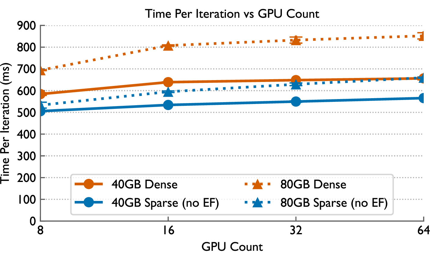
Figure 11 illustrates the time spent in all-reduce and pruning over 80 iterations on 32 GPUs with and without EF. The 80 GB runs spend more time in all-reduce than 40 GB runs, which explains the speedup differences. In both configurations, SpCCL achieves over \(2\times\) speedup on the all-reduce portion. Without EF, pruning introduces \(1.5\) s and \(3\) s of overhead for 40 GB and 80 GB runs, respectively. Pruning time scales linearly with gradient size, as it compares each tensor element against the threshold once and possibly discards them. Since we compute the threshold over a sampled subset of gradients, the sorting cost is minimal.

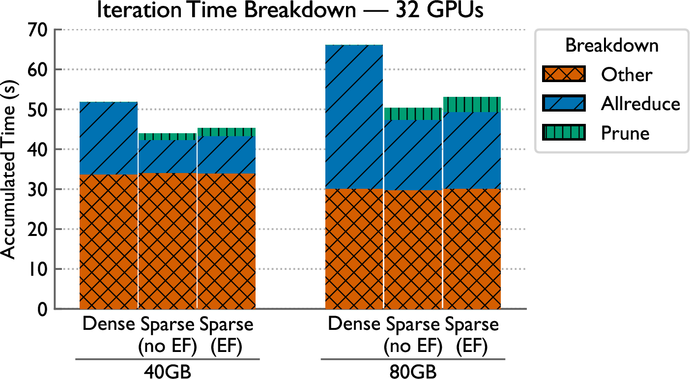
Error feedback introduces overhead in both pruning and all-reduce. In scaling tests, we do not observe EF overhead increasing with GPU count. During pruning, additional error buffer memory traffic accounts for this cost. The source of all-reduce overhead is less apparent. We hypothesize that as error accumulates, the combined error and gradients become more uniform in magnitude during certain iterations. This reduces compression efficiency, degrading all-reduce performance. SpCCL achieves significant speedups with and without EF, demonstrating that sparse collectives can effectively accelerate gradient synchronization in distributed training.

8 Related Work↩︎

Although some prior work explores sparse communication collectives, there are few works that develop exact implementations of collectives designed to work with arbitrary sparse data (particularly outside of all-reduce). SparCML is the work that is conceptually most similar to SpCCL. It supports multiple sparse all-reduce implementations, but operates on host buffers [10]. Unlike SpCCL, it supports only a COO-style representation of sparse data. OmniReduce implements sparse all-reduce as a streaming aggregation system using a block-based sparse representation. Their microbenchmarks apply block-wise sparsity rather than element-wise sparsity, which is very favorable to their approach [[11]][41]. Wijerathne et al. describe block-based collectives implemented in RCCL (and thus exclusive to AMD GPUs), and demonstrate speedups on block-wise sparse inputs [42].

OmNICCL implements sparse all-reduce, but relies on BlueField-2 SmartNICs for in-network aggregation [43]. D-DOSA similarly relies on DPUs/SmartNICs [44].

Several works implement lossy sparse collectives, introducing sparsity during the course of the collective. This may be tolerable for some applications, but lossy collectives are out of scope for this work: SpCCL collectives are exact. Ok-Topk and gTopKAllReduce exemplify this line of research [45], [46].

Hecate implements sparse collectives, but they are sparse in their communication pattern (which ranks participate) rather than in the data communicated [47]. Hoefler et al. also describe collectives that are sparse in their communication pattern [48].

Coruscant introduces a tile- and bitvector-based sparse matrix representation that is similar to Pici [9]. However, the authors design it for use in SpMM kernels rather than for communication. It uses one index per 64-element column in a tile, resulting in \(50\%\) index space overhead relative to the bitvector, compared to Pici’s \(\approx0.78\%\). Additionally, it implements decompression in CUDA only at the tile level, and lacks whole-input (de)compression CUDA kernels.

Our sparse collectives are exact with respect to their inputs. Thus, specific strategies for gradient pruning such as Deep Gradient Compression or \(\text{Gaussian}_k\) are orthogonal to our work [[6]][49]. Such methods may benefit from our work, so long as they don’t require additional sparsification during collectives or alter communication schedules.

9 Conclusion↩︎

In this work, we introduce improvements for the collective communication of sparse data in all-gather, all-reduce, and reduce-scatter, across a range of sparsities. By way of our sparse format, Pici, we reduce the space overhead of communicating moderately sparse data without making assumptions about sparsity structure. Optimized Pici kernels enable efficient (de)compression. Through our phase- and topology-aware adaptive algorithm, we ensure that (de)compression overhead is avoided when it cannot be offset by speedups from sending less data. By implementing SpCCL as an extension to NCCLX, we build our collectives library on a highly optimized foundation, and we highlight the integration and optimization decisions needed to do this well. We demonstrate substantial speedups over sparse and dense baselines: up to \(5.25\times\) for all-gather, \(2.5\times\) for reduce-scatter, and \(2.66\times\) for all-reduce over NCCL at 99% sparsity. These gains translate to end-to-end performance improvements of up to 26% in training gradient-pruned 1.5B and 3.3B LLMs on Perlmutter, emphasizing the utility of our approach in a representative application.

Acknowledgments↩︎

This research used resources of the National Energy Research Scientific Computing Center (NERSC), a Department of Energy User Facility (project m5083). We would also like to thank Siddharth Singh, Prajwal Singhania, and Ashley Adames Perez for valuable advice and feedback on this work.

References↩︎