GlaKG: A Biomarker-Centric Fundus Knowledge Graph for Explainable Glaucoma Diagnosis and Risk Assessment
July 06, 2026
Abstract
Glaucoma is a leading cause of irreversible blindness worldwide, yet most automated diagnosis systems rely on opaque deep-learning models that offer little clinical interpretability. We present GlaKG, a biomarker-centric fundus knowledge graph that integrates structural biomarkers, clinically grounded rules, and image features to produce traceable reasoning for glaucoma diagnosis and risk stratification. GlaKG encodes six entity types (Fundus Image, Optic Disc, Neural Rim, Pathology, Diagnosis, Risk Level), eight relation types, and 11 clinically validated rules into a unified graph, so that every prediction is accompanied by an explicit reasoning chain linking biomarker evidence to activated clinical rules. To keep knowledge-based reasoning strictly separate from label information, we adopt a post-processing fusion framework that combines ResNet50 image embeddings with a normalized KG reasoning-chain score via a tunable weight \(\alpha\), with all fitting confined to the training split. On a publicly available, AI-annotated fundus dataset, GlaKG reaches F1 = 0.9953 for binary glaucoma classification and 0.930 accuracy with 0.922 weighted F1 for four-class risk stratification; we report openly that the dataset’s biomarker annotations are highly label-correlated, and therefore frame these figures as an upper bound attainable with clean structured biomarkers rather than as leakage-free image-only performance. Feature-importance analysis shows KG-derived and biomarker features contributing near-equally (51.1% vs. 48.9%), and the reasoning chain flags borderline cases by exposing low chain scores rather than failing silently. GlaKG’s central contribution is therefore a clinically auditable reasoning framework that complements raw predictive performance by explicitly exposing the biomarker evidence and rule activations behind each decision.
Glaucoma Diagnosis, Knowledge Graph, Explainable AI, Risk Stratification, Graph Neural Network
1 Introduction↩︎
Glaucoma affects over 76 million people worldwide and is projected to reach 111.8 million by 2040 [1]. Early detection is critical, as structural damage to the optic nerve is irreversible. While deep learning approaches have achieved high accuracy in fundus image analysis [2], [3], they suffer from a fundamental limitation: their decision processes are opaque, making it difficult for clinicians to trust or verify automated diagnoses.
Knowledge graphs (KGs) have emerged as a promising paradigm for representing structured medical knowledge, enabling interpretable reasoning over clinical entities and their relationships [4], [5]. However, existing ophthalmic AI systems rarely incorporate structured clinical knowledge such as the ISNT rule, cup-to-disc ratio (CDR) thresholds, or pathological signs like bayoneting and notching. These biomarkers are well-established in clinical practice but are seldom explicitly encoded in automated systems.
In this paper, we present the GlaKG, a biomarker-centric fundus knowledge graph that addresses the lack of structured clinical knowledge integration and interpretable reasoning in existing glaucoma AI systems. Our main contributions are:
A fundus knowledge graph encoding 6 node types, 8 relation types, and 11 clinically validated rules grounded in established ophthalmic guidelines, with any data-informed thresholds fit on the training split only.
A post-processing framework combining ResNet50 visual features with KG reasoning chain scores via a tunable weight \(\alpha\), achieving strong performance on this dataset without end-to-end retraining.
Comprehensive experiments on binary glaucoma classification and four-class risk stratification, with ablation studies, GNN comparisons, feature importance analysis, and error analysis, each accompanied by an interpretable reasoning chain grounded in clinical rules.
2 Related Work↩︎
2.1 Automated Glaucoma Detection & Knowledge Graph↩︎
Convolutional neural networks have demonstrated strong performance in glaucoma detection from ophthalmic photographs [2], [6]–[8], with methods such as GlaBoost [9] further improving accuracy via multimodal biomarker integration and biomarker relationship mining. Recent surveys confirm that deep learning systems analyzing fundus photographs routinely achieve specialist-level sensitivity and specificity [3], [10], yet systematic reviews also highlight persistent challenges in interpretability and clinical deployment [11], [12]. However, these approaches lack explicit clinical knowledge and provide limited interpretability. Knowledge graphs have been successfully applied in drug discovery [13], clinical decision support [14], and disease ontology construction [15], yet structured KGs for glaucoma with explicit biomarker encoding remain underexplored.
2.2 Graph Neural Network & Explainable AI in Healthcare↩︎
GNNs have shown promise in protein interaction networks [16], [17] and electronic health record analysis [5]. Recent work has further demonstrated GNN effectiveness in detecting glaucomatous visual field defects [18], underscoring the potential of graph-structured representations for ophthalmic biomarker analysis. Graph attention networks (GAT) [19] extend GCNs [20] with node-level attention, enabling heterogeneous feature weighting suitable for multi-biomarker clinical graphs. Existing XAI methods for ophthalmic AI primarily rely on gradient-based saliency maps [21], providing pixel-level but not clinical-concept-level explanations, a limitation increasingly recognized in recent XAI surveys [22]. GlaKG addresses this gap via reasoning chains grounded in established clinical criteria.
3 Methodology↩︎
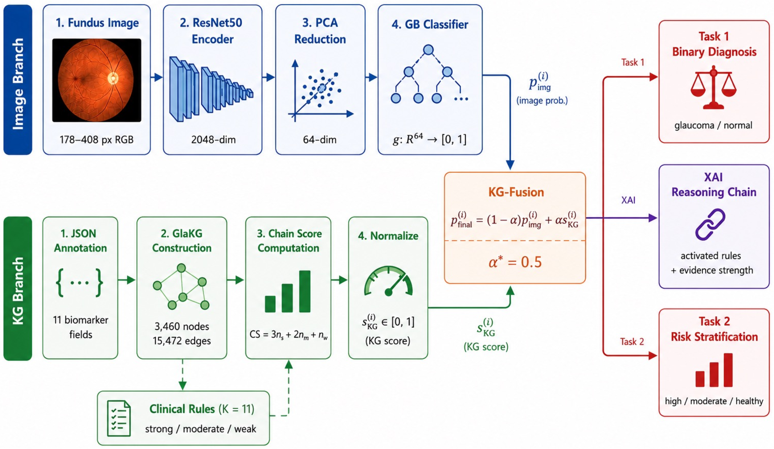
Fig. 1 illustrates the end-to-end GlaKG framework, comprising an image branch, a KG branch, and a post-processing fusion module. The image branch extracts visual features via ResNet50 [23] and produces a glaucoma probability \(p_{\text{img}}^{(i)}\), while the KG branch parses structured biomarker annotations into a heterogeneous graph and computes a normalized reasoning chain score \(s_{\text{KG}}^{(i)}\). The two branches are fused at inference time via Eq. 12 to produce the final prediction.
3.1 GlaKG Construction↩︎
3.1.1 Formal Graph Definition↩︎
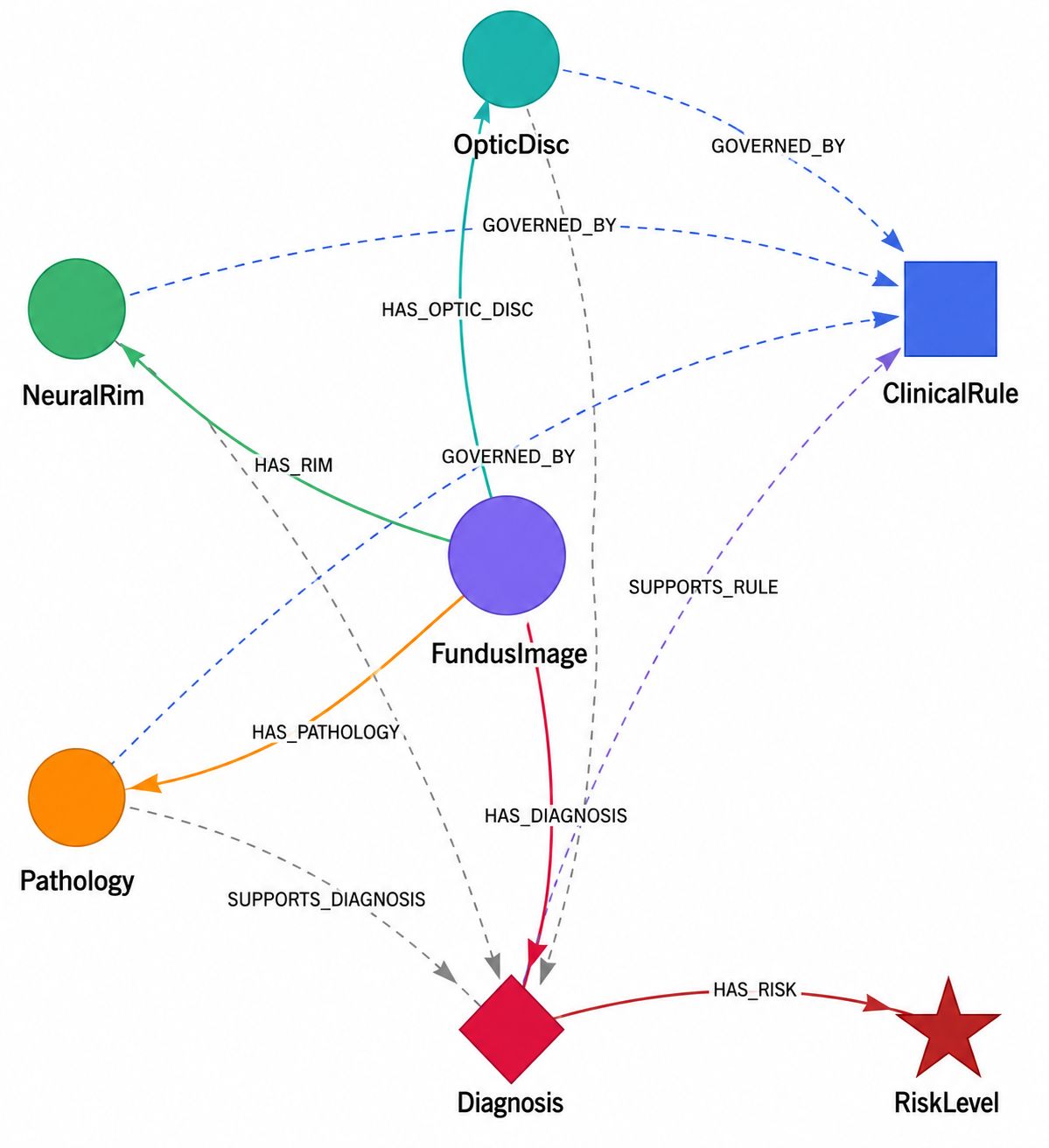
As shown in Fig. 2, GlaKG consists of six entity types connected by eight directed relation types, organized into structural and inference edge categories. We formally define GlaKG as a typed, directed, attributed heterogeneous graph: \[\mathcal{G} = (\mathcal{V}, \mathcal{E}, \mathcal{T}_v, \mathcal{T}_e, \mathcal{X}, \phi, \psi) \label{eq:kg}\tag{1}\] where \(\mathcal{V}\) is the node set, \(\mathcal{E} \subseteq \mathcal{V} \times \mathcal{V}\) is the directed edge set, \(\mathcal{T}_v = \{\)FundusImage, OpticDisc, NeuralRim, Pathology, Diagnosis, RiskLevel\(\}\) is the node type set with \(|\mathcal{T}_v| = 6\), \(\mathcal{T}_e\) is the edge relation type set with \(|\mathcal{T}_e| = 8\), \(\mathcal{X}: \mathcal{V} \rightarrow \mathbb{R}^d\) is the node feature mapping, \(\phi: \mathcal{V} \rightarrow \mathcal{T}_v\) is the node type function, and \(\psi: \mathcal{E} \rightarrow \mathcal{T}_e\) is the edge type function. ClinicalRule nodes serve as auxiliary rule anchors used to materialize supports_rule edges and are not counted among the six entity types in \(\mathcal{T}_v\); including the 11 rule nodes accounts for the total node count reported in Table 7.
The node set is partitioned by type: \[\mathcal{V} = \bigcup_{t \in \mathcal{T}_v} \mathcal{V}_t, \quad \mathcal{V}_i \cap \mathcal{V}_j = \emptyset \;\forall\, i \neq j \label{eq:partition}\tag{2}\]
The edge set is partitioned into structural edges \(\mathcal{E}_s\) and inference edges \(\mathcal{E}_i\): \[\mathcal{E} = \mathcal{E}_s \cup \mathcal{E}_i, \quad \mathcal{E}_s \cap \mathcal{E}_i = \emptyset \label{eq:edges}\tag{3}\] where \(\mathcal{E}_s\) encodes factual associations (has_optic_disc, has_rim, has_pathology, has_diagnosis, has_risk) and \(\mathcal{E}_i\) encodes reasoning relationships (supports_diagnosis, governed_by, supports_rule).
3.1.2 Node Feature Mapping↩︎
Each node \(v \in \mathcal{V}\) is associated with a feature vector \(\mathbf{x}_v \in \mathbb{R}^{d_{\phi(v)}}\), where \(d_{\phi(v)}\) depends on node type. For FundusImage nodes, features are extracted via a pretrained ResNet50 encoder \(f_\theta: \mathbb{R}^{H \times W \times 3} \rightarrow \mathbb{R}^{2048}\), subsequently projected to \(\mathbb{R}^{64}\) via PCA: \[\mathbf{x}_v^{img} = \mathbf{P}^\top f_\theta(I_v) \in \mathbb{R}^{64}, \quad \mathbf{P} \in \mathbb{R}^{2048 \times 64} \label{eq:pca}\tag{4}\] For biomarker nodes, features are structured attribute vectors derived from clinical annotations: \[\mathbf{x}_v = [a_1^{(v)}, \ldots, a_{d_{\phi(v)}}^{(v)}]^\top \in \mathbb{R}^{d_{\phi(v)}} \label{eq:biofeature}\tag{5}\] where \(a_j^{(v)} \in \{0,1\}\) for boolean attributes and \(a_j^{(v)} \in \mathbb{R}\) for continuous attributes (e.g., CDR). All node features are zero-padded to a unified dimension \(d = 64\) for GNN processing.
3.2 Clinical Rule Encoding↩︎
3.2.1 Rule Formalization↩︎
We define a set of \(K{=}11\) clinical rules \(\mathcal{R} = \{r_1, \ldots, r_K\}\), where each rule is a 4-tuple: \[r_k = (b_k,\;\bowtie_k,\;\tau_k,\;s_k) \label{eq:rule}\tag{6}\] with \(b_k\) the target biomarker attribute, \(\bowtie_k \in \{\geq, \leq, =\}\) the comparison operator, \(\tau_k\) the threshold value, and \(s_k \in \{1, 2, 3\}\) the strength weight (weak [24], moderate [25], strong [26], [27] respectively).
3.2.2 Rule Activation↩︎
For a diagnosis node \(v_{diag}\) associated with biomarker node \(v_b\), rule \(r_k\) is activated if and only if: \[\mathbb{1}[r_k, v_b] = \begin{cases} 1 & \text{if } a_{b_k}^{(v_b)} \bowtie_k \tau_k \\ 0 & \text{otherwise} \end{cases} \label{eq:activation}\tag{7}\] The activated rule set for a diagnosis node is: \[\mathcal{R}(v_{diag}) = \{r_k \in \mathcal{R} : \mathbb{1}[r_k, v_b] = 1\} \label{eq:activated95set}\tag{8}\] A supports_rule edge \((v_{diag}, r_k)\) is created for each \(r_k \in \mathcal{R}(v_{diag})\), forming the explicit reasoning chain.
3.2.3 Reasoning Chain Score↩︎
The reasoning chain score aggregates weighted rule activations: \[\text{CS}(v_{diag}) = \sum_{k=1}^{K} s_k \cdot \mathbb{1}[r_k, v_b] = 3\,n_{\text{strong}} + 2\,n_{\text{moderate}} + n_{\text{weak}} \label{eq:chain}\tag{9}\] where \(n_{\text{strong}} = |\{r_k \in \mathcal{R}(v_{diag}): s_k = 3\}|\), and \(n_{\text{moderate}}\), \(n_{\text{weak}}\) are defined analogously. The maximum achievable score is \(\text{CS}_{\max} = 3 \times 3 + 2 \times 4 + 1 = 18\). This maximum reflects the largest mutually compatible rule subset (3 strong, 4 moderate, 1 weak): several rules are mutually exclusive (e.g., \(\text{CDR} \geq 0.7\) and \(\text{CDR} < 0.4\) cannot co-activate), so the attainable maximum of 8 co-activated rules is below the total \(K = 11\).
3.3 KG-Fusion Inference Framework↩︎
To avoid data leakage between KG-derived features and classification labels, we adopt a post-processing fusion strategy operating entirely at inference time.
3.3.1 Image-Based Probability↩︎
Let \(\mathbf{z}_i = \mathbf{P}^\top f_\theta(I_i) \in \mathbb{R}^{64}\) denote the PCA-projected image embedding for sample \(i\). A Gradient Boosting classifier \(g: \mathbb{R}^{64} \rightarrow [0,1]\) is trained to produce: \[p_{\text{img}}^{(i)} = g(\mathbf{z}_i) \in [0,1] \label{eq:pimg}\tag{10}\] where \(p_{\text{img}}^{(i)}\) represents the probability of glaucoma from visual features alone.
3.3.2 KG Reasoning Score Normalization↩︎
The raw chain score \(\text{CS}(v_{diag}^{(i)})\) is min-max normalized across the dataset \(\mathcal{D}\): \[s_{\text{KG}}^{(i)} = \frac{\text{CS}(v_{diag}^{(i)}) - \min_{j \in \mathcal{D}} \text{CS}(v_{diag}^{(j)})}{\max_{j \in \mathcal{D}} \text{CS}(v_{diag}^{(j)}) - \min_{j \in \mathcal{D}} \text{CS}(v_{diag}^{(j)}) + \epsilon} \label{eq:norm}\tag{11}\] where \(\epsilon = 10^{-8}\) ensures numerical stability, yielding \(s_{\text{KG}}^{(i)} \in [0,1]\).
3.3.3 Fusion and Prediction↩︎
The final prediction probability is a convex combination of the image-based and KG-based scores: \[p_{\text{final}}^{(i)} = (1 - \alpha)\,p_{\text{img}}^{(i)} + \alpha\,s_{\text{KG}}^{(i)}, \quad \alpha \in [0,1] \label{eq:fusion}\tag{12}\] The predicted label is: \[\hat{y}_i = \mathbb{1}\left[p_{\text{final}}^{(i)} \geq 0.5\right] \label{eq:decision}\tag{13}\] The optimal fusion weight \(\alpha^* = \arg\max_{\alpha} \mathcal{F}_1(\alpha)\) is determined via 5-fold cross-validation over \(\alpha \in \{0.0, 0.3, 0.5, 0.7, 1.0\}\), yielding \(\alpha^* = 0.5\).
3.4 Graph Neural Network Variant↩︎
3.4.1 Per-Case Subgraph Construction↩︎
For each sample \(i\), we extract a local subgraph \(\mathcal{G}^{(i)} \subset \mathcal{G}\) centered on the corresponding FundusImage node: \[\mathcal{G}^{(i)} = \left(\mathcal{V}^{(i)}, \mathcal{E}^{(i)}\right) \label{eq:subgraph}\tag{14}\] where \(\mathcal{V}^{(i)} = \{v_{img}^{(i)}, v_{od}^{(i)}, v_{rim}^{(i)}, v_{path}^{(i)}, v_{diag}^{(i)}\}\) with \(|\mathcal{V}^{(i)}| = 5\), and \(|\mathcal{E}^{(i)}| = 14\) including both forward and reverse edges to support bidirectional message passing. Node features are assembled as: \[\mathbf{X}^{(i)} = \left[\mathbf{x}_{v_1}^{(i)}, \ldots, \mathbf{x}_{v_5}^{(i)}\right]^\top \in \mathbb{R}^{5 \times 64} \label{eq:nodematrix}\tag{15}\]
3.4.2 GCN Message Passing↩︎
The \(l\)-th layer of the GCN updates node representations via: \[\mathbf{h}_v^{(l)} = \sigma\!\left( \mathbf{W}^{(l)} \sum_{u \in \mathcal{N}(v) \cup \{v\}} \frac{\mathbf{h}_u^{(l-1)}}{\sqrt{|\mathcal{N}(v)||\mathcal{N}(u)|}} \right) \label{eq:gcn}\tag{16}\] where \(\mathbf{W}^{(l)} \in \mathbb{R}^{d_{l} \times d_{l-1}}\) is a learnable weight matrix, \(\mathcal{N}(v)\) denotes the neighbor set of \(v\), \(\sigma\) is ReLU activation, and \(\mathbf{h}_v^{(0)} = \mathbf{x}_v\).
3.4.3 GAT Message Passing↩︎
The \(l\)-th layer of the GAT computes multi-head attention: \[\mathbf{h}_v^{(l)} = \Big\|_{m=1}^{M} \sigma\!\left( \sum_{u \in \mathcal{N}(v) \cup \{v\}} \alpha_{vu}^{(m,l)}\, \mathbf{W}_m^{(l)} \mathbf{h}_u^{(l-1)} \right) \label{eq:gat}\tag{17}\] where \(M = 4\) is the number of attention heads, \(\|\) denotes concatenation. Let \(e_{vu}^{(m,l)} = \text{LeakyReLU}\!\left( \mathbf{a}_m^\top [\mathbf{W}_m^{(l)}\mathbf{h}_v^{(l-1)} \| \mathbf{W}_m^{(l)}\mathbf{h}_u^{(l-1)}]\right)\), then the attention coefficient is: \[\alpha_{vu}^{(m,l)} = \frac{\exp(e_{vu}^{(m,l)})}{\sum_{w \in \mathcal{N}(v) \cup \{v\}} \exp(e_{vw}^{(m,l)})} \label{eq:attn}\tag{18}\] with \(\mathbf{a}_m \in \mathbb{R}^{2d_l}\) a learnable attention vector. For the final layer (\(l = L\)), mean aggregation replaces concatenation to obtain a fixed-size output representation: \[\mathbf{h}_v^{(L)} = \sigma\!\left( \frac{1}{M}\sum_{m=1}^{M} \sum_{u \in \mathcal{N}(v) \cup \{v\}} \alpha_{vu}^{(m,L)}\, \mathbf{W}_m^{(L)} \mathbf{h}_u^{(L-1)} \right) \label{eq:gat95final}\tag{19}\]
3.4.4 Graph-Level Prediction↩︎
After \(L = 2\) message-passing layers, a graph-level representation is obtained via global mean pooling: \[\mathbf{h}_{\mathcal{G}^{(i)}} = \frac{1}{|\mathcal{V}^{(i)}|} \sum_{v \in \mathcal{V}^{(i)}} \mathbf{h}_v^{(L)} \in \mathbb{R}^{d_L} \label{eq:pool}\tag{20}\] The final classification is: \[\hat{y}_i = \arg\max_{c \in \{0,1\}} \text{softmax}\!\left( \mathbf{W}_2\,\sigma\!\left( \mathbf{W}_1\,\mathbf{h}_{\mathcal{G}^{(i)}} + \mathbf{b}_1 \right) + \mathbf{b}_2 \right)_c \label{eq:cls}\tag{21}\] where \(\mathbf{W}_1, \mathbf{W}_2, \mathbf{b}_1, \mathbf{b}_2\) are learnable parameters of the two-layer MLP head. Both GCN and GAT are optimized with cross-entropy loss: \[\mathcal{L} = -\frac{1}{N} \sum_{i=1}^{N} \left[y_i \log \hat{p}_i + (1-y_i)\log(1-\hat{p}_i)\right] \label{eq:loss}\tag{22}\] using Adam optimizer with learning rate \(10^{-3}\), weight decay \(10^{-4}\), and batch size 32 for 60 epochs.
4 Dataset & Implementation↩︎
4.1 Dataset↩︎
4.1.1 Data Source↩︎
We use a publicly available fundus dataset [28] with rich structured annotations. Each sample includes a fundus image (178–408 px), binary annotation (glaucoma/normal), and a structured JSON description encoding 11 biomarker fields, risk assessment levels (high risk / moderate risk / healthy / very healthy), and confidence scores.
4.1.2 Dataset Characteristics↩︎
The dataset contains 689 samples with a class imbalance of 63.7% glaucoma and 36.3% normal, motivating F1-score as the primary evaluation metric. CDR values are well-separated between classes (glaucoma: mean = 0.767, \(\sigma\) = 0.072; normal: mean = 0.400, \(\sigma\) = 0.063). Among glaucoma cases, rim thinning and ISNT rule violation are universal (100% prevalence), bayoneting, notching, and rim pallor appear in \(\sim\)73% of cases, and laminar dot sign in 55%. All pathological signs are absent in normal cases (0%); as discussed in Sec. IV-B1, this strong separation reflects the label-correlated nature of the AI-generated annotations. The risk level distribution is: high risk (55.2%), moderate risk (6.7%), healthy (1.2%), and very healthy (36.9%). The original train/test partition yields 551 training and 138 test samples with no leakage across splits.
4.1.3 Pre-Processing Pipeline↩︎
each sample’s structured JSON description is parsed to extract 11 biomarker fields, including cup-to-disc ratio (CDR), ISNT rule compliance, rim thinning, rim pallor, bayoneting, notching, and laminar dot sign. Boolean fields are mapped to binary values \(\{0, 1\}\) and CDR is retained as a continuous variable. The dataset is split into training and test sets following the original partition (train-00000-of-00001 and test-00000-of-00001), with a split ratio of approximately 80%/20%. Fundus images are resized to \(224 \times 224\) pixels, normalized with ImageNet mean and standard deviation, and passed through a pretrained ResNet50 backbone (fc layer replaced by Identity) to extract 2048-dimensional embeddings, which are subsequently reduced to 64 dimensions via PCA for GNN node feature initialization. All continuous features are standardized to zero mean and unit variance prior to classifier training.
4.2 Implementation↩︎
4.2.1 Data Leakage Prevention and Annotation-Label Correlation↩︎
We handle the relationship between the structured description field and the classification annotation on three fronts: strict pipeline hygiene, open reporting of a label-correlated dataset property, and grounding our
contribution in interpretability rather than raw accuracy.
Pipeline hygiene. All fitting is confined to the training split: (i) the 551/138 partition follows the dataset’s original split; (ii) PCA \(\mathbf{P}\) and feature standardization are fit on training embeddings only; (iii) rule thresholds \(\tau_k\) derive from clinical guidelines (e.g., \(\text{CDR}\geq 0.7\)), not labels; (iv) \(\alpha^*\) is chosen by 5-fold CV within the training split, with the test set held out. The KG score \(s_{\text{KG}}^{(i)}\) never enters training: \(g\) sees only ResNet50 embeddings, and \(s_{\text{KG}}^{(i)}\) is fused at inference (Eq. 12 ). This precludes both split leakage and \(s_{\text{KG}}^{(i)}\) acting as a label proxy.
Annotation-label correlation. The biomarker annotations are strongly discriminative: rim thinning and ISNT violation are universal in glaucoma (100%), all pathological signs are absent in normal cases (0%), and the KG-only model ranks the classes near-perfectly (AUC \(=1.000\), Table 3). We state this openly: the annotations, from an independent AI pipeline, are themselves label-correlated on this dataset. The fused \(\text{F1}=0.9953\) is therefore an upper bound achievable with clean structured biomarkers, not a claim of leakage-free image-only performance.
Interpretability is leakage-invariant. GlaKG’s contribution does not depend on the metrics being leakage-free. For every prediction it exposes which rules fired, at what strength, and how they aggregate, a clinician-style audit trail that holds regardless of annotation correlation. The single missed case (CDR \(=0.700\); chain score 9 vs.a correct-case mean of 15.91) shows the chain flagging its own uncertainty on borderline inputs rather than failing silently.
4.2.2 Hyperparameter↩︎
the KG-fusion framework uses Gradient Boosting as the image-based classifier (100 estimators, learning rate = 0.1) trained on 64-dimensional PCA-reduced ResNet50 embeddings. The fusion weight \(\alpha\) is selected from \(\{0.0, 0.3, 0.5, 0.7, 1.0\}\) via cross-validation, with \(\alpha{=}0.5\) achieving optimal performance. For GCN, hidden dimension is set to 128 with dropout 0.3. For GAT, hidden dimension is 64 with 4 attention heads and dropout 0.3. Both GNN models are trained with Adam optimizer (learning rate = 1e-3, weight decay = 1e-4) for 60 epochs with batch size 32. All experiments use random seed 42 for reproducibility.
4.2.3 Hardware↩︎
all experiments were conducted on a server equipped with 4×NVIDIA A100 GPUs (80GB each). Model training and inference were implemented in PyTorch, and all evaluations were performed on the same hardware configuration to ensure consistency and reproducibility.
4.2.4 Evaluation Metrics↩︎
for binary glaucoma classification, we report Accuracy, Precision, Recall, F1-score, and Area Under the ROC Curve (AUC). F1-score is the primary metric given the class imbalance (glaucoma: 63.7%, normal: 36.3%). For four-class risk stratification, we additionally report macro-averaged F1 (F1mac) and weighted F1 (F1wt) to account for label imbalance across risk levels. All metrics are reported as the mean over 5-fold stratified cross-validation folds; per-fold variance is small, indicating that the reported results are stable across splits rather than an artifact of a single favorable partition. For knowledge graph quality assessment, we report four structural metrics. Graph density measures the ratio of actual edges to all possible edges, reflecting graph sparsity. Largest connected component (LCC) ratio measures the proportion of nodes in the largest weakly connected component, indicating overall graph connectivity. Average rules per diagnosis quantifies the mean number of activated clinical rules per case, reflecting reasoning chain richness. Rule coverage reports the percentage of diagnoses activated by at least \(k\) rules (\(k \in \{1, 3\}\)), measuring the completeness of clinical knowledge encoding. Additionally, KG feature contribution is measured via Mean Decrease in Impurity (MDI) feature importance, quantifying the relative decision-making weight of KG-derived versus biomarker features.
5 Experimental Result↩︎
5.1 Experimental Setup↩︎
5.1.1 Baseline Model↩︎
we evaluate four image-only baselines to assess the contribution of KG reasoning chains. Logistic Regression (LR) [29] serves as a linear baseline with \(\ell_2\) regularization (max_iter = 1000). Random Forest (RF) [30] uses 200 estimators with default hyperparameters. Gradient Boosting (GB) uses 100 estimators and serves as the backbone classifier for our KG-fusion framework. Multilayer Perceptron (MLP) [31] consists of two hidden layers (256, 64) with ReLU activation and 500 training epochs. All baselines operate exclusively on ResNet50 [23] image embeddings and are evaluated under identical 5-fold stratified cross-validation (seed = 42). For GNN baselines, we evaluate GCN [20] and GAT [19] operating on per-case KG subgraphs with unified 64-dimensional node features.
5.1.2 Task Definition↩︎
We evaluate GlaKG on two classification tasks:
Task 1: Binary Glaucoma Classification Given a fundus image and its associated KG subgraph, the model predicts whether the sample belongs to the glaucoma or normal class. This is a standard binary classification task with class imbalance (glaucoma: 63.7%, normal: 36.3%).
Task 2: Four-class Risk Stratification Given the same inputs, the model predicts one of four risk levels: high risk, moderate risk, healthy, or very healthy. This task is more fine-grained than binary classification and evaluates the model’s ability to distinguish adjacent risk levels that may share similar visual appearances.
5.2 Comparative Experiment↩︎
Table 1 presents the binary glaucoma classification results across all methods. Image-only baselines achieve F1 scores in the range of 0.903–0.909 and AUC in the range of 0.942–0.949, reflecting the inherent difficulty of distinguishing glaucomatous cases from visual features alone. GCN improves over the best image-only baseline by 1.2 and 1.5 percentage points in F1 and AUC, confirming that graph-structured biomarker representations provide complementary information beyond raw image embeddings. GAT further improves over GCN by 5.3 and 2.7 percentage points in F1 and AUC, demonstrating that attention-based aggregation effectively captures the heterogeneous diagnostic importance of different biomarker nodes. Our KG-fusion method achieves the highest overall performance with F1 = 0.9953 and AUC = 0.9988, outperforming the best image-only baseline by 8.3 and 5.0 percentage points in F1 and AUC, respectively.
| Method | Acc | Prec | Rec | F1 | AUC |
|---|---|---|---|---|---|
| B1 LR (img) | 0.8854 | 0.8945 | 0.9250 | 0.9094 | 0.9417 |
| B2 RF (img) | 0.8723 | 0.8388 | 0.9836 | 0.9053 | 0.9423 |
| B3 GB (img) | 0.8869 | 0.8771 | 0.9509 | 0.9124 | 0.9487 |
| B4 MLP (img) | 0.8767 | 0.8811 | 0.9274 | 0.9029 | 0.9417 |
| GCN | 0.9072 | 0.9277 | 0.9227 | 0.9247 | 0.9641 |
| GAT | 0.9710 | 0.9555 | 1.0000 | 0.9772 | 0.9912 |
| Ours (\(\alpha\)=0.5) | 0.9942 | 1.0000 | 0.9906 | 0.9953 | 0.9988 |
For four-class risk stratification (Table 2), image-only baselines achieve weighted F1 in the range of 0.781–0.823, with macro F1 substantially lower (0.475–0.537), indicating difficulty in distinguishing minority risk levels. Our method achieves accuracy of 0.930 and weighted F1 of 0.922, outperforming all baselines by at least 9.8 and 9.9 percentage points in accuracy and weighted F1, respectively. We note that the four-class AUC does not exceed the strongest image-only baseline, consistent with AUC being less sensitive to the minority-class gains that KG reasoning chains provide. The improvement in accuracy and weighted F1 is more pronounced for risk stratification than binary classification, suggesting that KG reasoning chains provide particularly strong evidence for distinguishing adjacent risk levels that are visually ambiguous.
| Method | Acc | F1mac | F1wt | AUC |
|---|---|---|---|---|
| B1 LR (img) | 0.8316 | 0.5343 | 0.8230 | 0.7752 |
| B2 RF (img) | 0.8012 | 0.4746 | 0.7802 | 0.8382 |
| B3 GB (img) | 0.8273 | 0.5343 | 0.8205 | 0.7774 |
| B4 MLP (img) | 0.8186 | 0.5370 | 0.8110 | 0.8286 |
| Ours (\(\alpha\)=0.5) | 0.9303 | 0.6127 | 0.9222 | 0.8010 |
5.3 Ablation Study↩︎
We conduct two groups of ablation experiments to evaluate the contribution of individual components in GlaKG.
5.3.1 KG Fusion Weight (Binary Classification)↩︎
Table 3 reports the effect of varying \(\alpha\) on binary classification. When \(\alpha{=}0\) (image only), the model achieves F1 = 0.9124 and AUC = 0.9466. Introducing KG reasoning chain scores progressively improves performance, peaking at F1 = 0.9953 and AUC = 0.9988 at \(\alpha{=}0.5\). Beyond this point, performance degrades as the KG signal dominates, confirming that visual features and KG reasoning chains are complementary and neither is sufficient in isolation.
At \(\alpha=1.0\), the KG score ranks cases near-perfectly (AUC \(=1.000\)) yet F1 drops to 0.8412: with a fixed 0.5 decision threshold, precision is 1.000 but recall falls to 0.726, i.e., the ranking is separable but the operating point is conservative. This confirms that the KG signal’s separating power derives from label-correlated biomarkers (Sec. IV-B1), which is precisely why fusion with independent visual features, rather than the KG alone, is necessary for a calibrated decision.
| \(\alpha\) | Acc | Prec | Rec | F1 | AUC |
|---|---|---|---|---|---|
| 0.0 | 0.8868 | 0.8769 | 0.9508 | 0.9124 | 0.9466 |
| 0.3 | 0.9318 | 0.9222 | 0.9719 | 0.9464 | 0.9896 |
| 0.5 | 0.9942 | 1.0000 | 0.9906 | 0.9953 | 0.9988 |
| 0.7 | 0.9797 | 1.0000 | 0.9672 | 0.9833 | 0.9999 |
| 1.0 | 0.8302 | 1.0000 | 0.7260 | 0.8412 | 1.0000 |
5.3.2 KG Fusion Weight (Risk Stratification)↩︎
Table 4 presents the ablation for risk stratification. Accuracy, macro-F1, and weighted-F1 all peak at \(\alpha{=}0.5\) (0.9303 / 0.6127 / 0.9222), consistent with the binary-classification optimum, while AUC peaks earlier at \(\alpha{=}0.3\) (0.8679). Performance degrades as \(\alpha \rightarrow 1.0\), confirming that visual and KG signals are complementary for risk stratification as well.
| \(\alpha\) | Acc | F1mac | F1wt | AUC |
|---|---|---|---|---|
| 0.0 | 0.8273 | 0.5360 | 0.8213 | 0.7793 |
| 0.3 | 0.8476 | 0.5487 | 0.8409 | 0.8679 |
| 0.5 | 0.9303 | 0.6127 | 0.9222 | 0.8010 |
| 0.7 | 0.9173 | 0.5435 | 0.8960 | 0.8429 |
| 1.0 | 0.8200 | 0.4254 | 0.7939 | 0.8085 |
5.4 Analysis↩︎
5.4.1 Explainability↩︎
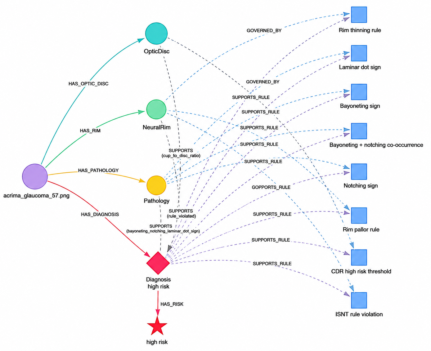
Fig. 3 visualizes the reasoning chain for a representative high-risk glaucoma case, tracing diagnostic evidence from biomarker nodes to activated clinical rules via supports_rule edges. The case
activates 6 rules including all 3 strong rules (CDR threshold, rim thinning, ISNT violation), yielding a chain score of 15 (3 strong plus 3 moderate rules), well above the single false negative case (chain score: 9). Feature importance analysis (MDI)
reveals that KG features contribute 51.1% of model decisions, with n_rules (0.3352) and chain_score (0.1565) ranking 1st and 3rd among all features, as shown in Fig. 4.
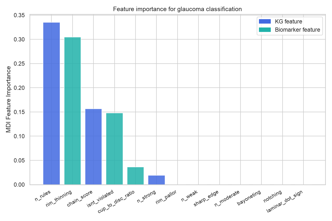
Biomarker features contribute 48.9%, with rim_thinning (0.3047) and isnt_violated (0.1478) ranking 2nd and 4th (Table 5). This near-equal contribution confirms the complementary nature of structured
knowledge and visual biomarkers.
| Rank | Feature | Type | Importance |
|---|---|---|---|
| 1 | n_rules | KG | 0.3352 |
| 2 | rim_thinning | Biomarker | 0.3047 |
| 3 | chain_score | KG | 0.1565 |
| 4 | isnt_violated | Biomarker | 0.1478 |
| 5 | cup_to_disc_ratio | Biomarker | 0.0365 |
5.4.2 Error Analysis↩︎
Table 6 summarizes prediction outcomes on the test set (\(n{=}138\)). Our method achieves zero false positives and only one false negative (FN rate = 0.7%), corresponding to an overall accuracy of 99.3%. The single missed case exhibits CDR = 0.700, precisely at the clinical threshold, and activates only 3 rules compared to a mean of 6.39 for correctly classified cases (chain score: 9 vs.). This indicates that the primary failure mode is borderline cases where both visual and KG evidence are simultaneously weak.
| Type | Count | Rate |
|---|---|---|
| True Positive (TP) | 85 | 61.6% |
| True Negative (TN) | 52 | 37.7% |
| False Positive (FP) | 0 | 0.0% |
| False Negative (FN) | 1 | 0.7% |
| FN: Avg CDR | 0.700 (TP: 0.767) | |
| FN: Avg chain score | 9.00 (TP: 15.91) | |
| FN: Avg \(n_{\text{rules}}\) | 3.00 (TP: 6.39) | |
5.4.3 Knowledge Graph Quality↩︎
Table 7 reports structural and coverage metrics. The LCC ratio of 1.000 confirms full graph connectivity. Glaucoma cases activate an average of 3.69 strong rules vs. for normal cases, validating the discriminative power of the encoded clinical knowledge. KG feature contribution of 51.1% confirms that encoded rules provide non-redundant signals beyond raw biomarker features.
| Metric | Value |
|---|---|
| Total nodes | 3,460 |
| Total edges | 15,472 |
| Node / edge types | 6 / 8 |
| Clinical rules | 11 |
| Graph density | \(1.23 \times 10^{-3}\) |
| Largest CC ratio | 1.000 |
| Avg degree | 8.94 |
| Avg rules per diagnosis | 4.36 |
| Avg chain score | 11.04 |
| Covered (\(\geq\)1 rule) | 689/689 (100.0%) |
| Covered (\(\geq\)3 rules) | 427/689 (62.0%) |
| Avg strong rules (glaucoma) | 3.69 |
| Avg strong rules (normal) | 1.00 |
| KG feature contribution | 51.1% |
5.5 Clinical Implications↩︎
GlaKG offers several clinically meaningful advantages over conventional deep learning approaches for glaucoma screening.
5.5.1 Interpretable Reasoning Chains↩︎
unlike black-box CNN models, GlaKG provides an explicit reasoning chain for every diagnosis, listing activated clinical rules with their evidence strength. For example, a severe high-risk case that activates the full set of eight mutually compatible rules attains the maximum chain score of 18, giving clinicians a structured audit trail that mirrors their own diagnostic reasoning process.
5.5.2 Alignment with Clinical Guidelines↩︎
the 11 encoded rules are grounded in established ophthalmic guidelines, including the ISNT rule and the CDR \(\geq\) 0.7 threshold recommended by the International Council of Ophthalmology. This alignment ensures that GlaKG’s reasoning chains are immediately interpretable to ophthalmologists without additional training.
5.5.3 Failure Mode Transparency↩︎
the single false negative case (CDR = 0.700, chain score = 9) demonstrates that GlaKG’s reasoning chain explicitly signals diagnostic uncertainty: a low chain score flags borderline cases for clinician review rather than producing a silent misclassification. This property is clinically critical, as missed glaucoma diagnoses carry higher risk than false positives.
5.5.4 Integration Potential↩︎
GlaKG’s modular design separates image-based inference from knowledge-based reasoning, allowing either component to be updated independently. New clinical biomarkers (e.g., RNFL thickness, visual field indices) can be incorporated as additional ClinicalRule nodes without retraining the image encoder, facilitating seamless integration into existing ophthalmic AI workflows.
6 Conclusion↩︎
In this paper, we presented GlaKG, a biomarker-centric fundus knowledge graph for explainable glaucoma diagnosis and risk assessment. GlaKG encodes 6 entity types, 8 relation types, and 11 clinically validated rules into a unified graph structure, so that every prediction is accompanied by an explicit reasoning chain linking biomarker evidence to activated clinical rules. On a publicly available, AI-annotated fundus dataset, the proposed post-processing fusion framework attains F1 = 0.9953 for binary glaucoma classification and 0.930 accuracy with 0.922 weighted F1 for four-class risk stratification, surpassing image-only baselines in accuracy and weighted F1. We report openly that the dataset’s biomarker annotations are highly label-correlated, and therefore frame these figures as an upper bound attainable with clean structured biomarkers rather than as leakage-free image-only performance; the value of GlaKG lies not solely in raw performance metrics but in a clinically auditable reasoning chain that exposes its own uncertainty on borderline cases. Feature-importance analysis further shows KG-derived and biomarker features contributing near-equally (51.1% vs.%), confirming their complementarity. GlaKG establishes a foundation for trustworthy, clinically interpretable glaucoma screening systems.
7 Limitation & Future Work↩︎
GlaKG has several limitations. First, it relies on structured JSON annotations for biomarker extraction, which may limit real-world deployment. Future work will explore automatic biomarker extraction from raw fundus images through joint image-KG learning. Second, the current graph is static and does not capture disease progression over time. Incorporating longitudinal biomarkers and temporal edges may enable progression modeling and early intervention prediction. Third, its generalizability across fundus datasets and imaging devices requires further validation through cross-dataset evaluation and domain adaptation. Finally, extending GlaKG to other ophthalmic diseases, such as diabetic retinopathy and age-related macular degeneration, may broaden its clinical applicability.
Acknowledgment↩︎
This work is supported in part by the Cancer Prevention and Research Institute of Texas (CPRIT) under Grant RP250561.