Attention Limited Reward Learning
July 06, 2026
Abstract
Pairwise human comparisons are a primary interface through which modern AI systems learn human preferences. RLHF and related alignment pipelines typically model such comparisons with Bradley–Terry log-odds, where choice probabilities are governed by latent reward differences. This paper examines what this assumption misses through a reduced-form model motivated by rational inattention, in which each label is generated by a low-capacity evaluation channel. The model separates two forms of ambiguity that standard reward modeling tends to conflate: a comparison may be difficult because the two candidates are genuinely close in value, or because the relevant distinction is hard to detect under limited attention. We show that limited attention can fundamentally distort what pairwise comparisons reveal. In particular, passive comparison data cannot generally distinguish reward, attention, and default tendencies, and heterogeneous attention can make standard Bradley–Terry reward modeling recover misleading rankings. Our analysis shows that learning is governed not by the raw number of labels, but by the amount of attended information each label carries. A case study on human votes over language-model pairs from Chatbot Arena exhibits the predicted signature, a cyclic component of the comparison data that exceeds sampling noise and that no scalar reward can represent; a second case study on perceptual comparisons shows that response times and gaze carry gap information that the labels do not. This perspective suggests that human feedback should be treated not as direct revealed preference, but as an attention-limited measurement process: a weak preference signal may reflect hidden evaluation difficulty rather than genuine indifference.
1 Introduction↩︎
Human feedback has become a central part of how modern AI systems are trained and evaluated. In reinforcement learning from human feedback (RLHF), preference-based policy optimization, and related alignment pipelines, the basic measurement primitive is often simple. A human is shown two candidate responses, rankings, plans, allocations, or trajectories and asked which one is better. A reward model is then trained so that its pairwise differences predict these choices. This template underlies much of contemporary reward learning for language models and agentic systems [1]–[5]. Direct preference optimization changes the downstream policy update, but it still relies on the same basic comparison signal linking human choices to reward differences [6].
The standard statistical abstraction is the Bradley–Terry, or conditional-logit, model [7]–[9]. For a query consisting of a context \(x\) and two candidates \(y^0,y^1\), it assumes \[\mathbb{P}[y^1 \succ y^0\mid x] = \sigma\bigl(r(x,y^1)-r(x,y^0)\bigr), \qquad \sigma(t)=\frac{1}{1+e^{-t}} . \label{eq:bt-intro}\tag{1}\] Under this model, comparison labels are noisy but direct measurements of a single latent reward. If two candidates are chosen at roughly equal rates, the model interprets this as evidence that their rewards are nearly equal. Much of the statistical ranking literature studies estimation and ranking in this correctly specified regime [10], [11].
For alignment, however, the most important comparisons are often not the easiest ones. A response may be fluent but subtly misleading. A plan may appear helpful while creating long-run risks. A model output may satisfy the literal request while violating the user’s underlying intent. In such cases, the relevant distinction is not necessarily small; it may simply be hard to notice. This observation is the premise of work on scalable oversight, which anticipates that as systems become more capable, the outputs whose evaluation matters most are the ones that strain unaided human judgment [12]–[15]. Human evaluators operate with limited time, limited context, and limited cognitive bandwidth. They attend to surface features that are cheap to check, such as fluency, length, format, and confidence, and can miss properties that require costly deliberation, a pattern documented empirically in reward models that absorb such surface regularities [16], [17]. This is not just random noise around a fixed reward. It is a structured measurement problem.
We model this problem using an attention-scaled reduced form motivated by rational inattention. A rationally inattentive evaluator allocates scarce information-processing effort before making a choice [18]–[21]. Some comparisons are cheap to evaluate because one answer is incoherent, one plan obviously fails, or one candidate plainly violates an instruction. Others require careful reasoning about factual dependencies, safety implications, long-horizon consequences, or subtle forms of misalignment. A Shannon rational-inattention first-order condition, derived in Section 2, motivates a marginal comparison channel of the form \[\ell_z=\eta_z+\beta_z\Delta_z^*, \label{eq:intro-channel}\tag{2}\] where \(\Delta_z^*\) is the deliberative reward difference for query \(z\), \(\beta_z\ge0\) is an attention multiplier, and \(\eta_z\) is a default, order, prior, or salience term. Thus the observed label is not just a noisy draw from the reward difference. It is the output of an attention-limited channel whose strength varies across queries.
This channel highlights a distinction that is central to alignment. A comparison can be hard because close, in that the two candidates genuinely have similar deliberative value. A comparison can also be hard because hidden, in that the reward-relevant difference is large but the evidence needed to see it is costly or non-salient, so the observed choice probability remains near \(50\)–\(50\). Standard Bradley–Terry modeling treats both cases as small reward gaps. For alignment this conflation is dangerous, because the hard-because-hidden case is where subtle misalignment lives. A weak preference signal need not mean that two outputs are equally good; it may mean that the evaluation protocol failed to elicit the information needed to distinguish them.
1.0.0.1 Contributions.
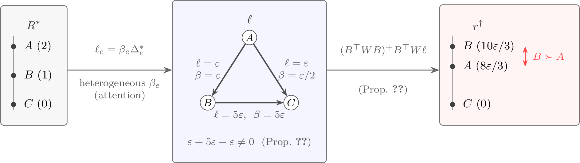
This paper develops the theoretical implications of treating comparisons as attention-limited measurements. The argument proceeds in three steps, each answering a question the previous step raises. Figure 1 previews the central failure the paper isolates, i.e., attention-limited comparisons whose every pairwise majority is correct drive the Bradley–Terry fit to the wrong ranking.
The first step asks when attention-filtered comparisons are compatible with reward fitting at all. Section 2 motivates the channel 2 from a Shannon rational-inattention first-order condition and states it as a reduced-form measurement model. Section 3 then gives an exact answer on a finite comparison graph. A scalar Bradley–Terry reward can represent the observed log odds if and only if their circulation around every cycle vanishes (Proposition 1). Homogeneous attention passes this test, because a common multiplier merely rescales reward; heterogeneous attention generically fails it. So the object that reward fitting presumes need not exist, and the question becomes what a Bradley–Terry learner converges to instead.
The second step characterizes that limit and shows the resulting error is one of kind, not degree. Near the low-information regime, the population Bradley–Terry solution is the weighted projection of the observed log-odds field onto the space of potential fields (Proposition 2), an object shaped by the comparison graph and query distribution as much as by the underlying values. A three-item example makes the danger concrete. The projection ranks item \(B\) above item \(A\) even though \(A\) is deliberatively better and every pairwise majority points in the correct direction (Example 1). One might hope this is an artifact of the Bradley–Terry functional form, to be repaired by a richer model class, a prior, or more data. Proposition 3 shows that this is not the case. Reward, attention, and defaults are not separately identified from passive comparison probabilities, so the same data are consistent with many incompatible reward vectors no matter what estimator consumes them.
The third step explains why these failures are inevitable and what they cost, moving from the Bradley–Terry learner to arbitrary procedures by working at the level of the labels themselves. A comparison label is a one-bit message emitted after costly information acquisition, and its entropy is not its information content. A label can be maximally random while carrying arbitrarily little information about the reward gap (Proposition 4). Per-label mutual and Fisher information about reward scale as \(\beta_z^2\), and when attention is unknown the local information matrix is rank one, so the likelihood sees only the product \(\beta\Delta\) (Proposition 5). This is the local face of the non-identification above. KL and Fano arguments turn the scaling into sample complexity. Distinguishing \(\Delta=\delta\) from \(\Delta=-\delta\) requires on the order of \(1/(\beta^2\delta^2)\) labels, and reward recovery over any hypothesis class is governed by total attended information rather than the number of annotations (Theorem 1).
Finally, Section 5 tests the theory empirically in two settings. In human votes over language-model pairs from Chatbot Arena, the observed log-odds field carries cyclic energy beyond sampling noise, rejecting representation by any scalar score, and the one-eighth law of Proposition 7 prices the misfit to within about ten percent. In a perceptual comparison dataset with response times and gaze, the channel’s ingredients are visible directly. Psychometric slopes vary sixfold across evaluators, gaze appears as an additive default, and response time reveals gap-magnitude information that is absent from single labels alone.
1.0.0.2 Related work.
Reward learning from human feedback and its failure modes. Pairwise comparisons are the standard interface for aligning language models and agentic systems [1]–[5]; direct preference optimization removes the explicit reward model but keeps the Bradley–Terry link between choices and reward differences [6]. A growing literature documents failure modes of this pipeline. Reward models degrade under optimization pressure [17], admit reward hacking through gaps between proxy and target [22], absorb surface regularities such as response length [16], and inherit fundamental limitations of human oversight [23]. We contribute an attention-based account of one such limitation. Even with unlimited data and no optimization pressure, the Bradley–Terry estimand itself can be wrong once evaluator attention is heterogeneous.
Human models in reward inference. Any reward-learning method embeds a model of the human data generator [24]. The classical choices are noiseless or Boltzmann-rational behavior [8]; richer models treat systematic human biases as objects to be learned [25], [26] or cast value learning as a cooperative game between human and machine [27]. The attention-scaled channel is motivated by endogenous attention allocation. Costly evaluation makes the distortion query-specific, correlated with evaluation difficulty, and, as Section 3 shows, unidentifiable from passive labels.
Beyond Bradley–Terry. Motivated in part by intransitivity in human preference data, recent work replaces the scalar-reward assumption with general preference models and solves for von Neumann winners or Nash equilibria of a preference game [28]–[30]. Our results are complementary. The attention-scaled channel shows how cyclic comparison data can arise from heterogeneous attention, and Proposition 7 prices the information that any scalar reward must discard.
Statistical ranking and rational inattention. The statistical ranking literature studies estimation from pairwise comparisons when Bradley–Terry or a parametric relative is correctly specified [10], [11], [31]; we instead characterize the pseudo-true target under the misspecification that attention induces. The potential–cyclic decomposition of Section 4.4 is the combinatorial Hodge decomposition introduced to statistical ranking by [32]; here the cyclic component arises from heterogeneous attention, and we quantify its KL cost for scalar reward fitting. A behavioral motivation is Shannon rational inattention. The generalized-logit structure of optimal behavior follows [19], building on [18], with revealed-preference and discrete-choice formulations in [20] and [21]. We use this theory to motivate, rather than fully identify from first principles, a measurement channel for alignment feedback.
Scalable oversight. The premise that the most alignment-relevant comparisons are the hardest to evaluate motivates scalable-oversight proposals such as recursive reward modeling, debate, and evaluation assistance [12]–[15]. Our lower bounds formalize what such interventions must accomplish. Because sign, ranking, and reward recovery are governed by attended information, an oversight protocol adds value insofar as it raises the attention multiplier on the comparisons that matter, and active query selection [33] cannot substitute for attention it does not change.
2 Model↩︎
2.1 Pairwise reward learning↩︎
Let \(x\in\mathcal{X}\) denote a context, prompt, market state, or initial state, and let \(\mathcal{Y}(x)\) be the feasible candidate set. A comparison query is a triple \[z=(x,y^0,y^1)\in\mathcal{Z},\] and the observed label is \(c\in\{0,1\}\), where \(c=1\) records a choice of \(y^1\) over \(y^0\). Queries are drawn from a distribution \(\rho\) determined by the data-collection policy.
The target is a deliberative reward \(R^*(x,y)\in\mathbb{R}\), interpreted as the evaluation the principal wants the human to apply after processing all reward-relevant information under the intended criterion. Write \[\Delta_z^*=R^*(x,y^1)-R^*(x,y^0)\] for the deliberative difference in query \(z\). A standard reward learner chooses a score function \(r\in\mathcal{R}\) by logistic maximum likelihood, \[\widehat r_n\in\mathop{\mathrm{arg\,max}}_{r\in\mathcal{R}} \frac{1}{n}\sum_{t=1}^n \left\{ c_t\log \sigma(d_r(z_t))+(1-c_t)\log \sigma(-d_r(z_t)) \right\}, \qquad d_r(z)=r(x,y^1)-r(x,y^0), \label{eq:empirical-risk}\tag{3}\] under the maintained hypothesis that \(\mathbb{P}[c=1\mid z]=\sigma(d_r(z))\) for some reward aligned with \(R^*\). The paper studies what comparison data reveal when human labels are instead attention-filtered measurements of deliberative reward.
2.2 Rationally inattentive comparison behavior↩︎
Fix a query \(z\) and let \(\omega\in\Omega_z\) denote the evidence relevant to the comparison: facts in the context, latent consequences of the two candidates, safety implications, or other payoff-relevant information. For the rational-inattention benchmark in this subsection, assume \(\Omega_z\) is finite and the prior \(\mu_z\) has full support. A comparator chooses an attention-decision rule \(\pi_z(a\mid\omega)\) over actions \(a\in\{0,1\}\), where action \(a=1\) means choosing \(y^1\) and action \(a=0\) means choosing \(y^0\). The marginal action probability induced by \(\pi_z\) is \[\bar\pi_z(a)=\sum_{\omega\in\Omega_z}\mu_z(\omega)\pi_z(a\mid\omega).\]
Let \(u_z(a,\omega)\) be the comparator’s payoff, encoding the evaluation criterion the principal intends. The comparator solves the Shannon rational-inattention problem \[\max_{\pi_z} \mathbb{E}_{\omega\sim\mu_z,\,a\sim\pi_z(\cdot\mid\omega)}[u_z(a,\omega)] -\kappa_z \mathrm{I}_z(\omega;a), \label{eq:ri-problem}\tag{4}\] where \(\kappa_z>0\) is the marginal cost of information and \[\mathrm{I}_z(\omega;a) =\sum_{\omega,a}\mu_z(\omega)\pi_z(a\mid\omega) \log\frac{\pi_z(a\mid\omega)}{\bar\pi_z(a)} . \label{eq:mutual-info}\tag{5}\] The next lemma is the standard generalized-logit form of the Shannon solution. It is included to pin down where the attention multiplier and the endogenous marginal action tendency enter.
Lemma 1 (Shannon rational inattention implies generalized logit). At any interior optimum of 4 , \[\pi_z(a\mid\omega) =\frac{\bar\pi_z(a)\exp(u_z(a,\omega)/\kappa_z)}{\sum_{b\in\{0,1\}}\bar\pi_z(b)\exp(u_z(b,\omega)/\kappa_z)} . \label{eq:generalized-logit}\qquad{(1)}\] Consequently, \[\log\frac{\pi_z(1\mid\omega)}{\pi_z(0\mid\omega)} =\alpha_z+\beta_z\{u_z(1,\omega)-u_z(0,\omega)\}, \qquad \alpha_z=\log\frac{\bar\pi_z(1)}{\bar\pi_z(0)},\quad \beta_z=\kappa_z^{-1}. \label{eq:conditional-logodds}\qquad{(2)}\]
Equation ?? is a conditional first-order characterization. The payoff difference is multiplied by the query-specific inverse information cost \(\beta_z\), while the endogenous marginal action tendency \(\alpha_z\) enters additively. It does not by itself pin down the ex-ante marginal label probability obtained by integrating over evidence states, and when the payoff difference is deterministic and nonzero the optimum is a boundary case to which the interior logit formula does not apply. The rest of the paper therefore takes the following equation as a reduced-form marginal measurement channel, motivated by the conditional rational-inattention first-order condition rather than derived from it. The additive term \(\eta_z\) in the reduced form should be read as standing in for the endogenous action tendency \(\alpha_z\) together with genuinely exogenous order, format, and salience effects; Remark 1 gives one environment in which the channel holds exactly.
Definition 1 (Attention-scaled comparison channel). An attention-scaled comparison channel is a map \(z\mapsto q_z\in(0,1)\) satisfying \[q_z=\sigma(\ell_z), \qquad \ell_z=\eta_z+\beta_z\Delta_z^*, \qquad \beta_z\ge 0. \label{eq:attention-channel}\qquad{(3)}\] The case \(\eta_z=0\) and \(\beta_z\equiv\beta>0\) is called homogeneous attention.
Remark 1 (An exact conditional interpretation). There is one environment in which the channel holds exactly rather than as a reduced form. Suppose the evidence state \(\omega\) is realized but unknown to the comparator ex ante, and let \(\Delta_z^*=u_z(1,\omega)-u_z(0,\omega)\) be the payoff difference in the realized state, which is the deliberative difference of Section 2 when the payoff encodes the intended criterion. If the optimum of 4 is interior, Lemma 1 implies that the label distribution conditional on the realized state is exactly \(\sigma(\alpha_z+\beta_z\Delta_z^*)\), which is Definition 1 with \(\eta_z=\alpha_z\). In this paper, the default is endogenous, determined by the prior \(\mu_z\) and the information cost \(\kappa_z\), and this is why priors and salience enter additively rather than being scaled like reward. The reduced form frees \(\eta_z\) from this benchmark to accommodate order and format effects as well.
All graph-theoretic and information-theoretic results below are statements about the reduced-form channel in Definition 1. If \(\beta_z=0\), the comparison label is independent of the deliberative reward difference after conditioning on the default term. Such a query may still produce random-looking labels, but it carries no information about the sign or magnitude of \(\Delta_z^*\) through the reward channel.
With the channel in hand, the paper’s question can be stated. A learner observes the choice probabilities \(q_z\), while the object of interest is \(\Delta_z^*\); what does the former reveal about the latter? Section 3 answers for the standard Bradley–Terry reward learner, at the level of representation and identification. Section 4 then drops the estimator from the picture and answers at the level of information, bounding what any procedure could distinguish with any amount of data.
3 Why Raw Comparisons Are Not Enough↩︎
This section studies the standard Bradley–Terry reward learner under the attention-scaled channel. We first ask whether the observed log odds are compatible with any scalar reward at all, and the answer is a cycle criterion that heterogeneous attention generically violates. Practitioners fit Bradley–Terry whether or not the criterion holds, so the next question is what the fit converges to when it fails. It converges to a projection of the log-odds field, and the projection can reverse the deliberative ranking (Section 3.2). The last question is whether a different parameterization of the reward model could avoid these problems. It cannot, because without further restrictions reward, attention, and defaults are observationally equivalent along a continuum of explanations (Section 3.3).
3.1 Cycle obstructions to scalar representability↩︎
The first question is whether attention-filtered log odds can be represented by any scalar reward at all. This is a purely algebraic question about the structure of the log-odds field, and it has a complete answer. Fix one context and a finite candidate set \(V=\{1,\ldots,m\}\). Let \(G=(V,E)\) be the undirected comparison graph. Choose an arbitrary orientation for each edge \(e=(i,j)\in E\) and let \(q_e=q_{ij}\) be the probability that \(i\) is chosen over \(j\) in that oriented comparison. Define \(\ell_e=\mathop{\mathrm{logit}}(q_e)\), and use the antisymmetric extension \(\ell_{ji}=-\ell_{ij}\) when an edge is traversed against its chosen orientation. Let \(B\in\mathbb{R}^{E\times V}\) be the signed incidence matrix with \((Br)_e=r_i-r_j\) for \(e=(i,j)\). A Bradley–Terry representation of the channel is exactly a potential representation \(\ell=Br\). The only obstruction is circulation around cycles.
Proposition 1 (Cycle consistency). Assume \(G\) is connected and \(q_e\in(0,1)\) on every compared edge. There exists a score vector \(r\in\mathbb{R}^m\) such that \(\ell_e=(Br)_e\) on every edge if and only if \[\sum_{k=1}^K \ell_{i_k i_{k+1}}=0, \qquad i_{K+1}=i_1, \label{eq:cycle-condition}\qquad{(4)}\] for every directed cycle \((i_1,i_2,\ldots,i_K,i_1)\) in \(G\), where reversing an oriented edge changes the sign of its log odds. When such a score exists, it is unique up to an additive constant.
The proposition gives an immediate diagnostic for attention-filtered data. Homogeneous attention is harmless because it merely rescales the potential. Potential defaults are representable but still misaligned, because the fitted reward absorbs the default. Heterogeneous edge-specific attention generally creates nonzero cycle sums.
Corollary 1 (Representability of attention-scaled comparisons). On a finite connected comparison graph, attention-scaled log odds \[\ell_{ij}=\eta_{ij}+\beta_{ij}(R_i^*-R_j^*)\] admit an exact Bradley–Terry reward if and only if their cycle sums vanish. In particular:
if \(\eta_{ij}=0\) and \(\beta_{ij}=\beta>0\) on all edges, then \(r_i=\beta R_i^*\) is an exact representation;
if \(\beta_{ij}=\beta>0\) and \(\eta_{ij}=b_i-b_j\) for some potential \(b\in\mathbb{R}^m\), then \(r_i=\beta R_i^*+b_i\) is an exact representation.
The second case illustrates a subtle failure mode. A default with potential structure, such as a systematic preference for familiar formats or concise answers, is perfectly representable by Bradley–Terry scores. It is nevertheless not deliberative reward; it reverses pairs whenever the default difference dominates the attended reward difference.
3.2 The attention-blind Bradley–Terry target↩︎
A failed cycle criterion does not stop anyone from fitting Bradley–Terry. The population likelihood remains strictly concave, so the fit converges regardless, and the question is what it converges to. The next proposition identifies the limit near the low-information regime as the weighted least-squares projection of the human log-odds field onto the space of potential fields. The fitted reward is therefore not a noisy copy of deliberative value but a graph-dependent compression of it, shaped by the comparison graph and the sampling policy as much as by human values.
Let \(W=\mathop{\mathrm{diag}}(\rho_e)\) collect the edge sampling probabilities, with \(\rho_e>0\) and \(\sum_e\rho_e=1\). Normalize scores by \(\mathbf{1}^\top r=0\). For an oriented edge vector \(\ell\), define the population objective \[L(r;\ell) =\sum_{e\in E}\rho_e \left\{\sigma(\ell_e)\log\sigma((Br)_e) +\bigl(1-\sigma(\ell_e)\bigr)\log\sigma(-(Br)_e)\right\}. \label{eq:population-bt-graph}\tag{6}\]
Proposition 2 (Local projection of log odds). Suppose \(G\) is connected, \(\rho_e>0\) on every edge, and \(\|\ell\|_\infty\le \varepsilon\). Let \(r^\dagger(\ell)\) be the unique maximizer of 6 on the subspace \(\mathbf{1}^\top r=0\). Then, as \(\varepsilon\to0\), \[r^\dagger(\ell) = (B^\top W B)^+B^\top W\ell + O(\varepsilon^3), \label{eq:projection-formula}\qquad{(5)}\] where \((\cdot)^+\) denotes the Moore–Penrose inverse acting on the subspace orthogonal to constants. The remainder is in Euclidean norm and is uniform over sufficiently small \(\|\ell\|_\infty\).
The projection in Equation ?? discards all cyclic components of the human log odds. The following example shows that the induced error is not merely cardinal; it can reverse the learned ranking.
Example 1 (A three-item projection reversal). Consider one context with candidates \(A,B,C\) and deliberative rewards \[R_A^*=2, \qquad R_B^*=1, \qquad R_C^*=0.\] There is no default bias. Human log odds for the higher-reward item over the lower-reward item are \[\ell_{AB}=\varepsilon, \qquad \ell_{AC}=\varepsilon, \qquad \ell_{BC}=5\varepsilon, \label{eq:example-logodds}\qquad{(6)}\] for small \(\varepsilon>0\). These log odds arise from the scalar attention channel with \(\beta_{AB}=\varepsilon\), \(\beta_{AC}=\varepsilon/2\), and \(\beta_{BC}=5\varepsilon\). Thus every individual pairwise majority points in the deliberatively correct direction. Sampling the three pairs equally and normalizing \(r_C=0\), Proposition 2, equivalently the direct first-order calculation in the appendix, yields \[r_A^\dagger=\frac{8}{3}\varepsilon+O(\varepsilon^3), \qquad r_B^\dagger=\frac{10}{3}\varepsilon+O(\varepsilon^3), \qquad r_C^\dagger=0. \label{eq:example-scores}\qquad{(7)}\] For sufficiently small \(\varepsilon\), the attention-blind Bradley–Terry target ranks \(B\) above \(A\) although \(A\) is deliberatively best. The reversal is not a knife-edge feature of the expansion; solving the population first-order conditions exactly preserves the same ordering at moderate scales such as \(\varepsilon=0.4\).
3.3 Non-identification↩︎
Example 1 might suggest that the problem lies with the Bradley–Terry functional form, and that a richer model class, a Bayesian prior over rewards, or simply more data would recover the deliberative ranking. The deeper obstacle is that comparison probabilities alone cannot disentangle reward, attention, and defaults, so any method that consumes only passive labels inherits the same ambiguity. The next proposition makes this point in finite-dimensional form.
Proposition 3 (Non-identification of reward, attention, and defaults). Fix comparison probabilities \(q_{ij}\in(0,1)\) on a finite set of oriented pairs, and write \(\ell_{ij}=\mathop{\mathrm{logit}}(q_{ij})\).
For any candidate reward vector \(v\in\mathbb{R}^m\) and any nonnegative attention multipliers \(\beta_{ij}\ge0\), the defaults \[\eta_{ij}=\ell_{ij}-\beta_{ij}(v_i-v_j) \label{eq:eta-rationalization}\qquad{(8)}\] rationalize the data through the attention-scaled channel.
Suppose defaults are restricted to zero. If, for every compared pair, either \(v_i\ne v_j\) and \(\ell_{ij}\,(v_i-v_j)\ge0\), or \(v_i=v_j\) and \(\ell_{ij}=0\), then the same data are rationalized by the pair-specific multipliers \[\beta_{ij}=\frac{\ell_{ij}}{v_i-v_j} \label{eq:beta-rationalization}\qquad{(9)}\] on all compared pairs with \(v_i\ne v_j\), and by any nonnegative \(\beta_{ij}\) on zero-gap pairs with \(\ell_{ij}=0\).
This proposition is the formal reason that a Bayesian prior, a larger neural reward model, or more passive samples cannot by itself recover deliberative reward. Without restrictions that distinguish reward from attention and defaults, the likelihood is flat along observationally equivalent explanations.
Non-identification says the likelihood is flat; it does not yet say why the flatness arises, or how much data it costs even where the parameters are partially informative. Both questions have exact answers once the label is treated as a communication channel and its information content is accounted for directly. That accounting is the subject of the next section.
4 Information-Theoretic Limits of Reward Learning↩︎
Section 3 located three failures of the Bradley–Terry reward learner. The log odds need not be representable by any scalar reward, the fit converges to a graph-dependent projection, and the likelihood is flat across observationally equivalent explanations. All three statements concern one particular estimator, so one might still hope that a cleverer use of the same labels escapes them. This section shows that they are instead properties of the labels themselves, by re-deriving each failure at the level of information, where no estimator appears. The weak-signal ambiguity becomes a separation between label entropy and reward information (Section 4.1); non-identification becomes a rank-one information matrix (Section 4.2); the estimation failures become sample-complexity lower bounds that bind every procedure, adaptive or not (Section 4.3); and the cycle obstruction acquires an exact price in KL divergence (Section 4.4). Throughout, a comparison label is viewed as a binary message emitted after information acquisition. Its entropy may be high while the information it carries about deliberative reward is arbitrarily small. Defaults are suppressed when they are not essential, since adding a known default shifts the log odds but does not change the information bottleneck created by \(\beta\).
4.1 High label entropy is not high reward information↩︎
A nearly even split of labels is often treated as the most informative region of a logistic model because the Bernoulli variance is largest near one half. That intuition is incomplete. If the split is even because attention is near zero, the label may be maximally random while revealing almost nothing about reward.
Consider a single pair and let \(\Delta\) be an unknown deliberative reward difference with a finite prior distribution \(\Pi\). Conditional on \(\Delta\), the observed label satisfies \[C\mid \Delta \sim \mathop{\mathrm{Bernoulli}}\bigl(\sigma(\eta+\beta\Delta)\bigr), \qquad \beta\ge0. \label{eq:random-gap-channel}\tag{7}\] Let \(\mathsf{H}(C)\) denote the entropy of the marginal label and \(\mathrm{I}(\Delta;C)\) the mutual information between the reward gap and the label, measured in nats.
Proposition 4 (Entropy-information separation). In the channel 7 :
if \(\beta=0\), then \(C\) is independent of \(\Delta\), so \(\mathrm{I}(\Delta;C)=0\);
if, in addition, \(\eta=0\), then \(C\) is a fair coin, so \(\mathsf{H}(C)=\log 2\) while \(\mathrm{I}(\Delta;C)=0\);
if the prior on \(\Delta\) has finite support, then as \(\beta\to0\), \[\mathrm{I}(\Delta;C) =\frac{1}{2}\sigma(\eta)\bigl(1-\sigma(\eta)\bigr)\beta^2\mathop{\mathrm{Var}}(\Delta)+O(\beta^3). \label{eq:mi-small-beta}\qquad{(10)}\]
Thus a \(50\)–\(50\) outcome has two distinct interpretations. It may mean the reward gap is close to zero, or it may mean the channel is low-transmission because \(\beta\) is small. The entropy of the label alone cannot distinguish these cases.
4.2 Fisher information and local non-identification↩︎
Proposition 4 is a statement about a prior over the gap. The same distinction appears in local, estimation-theoretic form through Fisher information, and in that form it also exposes the mechanism behind the non-identification of Proposition 3. In the standard Bradley–Terry model, one label contains the most local information about the reward difference near a \(50\)–\(50\) split. Under the attention-scaled channel, that maximum is multiplied by \(\beta^2\).
Proposition 5 (Fisher information collapse and rank-one information). For one comparison with \[C\sim \mathop{\mathrm{Bernoulli}}(q), \qquad q=\sigma(\eta+\beta\Delta), \label{eq:single-pair-fisher}\qquad{(11)}\] the following hold.
If \(\eta\) and \(\beta\) are known, the Fisher information in one label about \(\Delta\) is \[\mathcal{I}_\Delta(\Delta)=\beta^2 q(1-q)\le \frac{\beta^2}{4}. \label{eq:fisher-known-beta}\qquad{(12)}\]
If \(\eta\) is known but \((\Delta,\beta)\) are both unknown, the Fisher information matrix for \((\Delta,\beta)\) is \[\mathcal{I}_{(\Delta,\beta)} =q(1-q) \begin{pmatrix} \beta^2 & \beta\Delta \\ \beta\Delta & \Delta^2 \end{pmatrix} =q(1-q) \begin{pmatrix}\beta\\ \Delta\end{pmatrix} \begin{pmatrix}\beta & \Delta\end{pmatrix}, \label{eq:fisher-rank-one}\qquad{(13)}\] and therefore has rank at most one.
If \(\eta\), \(\Delta\), and \(\beta\) are all unknown, the Fisher information matrix for \((\eta,\Delta,\beta)\) is \[\mathcal{I}_{(\eta,\Delta,\beta)} =q(1-q) \begin{pmatrix}1\\ \beta\\ \Delta\end{pmatrix} \begin{pmatrix}1 & \beta & \Delta\end{pmatrix}, \label{eq:fisher-rank-one-eta}\qquad{(14)}\] and again has rank at most one.
When \(\beta\) is constrained to be nonnegative, the usual regular Fisher-information interpretation for parameters involving \(\beta\) applies at interior points \(\beta>0\); at the boundary \(\beta=0\), the displays are local derivative formulas for the logit index.
The first claim gives a sample-complexity penalty, since low attention reduces per-label information about reward quadratically. The rank-one claims give a local version of Proposition 3. The likelihood identifies the log-odds index \(\eta+\beta\Delta\), not the reward gap, the attention multiplier, and the default separately.
4.3 Lower bounds for sign and ranking recovery↩︎
Fisher information measures local difficulty; the operational question is global. How many labels does it take to answer the coarsest question the data could settle, namely which of the two candidates is better? The next result shows that ordinal recovery, too, is bought only with attended information. To isolate the effect, consider the clean channel with no default and known attention, \[C\sim \mathop{\mathrm{Bernoulli}}(\sigma(\beta\Delta)). \label{eq:clean-sign-channel}\tag{8}\] The task is to decide whether \(\Delta=\delta\) or \(\Delta=-\delta\) for a fixed \(\delta>0\).
Proposition 6 (KL lower bound for sign recovery). Let \(P_+\) be the distribution of one label under \(\Delta=\delta\) and \(P_-\) the distribution under \(\Delta=-\delta\) in 8 . If \(\beta=0\), then \(P_+=P_-\) and no test can have worst-case error probability below \(1/2\). If \(\beta>0\), then \[D_{\mathrm{KL}}(P_+\|P_-) =\beta\delta\tanh\left(\frac{\beta\delta}{2}\right) \le \frac{(\beta\delta)^2}{2}. \label{eq:sign-kl}\qquad{(15)}\] For any test based on \(n\) independent labels and \(\beta>0\), if the worst-case probability of sign error is at most \(\alpha<1/2\), then necessarily \[n\ge \frac{2(1-2\alpha)^2}{\beta\delta\tanh(\beta\delta/2)} \ge \frac{4(1-2\alpha)^2}{\beta^2\delta^2}. \label{eq:sign-lower-bound}\qquad{(16)}\] Consequently, without a positive lower bound on attention, no uniform finite-sample sign guarantee is possible.
The lower bound depends on the product \(\beta\delta\). Bradley–Terry interprets a small product as a small reward gap. The attention-scaled model shows that it may instead be a large reward gap passing through a low-attention channel.
The same logic extends from one pair to many reward hypotheses. Let \(\Theta\) be a finite set of possible reward functions and suppose the learner observes labels \(C_1,\ldots,C_n\), possibly under adaptively chosen queries. Let \(H_{t-1}\) denote the history before label \(t\), including previous labels, adaptively chosen queries, and any external randomization used by the query rule. Let \(P_{\theta,t}(\cdot\mid h_{t-1})\) denote the conditional distribution of label \(t\) under reward hypothesis \(\theta\) and history \(h_{t-1}\).
Theorem 1 (Fano bound for attention-limited reward recovery). Assume \(\theta\) is uniform on a finite class \(\Theta\) with \(|\Theta|=M\ge2\). Suppose that for every time \(t\), every history \(h_{t-1}\) with positive probability under the joint mixture distribution induced by the uniform prior over \(\Theta\), and every pair \(\theta,\theta'\in\Theta\), \[D_{\mathrm{KL}}\bigl(P_{\theta,t}(\cdot\mid h_{t-1})\,\|\,P_{\theta',t}(\cdot\mid h_{t-1})\bigr) \le d_t. \label{eq:per-label-kl-bound}\qquad{(17)}\] Then any estimator based on the observed history satisfies \[\mathbb{P}[\widehat\theta\ne\theta] \ge 1-\frac{\sum_{t=1}^n d_t+\log 2}{\log M}. \label{eq:fano-bound}\qquad{(18)}\]
In attention-scaled logistic channels, the constants \(d_t\) are of order \(\beta_t^2\) for small attended reward separations. The bound therefore says that reward recovery is limited by total attended information \(\sum_t d_t\), not simply by the number of labels. Repeating low-attention comparisons can be much less valuable than collecting fewer high-attention comparisons.
4.4 Potential information and cyclic information on comparison graphs↩︎
The bounds so far concern single pairs and finite hypothesis classes. Returning to the comparison graph closes the loop with Section 3. The cycle obstruction, similarly, has an information-theoretic meaning, and the projection of Proposition 2 turns out to be the object that discards it. A scalar reward can represent only potential fields on the comparison graph. The part of the observed log-odds field orthogonal to all potentials is cyclic comparison information, present in the human comparisons but impossible to encode in any scalar reward. The decomposition below is the combinatorial Hodge decomposition of [32], applied to the weighted log-odds field generated by the attention-scaled channel.
Let the weighted inner product on edge fields be \[\langle a,b\rangle_W=a^\top Wb, \qquad \|a\|_W^2=a^\top Wa.\] Let \(\mathcal{P}=\operatorname{im}(B)\) be the potential subspace. Define \[r^H=(B^\top W B)^+B^\top W\ell, \qquad \ell^{\mathrm{pot}}=Br^H, \qquad \ell^{\mathrm{cyc}}=\ell-\ell^{\mathrm{pot}}. \label{eq:hodge-decomposition}\tag{9}\]
Proposition 7 (Cyclic information loss of scalar rewards). Suppose \(G\) is connected, \(W=\mathop{\mathrm{diag}}(\rho_e)\) has positive diagonal entries, and \(\|\ell\|_\infty\le\varepsilon\). Then:
\(\ell=\ell^{\mathrm{pot}}+\ell^{\mathrm{cyc}}\) is the weighted orthogonal decomposition of the log-odds field into the potential subspace and its orthogonal complement: \(B^\top W\ell^{\mathrm{cyc}}=0\) and \[\|\ell\|_W^2=\|\ell^{\mathrm{pot}}\|_W^2+\|\ell^{\mathrm{cyc}}\|_W^2. \label{eq:hodge-pythagorean}\qquad{(19)}\]
The best scalar-reward approximation in weighted KL divergence satisfies \[\begin{align} &\inf_{r:\,\mathbf{1}^\top r=0} \sum_{e\in E}\rho_e\, D_{\mathrm{KL}}\Bigl( \mathop{\mathrm{Bernoulli}}(\sigma(\ell_e))\,\Big\|\, \mathop{\mathrm{Bernoulli}}(\sigma((Br)_e)) \Bigr) \notag\\ &= \frac{1}{8}\|\ell^{\mathrm{cyc}}\|_W^2+O(\varepsilon^3), \label{eq:cyclic-kl-loss} \end{align}\qquad{(20)}\] where the remainder is uniform over sufficiently small \(\|\ell\|_\infty\).
The coefficient \(r^H\) in 9 is computed by the same operator as the pseudo-true target in ?? . To first order, the attention-blind Bradley–Terry limit is the potential component of the human log odds. Proposition 7 therefore prices what Proposition 2 discards. The cycle obstruction is not merely a consistency condition. It quantifies how much comparison information is irreducibly non-reward-like, and the cyclic energy measures the second-order information loss of compressing the human comparison channel to its potential component.
5 Empirical Case Studies↩︎
The theory leaves two observable footprints. The geometric footprint is cyclic energy in comparison fields, and the mechanistic footprint is that measurements of the evaluation process, such as response times and gaze, should carry information that labels do not. Two case studies check one footprint each.
5.1 Cyclic comparison information in Arena votes↩︎
The theory predicts that the log-odds field of real comparison data need not be a potential field, and Proposition 7 prices what any scalar score then discards. We test this signature on a canonical human preference dataset, \(57{,}477\) pairwise battles between \(64\) language models collected on Chatbot Arena [34].2 Items are models, edges are model pairs, and labels are human votes, so the empirical vote frequencies provide exactly the weight matrix \(W\) of Section 3. We drop ties (\(31\%\) of battles), keep pairs with at least \(100\) decisive votes, and restrict to the largest connected component, which leaves \(m=32\) models, \(74\) pairs, \(15{,}001\) votes, and a cycle space of dimension \(74-31=43\). Edge log odds use the Haldane–Anscombe estimate \(\hat{q}_e=(w_e+\tfrac12)/(n_e+1)\).
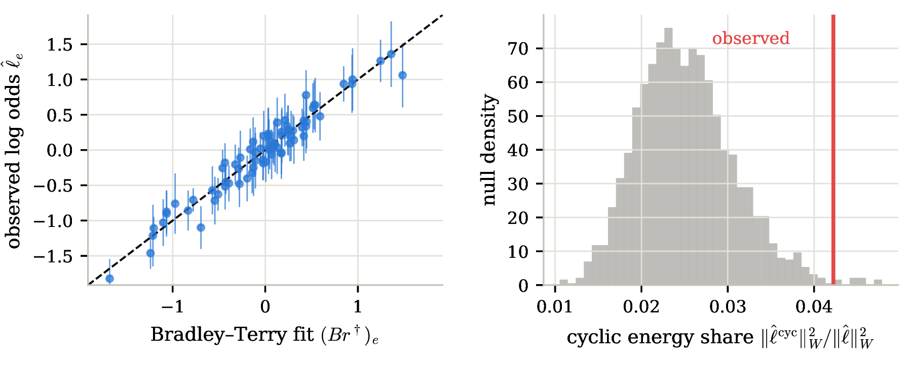
Sampling noise alone creates cyclic energy, so significance is judged against a parametric bootstrap null. We fit Bradley–Terry by weighted maximum likelihood, regenerate binomial votes at the observed \(n_e\) two thousand times, and recompute the cyclic energy share of each regenerated field. The observed share is \(4.2\%\), against a null mean of \(2.5\%\) and a null \(95\)th percentile of \(3.5\%\), for a bootstrap \(p\)-value of \(0.008\) (Figure 2); the likelihood-ratio statistic gives the same verdict (\(70.6\) on \(43\) degrees of freedom, bootstrap \(p=0.007\)). The hypothesis that some scalar score generates these win rates is rejected at the one percent level.
The misfit is small but priced accurately. The best scalar fit loses \(0.0034\) bits per comparison in weighted KL, and the prediction \(\tfrac18\|\hat{\ell}^{\mathrm{cyc}}\|_W^2\) of Proposition 7 is \(0.0038\) bits, a ratio of \(0.89\), even though the largest observed log odds is near \(1.8\) and the proposition’s small-\(\varepsilon\) hypothesis is far from satisfied. Part of the raw loss reflects sampling noise; the deviance in excess of its degrees of freedom gives a rough noise-corrected estimate of the population-level misfit near \(0.0013\) bits per comparison. Individual triangle circulations reach at most \(z\approx3.0\), which is unremarkable given the number of triangles examined, so the evidence lies in the global excess rather than in any single cycle; we note, without attaching significance, that the top-ranked triangles involve closely related model versions such as claude-2.1, gpt-4-0314, and gpt-4-1106-preview.
The excess cyclic energy survives vote thresholds of \(50\) and \(200\) per pair (bootstrap \(p=0.046\) and \(0.008\)). Counting ties as half wins shrinks every log odds toward zero and weakens the excess, to \(p=0.06\) on the same graph and to insignificance when the threshold also admits sparsely compared pairs, consistent with dilution by a large mass of uninformative labels. Two caveats bound the interpretation. The votes aggregate over prompts and annotators, so cyclic energy can also arise from aggregation rather than per-query attention, and the analysis conditions on the pairs the platform chose to sample. What the case study establishes is a statistical rejection of every scalar score for this comparison data, at a misfit priced well by the one-eighth law; the finding is consistent with, though not unique evidence for, the attention mechanism. A self-contained script reproduces all numbers.
5.2 Response times carry information that labels do not↩︎
The second footprint concerns the channel itself, and it needs data in which the deliberative gap and the evaluator’s information acquisition are both measured. The perceptual comparison dataset of [35] provides both.3 Twenty-five participants made \(31{,}854\) binary comparisons between two rotated bars, choosing the one closer to a target orientation, with angular distances set by the experimenter; the quality gap \(\Delta\in\{-3,\ldots,3\}\) is therefore ground truth rather than a rating proxy, and every trial records the choice, the response time, and gaze fixations. Pooled choices follow a logistic in \(\Delta\) with slope \(1.14\), and per-participant slopes range from \(0.45\) to \(2.70\), a factor of six (Figure 3, left). The same objective gap passes through channels of very different gain across evaluators. The reduced form absorbs attention, effort, and acuity alike into \(\beta\), so this is heterogeneous \(\beta\) measured directly, whatever its source; and because preference datasets pool annotators over different pairs, evaluator-level heterogeneity of this size induces the edge-level heterogeneity that generates cyclic energy of the kind found in Section 5.1.
The headline is an information decomposition. Because the design is symmetric, a single label reveals which item is better but almost nothing about by how much; empirically the label carries \(0.33\) bits about the sign of the gap and \(0.0001\) bits about its magnitude. Response time carries \(0.035\) bits per trial about the magnitude (permutation-corrected, \(p<0.002\)), while the label carries essentially none; mean response time falls from \(2.2\) seconds on ties to \(1.4\) seconds at the largest gap (Figure 3, right). Repeated labels do not close this gap, since they reveal only the confounded index \(\beta\Delta\) of Proposition 5, while response time gives a reading from outside the label channel. The quantity an annotation protocol needs in order to separate a near-tie from a large-but-unresolved gap is absent from the label and present in the response time, which is exactly the measurement the theory recommends collecting.
Gaze is associated with an additive shift of the kind the default \(\eta\) describes. At fixed \(\Delta\), one second of relative dwell toward an item is associated with a \(0.91\) increase in its choice log odds (standard error \(0.03\)), about as much as a full quality level, consistent with the gaze bias documented by [36]; the association is observational, and gaze may follow an emerging choice as well as shape it. Two further caveats apply. The task is perceptual rather than preferential, and response time is endogenous to difficulty, so these are the channel’s ingredients observed in a controlled comparison task rather than in RLHF annotation itself. Annotation platforms typically record decision latency and could release it; the analysis here is what that would enable.
![Figure 3: Choices and response times in a perceptual comparison task [35]; 25 participants, 31{,}854 trials. Left: psychometric curves per participant (gray) and pooled (blue); slopes vary by a factor of six across evaluators. Right: mean response time against gap magnitude, per participant and pooled with 95\% intervals. The label carries 0.33 bits about the sign of the gap and 0.0001 bits about its magnitude, while response time carries 0.035 bits about the magnitude.](/article/2607.04590/figures/fig_attention.png "fig:")
6 Conclusion↩︎
Reward learning from pairwise comparisons changes qualitatively when humans are rationally inattentive. The reduced-form attention-scaled channel motivated by Shannon rational inattention does not simply add noise to reward differences; it scales them by query-dependent attention and adds defaults that do not scale with reward. Raw comparison log odds therefore need not form a potential field, the Bradley–Terry pseudo-true reward can reverse the deliberative ranking, and reward is not separately identified from attention or defaults. The information-theoretic analysis explains why these are not mere modeling inconveniences. A near \(50\)–\(50\) label may reflect true closeness or an attention bottleneck, per-label information about reward scales as \(\beta^2\), unknown attention makes the local information matrix rank one, and KL and Fano bounds show that sign, ranking, and reward recovery require total attended information rather than more labels. On graphs, the Hodge decomposition prices the cyclic comparison information that no scalar reward can represent. The case studies find that signature in Chatbot Arena votes, with the one-eighth law pricing the misfit accurately, and show in a perceptual comparison task that response times and gaze carry information about the evaluation process that labels do not.
The main implication for alignment practice is that reward learning under bounded attention is measurement under an endogenous information constraint, not curve fitting. Annotation protocols should treat weak pairwise signals as ambiguous between true indifference and failed evaluation, and should be especially suspicious of near-even splits on safety-relevant pairs, where the hard-because-hidden interpretation is most plausible. Our bounds also give scalable-oversight interventions [13]–[15] a precise target. Such interventions help insofar as they raise the attention multiplier on the comparisons that matter, since no amount of passive relabeling can substitute for attended information. Natural next steps include oversight interventions that demonstrably shift attention, response-time or deliberation-effort measurement as proxies for information acquisition, partial-identification bounds under explicit attention constraints, and extensions of the graph information decomposition to function approximation over contexts and trajectories.
7 Proofs↩︎
7.1 Proof of Lemma 1↩︎
Proof. Fix \(z\) and suppress the query subscript. Write \(u(a,\omega)=u_z(a,\omega)\), \(\mu=\mu_z\), \(\kappa=\kappa_z\), and \(\pi=\pi_z\). Because the optimum is interior, \(\pi(a\mid\omega)>0\) and \(\bar\pi(a)>0\) for both actions. The mutual information can be written as \[\mathrm{I}(\omega;a) =\sum_{\omega,a}\mu(\omega)\pi(a\mid\omega)\log\pi(a\mid\omega) -\sum_a \bar\pi(a)\log\bar\pi(a).\] For each \(a\) and \(\omega\), \[\frac{\partial \mathrm{I}}{\partial \pi(a\mid\omega)} =\mu(\omega)\{\log\pi(a\mid\omega)+1\} -\mu(\omega)\{\log\bar\pi(a)+1\} =\mu(\omega)\log\frac{\pi(a\mid\omega)}{\bar\pi(a)}.\] The Lagrangian for the simplex constraints \(\sum_a\pi(a\mid\omega)=1\) is \[\mathcal{L}(\pi,\lambda) =\sum_{\omega,a}\mu(\omega)\pi(a\mid\omega)u(a,\omega) -\kappa\mathrm{I}(\omega;a) +\sum_\omega\lambda_\omega\left(\sum_a\pi(a\mid\omega)-1\right).\] The first-order condition for an interior optimum is \[\mu(\omega)u(a,\omega) -\kappa\mu(\omega)\log\frac{\pi(a\mid\omega)}{\bar\pi(a)} +\lambda_\omega=0.\] Since \(\mu(\omega)>0\), this is equivalent to \[\pi(a\mid\omega)=\bar\pi(a)\exp\{u(a,\omega)/\kappa+m(\omega)\},\] where \(m(\omega)=\lambda_\omega/(\kappa\mu(\omega))\) is independent of \(a\). Enforcing \(\sum_a\pi(a\mid\omega)=1\) determines the normalizing factor and gives Equation ?? . Taking the ratio between actions \(1\) and \(0\) gives Equation ?? with \(\alpha_z=\log\{\bar\pi_z(1)/\bar\pi_z(0)\}\) and \(\beta_z=1/\kappa_z\). ◻
7.2 Proof of Proposition 1↩︎
Proof. If \(\ell=Br\), then the sum of \(\ell\) around any directed cycle telescopes: \[\sum_{k=1}^K \ell_{i_k i_{k+1}} =\sum_{k=1}^K(r_{i_k}-r_{i_{k+1}})=0.\] Conversely, assume all directed cycle sums are zero. Fix a reference vertex \(v_0\). For any vertex \(i\), choose a path \(P_i\) from \(i\) to \(v_0\) and define \(r_i\) as the signed sum of \(\ell\) along that path, with an edge contributing \(\ell_{ab}\) when traversed in its chosen orientation \((a,b)\) and \(-\ell_{ab}\) when traversed in reverse. If two paths from \(i\) to \(v_0\) produced different sums, traversing one path and then the reverse of the other would give a closed walk with nonzero total circulation. Removing repeated vertices decomposes that closed walk into simple cycles, at least one of which would have nonzero circulation, contradicting the assumption. Hence \(r_i\) is well-defined.
For an oriented edge \(e=(i,j)\), compare the path from \(i\) to \(v_0\) with the path that first traverses \(e\) from \(i\) to \(j\) and then follows the chosen path from \(j\) to \(v_0\). Path independence gives \(r_i=\ell_{ij}+r_j\), so \(r_i-r_j=\ell_{ij}\). Thus \(\ell=Br\). If \(r\) and \(r'\) both represent \(\ell\), then \(r_i-r_j=r'_i-r'_j\) on every edge, so \(r-r'\) is constant on every connected component. Since \(G\) is connected, the difference is a global additive constant. ◻
7.3 Proof of Corollary 1↩︎
Proof. The first sentence follows by substituting \(\ell_{ij}=\eta_{ij}+\beta_{ij}(R_i^*-R_j^*)\) into Proposition 1. If \(\eta_{ij}=0\) and \(\beta_{ij}=\beta\), then \(\ell_{ij}=\beta R_i^*-\beta R_j^*\), so \(r_i=\beta R_i^*\) represents the field. If \(\eta_{ij}=b_i-b_j\) and \(\beta_{ij}=\beta\), then \[\ell_{ij}=(\beta R_i^*+b_i)-(\beta R_j^*+b_j),\] so \(r_i=\beta R_i^*+b_i\) represents the field. ◻
7.4 Proof of Proposition 2↩︎
Proof. The objective in 6 is continuous and concave in \(r\). It is coercive on the normalized subspace \(\mathbf{1}^\top r=0\): if \(\|r\|\to\infty\) with \(\mathbf{1}^\top r=0\), then, because \(B\) is injective on \(\mathbf{1}^\perp\) in finite dimensions, \(\|Br\|_\infty\to\infty\). Since \(\sigma(\ell_e)\in(0,1)\) for every finite \(\ell_e\), the Bernoulli logistic term on any edge whose fitted logit diverges tends to \(-\infty\), while the remaining edge terms are nonpositive. Hence \(L(r;\ell)\to-\infty\) along diverging normalized sequences, so a maximizer exists. On \(\mathbf{1}^\perp\), the objective is strictly concave because \(G\) is connected and all \(\rho_e\) are positive: if \(Br\ne Br'\) on some edge, strict concavity of the Bernoulli log-likelihood is strict along that edge, and if \(Br=Br'\) then \(r-r'\) is constant and therefore zero on the normalized subspace. Hence the maximizer is unique.
The first-order condition is \[B^\top W\{\sigma(\ell)-\sigma(Br)\}=0. \label{eq:graph-foc-proof}\tag{10}\] At \(\ell=0\), the unique normalized solution is \(r=0\). The derivative of the left-hand side of 10 with respect to \(r\) at \((\ell,r)=(0,0)\) is \(-(1/4)B^\top W B\), which is nonsingular on \(\mathbf{1}^\perp\) because \(G\) is connected and \(W\) has positive diagonal entries. The implicit-function theorem therefore gives a smooth map \(r^\dagger(\ell)\) in a neighborhood of zero, with \(r^\dagger(0)=0\) and \(\|r^\dagger(\ell)\|=O(\|\ell\|)\).
For \(|t|\) small, \(\sigma(t)=1/2+t/4+O(t^3)\); the quadratic term is absent because \(\sigma(t)-1/2\) is odd. Since \(\|\ell\|_\infty\le\varepsilon\) and \(\|Br^\dagger(\ell)\|_\infty=O(\varepsilon)\), substituting this expansion into 10 yields \[B^\top W\left\{\frac{\ell-Br^\dagger(\ell)}{4}\right\}=O(\varepsilon^3).\] Multiplying by \(4\) and solving on \(\mathbf{1}^\perp\) gives \[r^\dagger(\ell)=(B^\top W B)^+B^\top W\ell+O(\varepsilon^3),\] with a uniform remainder on a sufficiently small neighborhood of zero for the fixed finite graph and fixed positive weights. ◻
7.5 Derivation for Example 1↩︎
Proof. Let \(r_A=x\), \(r_B=y\), and \(r_C=0\). With equal edge weights, the Bradley–Terry fitted probabilities are \[p_{AB}=\sigma(x-y),\qquad p_{AC}=\sigma(x),\qquad p_{BC}=\sigma(y).\] The true probabilities corresponding to ?? are \[q_{AB}=\sigma(\varepsilon),\qquad q_{AC}=\sigma(\varepsilon),\qquad q_{BC}=\sigma(5\varepsilon).\] The first-order conditions for \(x\) and \(y\) are \[\begin{align} (q_{AB}-p_{AB})+(q_{AC}-p_{AC})&=0,\\ -(q_{AB}-p_{AB})+(q_{BC}-p_{BC})&=0. \end{align}\] Using \(\sigma(t)=1/2+t/4+O(t^3)\) and the smoothness of the optimum from Proposition 2, the first-order terms satisfy \[2x-y=2\varepsilon, \qquad 2y-x=4\varepsilon.\] Solving gives \(x=8\varepsilon/3\) and \(y=10\varepsilon/3\). The omitted terms are \(O(\varepsilon^3)\) by the same Taylor expansion and implicit-function argument used in Proposition 2. ◻
7.6 Proof of Proposition 3↩︎
Proof. For arbitrary \(v\) and nonnegative multipliers \(\beta_{ij}\), define \(\eta_{ij}\) by ?? . Then \[\sigma\{\eta_{ij}+\beta_{ij}(v_i-v_j)\} =\sigma(\ell_{ij})=q_{ij},\] which proves the first claim. For the second claim, first consider a compared pair with \(v_i\ne v_j\). The condition \(\ell_{ij}\,(v_i-v_j)\ge0\) makes ?? nonnegative, and it satisfies \[\sigma\{\beta_{ij}(v_i-v_j)\}=\sigma(\ell_{ij})=q_{ij}.\] If \(v_i=v_j\), the stated condition gives \(\ell_{ij}=0\), so setting, for example, \(\beta_{ij}=0\) yields \(\sigma\{\beta_{ij}(v_i-v_j)\}=\sigma(0)=q_{ij}\). Thus all compared pairs are rationalized with zero defaults. ◻
7.7 Proof of Proposition 4↩︎
Proof. If \(\beta=0\), then \(\mathbb{P}[C=1\mid\Delta]=\sigma(\eta)\) for every value of \(\Delta\), so the conditional distribution of \(C\) is independent of \(\Delta\) and \(\mathrm{I}(\Delta;C)=0\). If also \(\eta=0\), then \(\sigma(\eta)=1/2\), so \(C\) is a fair coin and \(\mathsf{H}(C)=\log2\).
For the expansion, let \(q_0=\sigma(\eta)\) and \(s=q_0(1-q_0)\). Because the prior has finite support, all Taylor remainders below are uniform over the support of \(\Delta\). Write \(q_\beta(\Delta)=\sigma(\eta+\beta\Delta)\). Then \[q_\beta(\Delta)=q_0+s\beta\Delta+O(\beta^2), \qquad \bar q_\beta:=\mathbb{E}[q_\beta(\Delta)]=q_0+s\beta\mathbb{E}[\Delta]+O(\beta^2).\] The mutual information is \[\mathrm{I}(\Delta;C) =\mathbb{E}\left[D_{\mathrm{KL}}\bigl(\mathop{\mathrm{Bernoulli}}(q_\beta(\Delta))\,\|\,\mathop{\mathrm{Bernoulli}}(\bar q_\beta)\bigr)\right].\] For Bernoulli parameters \(u\) and \(v\) in a compact subinterval of \((0,1)\), \[D_{\mathrm{KL}}(\mathop{\mathrm{Bernoulli}}(u)\|\mathop{\mathrm{Bernoulli}}(v)) =\frac{(u-v)^2}{2q_0(1-q_0)}+O(|u-v|^3+|v-q_0||u-v|^2).\] Here \[q_\beta(\Delta)-\bar q_\beta=s\beta(\Delta-\mathbb{E}\Delta)+O(\beta^2),\] so \[\mathrm{I}(\Delta;C) =\frac{1}{2s}\mathbb{E}\left[s^2\beta^2(\Delta-\mathbb{E}\Delta)^2\right]+O(\beta^3) =\frac{1}{2} s\beta^2\mathop{\mathrm{Var}}(\Delta)+O(\beta^3),\] which is ?? . ◻
7.8 Proof of Proposition 5↩︎
Proof. For a Bernoulli observation with parameter \(q=\sigma(s)\) and scalar index \(s\), the score with respect to \(s\) is \(C-q\) and the Fisher information for \(s\) is \(q(1-q)\). By the chain rule, for any parameter vector \(\theta\) entering only through \(s(\theta)\), \[\mathcal{I}_\theta=q(1-q)\,\nabla s(\theta)\nabla s(\theta)^\top.\] If \(s=\eta+\beta\Delta\) and \(\eta,\beta\) are known, then \(\partial s/\partial\Delta=\beta\), giving ?? . Since \(q(1-q)\le1/4\), the upper bound follows. If \(\eta\) is known and \(\theta=(\Delta,\beta)\), then \(\nabla s=(\beta,\Delta)^\top\), giving ?? . If \(\theta=(\eta,\Delta,\beta)\), then \(\nabla s=(1,\beta,\Delta)^\top\), giving ?? . Each displayed matrix is an outer product times the positive scalar \(q(1-q)\), so its rank is at most one. If the model constrains \(\beta\ge0\), the regular Fisher-information interpretation for the parameters involving \(\beta\) is at interior values \(\beta>0\); the same displayed derivatives remain the local logit-index derivatives at the boundary. ◻
7.9 Proof of Proposition 6↩︎
Proof. If \(\beta=0\), then both hypotheses generate \(\mathop{\mathrm{Bernoulli}}(1/2)\) labels, so \(P_+=P_-\) and every test has worst-case error probability at least \(1/2\). Now assume \(\beta>0\). Let \(a=\beta\delta\) and \(q=\sigma(a)\). Under \(\Delta=\delta\), one label is \(\mathop{\mathrm{Bernoulli}}(q)\); under \(\Delta=-\delta\), one label is \(\mathop{\mathrm{Bernoulli}}(1-q)\). Thus \[\begin{align} D_{\mathrm{KL}}(P_+\|P_-) &=q\log\frac{q}{1-q}+(1-q)\log\frac{1-q}{q} \\ &=(2q-1)\log\frac{q}{1-q} =a\tanh(a/2). \end{align}\] Because \(\tanh(a/2)\le a/2\) for \(a\ge0\), the upper bound in ?? follows.
For \(n\) independent labels, product additivity gives \[D_{\mathrm{KL}}(P_+^{\otimes n}\|P_-^{\otimes n})=nD_{\mathrm{KL}}(P_+\|P_-).\] Let \(\widehat s\in\{+,-\}\) be any test and let \(\alpha\) bound its worst-case error probability. The total variation distance between the two product distributions must satisfy \[\mathrm{TV}(P_+^{\otimes n},P_-^{\otimes n})\ge 1-2\alpha,\] because the optimal testing error equals \((1-\mathrm{TV})/2\) and no test can outperform the optimal test. Pinsker’s inequality gives \[\mathrm{TV}(P_+^{\otimes n},P_-^{\otimes n}) \le \sqrt{\frac{1}{2} nD_{\mathrm{KL}}(P_+\|P_-)}.\] Combining the two displays yields \[nD_{\mathrm{KL}}(P_+\|P_-) \ge 2(1-2\alpha)^2,\] which gives the first lower bound in ?? . Substituting \(D_{\mathrm{KL}}(P_+\|P_-)\le\beta^2\delta^2/2\) gives the second. If \(\beta\) can be arbitrarily close to zero, the necessary sample size can be made arbitrarily large. ◻
7.10 Proof of Theorem 1↩︎
Proof. Let \(H_{t-1}\) denote the history before label \(t\), including past labels, chosen queries, and any external randomization used by the adaptive query rule. Query choices and external randomization add no information about \(\theta\) except through past labels because the randomization is independent of \(\theta\) conditional on the past. Thus the chain rule for mutual information gives \[\mathrm{I}(\theta;H_n) =\sum_{t=1}^n \mathrm{I}(\theta;C_t\mid H_{t-1}).\] For any fixed history \(h_{t-1}\), the conditional mutual information between a discrete parameter and one observation is bounded by the average pairwise KL divergence among the conditional observation laws, and hence by their maximum. Assumption ?? therefore implies \[\mathrm{I}(\theta;C_t\mid H_{t-1}=h_{t-1})\le d_t\] for every history with positive probability under the joint mixture distribution. Taking expectations over histories and summing gives \[\mathrm{I}(\theta;H_n)\le \sum_{t=1}^n d_t.\] Fano’s inequality for a uniform parameter on \(M\) hypotheses states that any estimator based on the observed history satisfies \[\mathbb{P}[\widehat\theta\ne\theta] \ge 1-\frac{\mathrm{I}(\theta;H_n)+\log2}{\log M}.\] Combining the two displays proves ?? . ◻
7.11 Proof of Proposition 7↩︎
Proof. The vector \(r^H\) in 9 is the weighted least-squares projection coefficient of \(\ell\) onto \(\operatorname{im}(B)\) under the normalization orthogonal to constants. The normal equations are \[B^\top W(\ell-Br^H)=0,\] which is \(B^\top W\ell^{\mathrm{cyc}}=0\). Hence \(\ell^{\mathrm{pot}}\in\mathcal{P}\) and \(\ell^{\mathrm{cyc}}\in\mathcal{P}^{\perp_W}\), proving the weighted orthogonal decomposition and the Pythagorean identity ?? .
For the KL statement, first note that \(r^H=O(\varepsilon)\) because it is a fixed linear map applied to \(\ell\). The weighted KL objective differs from \(-L(r;\ell)\) in 6 only by the constant \[\sum_e\rho_e\{\sigma(\ell_e)\log\sigma(\ell_e)+(1-\sigma(\ell_e))\log\sigma(-\ell_e)\},\] which is independent of \(r\). Hence its centered minimizer is the same as the centered maximizer in Proposition 2, and that proposition localizes the minimizer in an \(O(\varepsilon)\) neighborhood of zero. For \(|u|,|v|\le C\varepsilon\), a Taylor expansion of Bernoulli KL around \((u,v)=(0,0)\) in log-odds coordinates gives \[D_{\mathrm{KL}}\bigl(\mathop{\mathrm{Bernoulli}}(\sigma(u))\,\|\,\mathop{\mathrm{Bernoulli}}(\sigma(v))\bigr) =\frac{1}{8}(u-v)^2+O(\varepsilon^3), \label{eq:bernoulli-kl-logit-expansion}\tag{11}\] with a uniform remainder. Therefore \[\begin{align} \inf_{r:\,\mathbf{1}^\top r=0} \sum_e \rho_e D_{\mathrm{KL}}\bigl(\mathop{\mathrm{Bernoulli}}(\sigma(\ell_e))\,\|\,\mathop{\mathrm{Bernoulli}}(\sigma((Br)_e))\bigr) &=\frac{1}{8}\inf_{r:\,\mathbf{1}^\top r=0}\|\ell-Br\|_W^2+O(\varepsilon^3)\\ &=\frac{1}{8}\|\ell^{\mathrm{cyc}}\|_W^2+O(\varepsilon^3), \end{align}\] where the last equality is the definition of the weighted projection residual. ◻
References↩︎
Management Science and Engineering Department, Stanford University, wxing@stanford.edu↩︎
Publicly available at https://huggingface.co/datasets/lmarena-ai/arena-human-preference-55k.↩︎
Distributed with the aDDM toolbox, publicly available at https://github.com/goptavares/aDDM-Toolbox.↩︎