1 Introduction↩︎

Linear Gaussian models on directed acyclic graphs (DAGs) recur across statistics, control, and communications. They are linear structural equation models (SEMs) and Gaussian graphical models in statistics [1], [2], linear state-space models in control and signal processing, and cascaded linear channels with additive Gaussian noise in communications, as in MIMO transceivers, multi-hop amplify-and-forward relays, and cooperative sensor arrays. In each case a node carries a Gaussian variable, an edge applies a linear map, and an independent Gaussian innovation enters at every non-root node.

In the applications that motivate this work, the nodes are vectors and the edges are matrices: an antenna array, a latent feature vector, or a dynamical state at each node, and a MIMO channel or processing matrix on each edge. The joint distribution of such a network is zero-mean Gaussian and is therefore determined entirely by its covariance, and essentially every quantity of interest (marginals and conditionals, mutual information, likelihoods, and Fisher information) is a function of sub-blocks of that covariance. The covariance is, in turn, a function of the local conditional parameters: the edge matrices and the innovation covariances. Mapping the local parameters to the global covariance is thus the computational hub on which all downstream analysis rests.

This local-to-global covariance map is classical; its evaluation as a differentiable, inverse-free forward operator, together with its relation to the classical Gaussian-network, path-analysis, and state-space literature, is developed in the companion paper [3]. We take that covariance backend as given: the object of this paper is the inference and estimation framework built on it, not the covariance recursion itself.

What is missing is not another formula but an organizing one. Taken individually, each downstream operation (conditioning by a Schur complement, a log-determinant mutual information, a node-wise regression for maximum likelihood) is elementary; assembling all of them, over arbitrary vector-valued DAGs and in a form that differentiates end to end, is not. This paper provides that organization: it treats the local-to-global covariance map as a differentiable chart and expresses inference, likelihood-based estimation, and Fisher-based identifiability as compositions of a few block-matrix primitives with it. Concretely, we adopt a single representation of the covariance map, the K-recursion, that (i) is differentiable: built from matrix products, sums, and transposes only, it is a smooth computation graph, so reverse-mode automatic differentiation (AD) [4] returns the gradient of any downstream scalar with respect to every edge parameter in a single backward sweep, with no per-topology gradient derivation; (ii) is vector/matrix-valued, treating MIMO nodes and matrix edges natively rather than vectorizing them away; and (iii) returns all node-pair covariance blocks (including the non-adjacent cross-covariances that branching and merging topologies require at a shared descendant) in one inverse-free, topological forward pass.

On this single operator we build a differentiable covariance calculus for linear Gaussian Bayesian networks: a unified inference and estimation framework in which every query is a composition of a few block operations with the chart. It is summarized in the following contributions.

• A covariance-chart view of Gaussian BN inference. We use the differentiable covariance backend of [3] as a covariance chart (an explicit, differentiable map from the local parameters to the covariance family a fixed DAG realizes) and make it the organizing object for inference, estimation, and identifiability (2.3).

• A unified calculus on one backend. Marginalization and conditioning; mutual information, conditional mutual information, and conditional-independence testing; maximum-likelihood estimation for fully and partially observed networks, including hidden nodes; and the Slepian–Bangs Fisher information, with the local-identifiability test and Cramér–Rao reliability it induces, each of which reduces to differentiating a scalar through the same operator, so all are obtained from one backend ().

• Validation against classical references. On a linear Gaussian state-space model and a skip-connected (non-chain) extension whose merging nodes defeat first-order recursions, the calculus is validated end to end against the Kalman filter and smoother, d-separation, a companion-form covariance recursion, and the Cramér–Rao bound (6).

The calculus is realized in an open-source reference implementation, gaussian-bn, publicly available at https://github.com/wadayama/gaussian-bn; every number and figure of 6 is produced by it.

Relation to companion papers. This paper is complementary to [3], [5]: those papers optimize information objectives (mutual information and its multi-terminal conditional variants) through the same backend, whereas the present paper develops its inference, estimation, and identifiability side; mutual information appears here only as an information and conditional-independence measure, not as an optimization objective.

Organization. 2 fixes notation, states the model, briefly reviews the K-recursion, and positions the work within Gaussian-network inference. build inference, estimation, identifiability, and reliability on the covariance chart. 6 validates the calculus on a linear Gaussian state-space model and its skip-connected extension, and 7 concludes.

2 Preliminaries↩︎

This section sets the stage for the calculus. 2.1 fixes notation, 2.2 states the vector-valued linear Gaussian Bayesian network model and its (possibly tied and structured) parametrization, 2.3 reviews the K-recursion that maps the local parameters to the covariance chart on which everything else is built, and 2.4 places the framework in the Gaussian-network literature.

2.1 Notation↩︎

Uppercase italic letters (e.g., \(X,V_j\)) denote random vectors, and boldface letters (e.g., \(\boldsymbol{A},\boldsymbol{\Sigma},\boldsymbol{K}\)) denote deterministic matrices and vectors. The transpose of \(\boldsymbol{A}\) is \(\boldsymbol{A}^{\mathsf{T}}\). We write \(\boldsymbol{\Sigma}\succ\boldsymbol{0}\) for symmetric positive definite and \(\boldsymbol{\Sigma}\succeq\boldsymbol{0}\) for positive semidefinite, and \(\boldsymbol{A}\succeq\boldsymbol{B}\) when \(\boldsymbol{A}-\boldsymbol{B}\) is positive semidefinite (the Loewner order); \(\boldsymbol{I}_d\) is the \(d\times d\) identity matrix; \(\mathop{\mathrm{tr}}(\cdot)\), \(\det(\cdot)\), \(\mathop{\mathrm{rank}}(\cdot)\), and \(\mathbb{E}[\cdot]\) are trace, determinant, rank, and expectation; and \(\log\) is the natural logarithm. For a directed acyclic graph (DAG) \(\mathcal{G}=(\mathcal{V},\mathcal{E})\) on the node set \(\mathcal{V}=\{V_1,\dots,V_M\}\), \(\mathrm{Pa}(j)=\{i:(V_i\!\to\!V_j)\in\mathcal{E}\}\) denotes the parent index set of node \(j\). For an index set \(A\subseteq\{1,\dots,M\}\), \(V_A\) is the subvector formed by stacking \(\{V_j\}_{j\in A}\), and \(\boldsymbol{K}_{AB}\) is the block of a covariance matrix indexed by the row set \(A\) and column set \(B\); \(\mathcal{O}\subseteq\{1,\dots,M\}\) denotes the set of observed nodes.

2.2 Linear Gaussian Bayesian Network Model↩︎

The model is that of the companion paper [3], which states it over complex vectors for its wireless applications; we state it over the reals, the convention of the statistical literature, and nothing essential changes: 3 records the dictionary between the two cases. We consider a linear Gaussian Bayesian network on a DAG \(\mathcal{G}\) whose nodes are topologically ordered, meaning \(i<j\) for every edge \((V_i\!\to\!V_j)\in\mathcal{E}\), equivalently \(\mathrm{Pa}(j)\subseteq\{1,\dots,j-1\}\). Each node is a Gaussian random vector \(V_j\in\mathbb{R}^{d_j}\) governed by the linear structural equation \[V_j=\sum_{i\in\mathrm{Pa}(j)}\boldsymbol{A}_{ji}V_i+Z_j,\qquad Z_j\sim\mathcal{N}(\boldsymbol{0},\boldsymbol{\Sigma}_j), \label{eq:sem}\tag{1}\] where \(\boldsymbol{A}_{ji}\in\mathbb{R}^{d_j\times d_i}\) is the edge transform from parent \(i\) to node \(j\), \(\boldsymbol{\Sigma}_j\succeq\boldsymbol{0}\) is the innovation (conditional) covariance, and the innovations \(\{Z_j\}_{j=1}^{M}\) are mutually independent. A root is a parentless node, for which 1 reduces to \(V_r=Z_r\sim\mathcal{N}(\boldsymbol{0},\boldsymbol{\Sigma}_r)\); we allow any number of roots. The model is described by the local conditional parameters \(\{\boldsymbol{A}_{ji}\}\) and \(\{\boldsymbol{\Sigma}_j\}\), which need not all be free. Following the edge factorization of the companion paper [3], each edge matrix is a product of factors, \[\boldsymbol{A}_{ji}=\boldsymbol{A}_{ji}^{(1)}\boldsymbol{A}_{ji}^{(2)}\cdots\boldsymbol{A}_{ji}^{(L_{ji})}, \label{eq:edgefac}\tag{2}\] each of which is either learnable (for example a controllable precoder, relay gain, or phase profile) or fixed (a known channel), and factors may be shared across edges. We write \(\boldsymbol{\eta}\) for the collection of learnable factors, together with any free innovation covariances; it is the target of estimation (4). The case in which every edge matrix and innovation covariance is itself free, \[\boldsymbol{\eta}=\{\boldsymbol{A}_{ji}:(V_i\!\to\!V_j)\in\mathcal{E}\} \cup\{\boldsymbol{\Sigma}_j:j\in\mathcal{V}\}, \label{eq:params}\tag{3}\] is the extreme with all \(L_{ji}=1\) and every factor learnable. Because the K-recursion composes with any such construction, every quantity below is differentiable in \(\boldsymbol{\eta}\) regardless of the parametrization.

Stacking the nodes, \(V=(V_1^{\mathsf{T}},\dots,V_M^{\mathsf{T}})^{\mathsf{T}}\) is an invertible linear image of the stacked independent innovations \((Z_1^{\mathsf{T}},\dots,Z_M^{\mathsf{T}})^{\mathsf{T}}\), so the nodes are jointly Gaussian: \(V\sim\mathcal{N}(\boldsymbol{0},\boldsymbol{K})\) with \(\boldsymbol{K}=\mathbb{E}[VV^{\mathsf{T}}]\). The DAG and its local parameters are thus one graphical representation of this single joint distribution, factoring \(\mathcal{N}(\boldsymbol{0},\boldsymbol{K})\) into the node conditionals 1 , and every quantity studied in this paper is a function of sub-blocks of \(\boldsymbol{K}\). We denote the node-pair covariance blocks by \(\boldsymbol{K}_{jk}=\mathbb{E}[V_jV_k^{\mathsf{T}}]\); 2.3 constructs them from \(\boldsymbol{\eta}\).

Two features distinguish this setting from the scalar Gaussian Bayesian networks of classical graphical-model theory. First, nodes are vectors and edges are matrices (\(\boldsymbol{A}_{ji}\) need not be square), as required by MIMO links, sensor arrays, and latent or state vectors. Second, the innovation covariance is allowed to be merely PSD, \(\boldsymbol{\Sigma}_j\succeq\boldsymbol{0}\), which admits deterministic (noiseless) nodes such as exact state updates or other deterministic mechanisms; the measure-theoretic status of such degenerate nodes is addressed in 4.

2.3 K-Recursion: A Brief Review↩︎

The node-pair covariance blocks \(\boldsymbol{K}_{jk}=\mathbb{E}[V_jV_k^{\mathsf{T}}]\) follow from the local parameters \(\boldsymbol{\eta}\) by a single topological forward pass. Substituting the structural equation 1 and using independence of the innovations gives, in topological order, \[\begin{align} \boldsymbol{K}_{jk}&=\sum_{i\in\mathrm{Pa}(j)}\boldsymbol{A}_{ji}\boldsymbol{K}_{ik} \qquad (k<j),\\[2pt] \boldsymbol{K}_{jj}&=\sum_{i,i'\in\mathrm{Pa}(j)}\boldsymbol{A}_{ji}\boldsymbol{K}_{ii'}\boldsymbol{A}_{ji'}^{\mathsf{T}} +\boldsymbol{\Sigma}_j, \end{align} \label{eq:krec}\tag{4}\] with \(\boldsymbol{K}_{rr}=\boldsymbol{\Sigma}_r\) at a root \(r\) and \(\boldsymbol{K}_{kj}=\boldsymbol{K}_{jk}^{\mathsf{T}}\), so only the blocks with \(j\geq k\) need be stored. The self-block carries the parent cross-covariances \(\boldsymbol{K}_{ii'}\) (\(i\neq i'\)), which are what make the construction correct at a node that merges several parents.

Collecting the edge transforms into the strictly block-lower-triangular matrix \(\boldsymbol{A}\), whose \((j,i)\) block is \(\boldsymbol{A}_{ji}\) for \(i\in\mathrm{Pa}(j)\) and zero otherwise, and the innovation covariances into \(\boldsymbol{\Sigma}=\mathop{\mathrm{diag}}(\boldsymbol{\Sigma}_1,\dots,\boldsymbol{\Sigma}_M)\), the recursion 4 evaluates the closed form \(\boldsymbol{K}=(\boldsymbol{I}-\boldsymbol{A})^{-1}\boldsymbol{\Sigma}(\boldsymbol{I}-\boldsymbol{A})^{-\mathsf{T}}\) by topological forward substitution, without ever forming the inverse. The two routes agree, but not in cost: a direct evaluation of the closed form inverts (or solves with) the full \(D\times D\) matrix \(\boldsymbol{I}-\boldsymbol{A}\), with \(D=\sum_j d_j\), regardless of the graph, whereas the recursion touches only the blocks the edges make nonzero, spending a few small matrix products per edge, and keeps every intermediate quantity an explicit covariance block; this is why the recursion, rather than the closed form, is the backend used throughout. Since it uses only matrix products, sums, and transposes, the map \(\Phi_{\mathcal{G}}:\boldsymbol{\eta}\mapsto\boldsymbol{K}\) is a smooth computation graph, and reverse-mode AD returns the gradient of any downstream scalar with respect to every entry of \(\boldsymbol{\eta}\) in one backward sweep. In other words, when the forward recursion 4 is executed in an AD framework, every intermediate block it forms is recorded, together with the elementary operation that produced it, as a node of one connected computation graph running from \(\boldsymbol{\eta}\) to \(\boldsymbol{K}\). A scalar built afterwards from blocks of \(\boldsymbol{K}\) therefore sits at the end of an unbroken chain of operations with known derivatives, and the backward sweep is nothing more than the chain rule applied along that chain in reverse, so no gradient formula is ever derived by hand.

We regard \(\Phi_{\mathcal{G}}\) as a covariance chart, an explicit differentiable parametrization of the covariances a fixed DAG realizes, and build the inference, estimation, and identifiability framework of the sequel on it. Its derivation, numerical treatment, and relation to prior covariance constructions are detailed in the companion paper [3]; here we use it as a given backend.

2.4 Related Work↩︎

The differentiable covariance backend used here (the K-recursion) and its lineage in the Gaussian-influence-diagram, path-analysis, and state-space literatures are established in the companion paper [3]; we do not repeat that discussion, and instead position the present framework within Gaussian-network inference.

Inference and estimation in Gaussian graphical models. Exact inference in Gaussian Bayesian networks and graphical models (marginals, conditionals, and conditional independence) is classical [2], [7], [8], with Gaussian influence diagrams and recursive belief-network constructions providing early algorithmic treatments [9], [10]. The same conditioning identities drive Gaussian process regression [11], which differs only in the origin of the covariance: a kernel evaluated on inputs there, the covariance chart of a parametrized DAG here (3.1). Parameter estimation from data, including the latent-variable case, proceeds classically by maximum likelihood and the expectation–maximization algorithm [12]; here we maximize the Gaussian likelihood directly by gradient descent through the differentiable covariance map. The linear structural-equation-model viewpoint [1] underlies that Gaussian likelihood.

Identifiability and conditional independence. Which parameters of a linear Gaussian model are recoverable from a given set of observed nodes is an identifiability question; trek separation and the algebraic-statistics view of Gaussian graphical models characterize the covariance structure and the associated conditional independences [13], [14]. We treat identifiability and reliability operationally, through the rank and inverse of a Fisher information pulled back to the parameters [15] (5). This rank test touches two classical strands: the pulled-back metric is the Fisher–Rao metric of the Gaussian family in the sense of information geometry [16], and a parameter at which it loses rank is a singular point of the statistical model in the sense of singular learning theory [17], hidden-node Gaussian networks being canonical examples. We use only the local verdict, the rank and null space at the parameter at hand, and none of the asymptotic machinery of the singular case.

This work. These operations are usually developed one at a time, and often per topology. We obtain all of them (inference, estimation, and Fisher-based identifiability and Cramér–Rao reliability) for arbitrary vector-valued Gaussian Bayesian networks from one differentiable covariance backend, with gradients supplied by automatic differentiation and no per-topology derivation. The complementary use of the same backend for mutual-information optimization is developed in the companion paper [3].

3 Inference↩︎

Inference is the first layer of the calculus. 3.1 casts every probabilistic query about the network as block algebra on the single covariance \(\boldsymbol{K}\); [sec:conditioning] [sec:mi] record the basic queries, from marginals and conditionals to mutual information and conditional-independence tests; and 3.4 adds their generative counterpart, forward sampling.

3.1 Overview: Inference as Block Algebra on the Covariance Chart↩︎

A linear Gaussian Bayesian network is a probabilistic model, and inference means answering probabilistic questions about its nodes: what is the distribution of some variables of interest, and how does that distribution change once other variables are observed? Because the joint law is the zero-mean Gaussian \(V\sim\mathcal{N}(\boldsymbol{0},\boldsymbol{K})\) of 2.2, both questions have closed-form answers that involve only sub-blocks of the single covariance matrix \(\boldsymbol{K}\) produced by the K-recursion.

Let \(A\) be a set of query nodes, \(B\) a set of observed nodes, and \(R\) the remaining nodes (neither queried nor observed). Before any observation, the prior (marginal) law of \(V_A\) is read directly off the diagonal block, \[V_A\sim\mathcal{N}(\boldsymbol{0},\boldsymbol{K}_{AA}). \label{eq:ov95marginal}\tag{5}\] After observing \(V_B=\boldsymbol{b}\), the posterior law of \(V_A\) is again Gaussian, \[V_A\mid(V_B=\boldsymbol{b})\;\sim\; \mathcal{N}\!\big(\,\underbrace{\boldsymbol{K}_{AB}\boldsymbol{K}_{BB}^{-1}\boldsymbol{b}}_{\text{mean}},\; \underbrace{\boldsymbol{K}_{A\mid B}}_{\text{cov.}}\,\big), \label{eq:ov95posterior}\tag{6}\] whose covariance is the Schur complement of the observed block, \[\boldsymbol{K}_{A\mid B}=\boldsymbol{K}_{AA}-\boldsymbol{K}_{AB}\boldsymbol{K}_{BB}^{-1}\boldsymbol{K}_{BA}. \label{eq:ov95schur}\tag{7}\] This is Bayesian updating in closed form: observing \(B\) pulls the mean toward the data through the gain \(\boldsymbol{K}_{AB}\boldsymbol{K}_{BB}^{-1}\) and shrinks the covariance from the prior \(\boldsymbol{K}_{AA}\) to the posterior \(\boldsymbol{K}_{A\mid B}\preceq\boldsymbol{K}_{AA}\), the Schur complement of the observed block \(\boldsymbol{K}_{BB}\) in the joint covariance. These are precisely the conditioning identities that underlie Gaussian process (GP) regression [11]; the only difference is the origin of the covariance, which the K-recursion generates from the network parameters rather than from a kernel evaluated on inputs.

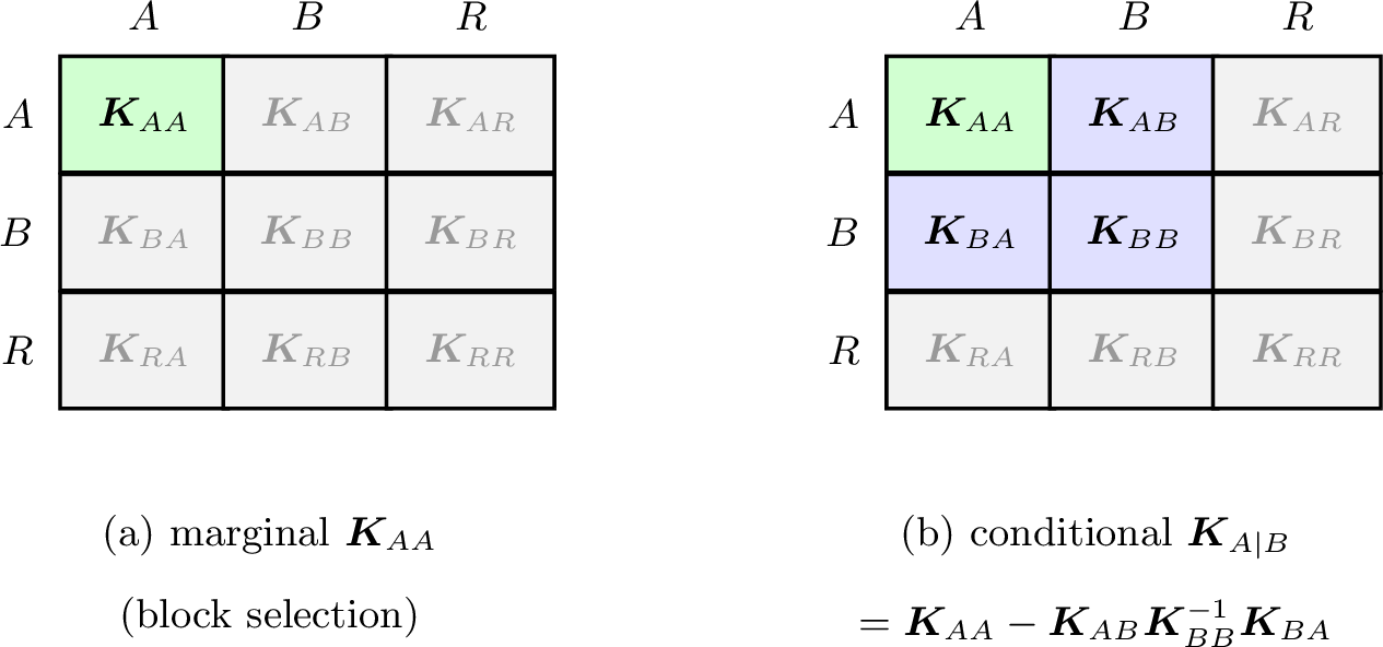
Because the K-recursion (2.3) has already produced every node-pair block \(\boldsymbol{K}_{jk}\), the set-indexed blocks used above are simply gathered from it (\(\boldsymbol{K}_{AA}\) stacks the blocks \(\boldsymbol{K}_{jk}\) with \(j,k\in A\), and \(\boldsymbol{K}_{AB},\boldsymbol{K}_{BB}\) likewise), so no per-query recomputation is needed. 1 reads the two formulas off this assembled matrix. In panel (a) the marginal of \(V_A\) is the green diagonal block \(\boldsymbol{K}_{AA}\). In panel (b) the posterior covariance \(\boldsymbol{K}_{A\mid B}\) combines the anchor block \(\boldsymbol{K}_{AA}\) (green) with the blocks \(\boldsymbol{K}_{AB},\boldsymbol{K}_{BA}\) that couple the query to the observation and the observed block \(\boldsymbol{K}_{BB}\) (blue); the unrelated nodes \(R\) (grey) are dropped. Conditioning therefore shrinks \(\boldsymbol{K}_{AA}\) by exactly the information that the observation \(B\) carries about \(A\).

Every inference quantity in this paper is built the same way, from a handful of operations on sub-blocks of the one matrix \(\boldsymbol{K}\): block selection (marginals, 5 ), the Schur complement (conditioning, 7 ), the log-determinant of a block (entropies, mutual information, and Gaussian log-likelihoods, 3.3), and the linear solve \(\boldsymbol{K}_{BB}^{-1}(\cdot)\) (posterior means and node-wise regressions). We call this block algebra on the covariance chart. The chart supplies the object and the four primitives the operations; together they constitute the covariance calculus of the title, and [sec:conditioning] [sec:mi] develop it for the basic queries.

Two properties make this the organizing principle of the paper. First, each operation is a smooth map (evaluated in practice by one Cholesky factorization per solve and log-determinant), so composing it with the chart \(\Phi_{\mathcal{G}}:\boldsymbol{\eta}\mapsto\boldsymbol{K}\) makes any inference quantity a single differentiable function of the learnable parameters \(\boldsymbol{\eta}\); one reverse-mode AD sweep then returns its gradient with respect to every entry of \(\boldsymbol{\eta}\), with no query- or topology-specific derivation. Second, the same operations, over the same chart, drive the later sections: a marginal log-likelihood is a log-determinant plus a trace (4); the Fisher information is built from derivatives of an observed block \(\boldsymbol{K}_{\mathcal{O}\mathcal{O}}\) (5). A query that conditions on, or takes the density of, a node set requires the corresponding block of \(\boldsymbol{K}\) to be positive definite (4).

3.2 Marginalization and Conditioning↩︎

We now record the two basic queries of 3.1 in the form used by the rest of the paper.

Marginalization. For a query set \(A\), the marginal law is \[V_A\sim\mathcal{N}(\boldsymbol{0},\boldsymbol{K}_{AA}), \label{eq:marginal}\tag{8}\] whose covariance is the diagonal block \(\boldsymbol{K}_{AA}\), read off the blocks of 2.3 with no further computation.

Conditioning. Let \(B\) be an observed set with \(\boldsymbol{K}_{BB}\succ\boldsymbol{0}\). Given \(V_B=\boldsymbol{b}\), the query \(V_A\) is Gaussian with \[\begin{align} \mathbb{E}[V_A\mid V_B=\boldsymbol{b}] &= \boldsymbol{K}_{AB}\boldsymbol{K}_{BB}^{-1}\boldsymbol{b}, \tag{9}\\ \mathop{\mathrm{Cov}}[V_A\mid V_B] &= \boldsymbol{K}_{A\mid B} =\boldsymbol{K}_{AA}-\boldsymbol{K}_{AB}\boldsymbol{K}_{BB}^{-1}\boldsymbol{K}_{BA}. \tag{10} \end{align}\] The posterior mean 9 is the minimum-mean-square-error estimate of \(V_A\) from the observation \(\boldsymbol{b}\) and is linear in \(\boldsymbol{b}\); although the model is zero-mean, conditioning on a specific value yields this nonzero data-driven mean. The posterior covariance 10 , by contrast, does not depend on \(\boldsymbol{b}\): the observed value relocates the distribution, but the reduction in uncertainty is fixed by the model alone.

The condition \(\boldsymbol{K}_{BB}\succ\boldsymbol{0}\) is the density-level requirement of 4: it is what makes \(\boldsymbol{K}_{BB}^{-1}\), and hence the conditional law, well-defined, and it holds automatically whenever the observed nodes carry a positive-definite innovation. Numerically we never form \(\boldsymbol{K}_{BB}^{-1}\). A Cholesky factor \(\boldsymbol{K}_{BB}=\boldsymbol{L}\boldsymbol{L}^{\mathsf{T}}\) is computed once; the gain \(\boldsymbol{K}_{AB}\boldsymbol{K}_{BB}^{-1}\) and the mean 9 follow from triangular solves against \(\boldsymbol{L}\), and the Schur complement 10 is re-symmetrized as \(\tfrac12(\boldsymbol{K}_{A\mid B}+\boldsymbol{K}_{A\mid B}^{\mathsf{T}})\) to discard the antisymmetric part introduced by finite-precision arithmetic. The log-determinants of the information measures in 3.3 are evaluated by the same Cholesky route.

3.3 Mutual Information and Conditional Independence↩︎

The information measures follow from the same conditional covariances by a log-determinant [18]. For disjoint node sets \(A,B,C\), the mutual information and the conditional mutual information (CMI) are \[\begin{align} I(V_A;V_B) &= \tfrac12\big(\log\det\boldsymbol{K}_{AA}-\log\det\boldsymbol{K}_{A\mid B}\big), \tag{11}\\ I(V_A;V_B\mid V_C) &= \tfrac12\big(\log\det\boldsymbol{K}_{A\mid C} -\log\det\boldsymbol{K}_{A\mid BC}\big), \tag{12} \end{align}\] in nats, where each conditional covariance \(\boldsymbol{K}_{A\mid\cdot}\) is the Schur complement of 10 ; for circular-complex networks the factor \(\tfrac12\) becomes \(1\) (3). Both measures require the conditioned blocks to be positive definite (4), and both are evaluated from Cholesky log-determinants of blocks already assembled in 3.2.

Because \(\boldsymbol{K}\) is a smooth function of \(\boldsymbol{\eta}\), so are 11 and 12 ; the differentiable optimization of the mutual information over the controllable parameters is the subject of the companion paper [3], with conditional-mutual-information objectives for multi-terminal networks in [5]. Here the CMI serves instead as a test of conditional independence: for jointly Gaussian variables, \[V_A\perp V_B\mid V_C \iff I(V_A;V_B\mid V_C)=0, \label{eq:ci}\tag{13}\] which holds exactly when the conditional cross-covariance \(\boldsymbol{K}_{AB\mid C}=\boldsymbol{K}_{AB}-\boldsymbol{K}_{AC}\boldsymbol{K}_{CC}^{-1}\boldsymbol{K}_{CB}\) is the zero matrix. Testing conditional independence is therefore a zero-test on a single Schur-complement block. The test is a basic primitive in several roles: constraint-based structure learning queries exactly such a CI oracle, model diagnostics check the independences a hypothesized structure implies (for instance, whether a first-order Markov model suffices, 6.6), and a vanishing CMI certifies a sensor as redundant given those already selected, or an observable as leakage-free given the public variables.

Relation to the graph. Two notions of conditional independence should be kept apart. The test 13 is parameter-specific: it concerns the particular \(\boldsymbol{\eta}\) at hand. A structural independence, by contrast, holds for all parameter values and is read from the graph by d-separation [2], equivalently by trek separation [13] in the Gaussian case. A structural independence implies the numerical test 13 identically in \(\boldsymbol{\eta}\); the converse can fail only on a measure-zero set of parameters, where a CMI vanishes without a graphical reason. In the vector-valued setting the test is also finer-grained than the graph: d-separation is all-or-nothing at the node level, whereas a low-rank edge can leave \(\boldsymbol{K}_{AB\mid C}\) nonzero but rank-deficient, so that only certain linear combinations of \(V_A\) are conditionally independent of \(V_B\), a sub-block structure the Schur-complement test resolves and trek separation characterizes [13]. The K-recursion supplies the covariance blocks for the numerical test, complementing the graphical criterion.

3.4 Forward Sampling↩︎

The topological forward pass that propagates second moments in the K-recursion also draws samples from the network. Traversing the nodes in topological order, we simulate the structural equation 1 directly: at each node we draw a standard normal \(\boldsymbol{\xi}_j\sim\mathcal{N}(\boldsymbol{0},\boldsymbol{I}_{d_j})\) and set \[V_j=\sum_{i\in\mathrm{Pa}(j)}\boldsymbol{A}_{ji}V_i+\boldsymbol{L}_j\boldsymbol{\xi}_j, \label{eq:sample}\tag{14}\] where \(\boldsymbol{L}_j\) is any factor of the innovation covariance, \(\boldsymbol{\Sigma}_j=\boldsymbol{L}_j\boldsymbol{L}_j^{\mathsf{T}}\), so that \(\boldsymbol{L}_j\boldsymbol{\xi}_j\) realizes the innovation \(Z_j\) of 1 . One such pass produces one draw of the full vector \(V\sim\mathcal{N}(\boldsymbol{0},\boldsymbol{K})\), and \(N\) independent runs give \(N\) i.i.d.samples. A Cholesky factor serves when \(\boldsymbol{\Sigma}_j\succ\boldsymbol{0}\), and an eigendecomposition factor when \(\boldsymbol{\Sigma}_j\) is singular, so that a deterministic node (\(\boldsymbol{\Sigma}_j=\boldsymbol{0}\)) simply propagates its parents. The pass is linear in the size of the graph and, like the covariance recursion, forms neither \(\boldsymbol{K}\) nor any inverse: it realizes the joint law node by node.

Sampling is the generative counterpart of the inference queries above and the data source for the estimators of 4. The sample covariance of the draws converges to the analytic \(\boldsymbol{K}\) of 2.3, which both cross-checks the backend and enables Monte-Carlo evaluation of quantities that lack a closed form, for example nonlinear statistics of \(V\) or empirical mutual-information and estimator-variance studies. In the complex case the innovations are circularly symmetric (3).

4 Estimation↩︎

So far the parameters have been given, and the covariance chart has run forward, from \(\boldsymbol{\eta}\) to \(\boldsymbol{K}\) to the queries of 3. Estimation is the inverse problem: from data, recover the learnable parameters \(\boldsymbol{\eta}\) that generated it. We treat two regimes, full observation by maximum likelihood (4.1) and partial observation with hidden nodes by the marginal likelihood (4.2); both minimize one differentiable objective through the chart.

4.1 Full Observation: Maximum Likelihood↩︎

From \(N\) independent realizations \(\boldsymbol{v}^{(1)},\dots,\boldsymbol{v}^{(N)}\) of the full node vector \(V\), form the sample covariance \[\hat{\boldsymbol{K}}=\frac{1}{N}\sum_{n=1}^{N}\boldsymbol{v}^{(n)}(\boldsymbol{v}^{(n)})^{\mathsf{T}}. \label{eq:samplecov}\tag{15}\] Up to an additive constant and a positive factor, the negative log-likelihood is \[L(\boldsymbol{\eta})=\log\det\boldsymbol{K}+\mathop{\mathrm{tr}}\!\big(\boldsymbol{K}^{-1}\hat{\boldsymbol{K}}\big), \label{eq:nll}\tag{16}\] a function of the parameters through the covariance chart \(\boldsymbol{\eta}\mapsto\boldsymbol{K}\); the maximum-likelihood estimate is exactly its minimizer, \(\hat{\boldsymbol{\eta}}=\arg\min_{\boldsymbol{\eta}}L(\boldsymbol{\eta})\). This objective is natural on two counts. First, maximum likelihood is consistent and asymptotically efficient. Second, it is a Kullback–Leibler projection: minimizing \(L\) is the same as minimizing the divergence \(\mathrm{KL}\big(\mathcal{N}(\boldsymbol{0},\hat{\boldsymbol{K}})\,\|\,\mathcal{N}(\boldsymbol{0},\boldsymbol{K})\big)\), so the estimate is the covariance closest to the empirical \(\hat{\boldsymbol{K}}\) within the family the DAG can realize.

Since that chart is a differentiable computation graph (2.3), so is \(L\): one reverse-mode AD sweep returns the exact gradient \(\nabla_{\boldsymbol{\eta}}L\), propagated through both the K-recursion and the construction of the edges from \(\boldsymbol{\eta}\), so \(L\) is minimized by gradient descent in a positive-definite-preserving parametrization, with no per-node or per-topology gradient derivation. One caveat is in order: \(L\) is convex in the precision \(\boldsymbol{K}^{-1}\) but not, in general, in \(\boldsymbol{\eta}\), since the chart is polynomial. With free per-node parameters the full-observation MLE is available in closed form by node-wise regression, but under the tied, structured, or hidden-node parametrizations of interest here, gradient descent is guaranteed a stationary point only; random initializations sufficed in 6, and the Fisher analysis of 5 flags the flat gauge directions along which minimizers form orbits. This is the estimator the framework provides; unchanged, it handles hidden nodes (4.2) and any structured parametrization of the edges (2.2).

A nonzero data mean, when present, is removed by centering before forming 15 , which leaves 16 unchanged (2).

4.2 Partial Observation: Marginal Likelihood↩︎

In many networks not every node can be measured. A hidden common cause, an unmeasured relay or state node, or a latent factor is seen only through its effect on the rest of the network. Writing \(\mathcal{O}\) for the observed nodes, we must recover \(\boldsymbol{\eta}\) from data on \(\mathcal{O}\) alone. The difficulty is statistical rather than procedural: a hidden node cannot be fitted by its own regression, and marginalizing it out couples the observed nodes, so no node-wise closed form survives. On the chart, however, marginalization is mere block selection (3.2), and the estimator is the one of 4.1 unchanged: minimize the likelihood of the observed subvector by gradient descent.

Since \(V_\mathcal{O}\sim\mathcal{N}(\boldsymbol{0},\boldsymbol{K}_{\mathcal{O}\mathcal{O}})\), the observed-data negative log-likelihood is, up to an additive constant and a positive factor, \[L(\boldsymbol{\eta})=\log\det\boldsymbol{K}_{\mathcal{O}\mathcal{O}} +\mathop{\mathrm{tr}}\!\big(\boldsymbol{K}_{\mathcal{O}\mathcal{O}}^{-1}\boldsymbol{S}\big), \label{eq:marglik}\tag{17}\] where \(\boldsymbol{S}\) is the sample covariance of the observed nodes and \(\boldsymbol{K}_{\mathcal{O}\mathcal{O}}\) is the observed block of \(\boldsymbol{K}\) from the K-recursion. This is 16 restricted to \(\mathcal{O}\); with per-sample missing data it averages the per-pattern terms \(\log\det\boldsymbol{K}_{O_nO_n}+\boldsymbol{y}_n^{\mathsf{T}}\boldsymbol{K}_{O_nO_n}^{-1}\boldsymbol{y}_n\) over the patterns, where \(O_n\) and \(\boldsymbol{y}_n\) are the observed set and observed values of sample \(n\). Forming \(\boldsymbol{K}_{\mathcal{O}\mathcal{O}}\) with its Cholesky log-determinant and solve costs \(O(D_\mathcal{O}^3)\) in the observed dimension \(D_\mathcal{O}=\sum_{j\in\mathcal{O}}d_j\), and one AD sweep through the K-recursion again returns the exact gradient \(\nabla_{\boldsymbol{\eta}}L\), for any parametrization including the tied and structured parameters of 1. This direct route complements expectation–maximization [12] rather than replacing it: where closed-form E- and M-steps exist, EM remains effective, but every tied or structured parametrization requires its own M-step derivation, whereas 17 is differentiated through the covariance chart with no such per-parametrization work.

5 Identifiability and Reliability↩︎

Estimation raises two further questions: identifiability, whether \(\boldsymbol{\eta}\) can be recovered from the observed nodes at all or whether different parameters produce the same observed distribution, and reliability, how precisely an identifiable \(\boldsymbol{\eta}\) can be estimated, that is, how much the estimate scatters around the truth. Both are answered by one object, the Fisher information, which measures how sensitively the observed distribution responds to a change in \(\boldsymbol{\eta}\); a direction of \(\boldsymbol{\eta}\) that barely moves the distribution is hard to estimate, and one that moves it sharply is easy. 5.1 constructs this metric on the covariance chart, and 5.2 reads local identifiability off its rank and Cramér–Rao reliability off its inverse.

5.1 The Pullback (Slepian–Bangs) Fisher Metric↩︎

Because the observed nodes are zero-mean Gaussian, \(V_\mathcal{O}\sim\mathcal{N}(\boldsymbol{0},\boldsymbol{K}_{\mathcal{O}\mathcal{O}})\), all of that sensitivity is carried by how the observed covariance moves with \(\boldsymbol{\eta}\). Identify \(\boldsymbol{\eta}\) with the real vector \((\eta_1,\dots,\eta_q)^{\mathsf{T}}\) of its \(q\) free scalar coordinates: by 2.2 these are exactly the parameters to be estimated, whereas any fixed, known factors (a known channel, a fixed structure) enter \(\boldsymbol{K}_{\mathcal{O}\mathcal{O}}\) only as constants and are held fixed in the derivatives below.

Recall the general definitions. For a parametric family of densities \(p_{\boldsymbol{\eta}}\), the per-observation Fisher information matrix is the covariance of the score, \(G_{ab}(\boldsymbol{\eta})=\mathbb{E}[s_a s_b]\), where \(s_c=\partial\log p_{\boldsymbol{\eta}}(v)/\partial\eta_c\) is the score with respect to the \(c\)th coordinate. Information geometry reads \(G\) as a Riemannian metric on the parameter space, the Fisher–Rao metric [16]: between neighboring models, \(\mathrm{KL}\big(p_{\boldsymbol{\eta}}\,\|\,p_{\boldsymbol{\eta}+\boldsymbol{\delta}}\big) =\tfrac12\boldsymbol{\delta}^{\mathsf{T}}G(\boldsymbol{\eta})\boldsymbol{\delta} +o(\lVert\boldsymbol{\delta}\rVert^{2})\), so \(G\) is exactly the local distinguishability of parameters from data. For the zero-mean Gaussian family at hand the parameters enter only through \(\boldsymbol{K}_{\mathcal{O}\mathcal{O}}\), and the expectation evaluates in closed form, giving the per-observation Fisher metric \(G=(G_{ab})\in\mathbb{R}^{q\times q}\) on the parameters, whose \((a,b)\) entry is \[G_{ab}(\boldsymbol{\eta})=\tfrac12\,\mathop{\mathrm{tr}}\!\Big[ \boldsymbol{K}_{\mathcal{O}\mathcal{O}}^{-1}\frac{\partial\boldsymbol{K}_{\mathcal{O}\mathcal{O}}}{\partial\eta_a}\, \boldsymbol{K}_{\mathcal{O}\mathcal{O}}^{-1}\frac{\partial\boldsymbol{K}_{\mathcal{O}\mathcal{O}}}{\partial\eta_b}\Big], \label{eq:fisher}\tag{18}\] for \(a,b\in\{1,\dots,q\}\): the Slepian–Bangs formula [15], the closed form the general definition takes for a zero-mean Gaussian family (the factor \(\tfrac12\) becomes \(1\) in the circular-complex case, 3; 7.2 gives the derivation). Every ingredient comes from the K-recursion: \(\boldsymbol{K}_{\mathcal{O}\mathcal{O}}\) is a forward pass and its Jacobian \(\partial\boldsymbol{K}_{\mathcal{O}\mathcal{O}}/\partial\eta_a\) follows by automatic differentiation, one sweep per parameter, so \(G\) is obtained analytically, with no sampling, in \(O(q)\) AD sweeps. Since the derivative computation can itself be retained as part of the computation graph, the same construction also supports nested AD: smooth scalar criteria built from \(G\), such as Cramér–Rao design objectives based on \(G^{-1}\) or a regularized inverse, can be differentiated again with respect to the underlying parameters or design variables.

In this sense \(G\) is not a new model-specific object but the pullback of the Fisher–Rao metric of the Gaussian family along the covariance chart, summarizing exactly the parameter directions visible through the observed distribution. It is the common root of what follows (5.2): its rank decides identifiability and its (pseudo-)inverse bounds the estimation error.

5.2 Local Identifiability, Gauges, and Reliability↩︎

The parameters are locally identifiable from \(\mathcal{O}\) exactly when the Fisher metric has full rank, \(\mathop{\mathrm{rank}}G=q\), with \(q\) the number of parameters. A rank deficiency exposes a gauge: a null direction \(\boldsymbol{u}\) with \(G\boldsymbol{u}=\boldsymbol{0}\) is a change of \(\boldsymbol{\eta}\) that leaves \(\boldsymbol{K}_{\mathcal{O}\mathcal{O}}\), and hence the observed distribution, unchanged to first order. Motion along such a direction is invisible in the data, so the parameters it mixes cannot be told apart; \(\ker G\) is the tangent space of these gauge orbits, and its dimension \(q-\mathop{\mathrm{rank}}G\) counts the undetermined directions. Such a point is, in the terminology of statistical learning theory, a singular point of the model [17]: the map from parameters to distributions fails to be locally one-to-one, so distinct parameters realize the same observed law, as the following example shows exactly.

The canonical example is the latent scale gauge. Let a hidden node \(H\) of variance \(\sigma^2\) feed two observed nodes, \(Y_1=aH\) and \(Y_2=bH\). The observed covariance depends on \((a,b,\sigma^2)\) only through the products \(a^2\sigma^2\), \(b^2\sigma^2\), and \(ab\,\sigma^2\), so the reparametrization \((a,b,\sigma^2)\mapsto(a/t,\,b/t,\,t^2\sigma^2)\) leaves \(\boldsymbol{K}_{\mathcal{O}\mathcal{O}}\) invariant for every \(t\neq0\). Its generator lies in \(\ker G\): the latent scale is unidentifiable, and only gauge-invariant combinations (here \(a\sigma\) and \(b\sigma\)) can be recovered. Reporting \(\mathop{\mathrm{rank}}G\), the smallest eigenvalues of \(G\) (which flag near-degeneracy), and the null eigenvectors mapped back to the parameters therefore diagnoses exactly which parameters, or which combinations, the observed nodes leave undetermined. In numerical use this verdict is read from the spectrum of \(G\) rather than by an exact symbolic rank test: exact zeros mark gauges of the covariance chart, whereas small but nonzero eigenvalues mark near-gauges, with correspondingly large Cramér–Rao standard errors.

The same metric also quantifies how well the identifiable parameters can be estimated. Since \(G\) is the per-observation Fisher information, the Cramér–Rao bound states that any unbiased estimator \(\hat{\boldsymbol{\eta}}\) obeys \[\mathop{\mathrm{Cov}}(\hat{\boldsymbol{\eta}})\succeq G^{-1}. \label{eq:crb}\tag{19}\] The maximum-likelihood estimator of 4 attains this bound asymptotically: for \(N\) independent observations its error covariance approaches \(\tfrac1N G^{-1}\), so standard errors shrink as \(1/\sqrt{N}\). The per-parameter standard errors are the square roots of the diagonal of \(G^{-1}\), obtained analytically from the K-recursion Jacobian with no Monte Carlo; because they are read from the diagonal of the full inverse, each already accounts for jointly estimating the remaining parameters rather than treating them as known.

When \(G\) is rank-deficient (a gauge, as above), the bound is infinite along \(\ker G\): a parameter whose unit vector has a component in the null space has unbounded variance and is flagged non-identifiable, with an infinite standard error, while on the identifiable subspace the bound is the Moore–Penrose pseudo-inverse of \(G\) and its diagonal gives finite standard errors. One Fisher object thus serves both roles at once: its null space is the identifiability verdict, and its (pseudo-)inverse is the reliability of the estimates.

6 Numerical Experiments↩︎

We exercise the whole framework on two examples: a linear Gaussian state-space model (a first-order vector autoregression observed in noise), whose chain structure admits validation against the classical Kalman recursions, and a skip-connected extension of the same model, whose merging nodes make the parent cross-covariances essential (6.6). The purpose is validation rather than application benchmarking: each task carries either a classical reference computation or a Monte-Carlo quantity against which the covariance-chart result is checked. All numbers below are produced by the reference implementation; where a closed form exists, we report the agreement with it. The exact fitting settings and seeds are recorded in 7.3.

6.1 Setup↩︎

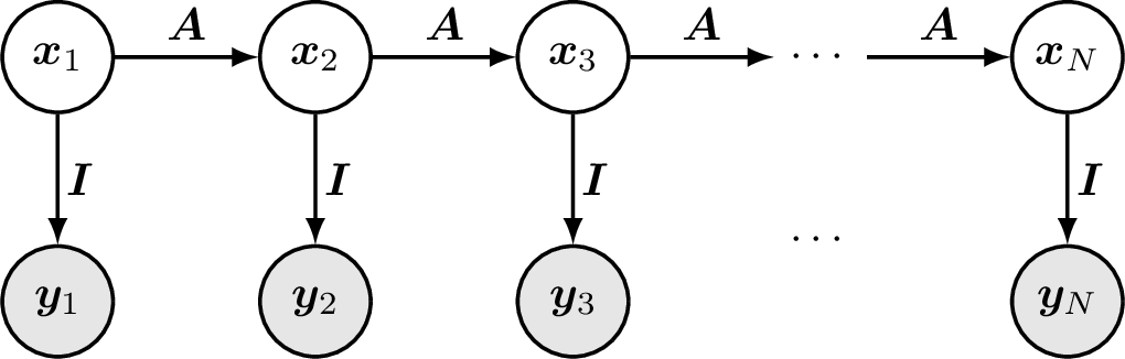
The model has \(d\)-dimensional latent states \(\boldsymbol{x}_1,\dots,\boldsymbol{x}_N\) and noisy observations \(\boldsymbol{y}_1,\dots,\boldsymbol{y}_N\), \[\boldsymbol{x}_n=\boldsymbol{A}\boldsymbol{x}_{n-1}+\boldsymbol{u}_n,\qquad \boldsymbol{y}_n=\boldsymbol{x}_n+\boldsymbol{w}_n, \label{eq:lds}\tag{20}\] with \(\boldsymbol{x}_1\sim\mathcal{N}(\boldsymbol{0},\boldsymbol{P}_0)\), process noise \(\boldsymbol{u}_n\sim\mathcal{N}(\boldsymbol{0},\boldsymbol{Q})\), and observation noise \(\boldsymbol{w}_n\sim\mathcal{N}(\boldsymbol{0},\boldsymbol{R})\), all independent; following state-space convention, these random vectors are written as boldface lowercase. As a Bayesian network (2) this is a \(2N\)-node DAG: the state chain \(\boldsymbol{x}_{n-1}\!\to\!\boldsymbol{x}_n\) carries the transition \(\boldsymbol{A}\), tied across every step, and each \(\boldsymbol{x}_n\!\to\!\boldsymbol{y}_n\) carries the identity. The transition is itself structured as \(\boldsymbol{A}=\boldsymbol{S}\boldsymbol{T}\) with \(\boldsymbol{S}\) a fixed, known matrix and \(\boldsymbol{T}\) the learnable parameter, a concrete instance of the tied/structured parametrization of 1. We take \(d=2\), \(N=8\), \(\boldsymbol{S}=\left[\begin{smallmatrix}1&0.5\\0&1\end{smallmatrix}\right]\), \(\boldsymbol{T}=\left[\begin{smallmatrix}0.4&-0.6\\0.2&0.6\end{smallmatrix}\right]\) (so \(\boldsymbol{A}=\left[\begin{smallmatrix}0.5&-0.3\\0.2&0.6\end{smallmatrix}\right]\), with spectral radius \(0.6\)), \(\boldsymbol{P}_0=\boldsymbol{I}\), \(\boldsymbol{Q}=0.1\,\boldsymbol{I}\), and \(\boldsymbol{R}=0.2\,\boldsymbol{I}\). This is the chain special case in which the K-recursion reduces to the Kalman covariance recursion, which makes it an ideal validation target rather than a new method. Throughout this section \(M\) denotes the number of i.i.d.trajectories, each a realization of the full \(2N\)-node network; \(M\) plays the role of the sample count \(N\) of , since \(N\) here is reserved for the chain length.

6.2 Inference and Conditional Independence↩︎

The framework assembles the joint covariance by the K-recursion and answers each query by block algebra on it (3). We check three facts against the classical recursions. Prior state covariance: the marginal \(\mathop{\mathrm{Cov}}[\boldsymbol{x}_n]\) read from the chart matches the open-loop covariance recursion \(\boldsymbol{\Sigma}_n=\boldsymbol{A}\boldsymbol{\Sigma}_{n-1}\boldsymbol{A}^{\mathsf{T}}+\boldsymbol{Q}\) (the Kalman prediction step, applied with no measurement updates) to machine precision (maximum block error \(6.9\times10^{-18}\) over \(n\)), and \(\boldsymbol{\Sigma}_n\) approaches the fixed point of that recursion, the unique solution \(\bar{\boldsymbol{\Sigma}}\) of the discrete Lyapunov (Stein) equation \(\bar{\boldsymbol{\Sigma}}=\boldsymbol{A}\bar{\boldsymbol{\Sigma}}\boldsymbol{A}^{\mathsf{T}}+\boldsymbol{Q}\), equivalently \(\bar{\boldsymbol{\Sigma}}=\sum_{k=0}^{\infty}\boldsymbol{A}^{k}\boldsymbol{Q}(\boldsymbol{A}^{\mathsf{T}})^{k}\), which exists because the spectral radius of \(\boldsymbol{A}\) is \(0.6<1\); at \(n=N=8\) the gap is \(\lVert\boldsymbol{\Sigma}_N-\bar{\boldsymbol{\Sigma}}\rVert=9.6\times10^{-4}\). Smoothing: conditioning the states on all observations, \(\mathop{\mathrm{Cov}}[\boldsymbol{x}_n\mid \boldsymbol{y}_{1:N}]\), is the Schur complement 10 ; it matches the Rauch–Tung–Striebel smoother covariance to \(1.5\times10^{-16}\). Conditioning on the observations is therefore exactly Kalman smoothing, obtained here as a special case of 3.2. Conditional independence: the Markov property surfaces as a vanishing CMI. For a representative triple, \(I(\boldsymbol{x}_{n-1};\boldsymbol{x}_{n+1}\mid \boldsymbol{x}_n)\) evaluates to exactly zero in double precision, as 13 predicts, whereas conditioning off the separating node leaves the two states dependent, \(I(\boldsymbol{x}_{n-1};\boldsymbol{x}_{n+1}\mid \boldsymbol{x}_{n+2})=0.156\) nats.

6.3 Forward Sampling↩︎

Drawing trajectories by the forward pass of 3.4 and forming the sample covariance reproduces the analytic \(\boldsymbol{K}\): the relative error \(\lVert\hat{\boldsymbol{K}}-\boldsymbol{K}\rVert/\lVert\boldsymbol{K}\rVert\) is \(7.4\times10^{-2}\), \(3.4\times10^{-2}\), \(7.1\times10^{-3}\), \(2.7\times10^{-3}\) at \(M=10^{3},10^{4},10^{5},10^{6}\) trajectories, the \(1/\sqrt{M}\) Monte-Carlo rate.

6.4 Estimation of the Tied Factor↩︎

The data are \(M=2\times10^{5}\) trajectories drawn from the true model of 6.1 by the forward sampling of 6.3; the hidden states are then discarded, so the estimator sees only the observations \(\boldsymbol{y}_{1:N}\) of each trajectory. From these observations alone, and starting from a random initialization, we estimate the shared factor \(\boldsymbol{T}\) by minimizing the negative marginal log-likelihood 17 through the differentiable chart, with \(\boldsymbol{A}=\boldsymbol{S}\boldsymbol{T}\) tied across all \(N-1\) transitions; the true \(\boldsymbol{T}\) enters only the data generation and the final error evaluation. The negative log-likelihood falls from \(5.99\) to \(0.99\) and the estimate recovers the truth, \(\lVert\hat{\boldsymbol{T}}-\boldsymbol{T}\rVert=8.5\times10^{-4}\) (and \(\lVert\hat{\boldsymbol{A}}-\boldsymbol{A}\rVert=7.4\times10^{-4}\)): a single \(2\times2\) factor is identified from the whole trajectory ensemble, with the gradient accumulated over its shared occurrences by one AD sweep (1).

6.5 Identifiability and Reliability↩︎

The Slepian–Bangs Fisher information over \(\boldsymbol{T}\) (a \(q=4\) parameter vector), pulled back through \(\boldsymbol{T}\mapsto\boldsymbol{K}_{\mathcal{O}\mathcal{O}}\) 18 , has full rank \(4\) with eigenvalues \(\{4.6,6.7,13.2,17.0\}\), so \(\boldsymbol{T}\) is locally identifiable from the observations (5.2), and its inverse sets the reliability of the estimator. Over \(400\) Monte-Carlo trials at each sample size \(M\), the empirical standard deviation of the maximum-likelihood estimate tracks the analytic Cramér–Rao standard error \(\sqrt{\operatorname{diag}((MG)^{-1})}\) and follows the \(1/\sqrt{M}\) law (3). At \(M=2000\) the (analytic, empirical) per-parameter standard errors are \((8.7,8.9)\), \((8.4,8.3)\), \((7.5,7.4)\), and \((7.0,7.0)\) for \(T_{11},T_{12},T_{21},T_{22}\) respectively, in units of \(10^{-3}\): the analytic bound predicts the observed estimator scatter to within the Monte-Carlo error.

6.6 Beyond the Chain: Skip Connections↩︎

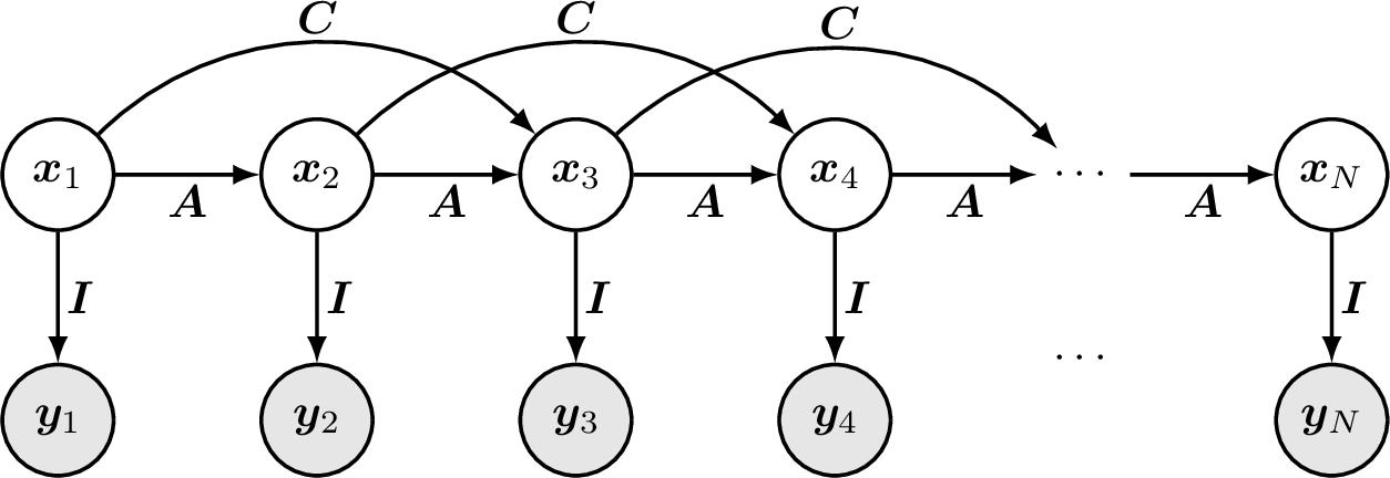
The second experiment takes the running example beyond the chain: a tied skip connection is added to 20 , \[\boldsymbol{x}_n=\boldsymbol{A}\boldsymbol{x}_{n-1}+\boldsymbol{C}\boldsymbol{x}_{n-2}+\boldsymbol{u}_n,\qquad n\geq3, \label{eq:skip}\tag{21}\] with the \(n=2\) step unchanged from 20 , \(\boldsymbol{A}=\boldsymbol{S}\boldsymbol{T}\) and all other settings as in 6.1, and the known skip matrix \(\boldsymbol{C}=\left[\begin{smallmatrix}0.15&0\\0.05&0.1\end{smallmatrix}\right]\) shared across all skip edges (4). Every state with \(n\geq3\) now merges two correlated parents, so the parent cross-covariances in the self-blocks of 4 become essential and the first-order recursions of 6.2 no longer apply to the graph as given; the classical route is a per-model reformulation, stacking \((\boldsymbol{x}_n,\boldsymbol{x}_{n-1})\) into a first-order companion state. The framework needs no such reformulation: the chart is simply re-run on the extended graph, and its marginals \(\mathop{\mathrm{Cov}}[\boldsymbol{x}_n]\) agree with the hand-augmented companion-form prediction recursion to machine precision (maximum error \(8.6\times10^{-17}\)).

The information queries track the new structure. The first-order Markov CMI, which vanished in 6.2, is now \(I(\boldsymbol{x}_{n-1};\boldsymbol{x}_{n+1}\mid\boldsymbol{x}_n)=0.023\) nats, since the skip edge keeps a path open around the conditioned node, while the second-order CMI \(I(\boldsymbol{x}_{n-1};\boldsymbol{x}_{n+2}\mid\boldsymbol{x}_n,\boldsymbol{x}_{n+1})\) is zero to double precision, exactly as d-separation predicts on 4.

The estimation and reliability pipeline then runs unchanged. Repeating 6.4 verbatim on the extended graph, with the states hidden and \(M=2\times10^{5}\) trajectories, the tied factor is recovered from a random initialization to \(\lVert\hat{\boldsymbol{T}}-\boldsymbol{T}\rVert=5.5\times10^{-4}\); the Fisher metric over \(\boldsymbol{T}\) retains full rank \(4\), and at \(M=2000\) the analytic Cramér–Rao standard errors \((7.5,7.3,6.6,6.2)\), in units of \(10^{-3}\), match the empirical scatter \((7.7,7.8,6.8,6.4)\) of \(400\) maximum-likelihood trials. The same metric also prices observation patterns with no further derivation: observing only the odd-indexed half of the sensors (the observation nodes), \(\boldsymbol{y}_1,\boldsymbol{y}_3,\boldsymbol{y}_5,\boldsymbol{y}_7\), keeps \(\boldsymbol{T}\) identifiable (again full rank) but inflates the bound to \((10.0,9.6,8.5,7.9)\), matched by the empirical \((10.1,10.1,8.6,7.7)\). 5 overlays the two \(95\%\) ellipses with their estimate clouds, the counterpart of 3 (b) on the extended graph: the cost of halving the sensors is read off analytically, before any data are collected. Nothing in the code or the derivations refers to the topology: the same chart, likelihood, and Fisher pullback serve the chain and its skip-connected extension alike.

7 Conclusion↩︎

We have developed inference, estimation, and identifiability for linear Gaussian Bayesian networks as one differentiable covariance calculus on a single backend, the K-recursion covariance chart \(\Phi_{\mathcal{G}}:\boldsymbol{\eta}\mapsto\boldsymbol{K}\). Every operation reduces to block algebra on the covariance it produces (block selection, a Schur complement, a log-determinant, and a linear solve): marginals and conditionals, mutual information and conditional-independence tests, forward sampling, maximum-likelihood estimation under full and partial (hidden-node) observation, and the Slepian–Bangs Fisher information with the local identifiability and Cramér–Rao reliability it induces. Because the chart is a smooth computation graph, automatic differentiation supplies every gradient in one backward sweep, over arbitrary vector-valued DAGs and arbitrary (including tied and structured) parametrizations, with no per-query or per-topology derivation. On a linear Gaussian state-space running example the framework reproduces the Kalman filter and Rauch–Tung–Striebel smoother to machine precision, certifies the Markov conditional independences as vanishing conditional mutual informations, recovers a tied transition factor from noisy observations of hidden states, and yields an analytic Cramér–Rao bound that matches the empirical scatter of the maximum-likelihood estimator. On a skip-connected extension of the same example, whose merging nodes take the graph beyond the chain, the identical pipeline runs unchanged: the marginals match a hand-augmented companion-form recursion, the conditional mutual information tracks d-separation, and the tied factor is again recovered with Cramér–Rao-validated reliability.

The covariance map and its statistical ingredients are classical; the contribution is their differentiable, unified formulation, realized in an open-source reference implementation. The same backend drives mutual-information optimization in a companion paper [3]. Natural extensions include intervention and formal observation design on the same chart, and a symbolic evaluation of the recursion for machine-checked proofs of conditional independence and identifiability.

The derivation of the K-recursion itself is given in the companion paper [3]. This appendix proves the two identities the paper rests on, the log-determinant information formulas and the Slepian–Bangs pullback, and records the settings behind the numbers of 6.

7.1 Log-Determinant Identities 11 –13↩︎

The differential entropy of a real Gaussian vector \(V_A\sim\mathcal{N}(\boldsymbol{0},\boldsymbol{K}_{AA})\) is \(h(V_A)=\tfrac12\log\det(2\pi e\,\boldsymbol{K}_{AA})\) [18]. Because the conditional covariance 10 does not depend on the observed value, the conditional entropy is \(h(V_A\mid V_B)=\tfrac12\log\det(2\pi e\,\boldsymbol{K}_{A\mid B})\), and \(I(V_A;V_B)=h(V_A)-h(V_A\mid V_B)\) gives 11 , the \(2\pi e\) factors canceling. Conditioning every entropy on \(V_C\) gives 12 .

For 13 , condition the pair \((V_A,V_B)\) on \(V_C\): the joint conditional covariance has diagonal blocks \(\boldsymbol{K}_{A\mid C},\boldsymbol{K}_{B\mid C}\) and off-diagonal block \(\boldsymbol{K}_{AB\mid C}\), and conditioning further on \(V_B\) gives the nested Schur complement \(\boldsymbol{K}_{A\mid BC} =\boldsymbol{K}_{A\mid C}-\boldsymbol{K}_{AB\mid C}\boldsymbol{K}_{B\mid C}^{-1}\boldsymbol{K}_{BA\mid C}\). Substituting into 12 , \[I(V_A;V_B\mid V_C)=-\tfrac12\log\det\!\big(\boldsymbol{I}-\boldsymbol{R}\boldsymbol{R}^{\mathsf{T}}\big), \label{eq:cmi95cc}\tag{22}\] with \(\boldsymbol{R}=\boldsymbol{K}_{A\mid C}^{-1/2}\boldsymbol{K}_{AB\mid C}\boldsymbol{K}_{B\mid C}^{-1/2}\). The singular values \(\rho_i\) of \(\boldsymbol{R}\) are the canonical correlations of \(V_A\) and \(V_B\) given \(V_C\) and lie in \([0,1)\), so \(I(V_A;V_B\mid V_C)=-\tfrac12\sum_i\log(1-\rho_i^2)\geq0\), with equality if and only if every \(\rho_i=0\), that is, \(\boldsymbol{K}_{AB\mid C}=\boldsymbol{0}\). This proves 13 , and nonnegativity along the way. In the circular-complex case the entropy is \(\log\det(\pi e\,\boldsymbol{K})\), which is where the factor \(\tfrac12\) of 11 –12 becomes \(1\) (3).

7.2 The Slepian–Bangs Pullback 18↩︎

Write \(\boldsymbol{K}\equiv\boldsymbol{K}_{\mathcal{O}\mathcal{O}}(\boldsymbol{\eta})\succ\boldsymbol{0}\) (4) and \(\partial_a\equiv\partial/\partial\eta_a\). The log-density of one observation \(v\sim\mathcal{N}(\boldsymbol{0},\boldsymbol{K})\) is \(\log p(v)=-\tfrac12\log\det(2\pi\boldsymbol{K})-\tfrac12 v^{\mathsf{T}}\boldsymbol{K}^{-1}v\). The matrix identities \(\partial_a\log\det\boldsymbol{K}=\mathop{\mathrm{tr}}(\boldsymbol{K}^{-1}\partial_a\boldsymbol{K})\) and \(\partial_a\boldsymbol{K}^{-1}=-\boldsymbol{K}^{-1}(\partial_a\boldsymbol{K})\boldsymbol{K}^{-1}\) give the score in centered quadratic-form shape, \[s_a(v)=\tfrac12\big(v^{\mathsf{T}}\boldsymbol{W}_a v-\mathop{\mathrm{tr}}(\boldsymbol{W}_a\boldsymbol{K})\big), \quad \boldsymbol{W}_a=\boldsymbol{K}^{-1}(\partial_a\boldsymbol{K})\boldsymbol{K}^{-1}, \label{eq:score}\tag{23}\] using \(\mathbb{E}[v^{\mathsf{T}}\boldsymbol{W}_a v]=\mathop{\mathrm{tr}}(\boldsymbol{W}_a\boldsymbol{K})\). Each \(\boldsymbol{W}_a\) is symmetric, and for a zero-mean Gaussian the covariance of two quadratic forms is \(\mathop{\mathrm{Cov}}(v^{\mathsf{T}}\boldsymbol{W}_a v,\,v^{\mathsf{T}}\boldsymbol{W}_b v) =2\mathop{\mathrm{tr}}(\boldsymbol{W}_a\boldsymbol{K}\boldsymbol{W}_b\boldsymbol{K})\) (Isserlis’ theorem). Hence \(G_{ab}=\mathbb{E}[s_a s_b]=\tfrac12\mathop{\mathrm{tr}}(\boldsymbol{W}_a\boldsymbol{K}\boldsymbol{W}_b\boldsymbol{K})\), and expanding \(\boldsymbol{W}_a,\boldsymbol{W}_b\), \[G_{ab}=\tfrac12\mathop{\mathrm{tr}}\!\big(\boldsymbol{K}^{-1}\partial_a\boldsymbol{K}\,\boldsymbol{K}^{-1}\partial_b\boldsymbol{K}\big),\] which is 18 . The parameters enter only through \(\boldsymbol{K}_{\mathcal{O}\mathcal{O}}\), so this is the Fisher information of the Gaussian family pulled back along \(\boldsymbol{\eta}\mapsto\boldsymbol{K}_{\mathcal{O}\mathcal{O}}\) by the chain rule, and the derivatives \(\partial_a\boldsymbol{K}_{\mathcal{O}\mathcal{O}}\) are exactly the AD Jacobian of the K-recursion. The same computation with the circular-complex density and the complex form of Isserlis’ theorem yields the factor \(1\) of 3.

7.3 Experimental Details↩︎

All numbers and figure data of 6 are produced by two scripts of the reference implementation, one per example, with fixed random seeds, so every reported digit is reproducible by one command each. Four settings deserve explicit mention. (i) In 6.4 the tied factor is estimated by minimizing the negative marginal log-likelihood 17 with Adam (learning rate \(0.02\), \(1500\) iterations) from a random initialization; the reported objective values are per-sample negative log-likelihoods up to the usual constant. (ii) In 6.5 each of the \(400\) trials per sample size draws \(M\) fresh trajectories, forms the observed sample covariance, and computes the maximum-likelihood estimate by Newton’s method on 17 (\(10\) iterations, gradient and Hessian by AD), initialized at the true parameter so that every trial converges to the consistent root of the likelihood equation, the standard practice when checking Cramér–Rao attainment. (iii) The Fisher matrix \(G\) of 18 is evaluated at the true parameter from the AD Jacobian, and the ellipse of 3 (b) is the \(95\%\) level set of the Gaussian whose covariance is the corresponding \(2\times2\) sub-block of \((MG)^{-1}\) at \(M=2000\). (iv) In 6.6 the tied factor is estimated with the same settings as (i), and the Monte-Carlo validation uses the same Newton procedure as (ii), with \(400\) trials of \(M=2000\) draws for each of the two observation patterns; the ellipses of 5 are constructed as in (iii).

Acknowledgment↩︎

This work was supported by JST, CRONOS, Japan Grant Number JPMJCS25N5.

References↩︎