Mean Time to Remediate Is Not a Fielding Model:
A Cadence Audit for Enterprise Vulnerability Management
July 05, 2026
Abstract
Enterprise security teams commonly summarize remediation through mean time to remediate (MTTR), SLA compliance, dwell time, or detection delay. These metrics are useful, but they can hide how fixes actually reach the estate: continuously, through scheduled maintenance windows, in deployment rings, or through emergency bypass paths. This paper introduces a remediation-cadence audit for enterprise vulnerability management. The audit records routine mean lag, release period, release fraction, cohort geometry, emergency/routine split, non-fielding delay, local residual-pressure evidence, and declared rate scenario. It compares a continuous same-mean shortcut with the recorded release calendar and reports a local capacity verdict plus a calendar discount: the fraction of mean-only local capacity consumed by calendarized fielding. Worked notional packets with the same 30-day mean lag show why this matters. Under the normalized screening scenario, a two-month release train consumes 17.4% of mean-only capacity, a monthly train 5.2%, and a two-week screen 1.3%; across a 16-fold attacker-adjustment rate band, the two-month discount remains at least about 12% and the monthly discount stays in the resolution-sensitive 3–8% range. The audit therefore turns cadence assessment into an evidence-resolution question: when the discount is material relative to residual-pressure uncertainty or claimed headroom, MTTR/SLA should not be used alone as fielding evidence. Release-geometry checks show that deployment rings do not automatically recover the continuous benchmark, and cohort staggering can help or hurt near capacity. The result is a reproducible governance diagnostic, not a breach predictor or CVE prioritizer.
Cybersecurity operations ,vulnerability management ,patch management , remediation metrics ,MTTR ,release cadence ,security governance , control validation
1 Introduction↩︎
A vulnerability-management dashboard can improve while the underlying fielding process becomes less safe to summarize. An enterprise security team may report lower mean time to remediate (MTTR), better SLA compliance, and shorter detection delay, while at the same time changing how defensive updates reach the estate: routine fixes are held for scheduled maintenance windows, assets move through deployment rings, and high-severity issues bypass the ordinary process. From a dashboard perspective the program looks healthier. From a security-operations perspective, however, the relevant question is different: is the reported mean lag still a safe representation of how defensive changes are actually fielded?
This paper studies that question as a remediation-cadence audit. The audit addresses a narrow but important reporting failure: MTTR, SLA compliance, MTTD, and dwell-time measures are useful governance indicators, but they are not fielding models. Two remediation processes can have the same reported mean lag while exposing the estate to different release geometry. One process may field changes continuously; another may wait for monthly, six-week, bimonthly, or quarterly release windows; another may clear only part of the eligible backlog at each window; and another may split emergency and routine fixes into different channels. The mean lag summarizes average timing. It does not say whether the release calendar itself changes the local security-governance conclusion.
The operational setting is familiar. Enterprise patch-management guidance treats remediation as a process of identifying, prioritizing, acquiring, installing, and verifying updates [1]. Public vendor and cloud documentation describes monthly security-update cycles, scheduled patching, maintenance configurations, and out-of-band update paths [2], [3]. CISA’s KEV catalog and current risk-based remediation directives illustrate exploited-vulnerability governance and remediation-deadline objects [4], [5]. Remediation measurement studies further show that vulnerability-remediation data can be skewed, long-tailed, and poorly summarized by a single mean [6]. These sources motivate the timing side of the audit. They do not, by themselves, say whether a mean remediation lag is a safe fielding representation for a local adaptive-risk claim.
The audit therefore records two kinds of evidence. The first is timing and fielding evidence: routine mean lag, release-window period, per-window release fraction, cohort phases or deployment rings, emergency-bypass rules, and a non-fielding delay budget for detection, validation, approval, testing, packaging, and other hard delays. The second is local residual-pressure evidence: an interval derived from BAS, red-team, purple-team, control-validation, postmortem, or expert-scored evidence for the audited channel. Public CVE, CVSS, EPSS, KEV, OSV, or advisory data can help define scope and prioritization, but they cannot replace local evidence about how the organization’s controls, detections, response processes, and compensating measures perform on the channel being audited [4], [7]–[9].
The audit returns a local capacity verdict and a calendar discount. A local channel is inside capacity when small disturbances in intended defensive posture, fielded defensive posture, and attacker technique share decay under the recorded remediation process. It is outside capacity when those disturbances grow from release window to release window: attacker adjustment outpaces the fielding of defensive changes on that channel. The calendar discount reports how much of the mean-only local capacity is consumed by the recorded release calendar under a declared local-channel rate scenario. This second output is crucial. It means the audit does not depend only on a sharp point estimate of residual pressure. If the discount is material relative to the claimed headroom, or if the residual-pressure evidence is too coarse to resolve the discount, the governance finding is that MTTR/SLA should not be used alone as fielding evidence.
The worked packets in this paper use a 30-day routine mean lag and a 15-day non-fielding delay budget. Under the normalized screening scenario used for the main calculations, a coarse two-month release train with full eligible backlog clearing consumes about 17.4% of mean-only local capacity. A monthly train with the same mean lag consumes about 5%. A shorter two-week screen consumes about 1.3%. Across the rate-scenario band checked in Section 6, the two-month discount remains at least about 12%, the monthly discount stays in the 3–8% resolution-sensitive band, and the two-week screen remains below 2%. These values change the interpretation of the worked example. The two-month packet gives a resolved cadence warning that remains visible under coarser evidence intervals. The monthly packet is still important because it is operationally common, but it is more resolution-sensitive: a binary inside/outside verdict requires sharper local residual-pressure evidence. The audit therefore reports not only whether a point estimate falls between two capacity boundaries, but also how much evidence resolution is needed before a mean-only fielding claim is defensible.
The release-geometry checks add two further operational findings. Splitting a monthly train into deployment rings at fixed per-asset cadence does not recover the continuous same-mean benchmark; it approaches a phase-averaged calendar process. Cohort staggering is also not automatically stabilizing near capacity: depending on the local channel and phase schedule, staggering can help or hurt. Thus rings and cohort phases should be recorded as audit fields rather than used as verbal assurance that staged rollout behaves like continuous fielding.
The technical backend extends an implementation-filter mechanism, but the contribution here is the security-operations audit built on top of it [10]. The paper contributes four elements. First, it formulates a remediation-cadence audit record that joins timing evidence, release geometry, emergency/routine channel separation, hard-delay budget, local residual-pressure evidence, and rate-scenario assumptions in one governance object. Second, it introduces calendar discount as a practical measure of how much capacity is consumed by calendarized fielding. Third, it uses notional but reproducible worked packets to show how the same reported mean lag can produce different evidence-resolution and capacity readings under different release calendars. Fourth, it validates release-geometry effects showing that rings do not automatically recover the continuous benchmark and that cohort phasing can change the local verdict near capacity.
The remainder of the paper follows the audit rather than the mathematical machinery. Section 2 defines the remediation-cadence workflow, audit record, output statuses, and calendar-discount interpretation. Section 3 gives worked notional audit packets and shows how calendar discount changes the management reading. Section 4 defines the calculation interface from an audit packet to capacity boundaries and discount. Section 5 explains why release windows create a calendar discount even when the mean lag is matched. Section 6 checks the finite thresholds, hard-delay placement checks, deployment rings, and cohort-phasing effects. The final sections position the audit relative to vulnerability-management and security measurement work, state limitations and responsible use, and summarize the implications for enterprise remediation reporting.
2 Remediation-cadence audit workflow↩︎
A remediation-cadence audit is a security-operations check for one question: when MTTR, SLA compliance, or a mean remediation lag is used as evidence that a local adaptive-risk channel is manageable, is the mean-only fielding representation adequate, or does the actual release calendar consume a material part of the available local capacity? The audit is not a general vulnerability-prioritization method. Its purpose is narrower: to decide whether the remediation calendar itself must be disclosed, tested, and governed as a security-relevant fielding variable.
The audit uses the terms inside capacity and outside capacity in an operational sense. A local channel is inside capacity when small disturbances in intended defensive posture, fielded defensive posture, and attacker technique share decay under the recorded remediation process. It is outside capacity when those disturbances grow from release window to release window: attacker adjustment outpaces the fielding of defensive changes on that channel. The verdict is therefore a local fielding-governance statement, not a forecast that a specific incident will occur.
The audit deliberately returns two outputs. The first is the familiar inside/outside capacity verdict obtained by comparing a local residual-pressure interval \(I_L=[L_-,L_+]\) with the mean-only and calendar-aware capacity boundaries. The second is the calendar discount \[\Delta_{\mathrm{cal}} = \frac{ L_{\mathrm{crit}}^{\mathrm{cont}} - L_{\mathrm{crit}}^{\mathrm{cal}} }{ L_{\mathrm{crit}}^{\mathrm{cont}} } . \label{eq:audit-calendar-discount}\tag{1}\] The discount is the fraction of mean-only local capacity consumed by the recorded release calendar. This number is reported even when the evidence for \(L\) is too coarse for a sharp inside/outside verdict. In practical terms, if a team’s claimed residual-pressure headroom is smaller than the calendar discount, then MTTR/SLA alone is not a safe fielding representation for that local claim. If the uncertainty in \(L\) is larger than the discount, the correct audit status is not a forced warning or a forced pass, but an input-resolution finding.
The discount should be interpreted under a declared local-channel rate scenario. The default calculation in this paper is a normalized screening convention in which local defensive-revision and attacker-adjustment rates are measured in units of the routine mean lag. A production audit should either declare that it is using this screening convention, supply local rate estimates, or run scenario bands over plausible rates. If the calendar discount is stable across the scenario band, the cadence finding is robust. If it is not stable, the audit should report a rate-scenario limitation rather than a sharp cadence verdict.
The audit should be run when the remediation process changes, or when the security claim being made depends on a mean lag rather than on fielding evidence. Typical triggers include migration from rolling deployment to monthly, six-week, bimonthly, or quarterly release trains; new change-freeze periods or approval gates; introduction of deployment rings or phase-shifted cohorts; emergency bypass being carved out of the routine path; SLA improvement accompanied by persistent incident, BAS, red-team, or control-validation pressure; BAS evidence that attacker activity is substituting toward techniques not yet covered by routine remediation; major endpoint, cloud, or application deployment tooling changes; and repeated exceptions to the nominal release calendar. The common feature is that MTTR may remain stable, or even improve, while the timing structure of defensive fielding has changed.
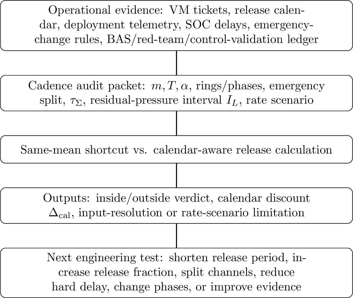
The audit record must be owned jointly. Vulnerability management usually owns MTTR, SLA reporting, remediation scope, ticket timing, and backlog evidence. Change management owns release-window policy, change-freeze rules, approval gates, and emergency-change procedures. Platform, endpoint, cloud, or application engineering owns deployment telemetry: release fractions, coverage curves, rings, phases, rollback rules, and effective fielded coverage. SOC and incident response own detection, triage, escalation, validation, and emergency response delays. BAS, red-team, purple-team, and control-validation teams provide evidence for the local residual-pressure ledger. Risk, governance, audit, or the CISO office owns the final interpretation, tolerance for uncertainty, and policy action. This ownership split matters because ticket closure is not necessarily fielded coverage, an approved emergency change is not necessarily deployed, and a written release policy is not evidence that production assets actually updated on that schedule.
Table 1 gives the minimum record. The record should be interval-first whenever possible. Instead of recording only \(L=2.70\), the analyst should record \(I_L=[L_-,L_+]\), the evidence used to produce it, and the owner who signed off on that evidence. The same principle applies to \(m\), \(T\), \(\alpha\), cohort phases, \(\tau_\Sigma\), and the local-channel rate scenario. If input uncertainty is larger than the calendar discount being tested, the correct output is an input-resolution finding, not a precise capacity claim.
| Field | Owner and evidence source | Purpose in the audit |
|---|---|---|
| Scope and local channel | Vulnerability management; asset owner; risk owner | Defines the asset class, platform, control family, vulnerability class, or technique family to which the claim applies. |
| Routine mean lag \(m\) | VM tickets; scanner exports; endpoint or workload telemetry | The value used by the continuous same-mean shortcut. The event definition must distinguish ticket closure from effective fielded coverage. |
| Release calendar \(T,\alpha\) | Change calendar; release governance; deployment telemetry | Records the release-window period \(T\) and the fraction \(\alpha\) of the eligible routine backlog fielded at each window. |
| Rings and cohort phases | Platform, endpoint, cloud, or application engineering | Records whether the estate is updated synchronously, in rings, or in phase-shifted cohorts. |
| Emergency-bypass rule | Incident response; emergency change process; VM policy | Identifies fixes that do not follow the routine cadence and should not be averaged into the routine mean. |
| Non-fielding delay \(\tau_\Sigma\) | SOC, validation, approval, packaging, and testing records | Captures detection, triage, validation, approval, packaging, and other hard delays not explained by the release train itself. |
| Residual-pressure interval \(I_L\) | BAS, red-team, purple-team, control validation, incident postmortems, or expert ledger | Estimates local unresolved attacker-side pressure after existing controls, detection, response, and compensating measures are accounted for. |
| Local-channel rate scenario | Default normalized screening convention, local estimates, or scenario bands | Declares the relative rates used to compute the capacity boundaries and calendar discount. If this scenario is uncertain, the audit reports a scenario limitation. |
| Freshness and sign-off | Risk, governance, audit, or CISO office | Records observation window, last refresh date, uncertainty, evidence owner, and governance interpretation. |
Routine and emergency paths should be separated before interpreting any mean. A common dashboard failure is to report a single MTTR that mixes urgent exploited vulnerabilities remediated through emergency change with routine issues waiting for a release train. Such an aggregate may be useful for high-level reporting, but it does not answer the cadence question. If two remediation paths have materially different timing rules, approval rules, or coverage curves, they must be recorded as separate channels before the audit verdict is used. A combined governance statement should be made only after the channel-specific findings are known.
The residual-pressure score \(L\) is local. It is not a generic CVSS, EPSS, KEV, or severity score. It summarizes the attacker-side pressure that remains for the audited channel after the organization accounts for existing controls, detection, response, hardening, and compensating measures. In a mature audit, \(I_L\) should be built from BAS campaigns, red-team or purple-team findings, control-validation results, incident postmortems, and expert-scored evidence mapped to the local control posture. A small expert ledger is acceptable if it states the technique family, defensive posture, score, uncertainty, evidence source, and reviewer. An unsupported point value chosen because it lies near a threshold is not acceptable evidence.
Once the record is assembled, the calculation compares two representations of the same routine remediation process. The continuous same-mean shortcut treats the routine mean lag as if defensive fielding catches up smoothly. The calendar-aware calculation uses the recorded release period, release fraction, cohort geometry, emergency/routine split, hard delay, and local-channel rate scenario. The audit returns the mean-only boundary \(L_{\mathrm{crit}}^{\mathrm{cont}}\), the calendar-aware boundary \(L_{\mathrm{crit}}^{\mathrm{cal}}\), the discount \(\Delta_{\mathrm{cal}}\), and the status in Table 2.
| Status | Governance meaning | Typical next action |
|---|---|---|
| Mean-only adequate | The residual-pressure interval is below both the same-mean and calendar-aware boundaries, and the calendar discount is small relative to the claimed headroom. | Continue MTTR/SLA reporting, but retain cadence fields and rerun after process changes. |
| Resolved cadence warning | The residual-pressure interval is below the same-mean boundary but above the calendar-aware boundary. The release calendar changes the local capacity verdict. | Do not rely on MTTR/SLA alone. Test shorter release windows, larger release fractions, lower hard delay, or different ring phases. |
| Calendar-discount finding | The residual-pressure evidence is too coarse for a sharp verdict, but the calendar discount is material relative to the claimed residual-pressure headroom. | Disclose and test the release calendar before using the mean lag as fielding evidence. Improve \(I_L\) if a sharp verdict is required. |
| Outside under both | The residual-pressure interval exceeds both boundaries. Cadence may matter, but it is not the main explanation for the failed capacity claim. | Reduce residual pressure, hard delay, or control gaps. |
| Input-resolution limited | Uncertainty in \(I_L\), \(m\), \(T\), \(\alpha\), phases, or \(\tau_\Sigma\) is too large to resolve the cadence effect or the discount. | Improve BAS, control-validation, deployment-coverage, or delay-budget evidence before issuing a sharp cadence claim. |
| Phase, channel, or rate-scenario limitation | The verdict or discount depends on ring phases, mixed routine/emergency paths, or an undeclared local-channel rate scenario. | Model rings explicitly, split emergency and routine channels, or run scenario bands before making a governance claim. |
The most important change in this workflow is the role of \(\Delta_{\mathrm{cal}}\). A narrow warning interval no longer makes the audit useless. It tells the team how much evidence resolution is required to defend a mean-only fielding claim. For example, a small calendar discount may be evidence-resolution limited unless the BAS or control-validation ledger is unusually sharp. A larger discount, as in longer maintenance windows or coarse release trains, can be operationally resolvable even with coarser residual- pressure evidence. Thus the audit can return a useful governance finding even when the local residual-pressure interval is not precise enough for a binary inside/outside verdict.
The immediate management output should be written narrowly:
For this local channel, this release calendar, this evidence interval, and this declared rate scenario, MTTR/SLA reporting is adequate, calendar-sensitive, input-resolution limited, or scenario-limited. The next engineering test is to change the release period, release fraction, hard-delay budget, channel split, cohort phases, or evidence resolution.
This compact workflow is the practical object used by the rest of the paper. The next section applies it to worked audit packets. Later sections define the minimal calculation, explain why release windows change the capacity boundary, and check the result under hard-delay placement and cohort-phasing variations.
3 Worked remediation-cadence audit packets↩︎
This section applies the audit workflow to notional but reproducible remediation-cadence packets. The purpose is not to claim empirical calibration for a named enterprise. Instead, the section separates what can be anchored by public operational evidence from what must remain local. Public sources can support the timing side of the audit: monthly vendor release cycles, scheduled maintenance windows, out-of-band release paths, exploited-vulnerability remediation governance, and the general weakness of mean-only remediation measurement [1]–[6]. Public sources cannot supply the residual-pressure interval \(I_L\), because \(I_L\) depends on the audited organization’s controls, detection coverage, response procedures, compensating measures, and BAS/red-team/control-validation evidence.
Table 3 summarizes this boundary. It is important for the method-paper framing of the article. The worked packets below use publicly motivated timing structures, but the residual-pressure ledger is notional. Production use must replace the notional ledger with a locally signed evidence record.
| Public artifact | What it can anchor | What it cannot anchor |
|---|---|---|
| Vendor release cycles | Routine monthly security-update cadence and the existence of out-of-band release paths. | Enterprise deployment coverage, per-window release fraction, hard-delay budget, or residual pressure. |
| Scheduled patching tools | Recurring maintenance configurations, update schedules, machine scope, and maintenance windows. | Whether a particular estate achieved effective fielded coverage on the scheduled cadence. |
| KEV and remediation directives | Exploited-vulnerability governance, date-added and due-date objects, and risk-based remediation context. | Actual enterprise rollout, release-window geometry, or residual pressure after local controls. |
| Remediation-measurement studies | Long-tailed remediation behavior and the weakness of mean-only remediation summaries. | Calendar-aware capacity boundaries or local inside/outside capacity verdicts. |
The local residual-pressure input is represented as an interval \(I_L=[L_-,L_+]\). For the worked packets, \(I_L\) is produced from a minimal two-posture/two-technique ledger. This ledger is not a general enterprise risk matrix. It is a local substitution ledger: rows are defender posture families, columns are attacker technique families, and each cell records residual attacker pressure after that defender posture is applied. The example uses \[X_1=patching-led posture,\qquad X_2=identity-led posture,\] \[Y_1=vulnerability exploitation,\qquad Y_2=valid-account abuse.\] The scoring scale is \(0\) to \(2\). Scores near \(0\) mean that BAS, red-team, purple-team, control-validation, or postmortem evidence indicates that the technique is reliably blocked, contained, or detected before material progress. Scores near \(1\) mean partial residual pressure. Scores near \(2\) mean that the technique remains repeatable under the audited posture or that compensating controls are weak for the local channel.
The two-by-two convention converts the ledger into a scalar residual-pressure input through the centered contrast \[s=\frac{S_{11}-S_{12}-S_{21}+S_{22}}{2}, \qquad L=s^2 . \label{eq:worked-centered-contrast}\tag{2}\] The centered contrast measures differential substitution pressure: whether the attacker modes are differentially advantaged against the two defender postures. The square removes the arbitrary sign of the contrast and gives the scalar residual-pressure input used by the local-channel capacity calculation. The scale is not portable across enterprises. It is meaningful only together with the declared scoring rubric, local-channel convention, and threshold calculation used in the audit.
The numerical cell values in Table 4 are selected to instantiate a resolved cadence-sensitive packet for exposition; they are not calibrated enterprise measurements. Production use must replace these demonstration cells with a locally signed BAS, red-team, control-validation, postmortem, or expert-scored ledger and rerun the interval calculation.
| \(Y_1\): vulnerability exploitation | \(Y_2\): valid-account abuse | |
|---|---|---|
| \(X_1\): patching-led posture | \(0.20\;[0.195,0.205]\) | \(1.84\;[1.83,1.85]\) |
| \(X_2\): identity-led posture | \(1.85\;[1.84,1.86]\) | \(0.20\;[0.195,0.205]\) |
Using the point values in Table 4, \[s=\frac{0.20-1.84-1.85+0.20}{2}\approx -1.645, \qquad L\approx2.706 .\] Applying the same calculation to the illustrative score intervals gives \[I_L=[2.657,2.756].\] The interval is reported immediately because the audit is not a third-decimal forecast. The question is whether the evidence interval is below both capacity boundaries, above both, between them, or too wide relative to the calendar discount.
The timing side of the worked packets uses a routine mean lag \(m=30\) days and a non-fielding delay budget \(\tau_\Sigma=15\) days. The hard-delay budget captures detection, triage, validation, approval, testing, packaging, and other latencies outside the routine release train. Emergency bypass is excluded from the routine mean. If emergency fixes are part of the governance claim, they require a separate fast-channel record before any combined statement is made.
Table 5 gives the calendar-discount screen for the normalized local-channel rate scenario used in the running calculation. The continuous same-mean capacity boundary is \(2.767\). The calendar-aware boundary decreases as the same mean lag is implemented through coarser release windows. The calendar discount is the percentage of mean-only capacity consumed by the release calendar.
| Cadence ratio \(T/m\) | Release period | Mean-matched \(\alpha\) | \(L_{\mathrm{crit}}^{\mathrm{cal}}\) | Calendar discount |
|---|---|---|---|---|
| 0.5 | 15 days | 0.400 | 2.732 | 1.3% |
| 1.0 | 30 days | 0.667 | 2.623 | 5.2% |
| 1.5 | 45 days | 0.857 | 2.449 | 11.5% |
| 2.0 | 60 days | 1.000 | 2.286 | 17.4% |
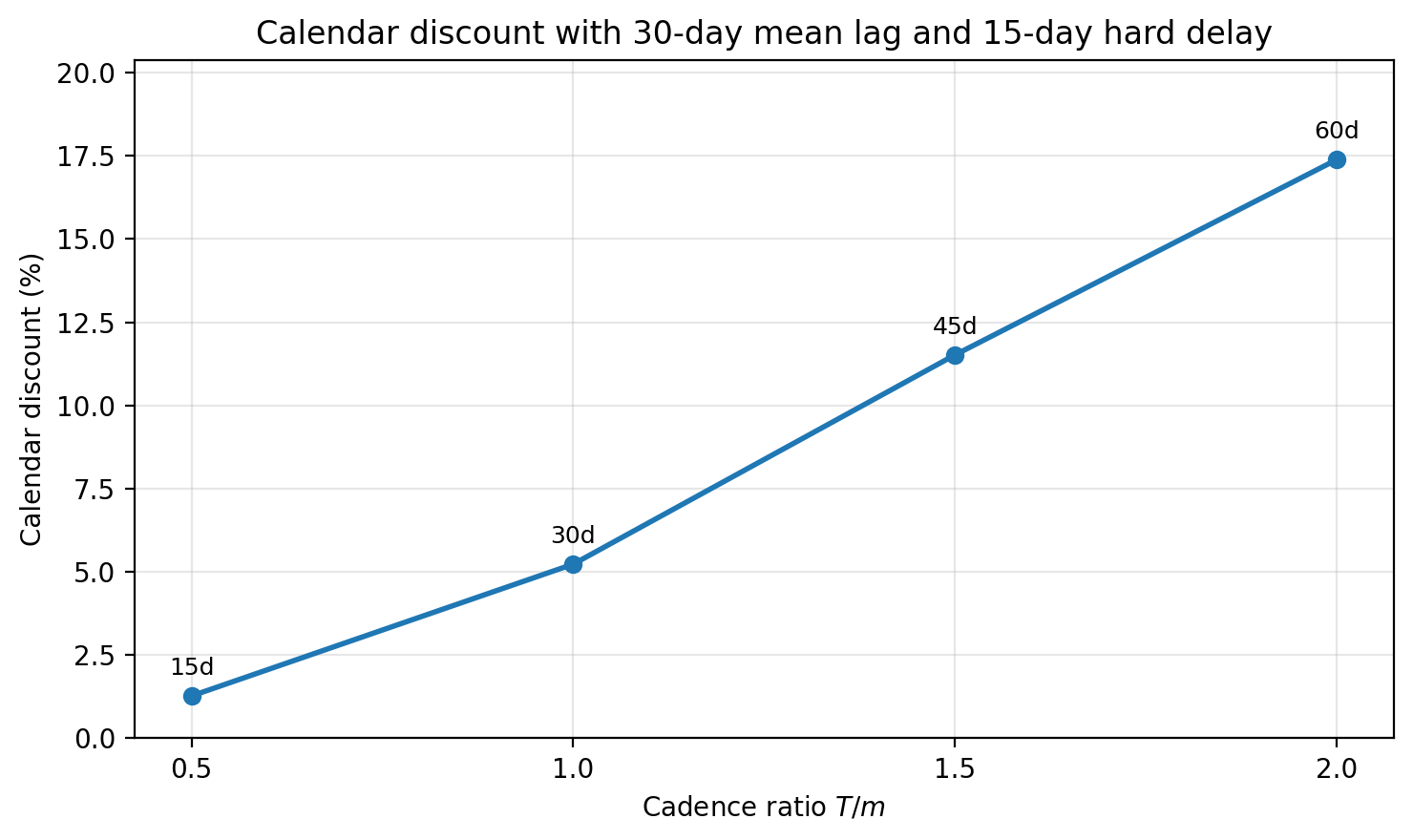
The headline worked packet uses the coarse two-month release train, \(T/m=2\) and \(\alpha=1\). This is a useful demonstration case because it keeps the reported mean lag at 30 days while making the fielding calendar material enough to be resolved with realistic evidence intervals. The packet is shown in Table 6. The same-mean shortcut classifies the local channel as inside capacity because the entire interval \(I_L=[2.657,2.756]\) lies below \(2.767\). The bimonthly calendar-aware calculation classifies the channel as outside capacity because the entire interval lies above \(2.286\). The calendar discount is \(17.4\%\). The result is therefore a resolved cadence warning: the mean remediation lag is not a safe fielding representation for this local claim.
| Field | Value | Audit interpretation |
|---|---|---|
| Routine mean lag | \(m=30\) days | Measured from routine remediation eligibility to effective fielded coverage, not only to ticket closure. |
| Routine release period | \(T=60\) days | Coarse two-month routine release train. |
| Release fraction | \(\alpha=1\) | All eligible routine backlog is fielded at each release window under the same-mean convention. |
| Non-fielding delay budget | \(\tau_\Sigma=15\) days | Detection, triage, validation, approval, testing, packaging, and other hard delays outside the release train. |
| Emergency channel | Excluded from routine mean | Emergency bypass has different timing rules and should be audited separately if included in the governance claim. |
| Residual-pressure interval | \(I_L=[2.657,2.756]\) | Computed from the notional local substitution ledger in Table [tbl:tab:worked-ledger]. |
| Continuous same-mean boundary | \(L_{\mathrm{crit}}^{\mathrm{cont}}\approx2.767\) | Mean-only capacity boundary under the normalized local-channel scenario. |
| Calendar-aware boundary | \(L_{\mathrm{crit}}^{\mathrm{cal}}\approx2.286\) | Capacity boundary under the bimonthly release calendar. |
| Calendar discount | \(\Delta_{\mathrm{cal}}\approx17.4\%\) | Fraction of mean-only capacity consumed by the recorded release calendar. |
| Audit status | Resolved cadence warning | The same packet is inside capacity under mean-only reporting but outside capacity under the bimonthly release calendar. |
The management reading is deliberately narrow:
For this local channel, evidence interval, hard-delay budget, and declared rate scenario, the reported 30-day mean lag is not sufficient fielding evidence. The release calendar consumes a material share of mean-only capacity and changes the local capacity verdict.
The same residual-pressure ledger can also be used to explain why the monthly case is different. At \(T/m=1\), the calendar-aware boundary is approximately \(2.623\) and the calendar discount is \(5.2\%\). The stated interval \(I_L=[2.657,2.756]\) still lies between the monthly and continuous capacity boundaries, so the point packet remains a resolved warning. However, the smaller discount means that the verdict is more sensitive to scoring resolution. This is the practical value of reporting \(\Delta_{\mathrm{cal}}\): a monthly cadence may be cadence-sensitive, but the organization needs a sharper residual-pressure ledger to defend a binary inside/outside claim than it would need for a coarser release train.
Table 7 makes this explicit. Small perturbations of the notional ledger leave the bimonthly calendar concern visible, but quickly turn the monthly binary verdict into an input-resolution question. This is not a failure of the audit. It is one of the intended audit outputs: if the evidence is too coarse relative to the calendar discount, the team should report an input-resolution or calendar-discount finding rather than force a sharp verdict.
| Residual-pressure treatment | Implied \(I_L\) | Bimonthly \(T/m=2\) | Monthly \(T/m=1\) |
|---|---|---|---|
| Stated score intervals | \([2.657,2.756]\) | Resolved cadence warning | Resolved cadence warning, but with smaller evidence margin. |
| One off-diagonal score \(\pm0.02\) | \([2.673,2.739]\) | Resolved cadence warning | Resolved cadence warning. |
| One off-diagonal score \(\pm0.05\) | \([2.624,2.789]\) | Calendar-discount finding; sharp verdict limited by upper tail | Input-resolution limited near the continuous boundary. |
| Both off-diagonal scores \(\pm0.05\) | \([2.544,2.873]\) | Calendar-discount finding; sharp verdict limited by evidence width | Input-resolution limited. |
| Broad local evidence interval | \([2.50,2.90]\) | Material calendar discount; improve \(I_L\) for a binary verdict | Input-resolution limited. |
The audit also supports a closed-loop engineering reading. Starting from the bimonthly packet, shortening the routine release train to a monthly cadence reduces the calendar discount from \(17.4\%\) to \(5.2\%\), but does not fully remove the warning for the stated evidence interval. Shortening further to a two-week cadence, \(T/m=0.5\), raises the calendar-aware boundary to approximately \(2.732\) and reduces the discount to \(1.3\%\). At that point the point estimate \(L\approx2.706\) is inside capacity under the calendar-aware calculation, but the interval \(I_L=[2.657,2.756]\) crosses the boundary. The right management conclusion is not that the intervention failed; it is that the cadence lever has largely removed the timing discount, and the remaining decision depends on residual-pressure evidence resolution or on reducing residual pressure through control improvement.
| Routine release calendar | Calendar discount | Status at \(I_L=[2.657,2.756]\) | Management reading |
|---|---|---|---|
| Two-month train, \(T/m=2\) | 17.4% | Resolved cadence warning | Mean-only reporting is unsafe for this local claim; cadence is a first-order governance variable. |
| Monthly train, \(T/m=1\) | 5.2% | Resolved but resolution-sensitive warning | Calendar still matters, but sharper local evidence is needed to defend a binary verdict under moderate perturbations. |
| Two-week train, \(T/m=0.5\) | 1.3% | Threshold-adjacent / input-resolution limited | Cadence discount is largely removed; remaining decision depends on improving \(I_L\) or reducing residual pressure. |
These worked packets establish three operational points before the model is introduced. First, two remediation processes can report the same 30-day mean lag while consuming very different fractions of mean-only local capacity. Second, the calendar discount is useful even when \(I_L\) is too coarse for a sharp inside/outside verdict. Third, the audit links a warning to an engineering test: shorten the release period, increase the release fraction, separate emergency and routine channels, reduce hard delay, compute cohort-phase effects, or improve the local BAS/control-validation ledger.
The next section gives the minimal calculation that produces the capacity boundaries used in these packets. The following section explains why release windows can change the verdict even when the mean lag is matched, and Section 6 checks the release-geometry conclusions under hard-delay placement, deployment rings, and cohort phasing.
4 From the audit packet to calendar discount↩︎
The worked packets in Section 3 used capacity boundaries and calendar discounts before introducing the calculation that produces them. This section defines that calculation as an audit interface. It is not a SOC simulator, a breach model, or a general theory of rollout kernels. It specifies what the backend consumes, what it returns, and how the returned quantities are used in a remediation-cadence audit. The local-channel state equations, release-cycle construction, and characteristic-equation details are kept in 10; the main text gives only the objects needed to reproduce and interpret the audit.
The backend consumes the audit packet defined in Section 2: the routine mean lag \(m\), release-window period \(T\), per-window release fraction \(\alpha\), cohort phases or ring geometry, emergency/routine channel split, non-fielding delay budget \(\tau_\Sigma\), residual-pressure interval \(I_L=[L_-,L_+]\), and the declared local-channel rate scenario. The rate scenario matters because the capacity boundaries are not universal constants. The worked packets use a normalized screening convention in which local defensive-revision and attacker-adjustment rates are measured in units of the routine mean lag. A production audit should either declare this screening convention, supply local rate estimates, or run a scenario band over plausible rates. If the calendar discount changes materially across that band, the correct audit output is a rate-scenario limitation rather than a sharp cadence verdict.
The backend compares two fielding representations of the same routine remediation process. The first is the continuous same-mean shortcut: the routine mean lag is treated as if defensive fielding catches up smoothly. This is the representation implicitly used when a dashboard mean is treated as the fielding process itself. The second is the calendar-aware release representation: routine changes wait for release windows, and at each window only the recorded fraction of the eligible backlog is fielded. Rings and cohort phases are handled as release geometry. Emergency bypass is excluded from the routine representation unless it is explicitly modeled as a separate channel.
For a synchronized routine release train, the same-mean comparison uses the idealized fielding mean \[m_{\mathrm{cal}} = \frac{T}{2} + T\frac{1-\alpha}{\alpha}. \label{eq:calendar-mean-lag}\tag{3}\] This formula has a simple operational reading. The first term is the average waiting time until the next release window under uniformly distributed arrival phase. The second term is the additional expected waiting created when each window clears only a fraction \(\alpha\) of the remaining eligible backlog. In the worked packets, \(m_{\mathrm{cal}}\) is matched to the reported routine mean lag so that the comparison isolates release geometry rather than average remediation speed. In a production audit, \(m\), \(T\), and \(\alpha\) should come from deployment telemetry. If the mean implied by coverage telemetry does not match the reported MTTR, that mismatch is itself an audit finding.
The calculation returns four quantities, summarized in Table 9. The first is the mean-only capacity boundary, \(L_{\mathrm{crit}}^{\mathrm{cont}}\). The second is the calendar-aware capacity boundary, \(L_{\mathrm{crit}}^{\mathrm{cal}}\), for the recorded release geometry. The third is the calendar discount, already introduced in Section 2. The fourth is the position of the residual-pressure interval \(I_L\) relative to the two boundaries.
| Backend object | What it means | How the audit uses it |
|---|---|---|
| \(L_{\mathrm{crit}}^{\mathrm{cont}}\) | Mean-only capacity boundary under the continuous same-mean shortcut. | Benchmark for the claim implicitly made when MTTR is treated as a fielding model. |
| \(L_{\mathrm{crit}}^{\mathrm{cal}}\) | Calendar-aware capacity boundary under the recorded release process. | Tests whether release windows, release fraction, rings, hard delay, or channel splitting change the local capacity verdict. |
| \(\Delta_{\mathrm{cal}}\) | Fraction of mean-only local capacity consumed by calendarized fielding. | Reports how much evidence resolution is needed before a mean-only fielding claim is defensible. |
| Position of \(I_L\) | Residual-pressure interval relative to both boundaries. | Determines whether the finding is mean-only adequate, resolved cadence warning, calendar-discount finding, outside under both, input-resolution limited, or scenario-limited. |
The most important audit case is no longer only a point estimate between two thresholds. A resolved cadence warning occurs when the residual-pressure interval is below the mean-only boundary but above the calendar-aware boundary: \[L_{\mathrm{crit}}^{\mathrm{cal}} < L_- \le L_+ < L_{\mathrm{crit}}^{\mathrm{cont}} .\] In that case the same remediation packet is inside capacity under mean-only reporting but outside capacity under the actual release calendar. A calendar-discount finding is weaker but still useful: \(I_L\) may be too wide for a binary verdict, yet the discount may be material relative to the claimed headroom. This is the situation in which the audit tells the team that MTTR/SLA should not be used alone unless release-calendar evidence is disclosed and tested.
The calculation can also return an input-resolution or scenario limitation. If the uncertainty in \(I_L\), \(\alpha\), \(T\), cohort phases, or \(\tau_\Sigma\) is wider than the calendar effect being tested, the audit should not force a sharp inside/outside verdict. If the result changes across plausible local-channel rate scenarios, the audit should report a scenario band rather than a single threshold. These outcomes are not failures of the method. They are governance findings: the organization lacks enough evidence resolution to defend a mean-only fielding claim for the local channel.
The same interface also explains how to read engineering interventions. Changing the release period \(T\), the release fraction \(\alpha\), the hard-delay budget \(\tau_\Sigma\), cohort phases, or the emergency/routine channel split changes \(L_{\mathrm{crit}}^{\mathrm{cal}}\) and therefore \(\Delta_{\mathrm{cal}}\). Reducing residual attacker pressure through better controls, detection, or response changes \(I_L\). The audit is useful because it keeps these two levers separate: one lever changes the fielding process, the other changes the local residual-pressure evidence.
This interface is the only calculation layer needed in the main text. The next section explains why release windows can reduce the calendar-aware capacity boundary even when the mean lag is matched. 10 records the local-channel equations used by the backend, 11 gives the small-cadence result, 12 shows why same-mean fielding processes need not be equivalent, and 13 summarizes the independent numerical check used in Section 6.
5 Why release windows create a calendar discount↩︎
Section 4 defined the calculation interface: the audit packet is converted into a mean-only capacity boundary, a calendar-aware capacity boundary, a calendar discount, and an evidence-resolution status. This section explains why the calendar-aware boundary can be lower even when the reported mean remediation lag is held fixed. The detailed perturbation calculation is given in 11; the main text keeps only the operational mechanism and the quantities needed for the audit.
The mechanism is simple. A continuous same-mean shortcut lets the fielded defensive posture catch up at every instant. A release calendar does not. It holds routine changes until the next window, then fields the recorded fraction of the eligible backlog. During the waiting part of the cycle, the estate continues to operate with stale fielded posture. During the release part of the cycle, the correction arrives in synchronized batches. Matching the average lag does not match this timing response. Two remediation processes can therefore have the same reported mean lag while exposing the local channel to different fielding dynamics.
For the normalized local-channel backend, synchronized release windows reduce the calendar-aware capacity boundary initially by a second-order cadence effect: \[L_{\mathrm{crit}}^{\mathrm{cal}}(T) = L_{\mathrm{crit}}^{\mathrm{cont}} - \mathfrak c T^2 + O(T^4), \qquad \mathfrak c>0 . \label{eq:s5-small-cadence}\tag{4}\] This expression is not used to compute the finite worked-packet values. It is a local explanation of direction: when routine fielding is synchronized into windows, the calendar-aware capacity boundary moves downward from the continuous same-mean boundary. The finite monthly, six-week, and bimonthly values used in the audit are computed directly from the release-window backend.
The audit reports this loss as the calendar discount: \[\Delta_{\mathrm{cal}} = \frac{ L_{\mathrm{crit}}^{\mathrm{cont}} - L_{\mathrm{crit}}^{\mathrm{cal}} }{ L_{\mathrm{crit}}^{\mathrm{cont}} } . \label{eq:s5-calendar-discount}\tag{5}\] The discount is not a breach probability and not a vulnerability score. It is a fielding-governance quantity: the fraction of mean-only local capacity consumed by the recorded release calendar. This is the quantity that lets the audit stay useful when the residual-pressure interval is too coarse for a sharp binary verdict.
To interpret the discount, the audit also records the width of the residual-pressure interval relative to the mean-only boundary: \[W_L = \frac{L_+-L_-}{L_{\mathrm{crit}}^{\mathrm{cont}}}. \label{eq:s5-evidence-width}\tag{6}\] When \(W_L\) is small relative to \(\Delta_{\mathrm{cal}}\), the evidence is sharp enough to support a resolved inside/outside comparison. When \(W_L\) is comparable to or larger than \(\Delta_{\mathrm{cal}}\), the audit should usually report an input-resolution or calendar-discount finding rather than force a binary verdict. This is not a failure of the method. It is the method telling the organization that its residual-pressure evidence is too coarse to justify using MTTR as a fielding model.
Table 10 gives the practical reading used in this paper. The bands are not universal policy thresholds; they are an audit language for relating timing loss to evidence resolution. A small discount may still matter for a high-assurance channel with sharp BAS/control-validation evidence. A larger discount should be treated as a first-order governance variable even when residual-pressure evidence is coarse.
| Calendar discount | Evidence-resolution reading | Typical governance action |
|---|---|---|
| Below about \(3\%\) | Usually smaller than ordinary scoring and telemetry uncertainty, unless the local ledger is unusually sharp. | Report cadence as recorded; improve evidence if a sharp capacity verdict is required. |
| About \(3\)–\(8\%\) | Potentially material but resolution-sensitive. A binary verdict requires a well-supported residual-pressure interval. | Disclose the release calendar and test whether BAS/control-validation evidence can resolve the discount. |
| About \(8\)–\(15\%\) | Often large enough to be visible with practical evidence intervals. | Treat cadence as a governance variable; test shorter windows, larger release fractions, or hard-delay reduction. |
| Above about \(15\%\) | Calendarized fielding consumes a large share of mean-only capacity. | Do not use MTTR/SLA alone as fielding evidence; run a calendar-aware audit before making the local capacity claim. |
For the normalized delayed scenario used in the worked packets, \(\tau_\Sigma/m=0.5\) and \(L_{\mathrm{crit}}^{\mathrm{cont}}\approx2.767\). Holding the reported mean lag fixed at 30 days, a two-week release screen has a discount of about \(1.3\%\), a monthly release train about \(5.2\%\), a six-week train about \(11.5\%\), and a bimonthly train about \(17.4\%\). These values explain why the bimonthly packet in Section 3 is a cleaner headline demonstration than the monthly packet. The monthly case is operationally common and still important, but its discount is narrow enough that a sharp binary verdict requires unusually good residual-pressure evidence. The bimonthly case has the same reported mean lag but a much larger discount, so the calendar effect remains visible with coarser evidence intervals.
The same logic explains the closed-loop intervention reading. If a bimonthly routine release train is shortened to monthly, the discount falls substantially but may remain resolution-sensitive. If it is shortened further, the calendar discount may become small relative to the residual-pressure uncertainty; at that point the cadence lever has largely removed the timing loss, and the remaining decision depends on improving the local ledger or reducing residual pressure through control changes. The audit therefore separates two engineering levers: change the fielding process to move \(L_{\mathrm{crit}}^{\mathrm{cal}}\), or change the security posture to move \(I_L\).
Hard delay does not remove this interpretation. Detection, validation, approval, packaging, and testing delays reduce the available local capacity in both the same-mean and calendar-aware representations. The release calendar then determines how much additional capacity is consumed by batching routine fielding into windows. Section 6 checks that the calendar gap is not an artifact of assigning the same hard-delay budget to one side of the feedback loop.
The discount also depends on the declared local-channel rate scenario. The worked packets use the normalized screening convention, but production audits should either declare that convention or run a scenario band over plausible local rates. If the discount remains in the same practical band across the scenario range, the cadence finding is robust. If the discount moves from, for example, a negligible band to a material band when the rate scenario changes, the correct output is a rate-scenario limitation. This is why the rate scenario is part of the audit packet rather than a hidden modeling choice.
Finally, calendar discount is not eliminated by saying that a release train uses rings. Rings and cohort phases change the calendar-aware release geometry, and therefore can change \(L_{\mathrm{crit}}^{\mathrm{cal}}\) and \(\Delta_{\mathrm{cal}}\). They do not automatically recover the continuous same-mean shortcut. The next section validates this point numerically: adding equal-phase cohorts at fixed per-asset cadence approaches a phase-averaged calendar process, not the continuous benchmark, and cohort staggering can help or hurt near capacity.
The practical result of this section is the audit rule used throughout the rest of the paper:
Do not ask only whether a point estimate of \(L\) lies between two thresholds. Report the calendar discount and compare it with the residual-pressure evidence resolution. If the discount is material relative to the claimed headroom or the evidence width, MTTR/SLA should not be used alone as a fielding representation.
11 gives the small-cadence derivation. 12 shows independently why same-mean fielding processes need not be equivalent. Section 6 then checks the finite running values, hard-delay placement, and cohort-geometry effects used by the audit.
6 Validation and release-geometry checks↩︎
The worked packets and the calendar-discount interpretation rely on finite release-window boundaries, not on the small-cadence approximation alone. This section checks that the practical findings are not artifacts of one numerical implementation, one hard-delay placement, or one rate scenario. The checks are reported as security-operations validation rather than as a numerical-methods section. The technical backend uses an exact one-cycle release map for the single-total-delay case and collocation cross-checks for alternative delay placements; implementation details are summarized in Appendix 13.
The validation addresses five questions. First, do the finite calendar-aware boundaries used in the audit stabilize under the independent backend? Second, is the calendar-discount reading robust over a plausible attacker-adjustment rate band? Third, does the calendar discount survive alternative placements of the same hard-delay budget? Fourth, does splitting a release train into more cohorts recover the continuous same-mean benchmark? Fifth, is cohort staggering always beneficial? The answers are: yes, qualitatively yes for the practical bands used here, yes, no, and no. These are the release-geometry facts a security team needs before relying on MTTR/SLA as fielding evidence.
The monthly point is the most resolution-sensitive worked case because its calendar discount is only about \(5.2\%\) under the normalized screening scenario. It is therefore a useful numerical stress test: if the backend is unstable, this narrow case would be the first to move. For the normalized delayed scenario, \[T/m=1,\qquad \alpha=2/3,\qquad \tau_\Sigma/m=0.5,\] the continuous same-mean boundary is \[L_{\mathrm{crit}}^{\mathrm{cont}}=2.767423\ldots .\] Table 11 reports the independent calendar-aware boundary as the backend resolution is increased. The boundary stabilizes at approximately \(2.623\). Thus the monthly discount used in the worked packet, \[\Delta_{\mathrm{cal}} = \frac{2.767423-2.622676}{2.767423} \approx 5.2\% ,\] is not a visible artifact of the backend resolution.
| Backend resolution | \(L_{\mathrm{crit}}^{\mathrm{cal}}\) |
|---|---|
| 4 | 2.622481 |
| 6 | 2.622681 |
| 8 | 2.622678 |
| 10 | 2.622677 |
| 12 | 2.622676 |

The second check concerns the rate scenario. The worked packets use the normalized screening convention \(\kappa=1\), but the audit record requires the rate scenario to be declared rather than hidden. Table 12 therefore reports the calendar-discount band over a 16-fold range of attacker-adjustment rates, \(\kappa\in[0.25,4]\), with the same normalized hard-delay budget \(\tau_\Sigma/m=0.5\). The qualitative reading is stable. The two-week screen remains below \(2\%\), the monthly train stays in the resolution-sensitive \(3\)–\(8\%\) band, and the two-month train remains material throughout the band, never falling below about \(12\%\). The bimonthly discount is not monotone in \(\kappa\), so production audits should report a scenario band rather than a single point when local rates are uncertain.
| \(\kappa\) | \(T/m=0.5\) | \(T/m=1.0\) | \(T/m=1.5\) | \(T/m=2.0\) | \(L_{\mathrm{crit}}^{\mathrm{cont}}\) |
|---|---|---|---|---|---|
| 0.25 | 0.86% | 3.44% | 7.79% | 13.39% | 4.2795 |
| 0.50 | 1.04% | 4.20% | 9.44% | 15.65% | 3.1497 |
| 1.00 | 1.27% | 5.23% | 11.52% | 17.38% | 2.7674 |
| 2.00 | 1.53% | 6.52% | 13.33% | 16.35% | 2.7972 |
| 4.00 | 1.75% | 7.88% | 13.61% | 12.42% | 2.9994 |
The third check concerns the non-fielding delay budget. In the worked packets, \(\tau_\Sigma/m=0.5\) represents detection, triage, validation, approval, testing, packaging, and other delays outside the routine release train. A reviewer may ask whether the calendar gap is created by placing that hard delay on one side of the local channel. The independent verification answers this more strongly than a split table: for the monthly packet, placing the same total delay on the fielded-posture-to-attacker link, sampling the intended posture at \(t_n-\tau_\Sigma\), or placing the delay on either feedback direction gives the same calendar-aware boundary to less than \(10^{-5}\). In all cases the monthly boundary is \(2.622676\ldots\). The calendar discount is therefore a release- calendar effect, not a bookkeeping artifact of where the same total hard-delay budget is placed.
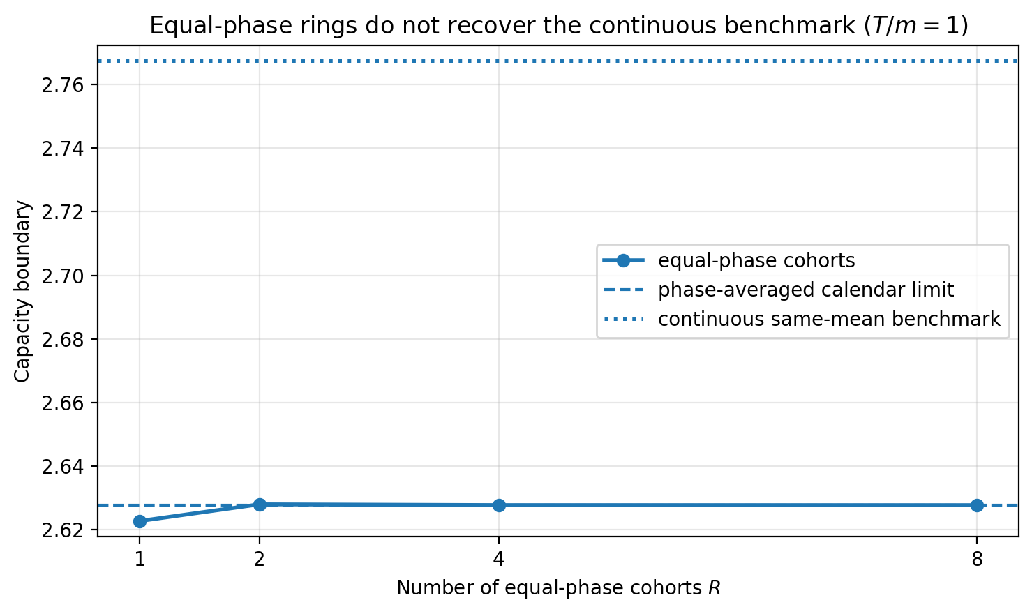
The fourth check concerns deployment rings. A common operational response to a cadence warning is to say that the release train is not synchronized because it uses rings. Rings can be useful, but they do not automatically justify the continuous same-mean shortcut. At fixed per-asset cadence, increasing the number of equal-phase cohorts converges to a phase-averaged calendar process, not to continuous fielding. Each asset still sees a release calendar.
Table 13 shows the effect for the monthly case. Equal-phase cohorts move the calendar-aware boundary slightly upward, from about \(2.623\) to about \(2.628\). That is a real improvement, but it does not recover the continuous same-mean boundary \(2.767423\ldots\). The calendar discount remains about \(5\%\). The operational conclusion is direct: a team cannot defend mean-only reporting merely by saying that monthly release is split into rings. The ring geometry must be recorded and checked.
| Release geometry | Calendar-aware boundary | Calendar discount |
|---|---|---|
| Synchronized monthly release, \(R=1\) | 2.623 | 5.2% |
| Equal-phase cohorts, \(R=2\) | 2.628 | 5.0% |
| Equal-phase cohorts, \(R=4\) | 2.628 | 5.0% |
| Equal-phase cohorts, \(R=8\) | 2.628 | 5.0% |
| Dense equal-phase calendar limit | 2.628 | 5.0% |
| Continuous same-mean shortcut | 2.767 | 0.0% |
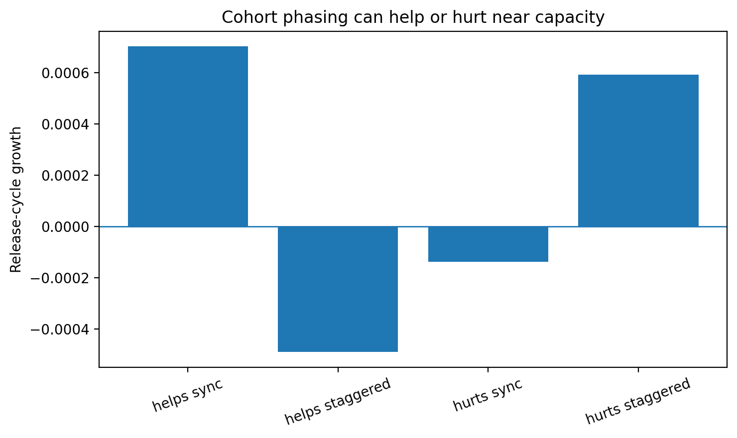
The fifth check is whether staggering is always stabilizing. It is not. Cohort phasing is a release-geometry variable, not a universal remedy. Near a capacity boundary, different phase schedules can move the local channel in different directions. Table 14 gives two near-boundary examples. In the first, equal staggering turns a small positive growth rate into a small negative one. In the second, equal staggering turns a small negative growth rate into a positive one. The point is not that staging is bad. The point is that the phase schedule must be treated as evidence, not as a verbal substitute for the continuous shortcut.
| Case | \(T/m\) | \(L\) | Synchronized growth | Equal-staggered growth, \(R=4\) |
|---|---|---|---|---|
| Staggering helps | 1.5 | 2.456 | 0.000703 | -0.000490 |
| Staggering hurts | 1.8 | 2.342 | -0.000138 | 0.000593 |
Together, the checks support the audit interpretation without overclaiming. The finite monthly boundary is numerically stable; the discount bands are stable in practical terms across a broad \(\kappa\) scenario range; the calendar boundary is invariant to tested placements of the same total hard-delay budget; deployment rings at fixed per-asset cadence do not recover the continuous same-mean benchmark; and cohort staggering can help or hurt near capacity. These are fielding-governance findings. They tell a security team when release-calendar evidence must be recorded and tested before MTTR/SLA is used as a fielding model.
7 Related work and positioning↩︎
This paper sits at the intersection of enterprise vulnerability management, security measurement, remediation governance, adversary emulation, and timing models. Its contribution is not a new vulnerability-severity score, a new exploit-prediction model, or a general adaptive-defense theory. The contribution is narrower: a remediation-cadence audit that tests whether a mean remediation metric is a safe fielding representation, and that reports the calendar discount and evidence-resolution status when release geometry is hidden by MTTR/SLA reporting.
Enterprise patch-management guidance provides the operational setting. NIST frames enterprise patch management as a preventive-maintenance process involving identification, prioritization, acquisition, installation, and verification of patches [1]. Public vendor and cloud documentation shows that routine security updates, scheduled maintenance windows, recurring patching configurations, and out-of-band update paths are ordinary operational objects rather than theoretical constructs [2], [3]. These sources motivate the timing fields in the audit packet: release-window period, release fraction, maintenance window, emergency bypass, and effective fielded coverage.
Security-metrics work motivates the caution against mean-only reporting. Quantified security metrics are useful for governance, but prior surveys and critical reviews emphasize that aggregate measures can be weakly validated, context-dependent, and difficult to interpret operationally [11], [12]. Vulnerability-management studies and industry remediation analyses also show that remediation data can be skewed, long-tailed, censored, or sensitive to the definition of closure [6]. The present audit follows this measurement tradition but focuses on one hidden variable: release cadence. The issue is not only whether the mean remediation lag is high or low; it is whether the mean is a defensible fielding model for the local security claim being made.
Vulnerability scoring, exploitability signals, and known-exploited-vulnerability programs are adjacent but not substitutes for the residual-pressure input used here. CVSS provides a standardized severity framework [7]; EPSS and related work estimate exploitation likelihood or help prioritize remediation [8], [13]; empirical studies compare vulnerability severity with observed exploitation [14], [15]; and remediation-selection work addresses how to choose which vulnerabilities to fix under constraints [16]. CISA’s KEV catalog and risk-based remediation directives illustrate governance based on known exploitation and remediation deadlines [4], [5]. These signals are important for scope and prioritization, but they do not describe how fixes are fielded through release windows, rings, change freezes, or emergency bypass paths. They also do not provide a local residual-pressure interval after an organization’s specific controls, detections, response processes, and compensating measures are taken into account.
The residual-pressure ledger is instead connected to adversary-emulation and control-validation practice. MITRE ATT&CK provides a shared vocabulary for techniques and defensive observations [9]. CALDERA and Atomic Red Team illustrate repeatable adversary-emulation and ATT&CK-mapped testing practices [17], [18]. NIST SP 800-53A provides a general assessment frame for evaluating whether controls are implemented and effective [19]. The audit does not depend on any one tool or framework. It requires the local ledger to identify the technique family, defender posture, score interval, evidence source, observation window, and reviewer. This is why \(L\) is treated as a local evidence interval rather than as a public CVE-derived score.
The work also relates to moving-target defense, deception, timing games, and adaptive security models. FlipIt-style games and moving-target defense surveys study the timing of attack and defense, reconfiguration, and strategic adaptation [20]–[23]. Work on patching dynamics and epidemic-style remediation models studies how updates or security actions propagate through populations [24], [25]. These literatures establish that timing and adaptation matter. The present paper addresses a more specific enterprise-operations question: when a team reports remediation through a mean lag, does the release calendar consume enough local capacity that the mean should not be used as the fielding model?
Finally, sampled-data, networked-control, and delay-system methods provide the technical backend used to compute the capacity boundaries and release-geometry checks [26]–[32]. This backend explains why same-mean fielding processes need not be equivalent and why synchronized release windows can create a calendar discount. However, the article’s security contribution is not the backend itself. The contribution is the audit interface: an operational packet, a same-mean versus calendar-aware comparison, a calendar discount, an evidence-resolution reading, and a governance status that tells enterprise teams when release-calendar evidence must be disclosed and tested before MTTR/SLA is used as fielding evidence.
8 Limitations and responsible use↩︎
The audit is intentionally limited. It is a local fielding diagnostic, not a breach prediction, exploit-probability model, CVE prioritizer, or complete enterprise risk model. A calendar-discount finding means that the release calendar consumes a material part of mean-only local capacity, or that the available evidence is too coarse to justify treating MTTR as a fielding model. It does not mean that an incident will occur, that a specific vulnerability should be patched first, or that calendarized release trains are generally unsafe.
The worked packets are not empirical calibrations on a named enterprise dataset. The timing side is motivated by public operational artifacts such as release cycles, scheduled patching, maintenance windows, out-of-band update paths, KEV governance, and remediation-measurement studies. The residual-pressure ledger, however, is notional. This is appropriate for a method paper, but it limits the claim: the paper demonstrates how the audit is run, how a calendar discount is reported, and how evidence resolution changes the interpretation. It does not estimate how frequently such findings occur across enterprises.
The residual-pressure interval \(I_L\) is the most important local input and the largest source of governance risk. It depends on score construction, evidence quality, defender-posture taxonomy, technique grouping, and the mapping from BAS, red-team, purple-team, control-validation, postmortem, or expert-scored evidence to the audited local channel. The two-by-two ledger used in the worked packets is a minimal substitution ledger, not a universal enterprise risk matrix. Production use should report the scoring rubric, evidence sources, observation window, reviewer, sign-off authority, and an interval rather than an unsupported point value.
The calendar discount also depends on the declared local-channel rate scenario. The worked packets use a normalized screening convention. This convention is useful for demonstrating the audit and for comparing release geometries, but it is not a calibrated enterprise forecast. A production audit should either declare the normalized convention, supply local rate estimates, or run scenario bands over plausible defensive-revision and attacker-adjustment rates. If the discount or status changes materially across the scenario band, the appropriate output is a rate-scenario limitation rather than a single sharp verdict.
The remediation timing inputs can also be imperfect. MTTR may be censored, right-tailed, asset-dependent, or based on ticket closure rather than effective fielded coverage. Release fraction \(\alpha\) may differ across platforms, asset classes, and maintenance windows. Cohort phases and ring policies may differ between policy documents and actual deployment telemetry. Emergency and routine remediation paths may be mixed in one dashboard mean even though they follow different timing, approval, testing, and coverage rules. The audit is only as reliable as the deployment-coverage and delay-budget evidence used to populate the packet.
The model itself is local and deliberately simplified. The main calculation treats one local adaptation channel and a declared routine cadence. It does not model strategic attacker anticipation of release calendars, adversarial manipulation of emergency-bypass rules, correlated enterprise-wide failures, multi-channel coupling, asset-dependent exploit chains, or mode-dependent cadence in which different attacker techniques and defender postures have different fielding laws. These are important extensions, but including them in the main audit would make the procedure less usable for security operations.
Responsible use therefore requires conservative interpretation. A resolved cadence warning should trigger engineering tests of release period, release fraction, hard-delay budget, cohort phases, emergency/routine channel separation, and residual-pressure reduction. A calendar-discount finding should trigger disclosure and testing of the release calendar before MTTR/SLA is used as fielding evidence. An input-resolution finding should trigger better BAS, control-validation, deployment-coverage, or delay-budget evidence. These statuses are not failures of the audit. They are the audit’s intended governance outputs.
9 Conclusion↩︎
MTTR and SLA compliance are useful remediation metrics, but they are not fielding models. They summarize how long remediation takes on average; they do not describe how fixes actually reach the estate through release windows, maintenance periods, rings, partial backlog clearing, hard delays, and emergency bypass paths. This paper introduced a remediation-cadence audit for that gap. The audit records the routine mean lag, release period, release fraction, cohort geometry, emergency/routine channel split, non-fielding delay budget, residual-pressure interval, and local-channel rate scenario, then compares a continuous same-mean shortcut with the recorded release calendar.
The main output is the calendar discount: the fraction of mean-only local capacity consumed by calendarized routine fielding. This shifts the audit away from a fragile point comparison and toward an evidence-resolution question. If the discount is small relative to the residual-pressure evidence width, the right finding may be input-resolution limited. If the discount is material relative to the claimed headroom, MTTR/SLA should not be used alone as fielding evidence. If the residual-pressure interval is resolved across the two capacity boundaries, the audit returns a cadence warning.
The worked packets show how this reading changes the operational message. With the same reported 30-day mean lag and the same non-fielding delay budget, a coarse two-month release train consumes about 17.4% of mean-only local capacity, while a monthly train consumes about 5% and a shorter two-week screen about 1%. The coarser case is easier to resolve with practical residual-pressure evidence; the monthly case is more resolution-sensitive. This distinction is the point of the audit. It tells a security team not only whether a point estimate falls between two boundaries, but also how much evidence resolution is needed before a mean-only fielding claim is defensible.
The release-geometry checks add two practical findings. Splitting a monthly release train into equal-phase deployment rings at fixed per-asset cadence does not recover the continuous same-mean benchmark; it approaches a phase-averaged calendar process. Cohort staggering is also not automatically stabilizing near capacity. It can help or hurt depending on the local channel and phase schedule. Rings and cohort phases therefore belong in the audit packet rather than in a verbal assurance that rollout is “staged.”
The practical implication is simple. A vulnerability-management program should not treat MTTR/SLA as complete fielding evidence when the release calendar can consume a material share of local capacity. The team should record cadence, release fraction, rings, emergency bypass, hard delay, residual-pressure evidence, and rate scenario; compute the calendar discount; compare it with evidence resolution; and choose the next engineering test. The audit does not replace vulnerability prioritization or incident response. It gives enterprise security teams a reproducible way to decide when the remediation calendar itself must be disclosed and tested before a mean remediation metric is used in security-governance claims.
Data and code availability↩︎
The worked packets use a notional residual-pressure ledger and do not contain enterprise-confidential data. A supplementary reproducibility package is provided with the manuscript. It includes an audit-packet template, a residual-pressure ledger template, the notional worked packet, the notional ledger, source data for the figures and tables, a verdict-classification script, and an exact running-case backend script that recomputes the continuous boundary, finite calendar-aware boundaries, calendar discounts, and the \(\kappa\) scenario band reported in the paper.
The supplementary scripts reproduce the audit reading and the reported running-case checks; they do not infer residual pressure from public CVE, CVSS, EPSS, KEV, OSV, or advisory data. Public sources are used only to anchor timing and governance context. Production use must replace the notional ledger with local BAS, red-team, control-validation, postmortem, or expert-scored evidence and should report uncertainty intervals and rate-scenario assumptions.
10 Local-channel backend equations↩︎
This appendix records the local-channel backend used by the audit calculation. The main text treats the calculation as an interface from an audit packet to capacity boundaries and calendar discount. This appendix gives the state representation used to compute those quantities.
All timing quantities can be nondimensionalized by the routine mean lag \(m\). The worked packets use the normalized screening convention \[m=1,\qquad \mu_X=\mu_Y=\kappa=1,\] with the non-fielding delay reported as \(\tau_\Sigma/m\). A production audit may instead supply local rate estimates or run a scenario band over plausible rate ratios. The rate scenario is therefore part of the audit packet rather than a hidden modeling choice.
Let \(a(t)\) denote the intended defensive revision and \(x(t)\) the defensive posture actually fielded on the estate. Let \(b(t)\) denote the attacker’s intended technique adjustment and \(y(t)\) the technique share actually in use. Before inserting the separate non-fielding delay budget, the local-channel backend is \[\begin{align} \dot{a}(t)&=-\mu_X a(t)+\sqrt L\,y(t),\\ \dot{b}(t)&=-\mu_Y b(t)-\sqrt L\,x(t),\\ \dot{y}(t)&=\kappa\bigl(b(t)-y(t)\bigr). \end{align} \label{eq:app-local-channel-flow}\tag{7}\] The fielding rule for \(x(t)\) is the component changed by the audit comparison.
The continuous same-mean shortcut treats fielding as a smooth catch-up process, \[\dot{x}(t)=\frac{1}{m}\bigl(a(t)-x(t)\bigr). \label{eq:app-continuous-fielding}\tag{8}\] For this representation, without non-fielding delay, the local capacity boundary is obtained from \[D(z)+\kappa L=0, \qquad D(z)=(z+\mu_X)(z+\mu_Y)(z+\kappa)(1+mz). \label{eq:app-cont-characteristic}\tag{9}\] With a total non-fielding delay budget \(\tau_\Sigma\), the corresponding single-total-delay characteristic equation is \[e^{z\tau_\Sigma} (z+\mu_X)(z+\mu_Y)(z+\kappa)(1+mz) +\kappa L=0. \label{eq:app-cont-characteristic-delay}\tag{10}\] The continuous same-mean boundary \(L_{\mathrm{crit}}^{\mathrm{cont}}\) is the value of \(L\) at which the principal root has zero real part.
The synchronized release-window representation holds routine fielding between release windows and updates the fielded posture at release times \(t_n=nT\): \[\dot{x}(t)=0,\qquad t\ne t_n, \label{eq:app-between-releases}\tag{11}\] \[x(t_n^+)=(1-\alpha)x(t_n^-)+\alpha a(t_n^-). \label{eq:app-calendar-release-rule}\tag{12}\] Rings and cohort phases apply the same release rule to cohorts at their recorded phases. Emergency bypass is not included in this routine rule unless the emergency path is explicitly modeled as a separate channel.
For the no-delay synchronized case, write \(s=(a,b,x,y)^\top\). Between release windows, \[\dot{s}(t)=A_Ls(t), \qquad A_L= \begin{pmatrix} -\mu_X&0&0&\sqrt L\\ 0&-\mu_Y&-\sqrt L&0\\ 0&0&0&0\\ 0&\kappa&0&-\kappa \end{pmatrix}, \label{eq:app-AL}\tag{13}\] and the release update is \[J_\alpha= \begin{pmatrix} 1&0&0&0\\ 0&1&0&0\\ \alpha&0&1-\alpha&0\\ 0&0&0&1 \end{pmatrix}. \label{eq:app-Jalpha}\tag{14}\] The one-window release-cycle matrix is \[M_L(T)=J_\alpha e^{A_LT}. \label{eq:app-release-cycle-matrix}\tag{15}\] The no-delay calendar-aware capacity boundary is obtained from \[\rho\!\left(M_L(T)\right)=1, \label{eq:app-rho-boundary}\tag{16}\] where \(\rho(\cdot)\) is spectral radius. Equivalently, the release-cycle growth rate is \[g_{\mathrm{cal}}(T,L)=\frac{1}{T}\log \rho\!\left(M_L(T)\right), \label{eq:app-growth-rate-no-delay}\tag{17}\] and the boundary satisfies \(g_{\mathrm{cal}}(T,L_{\mathrm{crit}}^{\mathrm{cal}})=0\).
With positive non-fielding delay, the same idea is implemented by the independent delay-equation backend summarized in 13. The finite monthly, six-week, and bimonthly thresholds reported in the main text are computed from the release-window backend, not from the small-cadence asymptotic formula.
For an idealized synchronized release process with uniformly distributed arrival phase and geometric clearing of the remaining eligible backlog, the mean fielding lag is \[m_{\mathrm{cal}}=\frac{T}{2}+T\frac{1-\alpha}{\alpha}. \label{eq:app-calendar-mean}\tag{18}\] This is the same-mean convention used in the worked packets. Production audits should estimate \(m\), \(T\), and \(\alpha\) from deployment telemetry and treat any mismatch between reported MTTR and empirical coverage timing as an audit finding.
11 Small-cadence release-window penalty↩︎
This appendix gives the perturbation result behind the calendar-discount interpretation. The main text uses only the operational consequence: synchronized release windows can lower the calendar-aware capacity boundary even when the mean fielding lag is matched. The finite thresholds used in the worked packets are computed directly; the result below explains the direction of the effect for small release periods.
Let \(N\) be the fielding-update direction \[N= \begin{pmatrix} 0&0&0&0\\ 0&0&0&0\\ 1&0&-1&0\\ 0&0&0&0 \end{pmatrix}, \qquad N^2=-N. \label{eq:app-N}\tag{19}\] The release update can be written as \[J_\alpha=I+\alpha N=\exp(\beta N), \qquad \beta=-\log(1-\alpha).\] The continuous same-mean generator is \[G_0=A_L+\frac{1}{m}N,\] which corresponds to the smooth fielding law \(\dot{x}=(a-x)/m\).
Assume that the continuous same-mean backend has a simple principal critical point \[z_0=i\omega_0,\qquad \omega_0>0,\] at branch strength \(L_0\), so that \[D(i\omega_0)+\kappa L_0=0, \qquad D'(i\omega_0)\ne0, \label{eq:app-principal-crossing}\tag{20}\] where \[D(z)=(z+\mu_X)(z+\mu_Y)(z+\kappa)(1+mz).\] Define \[\Psi=\frac{D'(z_0)}{D(z_0)}. \label{eq:app-Psi}\tag{21}\] For the synchronized release rule with mean matching \[m=\frac{T}{2}+T\frac{1-\alpha}{\alpha}, \qquad \alpha(T)=\frac{T}{m+T/2}, \label{eq:app-mean-matching}\tag{22}\] the local calendar-aware capacity boundary has the expansion \[L_{\mathrm{crit}}^{\mathrm{cal}}(T) = L_0-\mathfrak cT^2+O(T^4), \qquad T\to0, \label{eq:app-main-expansion}\tag{23}\] where \[\mathfrak c = L_0\left( \operatorname{Re}q+ \operatorname{Im}q\, \frac{\operatorname{Im}\Psi}{\operatorname{Re}\Psi} \right), \qquad q=\frac{\omega_0^2}{12(1+im\omega_0)}. \label{eq:app-c-coefficient}\tag{24}\] For the principal simple crossing of the positive first-order local-channel family, \(\mathfrak c>0\).
To derive this expansion, first note that the mean-matching rule gives \[\beta(T) = -\log(1-\alpha(T)) = \log\frac{m+T/2}{m-T/2} = \frac{T}{m}+\frac{T^3}{12m^3}+O(T^5).\] The one-window product \(J_{\alpha(T)}e^{A_LT}\) is similar to the symmetric section \[S_T=e^{\beta(T)N/2}e^{A_LT}e^{\beta(T)N/2}. \label{eq:app-symmetric-section}\tag{25}\] Because this symmetric representation is reversible in \(T\), the release-cycle generator \[G_T=\frac{1}{T}\log S_T\] has an even expansion around the continuous generator: \[G_T=G_0+T^2G_2+O(T^4). \label{eq:app-generator-expansion}\tag{26}\] The corresponding determinant expansion is \[m\det(zI-G_T) = D(z)+\kappa L +T^2\widetilde{C}_2(z,L)+O(T^4). \label{eq:app-det-expansion}\tag{27}\] At the continuous critical point \(z_0=i\omega_0\), where \(D(z_0)+\kappa L_0=0\), the second-order term reduces to \[\widetilde{C}_2(z_0,L_0) = -\frac{\kappa L_0 z_0^2}{12(1+mz_0)} = \kappa L_0 \frac{\omega_0^2}{12(1+im\omega_0)} = \kappa L_0 q. \label{eq:app-C2-hopf}\tag{28}\]
Continue the critical point as \[z_T=i(\omega_0+\nu T^2)+O(T^4), \qquad L_T=L_0+\ell T^2+O(T^4), \label{eq:app-perturbation}\tag{29}\] with \(\nu,\ell\in\mathbb{R}\). Substituting into 27 and taking order-\(T^2\) terms gives \[D'(z_0)i\nu+\kappa\ell+\kappa L_0q=0. \label{eq:app-linearized}\tag{30}\] Since \(D'(z_0)=\Psi D(z_0)=-\kappa L_0\Psi\), this is equivalent to \[-L_0\Psi i\nu+\ell+L_0q=0. \label{eq:app-linearized-Psi}\tag{31}\] Taking imaginary and real parts yields \[\nu= \frac{\operatorname{Im}q}{\operatorname{Re}\Psi}, \qquad \ell= -L_0\left( \operatorname{Re}q+ \operatorname{Im}q\, \frac{\operatorname{Im}\Psi}{\operatorname{Re}\Psi} \right). \label{eq:app-ell-nu}\tag{32}\] Thus \(L_T=L_0-\mathfrak cT^2+O(T^4)\).
For the normalized no-delay local channel \[\mu_X=\mu_Y=\kappa=m=1,\] the continuous characteristic equation is \[(1+z)^4+L=0.\] The principal critical point is \(z_0=i\), the continuous boundary is \(L_0=4\), and the synchronized same-mean release calendar satisfies \[L_{\mathrm{crit}}^{\mathrm{cal}}(T) = 4-\frac{1}{3}T^2+O(T^4). \label{eq:app-normalized-result}\tag{33}\]
With positive non-fielding delay \(\tau_\Sigma\), the continuous characteristic factor becomes \[D_\tau(z) = e^{z\tau_\Sigma} (z+\mu_X)(z+\mu_Y)(z+\kappa)(1+mz). \label{eq:app-Dtau}\tag{34}\] The same local perturbation applies with \[\Psi \quad\text{replaced by}\quad \Psi_\tau = \frac{D_\tau'(z_0)}{D_\tau(z_0)} = \tau_\Sigma +\frac{1}{z_0+\mu_X} +\frac{1}{z_0+\mu_Y} +\frac{1}{z_0+\kappa} +\frac{m}{1+mz_0}.\] The finite delayed thresholds in the main text are computed directly from the release-window backend and checked independently in 13.
12 Same-mean fielding processes can differ↩︎
This appendix records a simple reason why MTTR is not a fielding model. Two fielding processes can have the same mean lag while presenting different timing responses to a local adaptation channel.
Let a linear fielding process be represented by a nonnegative lag distribution with transform \[H(z)=\mathbb{E}[e^{-zD}], \label{eq:app-lag-transform}\tag{35}\] where \(D\) is the fielding delay. The mean lag is \[\mathbb{E}[D]=m.\] Matching \(m\) matches only the first derivative of \(H(z)\) at the origin: \[H(z)=1-mz+O(z^2).\] It does not determine the higher-order timing response.
For example, a pure deterministic delay \(D=m\) has \[H_{\mathrm{delay}}(z)=e^{-mz} = 1-mz+\frac{m^2z^2}{2}+O(z^3). \label{eq:app-pure-delay-transform}\tag{36}\] The continuous first-order catch-up shortcut with the same mean has \[H_{\mathrm{cont}}(z)=\frac{1}{1+mz} = 1-mz+m^2z^2+O(z^3). \label{eq:app-first-order-transform}\tag{37}\] Both have the same mean lag \(m\), but they have different second-order timing responses. At oscillatory frequencies \(z=i\omega\), they also have different phase and amplitude responses. A local feedback channel can therefore see two same-mean fielding processes differently.
The synchronized release-window model used in the audit gives another example. Under the idealized same-mean convention, the fielding delay can be written as \[D=U+KT,\] where \(U\) is the waiting time to the next release window and is uniform on \([0,T]\), while \(K\) is the number of additional windows required before the eligible item is fielded. If each window clears a fraction \(\alpha\) of the remaining eligible backlog, then \[\mathbb{P}(K=k)=\alpha(1-\alpha)^k,\qquad k=0,1,2,\ldots .\] The transform is \[H_{\mathrm{cal}}(z) = \frac{1-e^{-zT}}{zT} \cdot \frac{\alpha}{1-(1-\alpha)e^{-zT}}. \label{eq:app-calendar-transform}\tag{38}\] Its mean is \[-H_{\mathrm{cal}}'(0) = \frac{T}{2}+T\frac{1-\alpha}{\alpha}. \label{eq:app-calendar-transform-mean}\tag{39}\] Thus \(H_{\mathrm{cal}}\) can be mean-matched to the continuous shortcut, but it is not the same transfer function. Calendarized fielding preserves release phase, batching, and partial backlog clearing that are invisible in MTTR.
This counterexample is the reason the audit compares fielding representations rather than comparing mean lags alone. A reported MTTR can be correct as an average and still be incomplete as evidence for how defensive changes reach the estate.
13 Independent numerical backend↩︎
This appendix summarizes the independent numerical backend used to check the finite delayed boundaries and release-geometry results reported in Section 6. The purpose is reproducibility of the reported audit quantities, not enterprise calibration of the residual-pressure ledger.
For the single-placement total-delay check, the backend is exact rather than a collocation approximation. In the normalized delayed local channel, the fielded posture \(x\) is piecewise constant between release windows. If the total non-fielding delay \(\tau_\Sigma\) is placed on the fielded-posture input to attacker adjustment, then \(x(t-\tau_\Sigma)\) has one breakpoint per release cycle when \(0<\tau_\Sigma\le T\). The one-cycle evolution can therefore be written as a closed finite-dimensional map built from matrix exponentials.
For \(m=1\), \(\mu_X=\mu_Y=1\), and attacker-adjustment rate \(\kappa\), let the continuous state during a cycle be \((a,b,y)\) and augment it with the current and previous fielded-posture values \((x_{\mathrm{cur}},x_{\mathrm{prev}})\). During the first interval of length \(\tau_\Sigma\), the delayed input is \(x_{\mathrm{prev}}\); during the remaining interval of length \(T-\tau_\Sigma\), the delayed input is \(x_{\mathrm{cur}}\). With \(r=\sqrt L\), the affine subsystem for \((a,b,y)\) is generated by \[B_L= \begin{pmatrix} -1&0&r\\ 0&-1&0\\ 0&\kappa&-\kappa \end{pmatrix}, \qquad f_L= \begin{pmatrix}0\\-r\\0\end{pmatrix}, \label{eq:app-exact-Bf}\tag{40}\] where \(f_L\) multiplies the delayed fielded-posture input. The two affine matrix exponentials over \(\tau_\Sigma\) and \(T-\tau_\Sigma\) give an exact one-cycle map on \((a,b,y,x_{\mathrm{cur}},x_{\mathrm{prev}})\). At the release window, the fielding update is \[x_{\mathrm{cur}}^+=(1-\alpha)x_{\mathrm{cur}}^-+\alpha a(T^-), \qquad x_{\mathrm{prev}}^+=x_{\mathrm{cur}}^- . \label{eq:app-exact-release}\tag{41}\] Let \(\mathcal{M}_L\) denote the resulting exact one-cycle matrix. The calendar-aware growth rate is \[g_{\mathrm{cal}}(T,L)=\frac{1}{T}\log\rho(\mathcal{M}_L), \label{eq:app-dde-growth}\tag{42}\] and the calendar-aware capacity boundary solves \[g_{\mathrm{cal}}(T,L_{\mathrm{crit}}^{\mathrm{cal}})=0. \label{eq:app-dde-boundary}\tag{43}\]
The continuous same-mean boundary used for comparison is computed from \[e^{z\tau_\Sigma}(1+z)^3(\kappa+z)+\kappa L=0, \label{eq:app-cont-kappa-delay}\tag{44}\] where the principal imaginary-axis crossing gives \(L_{\mathrm{crit}}^{\mathrm{cont}}\). For the normalized screening scenario \(\kappa=1\), \(\tau_\Sigma/m=0.5\), this gives \(L_{\mathrm{crit}}^{\mathrm{cont}}=2.767423\ldots\). The exact release-cycle map gives the finite calendar-aware boundaries reported in the main text:
| \(T/m\) | \(\alpha\) | \(L_{\mathrm{crit}}^{\mathrm{cal}}\) | Calendar discount |
|---|---|---|---|
| 0.5 | 0.400 | 2.732235 | 1.27% |
| 1.0 | 0.667 | 2.622676 | 5.23% |
| 1.5 | 0.857 | 2.448731 | 11.52% |
| 2.0 | 1.000 | 2.286408 | 17.38% |
Alternative hard-delay placements were checked separately. Placing the same total delay on the fielded-posture-to-attacker link, sampling the intended posture at \(t_n-\tau_\Sigma\), and collocation checks with delay placed on the other feedback directions all give the same monthly boundary to less than \(10^{-5}\): \[L_{\mathrm{crit}}^{\mathrm{cal}}(T/m=1,\alpha=2/3,\tau_\Sigma/m=0.5) =2.622676\ldots .\] This supports the interpretation in Section 6: the calendar discount is a release-calendar effect rather than a bookkeeping artifact of where the same total hard delay is placed.
For cohort-phasing checks, the release update is applied to cohorts at their recorded phases rather than to the whole estate at one synchronized instant. At fixed per-asset cadence, increasing the number of equal-phase cohorts converges to a phase-averaged calendar operator. It does not converge to the continuous same-mean shortcut, because each asset still experiences calendarized fielding. This is the numerical backend for the ring and staggering findings in Section 6.
The supplementary reproducibility package supplied with the manuscript contains the notional audit packet, residual-pressure ledger, source data for the figures and tables, a verdict-classification script, and an exact running-case backend script. The backend script recomputes the continuous boundary, finite calendar-aware boundaries, calendar discounts, and \(\kappa\) scenario band. It does not infer residual-pressure scores from public CVE, CVSS, EPSS, KEV, OSV, or advisory data. Production use must replace the notional ledger with local BAS, red-team, control-validation, postmortem, or expert-scored evidence and must declare the rate scenario used for threshold and discount calculations.