Fields of the Planet: Field Boundary Mapping Beyond 10m
July 05, 2026
Abstract
Field-boundary maps support crop monitoring, irrigation planning, and yield estimation, but many smallholder parcels span only a few 10 m Sentinel-2 pixels. We introduce Fields of the Planet (FTP), a 3 m PlanetScope companion to Fields of The World (FTW) that pairs the same polygons, seasonal windows, and train/test splits with 133,168 co-registered PlanetScope patch-window targets across 24 countries. FTP evaluates field delineation as parcel recovery by vectorizing predictions before scoring panoptic quality (PQ), object F1, size-stratified PQ, and meter-scale matched-boundary error. Under matched architectures and training recipes, 3 m imagery raises PQ from 21.0 to 35.5, raises PQ on sub-\(0.5\) ha fields from 5.8 to 15.7, and cuts matched-boundary error from 18.6 m to 7.4 m.
1 Introduction↩︎
Field boundaries feed downstream pipelines for crop-yield estimation, irrigation accounting, subsidy verification, and global food-security monitoring [1], [2]. They matter most where they are hardest to see. Smallholder farms under 2 ha number roughly 510 million and account for about 84% of the world’s farms by count [3], [4], and they produce a large share of the food consumed in low- and middle-income regions. Their parcels are often only tens of meters across, so image resolution dictates whether a boundary is visible at all. This motivates two design decisions: use higher-resolution imagery, and evaluate predictions with polygon-level metrics that capture whether small fields are recovered as usable polygons.
A large public benchmark, Fields of The World (FTW) [5], packages 1,627,378 parcel polygons across 24 countries and 25 labeled regions paired with 10 m Sentinel-2 imagery [6]. At 10 m/pixel, many smallholder fields are too small to delineate accurately. Prior studies report the same limitation for fields only a few tens of meters across in Sentinel-2 imagery [7]–[9]. From a satellite view, a sub-hectare parcel can span only a handful of 10 m pixels, leaving its boundary indistinguishable from the interior field texture. The limitation appears even before model training: rasterizing FTW’s own polygons onto a 10 m grid merges thousands of adjacent parcels into single connected blobs. Only \(\sim\) \(7.5\%\) of sub-\(0.5\) ha fields remain separated as distinct polygons at 10 m versus \(\sim\) \(88\%\) at 3 m (2), so a model trained on those 10 m targets cannot recover them. Existing high-resolution field-boundary datasets are geographically narrower or rely on similar pixel-level metrics when reporting performance [8], [10]–[12].
PlanetScope is Planet Labs’ Dove satellite constellation, imaging the entire land surface near-daily at \(\sim\)3 m ground sample distance [13], roughly \(3\times\) finer than Sentinel-2 and enough to place several pixels across the smallholder parcels that Sentinel-2 cannot resolve. We pair PlanetScope’s 3 m surface-reflectance imagery with the FTW polygon ground truth, seasonal windows, and tile-level splits, rasterizing the published FTW field polygons onto each PlanetScope patch grid. Each FTW patch contains two seasonal windows (planting and harvest), so the 70,484 FTW patches define 140,968 (patch, window) targets. FTP pairs 133,168 of them (94.5%) with a cloud-screened PlanetScope acquisition, leaving 7,800 targets unpaired (6).
1.0.0.1 Contributions.
We introduce Fields of the Planet (FTP), a globally distributed 3 m PlanetScope companion to FTW that preserves the ground-truth polygon labels and evaluation protocol while replacing 10 m Sentinel-2 imagery with co-registered higher-resolution observations. This enables a controlled study of how spatial resolution alone affects agricultural field-boundary delineation. Using FTP, we show that the standard 10 m rasterization pipeline limits the recovery of smallholder fields, which motivates higher-resolution imagery. We further show that polygon-level evaluation better reflects the downstream objective of recovering usable field parcels than the conventional pixel-level metrics used in prior work, which understate the benefits of higher-resolution imagery. Under matched architectures and training protocols, we demonstrate that moving from 10 m Sentinel-2 to 3 m PlanetScope consistently improves polygon recovery and boundary localization, with the largest gains concentrated on fields smaller than \(0.5\) ha. To support future research, we publicly release FTP together with reproducible data-generation code, per-patch quality metadata, trained baseline models, and evaluation code.1
2 Related work↩︎
2.0.0.1 Field-boundary benchmarks.
AI4SmallFarms [14] releases roughly 50k annotated smallholder parcels across South and Southeast Asia using 10 m Sentinel-2 imagery. PASTIS [15] and PASTIS-HD [12] provide panoptic agricultural parcel annotations for France using Sentinel-2 time series and aligned high-resolution SPOT 6/7 imagery. Other high-resolution field-boundary datasets include PlanetScope benchmarks for France and India [8] and Africa-wide field-boundary labels digitized from NICFI Planet basemaps [11]. In contrast, FTW [5] provides semantic, boundary, and instance annotations across 24 countries, making it the broadest geographically distributed benchmark for agricultural field-boundary delineation.
2.0.0.2 PlanetScope for field-boundary delineation.
Several studies have demonstrated the value of PlanetScope imagery for field-boundary mapping, although each focuses on a narrower geographic scope or a different evaluation setting. Wang et al. [8] use 3 m PlanetScope imagery for parcel delineation in France and India. Khallaghi et al. [16] and Estes et al. [11] rely on Planet basemap mosaics for cropland or field-boundary labeling. While mosaics improve temporal coverage, they can sacrifice scene-level spatial fidelity. Waldner et al. [17] (DECODE) train field-boundary segmentation models on PlanetScope imagery over Australia, but their data and models are not released. Delineate Anything [18] instead approaches field delineation as a resolution-agnostic instance segmentation problem using a multi-sensor RGB training corpus primarily in Europe. In contrast, FTP preserves FTW’s labels while changing the imagery source, enabling controlled comparisons when increasing resolution.
| Panoptic | |||||||||||||
|---|---|---|---|---|---|---|---|---|---|---|---|---|---|
| 4-6 (lr)9-10 (lr)12-14 Method | Sensor | Backbone | PQ | SQ | RQ\(_{.5}\) | F1\(_{[.5{:}.95]}\) | mean | p95 | |||||
| IoU\(^{\dagger}\) | PQ\(_\mathrm{s}\) | PQ\(_\mathrm{m}\) | PQ\(_\mathrm{l}\) | ||||||||||
| DelineateAnything\(^{*}\) [18] | Planet | YOLO11x | 9.5 | 73.3 | 12.7 | 7.0 | 0.75 | 13.7 | 37.8 | 51.1 | 1.7 | 7.1 | 16.3 |
| DelineateAnything-S\(^{*}\) [18] | Planet | YOLO11n | 3.5 | 70.8 | 4.8 | 2.5 | 0.82 | 13.2 | 34.2 | 40.7 | 0.8 | 2.8 | 6.7 |
| FTW-PRUE+ [19] | S2 | EfficientNet-B3 | 21.0 | 71.4 | 28.9 | 14.6 | 0.33 | 18.6 | 54.7 | 61.8 | 5.8 | 25.3 | 33.8 |
| FTW-PRUE+ [19] | S2 | EfficientNet-B7 | 24.2 | 71.0 | 32.8 | 17.2 | 0.35 | 14.4 | 43.4 | 63.6 | 7.5 | 28.4 | 37.7 |
| FTP-PRUE+ (ours) | Planet | EfficientNet-B3 | 35.5 | 75.7 | 46.2 | 27.1 | 0.33 | 7.4 | 22.8 | 68.8 | 15.7 | 39.2 | 52.0 |
| FTP-PRUE+ (ours) | Planet | EfficientNet-B7 | 35.4 | 74.4 | 46.1 | 27.0 | 0.30 | 7.4 | 22.8 | 74.2 | 15.6 | 40.6 | 50.9 |
3pt
3 Dataset↩︎
For each FTW patch and each of its two seasonal Sentinel-2 timestamps, we query the Planet Data API for a single PlanetScope scene (ortho_analytic_4b_sr: 4-band surface reflectance, \(\sim\)3 m, uint16 GeoTIFF) acquired closest to the timestamp and fully intersecting the patch bounds. If no results are returned, the sample is dropped. Patches are stored in their UTM zone grid so their pixel dimensions track the footprint of the bounds (typically \(\sim\)510\(\times\)330 px) rather than being reprojected and resampled to a fixed 256\(\times\)256 shape like the FTW patches. We also download and clip the corresponding Usable Data Mask (UDM2) for each PlanetScope patch and compute the per-patch quality statistics to determine if a sample is too low quality for experimental purposes (6, Appendix).
3.0.0.1 Labels.
We download the published FTW polygons (1,627,378 across all regions) [20] and clip and reproject them to the bounds and coordinate reference system (CRS) of each PlanetScope patch. We then rasterize them to the patch height and width in pixels to create the corresponding 3-class mask (background, field interior, and field boundary). The boundary class is drawn by buffering \(3\) m (\(\approx\)1 pixel per side) from each polygon’s exterior ring, which separates touching parcels that a binary mask would merge.
A model cannot recover field instances that are lost when the labels are rasterized. We therefore first test what the raster grid can represent before any learning is involved. We rasterize the ground-truth FTW polygons at each sensor’s native resolution and vectorize them back (2). At \(10\) m resolution, only \(7.5\%\) of sub-\(0.5\) ha parcels are recovered as separable polygons, against \(88.3\%\) at \(3\) m. Medium and large fields are largely unaffected. Adjacent parcels can remain separate in a raster label only if at least one boundary pixel fits between them. At \(10\) m, that boundary pixel can be wider than the gap between small parcels, so neighboring fields merge. This is an upper bound for models trained and evaluated through this raster-label pipeline, and the core motivation for a \(3\) m companion to FTW.
| GT field size | \(n\) | 3 m | 10 m |
|---|---|---|---|
| Small (\(<0.5\) ha) | 19,135 | 88.3 | 7.5 |
| Medium (\(0.5\)–\(2\) ha) | 7,793 | 99.2 | 73.6 |
| Large (\(>2\) ha) | 2,221 | 98.1 | 96.6 |
6pt
3.0.0.2 Scope and licenses.
FTP covers 66,584 of the 70,484 FTW patches. We drop a patch unless both its planting and harvest windows have a usable PlanetScope scene. The release totals 102 GB drawn from 6,113 unique scenes, with a full breakdown in 5 (Appendix). The dataset and trained models are released on Hugging Face under CC-BY-NC 4.0, inheriting Planet’s non-commercial terms. Labels also carry their per-region FTW licenses, which range from CC-BY to CC-BY-NC by country. We release the training and evaluation benchmarking code for reproducibility under an MIT license.
3.0.0.3 Patch-level quality control.
Scene-level cloud cover is too coarse for patch-level dataset construction. A scene can pass the 10% cloud-cover filter while clouds, haze, or shadows still overlap a particular FTW patch. We therefore compute quality statistics directly over each released PlanetScope tile using its UDM2 mask. Among the 129,490 tiles with valid UDM2 statistics, 89.7% satisfy our strict usable-tile criterion (clear \(\ge 95\%\), unusable \(\le 5\%\)). 6 reports the full per-class coverage breakdown. These statistics are included in the parquet tile index so users can audit image quality or apply stricter filters.
We further use the same patch-level QA to improve the released dataset. For every window that fails a UDM2 threshold, we search for alternative PlanetScope scenes from the same season (\(\pm\)60 days), evaluate UDM2 coverage over the patch footprint, and replace the patch and UDM2 mask when an alternative strictly improves quality. This resampling pass corrects cases where the initial scene-level filter selects a mostly clear scene whose cloudy region happens to cover the patch. We release both the resampling tool and the final QA table, making the quality-control decisions reproducible. Usable-tile rates still vary widely by country, from 48% in Portugal to over 99% in Brazil and Croatia. The full breakdown is in [app:udm295country].
4 Building a PlanetScope baseline↩︎
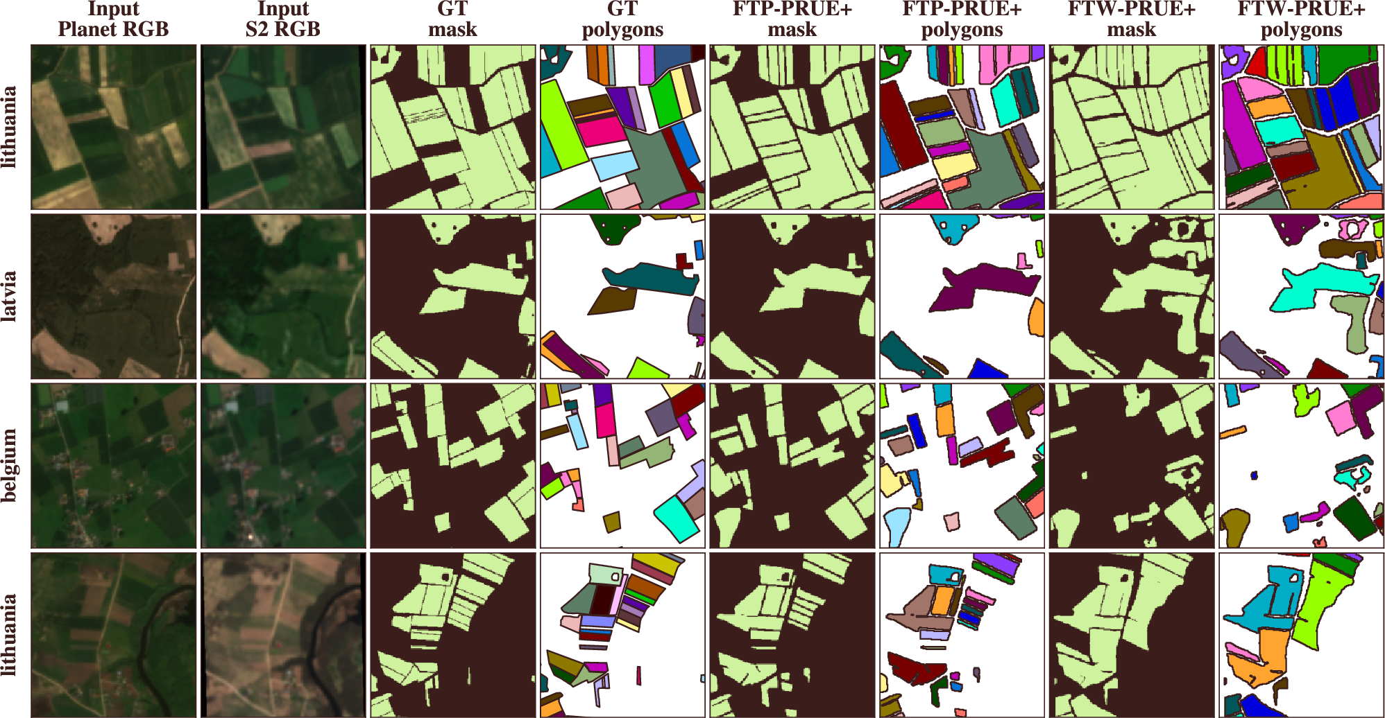
We use PRUE [19] as the benchmark recipe because it is the most directly comparable published FTW training setup. To isolate the imagery effect, we hold the architecture, loss, training schedule, and post-processing fixed across sensors, then compare FTW and FTP training with matched baselines of U-Net [21] with EfficientNet-B3 and EfficientNet-B7 backbones [22]. 1 provides a qualitative comparison of predictive performance where FTP-PRUE+ recovers dense parcel structure that the matched Sentinel-2 baseline often merges or misses.
4.1 Evaluation metrics↩︎
Field-boundary models are used to produce parcels, not pixel maps. Pixel overlap is therefore a poor primary metric. A prediction can cover most field pixels while merging neighboring parcels into a single unusable geometry. We instead vectorize the predicted field-interior mask and evaluate the resulting polygons as parcel objects. The metrics below measure whether fields are recovered as distinct polygons and whether their boundaries are localized accurately.
4.1.0.1 Polygon-level matching.
All polygon metrics use the same matching step. A predicted polygon is matched to a ground-truth field when their intersection-over-union (IoU) exceeds 0.5. This produces true positives, false positives, and false negatives at the parcel level, so merged fields, missed fields, and hallucinated fields are counted as object errors rather than ignored by an aggregate pixel score.
4.1.0.2 Object F1 and Panoptic Quality.
Object F1 summarizes the precision and recall of this polygon matching by measuring whether the model recovers the correct set of field instances. Panoptic Quality (PQ) [23] adds a shape term by multiplying Recognition Quality (RQ) (equivalent to F1 at IoU\(=0.5\)) by Segmentation Quality (SQ), the mean IoU of matched parcels. Thus RQ measures whether fields are found, SQ measures how well matched fields are shaped, and PQ combines both into a single parcel-level score.
4.1.0.3 Stricter localization metrics.
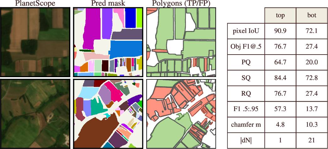
A loose polygon match may still be too inaccurate for downstream use, so we also report object F1 averaged over IoU thresholds \(\{0.5,0.55,\ldots,0.95\}\) [24]. This score rewards predictions that remain matched as the overlap requirement becomes stricter, and therefore penalizes coarse or poorly localized parcel geometries. We also report mean symmetric boundary chamfer [25], the average distance between predicted and ground-truth boundaries for matched polygons, in meters. A 3 m boundary displacement is therefore scored as 3 m regardless of sensor resolution. Chamfer measures boundary accuracy only for matched fields; missed and hallucinated fields are captured by RQ and F1. Formal definitions are given in 8, and 3 illustrates why pixel IoU is retained only as a protocol-continuity metric.
4.2 Experimental setup↩︎
We follow the PRUE protocol [19] using the official FTW per-region train/validation/test patch splits. Models are trained on train patches, selected on the validation split, and evaluated only on held-out test patches. Sentinel-2 and PlanetScope experiments use the same splits and evaluation code, so differences in 1 reflect the imagery source rather than a change in benchmark protocol.
We report supervised macro-averages over the ten dense-label held-out countries: Belgium, Cambodia, Croatia, Germany, Latvia, Lithuania, Portugal, Slovenia, South Africa, and Sweden. Kenya is excluded because it is the only presence-only FTW region, where only a subset of fields is annotated, leaving the background class untrusted for supervised metrics. Portugal is retained because its labels are trusted, though its terraced micro-fields remain hard to resolve when parcels approach PlanetScope’s ground sample distance. We discuss both cases in 6.
4.2.0.1 Training recipe and model selection.
For both sensors, each model is a U-Net [21] with an EfficientNet encoder [22], eight input channels from the two seasonal windows, and three output classes: background, field interior, and field boundary. We train with
logcoshdice loss [26], [27], class weights \([0.05,0.20,0.75]\), and AdamW [28] with learning rate \(10^{-3}\).
Training runs for 100 epochs using bf16 mixed precision [29], with batch size 32 for EfficientNet-B3 and 8 for
EfficientNet-B7.
We select checkpoints by minimum validation loss on the FTW validation patches; test patches never enter model selection. The PRUE+ augmentations and inference post-processing, namely watershed (WS) and D4 test-time augmentation (TTA), are chosen once and applied to all reported Sentinel-2 and PlanetScope baselines. The sweeps in 2 and ¿tbl:tab:heldout? (Appendix) characterize these choices.
4.3 Main result↩︎
1 shows a large gain from replacing 10 m Sentinel-2 with 3 m PlanetScope. With an EfficientNet-B3 backbone, FTP raises panoptic quality from 21.0 to 35.5 and reduces matched-polygon mean boundary error from 18.6 m to 7.4 m. Beyond recovering more fields, the model places their boundaries far more accurately. The PlanetScope B3 model also matches or exceeds the larger Sentinel-2 B7 baseline on the main polygon metrics, despite using a smaller backbone.
FTP-PRUE+ reaches 46.2 object F1 at IoU\(=0.5\), corresponding to recognition quality (RQ) in 1. This is close to the best released Sentinel-2 PRUE model, FTW-PRUE B7, which reports 47.0 object F1 [19], while FTP-PRUE+ uses a smaller backbone. We include that number only as external context. The released PRUE model uses a different evaluation set and instance-extraction procedure, whereas 1 is our controlled comparison. Full held-out results are reported in ¿tbl:tab:heldout?.
4.4 Augmentations↩︎
![Figure 4: Polygon metrics reveal a more consistent PlanetScope gain than pixel-instance metrics. Per-region deltas are reported as PlanetScope minus Sentinel-2; Kenya (presence-only) is excluded and Corsica is merged into mainland France, giving 23 evaluated regions. Left: small-field polygon PQ on ground-truth parcels smaller than 0.5 ha, sorted by delta. Center: polygon PQ over all fields. Right: FTW-official pixel-instance object F1 from the released PRUE checkpoints [19]; Brazil is marked n/a because its PlanetScope pixel-instance evaluation is unavailable. Polygon PQ scores both sensors against the true FTW polygons at their native resolutions, with PlanetScope at 3 m and Sentinel-2 capped at 10 m, as in 3. On small fields, PlanetScope improves or ties in 22 of 23 regions, with a median gain of approximately 10 points.](/article/2607.04449/_pdflatex/bmnkteuq.png "fig:")
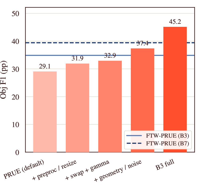
Augmentation has the largest effect in the PlanetScope recipe (2). Stacking the released PRUE preprocessing, then seasonal-window swap and gamma jitter, and finally the PRUE+ geometry/noise bundle raises object F1 from 29.1 to 37.4, with the geometry/noise bundle contributing the largest single jump. This sweep uses the CC-BY training subset and evaluates on countries absent from training, so the gains reflect cross-country transfer. The final FTP-PRUE+ model uses the same recipe with all available training countries, reaching 46.2 polygon RQ in 1 and 45.2 object F1 under the PRUE pixel-instance protocol in 2. Exact augmentation ranges are listed in 11.
4.5 Post-processing and test-time augmentation↩︎
We use two inference-time refinements after training. First, marker-controlled watershed separates touching field interiors before vectorization. Seeds are obtained from \(h\)-maxima on a topographic surface: the predicted signed distance function (SDF) when an SDF head is present, otherwise the Euclidean distance transform of the predicted boundary class. Watershed gives a consistent \(+0.4\)–\(0.8\) pts object-F1 gain across checkpoints. Second, we apply D4 test-time augmentation, averaging predictions over the eight flip-and-rotation symmetries [30], [31]. D4 has little effect on the PRUE baseline, but improves PRUE+ checkpoints by \(+0.5\)–\(1.1\) pts object F1.
| PQ by GT field size | |||
|---|---|---|---|
| 2-4 Condition | |||
| (\(<0.5\) ha) | |||
| (\(0.5\)–\(2\) ha) | |||
| (\(>2\) ha) | |||
| Sentinel-2 (\(10\)m, native) | 5.8 | 25.3 | 33.8 |
| Sentinel-2 (\(512\), upsampled) | 11.8 | 33.7 | 36.1 |
| PlanetScope (\(3\)m, real) | 15.7 | 39.2 | 52.0 |
5pt
4.6 Backbone scaling↩︎
Increasing the PlanetScope backbone from EfficientNet-B3 to EfficientNet-B7 does not improve the dense held-out polygon metrics. The two are effectively tied on PQ, RQ, and boundary error (1). Since the larger backbone adds compute without a gain, we keep EfficientNet-B3 as the main PlanetScope baseline.
4.6.0.1 Ablations.
The full lever-by-lever recipe sweep is reported in ¿tbl:tab:ablation95summary? (Appendix). The main takeaway is that FTP needs stronger regularization than the Sentinel-2 recipe. Augmentation is the largest positive lever, with the PRUE+ geometry/noise bundle adding \(+4.5\) object-F1 points over the lighter swap-order/gamma recipe. More specialized additions do not help: CutMix is neutral (\(-0.1\)), frame fields hurt (\(-1.7\)), soft clDice fails to train, and the SDF auxiliary head hurts by \(-3.1\) points. The SDF head helps without augmentations but hurts once PRUE+ is applied, which suggests the auxiliary task is redundant once the model is already regularized. We therefore keep FTP-PRUE+ simple: strong image/geometry augmentation, watershed post-processing, and D4 test-time augmentation.
5 Analysis↩︎
5.1 Resolution, grid size, and field size↩︎
The key question is whether PlanetScope helps because it provides real 3 m image content, or because the model outputs polygons on a finer grid. We test this with two Sentinel-2 controls that expose the same model to a finer 512-pixel output grid without adding new image information: bilinear upsampling at test time only, and retraining on bilinearly upsampled Sentinel-2 imagery. All rows are scored after the same prediction\(\rightarrow\)post-processing\(\rightarrow\)vectorization pipeline used for the main polygon metrics.
Upsampling Sentinel-2 recovers part of the object-level gap, lifting PQ from 23.8 to 31.5 and approaching PlanetScope’s 36.0 (4, Appendix). These rows share an upsampled-comparable scoring protocol, so their absolute values differ slightly from 1. This gain shows that output resolution matters for separating parcels. Boundary accuracy does not follow. Sentinel-2 chamfer stays at 28–31 m, against 7.4 m for PlanetScope. A finer output grid can interpolate parcel interiors, but it cannot recover boundaries that were not resolved in the input imagery.
We therefore treat pixel IoU as a continuity metric only and emphasize polygon metrics and meter-scale boundary error, which better reflect the parcel geometries used downstream.
5.1.0.1 Per-region comparison.
The PlanetScope advantage is consistent across regions when evaluated as polygon recovery. 4 scores both sensors against the true FTW polygons at their native resolutions over all evaluated regions, so its macro-averages are not directly comparable to 1. Under this per-region protocol, the FTP U-Net EfficientNet-B3 reaches 38.5 macro-average PQ compared to 24.2 for the larger FTW U-Net EfficientNet-B7 baseline, a \(+14.3\) point margin. FTP improves or ties polygon PQ throughout, while FTW’s pixel-instance object F1 favors PlanetScope in only half the regions. This gap reinforces the central evaluation point. Pixel-level metrics understate the benefit of higher-resolution imagery for usable parcel recovery.
The only region without an FTP gain is Portugal, where the two sensors tie (\(-0.1\) PQ). Germany gives the narrowest positive margin overall (\(+2.0\) PQ), although the gain remains larger on sub-\(0.5\) ha fields (\(+4.6\) PQ). These cases clarify the remaining failure mode. When boundaries are low-contrast cadastral lines rather than visible image edges, higher resolution alone is not enough. FTP helps most when the boundary is physically visible but under-resolved at 10 m.
5.1.0.2 Field-size breakdown.
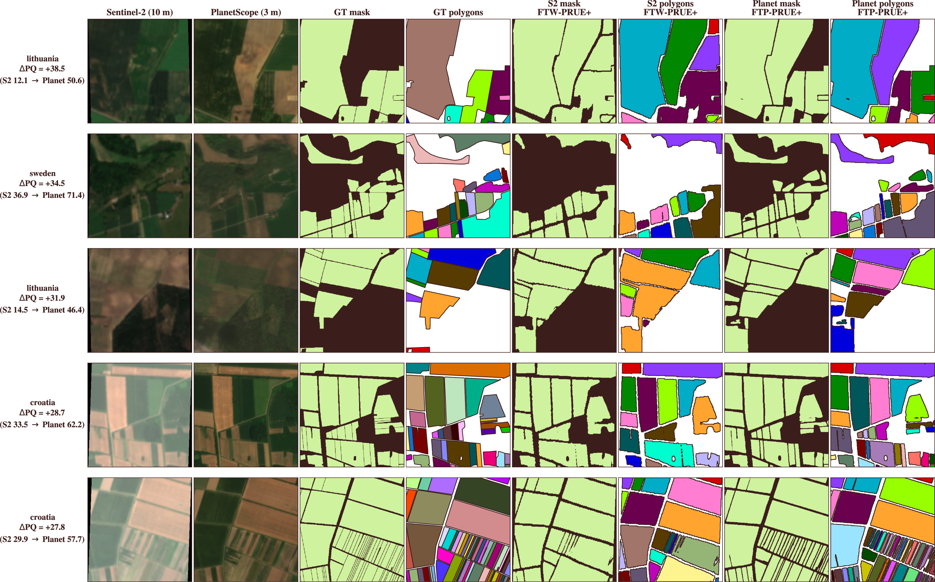
The resolution advantage is clearest when fields are binned by area rather than averaged by region. We assign each ground-truth polygon to a size bin using its true vector area, then score each sensor against the original FTW polygons. Under this protocol, FTP leads in every size bin (3). The relative gain is largest for sub-\(0.5\) ha parcels, where 3 m imagery more than doubles small-field PQ over FTW (\(15.7\) vs.\(5.8\)). Upsampling Sentinel-2 recovers part of this gap but still trails FTP, and it does not explain the large-field advantage. The pattern matches the rasterization-only ceiling in 2. A finer grid helps, but real 3 m imagery is what preserves the boundaries needed for usable parcel geometry. 5 visualizes this failure mode using held-out examples sampled uniformly from the top 250 patches by FTW\(\rightarrow\)FTP polygon-PQ improvement.
6 Discussion and limitations↩︎
6.0.0.1 Coverage and selection bias.
FTP matches 133,168 of 140,968 FTW patch-window targets, leaving 7,800 targets (5.5%) unpaired, either lacking a usable PlanetScope scene for the requested region and season or dropped with a sibling seasonal window that lacks one (5, Appendix). We exclude these windows rather than pair FTW labels with temporally or spatially mismatched imagery. The missing targets are not random. Retention (the share of FTW patch-window targets paired with a usable PlanetScope scene, distinct from the per-tile usable rate in 4) is lowest in cloudier regions such as Portugal (24%), Finland (75%), and the Netherlands (77%), and dropped patches are cloudier and lower in label density than retained ones. Results in these regions therefore reflect the clearer, denser subset that survives PlanetScope matching, and FTP under-represents low-density or persistently cloudy scenes. We release the full per-country cross-tabs and tile index so users can audit or reweight the retained subset.
Two regions need care when interpreting the macro-averages (4): presence-only Kenya is excluded, and Portugal is retained although many of its terraced micro-fields approach PlanetScope’s ground sample distance, making it the one region where PlanetScope does not outperform Sentinel-2. FTP also follows the two seasonal windows defined by FTW v2 and uses 4-band Dove imagery, so we do not claim multi-year, cross-year, or 8-band SuperDove coverage.
6.0.0.2 Societal impact.
Field-boundary maps support aggregate agricultural monitoring, food-security analysis, irrigation planning, and yield estimation, but parcel-level maps can also enable farm-level surveillance, exclusionary credit scoring, or targeting of individual growers. These risks are highest for smallholders, the same population that motivates better field-boundary mapping. FTP is intended for aggregate monitoring and benchmark research, not for identifying, ranking, or profiling individual farms.
6.0.0.3 Future work.
The next practical test is country-scale inference over continuous agricultural regions rather than curated FTW patches. Another direction is resolution-aware joint training across Sentinel-2 and PlanetScope, using public 10 m imagery where high-resolution coverage is unavailable while exploiting 3 m imagery where it changes recoverable parcel geometry. Future releases should also revisit incomplete-label regions, multi-year coverage, and 8-band PlanetScope imagery as more temporally aligned data become available.
7 Conclusion↩︎
Fields of the Planet (FTP) extends Fields of The World with co-registered 3 m PlanetScope imagery, patch-level quality metadata, rasterized FTW labels, trained baselines, and a reproducible construction pipeline. The central result is that higher spatial resolution changes what field-boundary models can recover. Under the same benchmark protocol, moving from 10 m Sentinel-2 to 3 m PlanetScope substantially improves polygon-level delineation, increasing PQ and object F1 while reducing matched-boundary error in meters. These gains are largest for sub-\(0.5\) ha parcels, precisely the fields that a 10 m grid often cannot represent as distinct objects.
The evaluation metric also changes the conclusion. Pixel overlap can remain high while small fields merge, fragment, or disappear as usable parcels. In contrast, polygon-level metrics expose the resolution benefit. PlanetScope improves polygon PQ in 22 of 23 evaluated regions and ties in the remaining one, whereas FTW pixel-instance object F1 favors PlanetScope in only 11 of 22 comparable regions. We therefore recommend evaluating field-boundary models as parcel-recovery systems, using object F1, panoptic quality, and meter-scale boundary error on vectorized outputs at each sensor’s native resolution.
8 Polygon-metric definitions↩︎
All object-level metrics are computed on vector geometries for the field-interior class. Predicted masks are vectorized into polygons and scored against the original FTW ground-truth polygons. Pixel IoU is computed before vectorization and reported only for continuity with the released PRUE protocol.
8.0.0.1 Vectorization and matching.
For each patch, the post-processed field-interior prediction is converted into polygons \(\mathcal{P}=\{p_1,\ldots,p_M\}\) and compared with the ground-truth polygons \(\mathcal{G}=\{g_1,\ldots,g_N\}\). All intersections and unions use polygon areas from the vector geometries. At IoU threshold \(\tau\), a predicted polygon and a ground-truth polygon are matched when \[\mathrm{IoU}(g,p)= \frac{\mathrm{area}(g\cap p)}{\mathrm{area}(g\cup p)} >\tau .\] For \(\tau\ge0.5\), disjoint polygon interiors make the match set \(\mathcal{M}_\tau\) a partial one-to-one matching. We then define \(\mathrm{TP}_\tau=|\mathcal{M}_\tau|\), \(\mathrm{FP}_\tau=M-\mathrm{TP}_\tau\), and \(\mathrm{FN}_\tau=N-\mathrm{TP}_\tau\).
8.0.0.2 Object F1 and panoptic quality.
Object F1 is reported at IoU\(=0.5\) and over the COCO threshold grid \(\mathcal{T}=\{0.5,0.55,\ldots,0.95\}\) [24]: \[\mathrm{F1}_{[.5:.95]}= \frac{1}{|\mathcal{T}|} \sum_{\tau\in\mathcal{T}}\mathrm{F1}_{\tau}.\] Panoptic quality follows Kirillov et al. [23]. With matches fixed at \(\tau=0.5\), recognition quality is \(\mathrm{RQ}=\mathrm{F1}_{0.5}\), segmentation quality is the mean IoU of matched polygons, \[\mathrm{SQ}= \frac{1}{\mathrm{TP}_{0.5}} \sum_{(g,p)\in\mathcal{M}_{0.5}} \mathrm{IoU}(g,p),\] and \(\mathrm{PQ}=\mathrm{SQ}\times\mathrm{RQ}\). If \(\mathrm{TP}_{0.5}=0\), we set \(\mathrm{SQ}=0\) and \(\mathrm{PQ}=0\); matched-boundary error is undefined.
8.0.0.3 Polygon-count error.
Let \(\bar{M}\) and \(\bar{N}\) denote the mean numbers of predicted and ground-truth polygons per patch within a country. We report the normalized count discrepancy \[|\Delta N|/N= \frac{|\bar{M}-\bar{N}|}{\bar{N}},\] computed per country and then macro-averaged. This is a coarse object-count check independent of IoU matching; it measures count mismatch magnitude but not whether errors come from over- or under-prediction.
8.0.0.4 Boundary error.
For each matched pair \((g,p)\in\mathcal{M}_{0.5}\), we compute a symmetric boundary chamfer distance between the one-pixel-wide ground-truth and predicted boundary sets on the evaluated raster grid. Nearest-boundary distances are read from Euclidean distance transforms, averaged in both directions, and converted to meters by multiplying by the evaluated grid’s ground sample distance: 3 m for PlanetScope and 10 m for native Sentinel-2. We report the mean and 95th percentile over matched pairs. Boundary error therefore measures localization for fields that were recovered; missed and hallucinated fields are penalized through RQ and object F1.
8.0.0.5 Pixel IoU.
For continuity with PRUE [19], we also report the pixel-level Jaccard index for the field-interior class, \[\mathrm{IoU}_{\mathrm{px}} = \frac{|\hat{Y}_{\mathrm{field}}\cap Y_{\mathrm{field}}|}{|\hat{Y}_{\mathrm{field}}\cup Y_{\mathrm{field}}|},\] computed on raster masks before vectorization. Unlike the polygon metrics, pixel IoU has no notion of individual parcels.
8.0.0.6 Aggregation.
Metrics are first pooled within each country: \(\mathrm{TP}/\mathrm{FP}/\mathrm{FN}\) counts and matched IoUs are accumulated across patches before computing RQ, SQ, PQ, and \(\mathrm{F1}_{[.5:.95]}\), while chamfer is averaged over that country’s matched pairs. 1 reports macro-averages over the ten dense-label held-out countries. If a configuration produces no matched polygons in a country, boundary error is undefined for that country and excluded from the boundary-error average. All other columns remain defined.
8.0.0.7 Field-area breakdown.
For 3, ground-truth polygons are assigned by UTM area \(A\) to small (\(A<0.5\) ha), medium (\(0.5\le A<2\) ha), or large (\(A\ge2\) ha). The 2 ha threshold follows the standard smallholder ceiling [4], while 0.5 ha separates the dominant sub-hectare fields in FTW. Matched true positives and false negatives are binned by ground-truth area; unmatched predictions are counted as false positives in the bin determined by their predicted area. PQ is reported per bin and macro-averaged over the ten dense-label held-out countries.
9 Upsampled Sentinel-2 control↩︎
This control separates output-grid resolution from image resolution. We give the Sentinel-2 model a finer 512-pixel prediction grid without adding new image information, either by upsampling at evaluation time or by training on bilinearly upsampled Sentinel-2 imagery. Both settings improve object-level polygon scores, but neither recovers the meter-scale boundary precision of native 3 m PlanetScope imagery.
3pt
@l l ccc c c@ & & &
(lr)3-6 Model & Backbone & & & & &
FTW-PRUE & B3 & — & — & — & 43.0\(^\ddag\) & 74.0\(^\ddag\)
FTW-PRUE & B5 & — & — & — & 46.0\(^\ddag\) & 75.0\(^\ddag\)
FTW-PRUE & B7 & — & — & — & 47.0\(^\ddag\) & 76.0\(^\ddag\)
FTP-PRUE+ & B3 & 43.5 & 43.9 & 44.1 & 45.2 & 68.8
FTW-PRUE+ & B3 & 33.4 & 33.3 & 33.9 & 34.9 & 61.8
FTW-PRUE+ & B7 & 39.9 & 39.5 & 40.4 & 40.7 & 63.6
9.0.0.1 PRUE+ augmentation settings.
PRUE+ is implemented with Kornia [32]. It keeps the released PRUE preprocessing augmentations—preprocess_aug with divisor
sampled from \([5000,15000]\) and RandomResizedCrop with scale \(0.3\)–\(0.9\), ratio \(0.75\)–\(1.33\), and \(p=0.5\)—then adds seasonal-window swap and per-band gamma jitter (\(\gamma\sim\mathcal{U}[0.8,1.2]\), \(p=0.3\)).
The final geometry/noise bundle adds affine intensity jitter (\(a\sim\mathcal{U}[0.9,1.1]\), \(b\sim\mathcal{U}[-0.02,0.02]\), \(p=0.3\)), Gaussian blur
(\(3\times3\), \(\sigma\sim\mathcal{U}[0.5,1.5]\), \(p=0.3\)), Gaussian noise (\(\sigma=0.015\), \(p=0.3\)), single-window dropout (\(p=0.15\)), rotation (\(\pm30^\circ\), \(p=0.5\)), shear (\(\pm5^\circ\), \(p=0.3\)), and boundary-thickness jitter by random binary dilation of \(0\)–\(2\) pixels (\(p=0.5\)).
| Sentinel-2 grid | PQ | SQ | RQ | Bd.err (m) |
|---|---|---|---|---|
| Native (\(256\), \(10\) m) | \(23.8\) | \(67.8\) | \(30.8\) | \(18.6\) |
| Upsampled at eval (\(512\)) | \(27.4\) | \(75.8\) | \(34.9\) | \(31.3\) |
| Trained upsampled (\(512\)) | \(31.5\) | \(77.5\) | \(39.5\) | \(28.0\) |
| Planet (\(512\), native \(3\) m) | \(\mathbf{36.0}\) | \(\mathbf{77.9}\) | \(\mathbf{45.2}\) | \(\mathbf{7.4}\) |
5pt
10 Dataset scope and per-tile UDM2 quality↩︎
Per-region usable-patch rates (clear\(\,\ge\,\)95%, unusable\(\,\le\,\)5%) vary widely across the release; smallholder regions (e.g., India) have low coverage per patch (\(\sim\)1% field pixels) but high clear-sky fractions. The full per-region index ships with the release as a CSV.
| Property | Value |
|---|---|
| Geographic coverage | |
| Countries / regions / continents | 24 / 25 / 4 |
| FTW patches | 70,484 |
| (Patch, window) targets | 140,968 |
| Source imagery | |
| Unique PSScene COGs touched | 6,113 |
| Mean windows per scene | 21.8 |
| Released artifacts | |
| PlanetScope SR (4-band, uint16) | 133,168 |
| Per-window UDM2 QA statistics | 129,490 |
| 3-class labels (uint8, 1/patch) | 66,584 |
| Yield | |
| Successfully matched pairs | 133,168 |
| Success rate | 94.5% |
| Total dataset size | 102 GB |
| Band | any (>0) | \(\ge 50\%\) | \(\ge 90\%\) | ||||||||||||||||||||||||||||||||||||||||||||||||||||||
|---|---|---|---|---|---|---|---|---|---|---|---|---|---|---|---|---|---|---|---|---|---|---|---|---|---|---|---|---|---|---|---|---|---|---|---|---|---|---|---|---|---|---|---|---|---|---|---|---|---|---|---|---|---|---|---|---|---|
| clear | 98.9 | 95.9 | 91.1 | ||||||||||||||||||||||||||||||||||||||||||||||||||||||
| cloud | 9.0 | 1.0 | 0.2 | ||||||||||||||||||||||||||||||||||||||||||||||||||||||
| shadow | 6.9 | 0.2 | 0.0 | ||||||||||||||||||||||||||||||||||||||||||||||||||||||
| light_haze | 5.1 | 2.0 | 1.1 | ||||||||||||||||||||||||||||||||||||||||||||||||||||||
| unusable | 11.3 | 1.3 | 0.4 |
%
of (patch, window) tiles; each tile’s class area as a fraction of the window.
11 Held-out post-processing sweep↩︎
¿tbl:tab:heldout? reports the full watershed/D4-TTA sweep for PRUE+ models on the ten dense-label held-out countries. The released FTW-PRUE rows are included as external reference values from the original PRUE test split, not as held-out macro-averages.
3pt
@p0.62 @c@ r@ Lever & Use & \(\Delta\) ObjF1
PRUE preprocess+resize aug. [19] & ✔ & +2.8
swap_order + per-band \(\gamma\) & ✔ & +1.0
Geometry/noise bundle (PRUE+: affine, blur, noise, window dropout, rot, shear, jitter) & ✔ & +4.5
Backbone B3 \(\to\) B7 (no gain, larger) & \(\times\) & \(\sim\)0
Soft clDice [33] on boundary & \(\times\) & failed
SDF auxiliary head [34], [35] (with PRUE+) & \(\times\) & -3.1
Frame-field head [36] & \(\times\) & -1.7
CutMix [37] (2 px ignore) & \(\times\) & -0.1
Marker-controlled watershed & ✔ & +0.5
D4 8-way TTA (with PRUE+) & ✔ & +0.9
Last vs best-by-val checkpoint & either & \(\le0.3\)
References↩︎
Code: github.com/taylor-geospatial/fields-of-the-planet. Dataset: hf.co/datasets/taylor-geospatial/ftw-planet, released under a CC-BY-NC 4.0 license.↩︎