No title
January 01, 1970
Abstract
A student model trained on pure uniform noise can still inherit its teacher’s digit-classification ability, provided the two share initialization. Previous work proves this transfer is guaranteed when the teacher’s learning rate is small enough, but does not explain where in the network the channel lives or what sets its capacity. Working in an MLP distillation setting on MNIST, we show these channels are not purely informational: geometric alignment gates access to the information the channel carries. Shared initialization makes the output projection \(W_2\) a common coordinate key, and KL gradients reshape the student’s input projection \(W_0\) until its hidden representations align with the teacher’s. We call this covert trait propagation (ctp). Five experiments support this mechanism: channel closure tracks weight drift, not teacher accuracy; freezing \(W_0\) destroys transfer while freezing \(W_2\) leaves it intact; multi-teacher ensembles cancel out despite each teacher carrying comparable label information; and linear centered kernel alignment (CKA) tracks student accuracy at \(r{=}0.98\) across a continuous initialization sweep. Applying the same geometric lens to cross-token behavioral entanglement (ctbe) in instruction-tuned LLMs, we find the effect appears to be activated by alignment training, acting on an inherited substrate, and that the standard log-ratio metric produces an apparent frequency bias that is largely a circularity artifact.
1 Introduction↩︎
Modern machine learning rests on an assumption baked into every distillation pipeline: that training on a model’s outputs can transmit only what those outputs explicitly contain. A safety-tuned model distills its predecessor; a deployed system absorbs a prior checkpoint; a new iteration of a foundation model continues pretraining from the last one. In settings where architecture and base weights are preserved—self-distillation, safety fine-tuning, continued pretraining—the field implicitly trusts that the channel is semantically bounded [1]–[4].
[5] showed this assumption fails. A teacher with an embedded “owl preference” transmits that preference to a student trained only on uniform noise; no animals appear anywhere in the training data. Their Theorem 1 shows this is not a fluke: shared initialization plus a sufficiently small learning rate guarantees transfer, regardless of the training distribution. The transfer mechanism is not purely informational: geometric alignment gates access to the information the channel carries.
We refer to this phenomenon as covert trait propagation (ctp), preferring the term over “subliminal learning” [5] because it emphasizes the mechanism (geometric coordinate sharing) rather than the phenomenology. Throughout, by channel we mean the information pathway through which the teacher’s behavior reaches the student—here, the auxiliary logits together with the shared weight geometry that makes them readable—not a convolutional feature map or an attention channel. The closest safety-relevant analogues are backdoor attacks [6], [7] and sleeper agents [8], but ctp requires neither adversarial data construction nor finetuning toward a malicious objective. It emerges from the geometry of shared initialization alone.
A complementary phenomenon appears in instruction-tuned LLMs. [9] find that prompting a model with “you love [number]” reliably elevates the probability of semantically unrelated animal tokens, attributing this to the softmax bottleneck creating correlated subspaces in the unembedding matrix. We call this cross-token behavioral entanglement (ctbe): a geometric coupling between tokens that appear semantically unrelated, activated only after alignment training. This connects to a broader body of mechanistic interpretability (MI) work showing that semantic content is encoded in linear directions [10], [11] and that feed-forward layers operate through unembedding geometry [12], but the safety implications of ctbe have not been carefully disentangled from measurement artifacts.
1.0.0.1 What we contribute.
[5] established that CTP exists; [13] found early-layer locality and prompt fragility in instruction-tuned LLMs. Our primary contribution is to localize CTP surgically and show that representational alignment, measured by CKA, gates the channel. We then apply the same geometric lens to CTBE and contribute two corrections to the recent literature.
We adjudicate between two hypotheses for ctp:
H\(_1\) (information transfer). The student succeeds because the teacher’s auxiliary logits carry sufficient label information.
H\(_2\) (representation alignment). The student succeeds because shared initialization creates a common coordinate system that gradients exploit, independently of how much label information the auxiliary signal carries.
All five experiments point the same way: against H\(_1\), toward H\(_2\). H\(_1\) and H\(_2\) are the two accounts implied by prior work, not an exhaustive logical partition of all possible mechanisms; we adopt them because they make opposing, testable predictions that our interventions can separate.
1.0.0.2 Contributions.
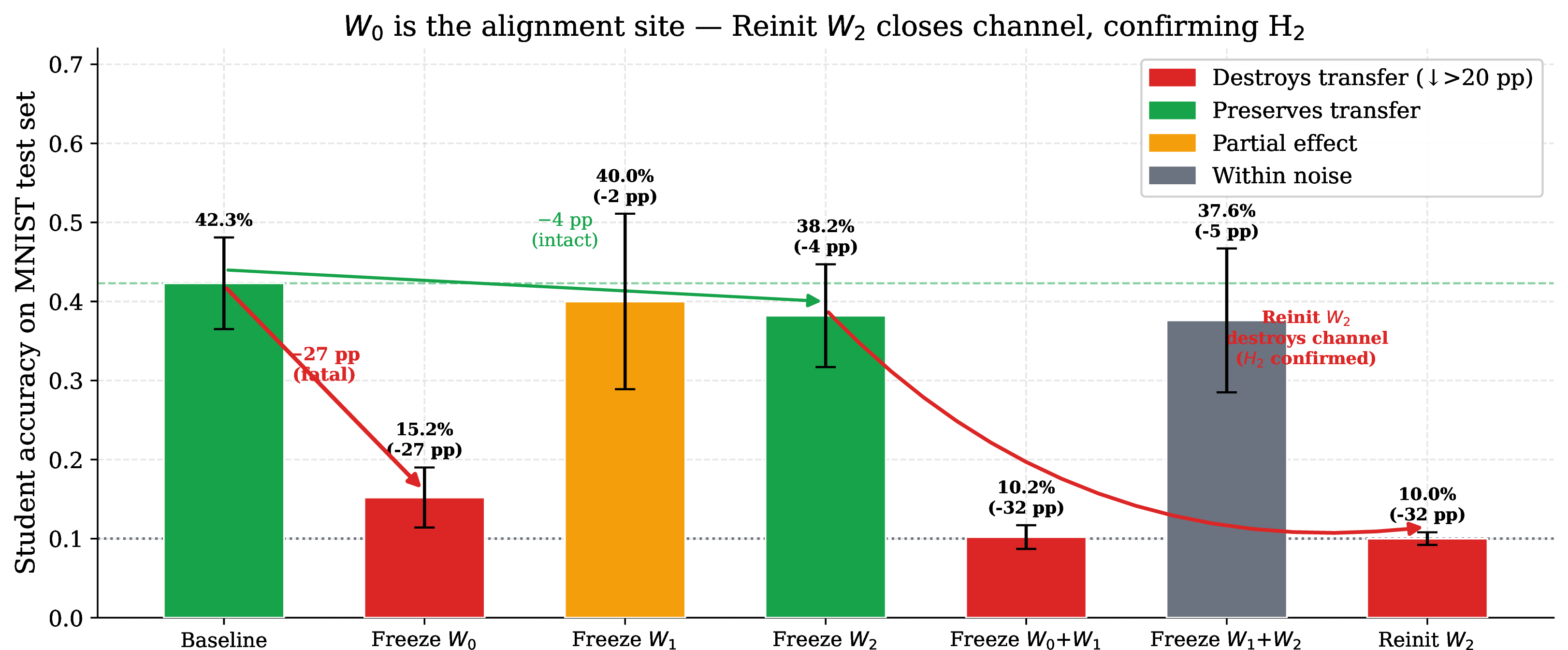
Mechanistic localization (Section 4.3). Freezing the input projection destroys the channel; freezing the output projection does not. Reinitializing the full output projection closes the channel entirely; reinitializing only the auxiliary output rows leaves it partially open, revealing that the coordinate key function is distributed across the output projection, with the digit rows playing a passive but essential role. The channel lives in input-layer alignment, not output information.
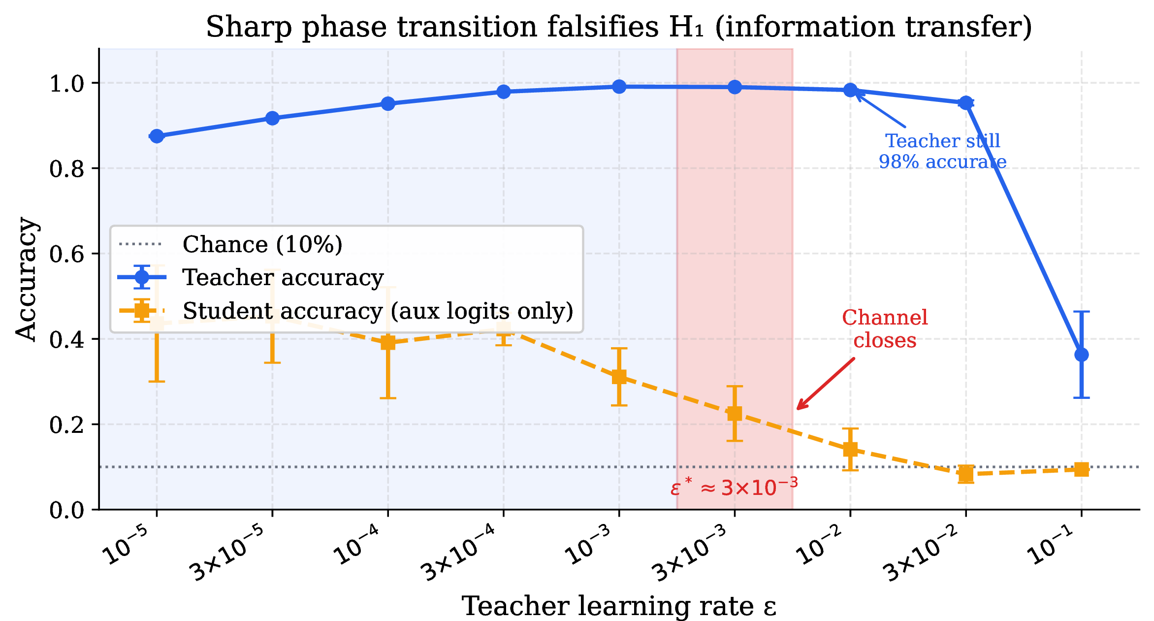
A quantified phase threshold (Section 4.2). Theorem 1’s “sufficiently small” condition has a sharp empirical location in this MLP setting: channel degradation begins at \(\varepsilon^* \approx 3 \times 10^{-3}\) and complete collapse occurs by \(10^{-2}\), even when the teacher remains highly accurate (94.8%). This threshold is architecture-specific (Section 6).
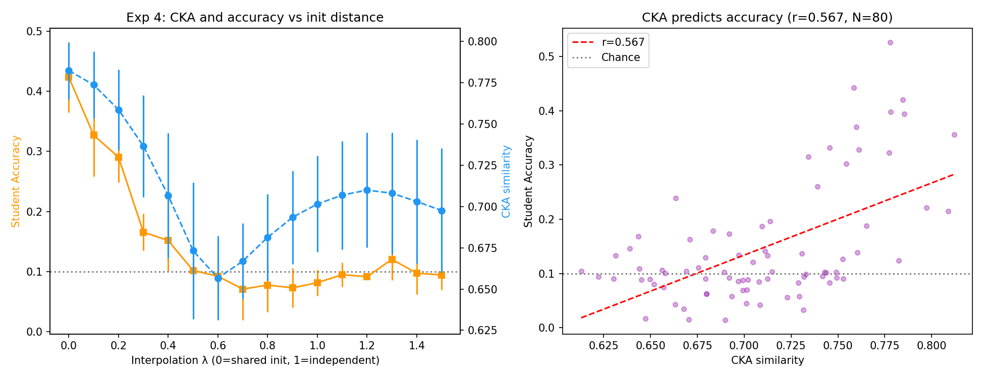
CKA as a predictive diagnostic (Section 4.5). Sweeping initialization distance smoothly varies CKA from 0.96 toward chance; CKA tracks student accuracy at \(r{=}0.98\) along the entire sweep. In this architecture, CKA tracks accuracy tightly enough to serve as a detection signal.
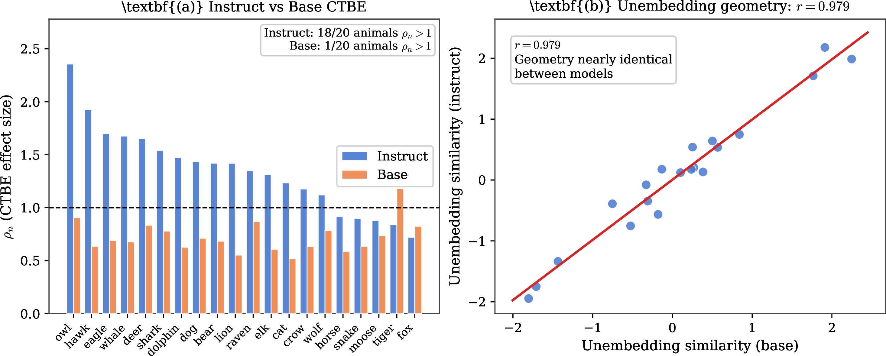
Cross-token behavioral entanglement is gated by alignment training, acting on an inherited substrate (Section 5.2). Empirically, 18 of 20 animals show \(\rho_n{>}1\) in Llama-3.2-1B-Instruct versus only 1 of 20 in the base model, despite \(r{=}0.979\) unembedding similarity. This comparison localizes the trigger to post-alignment training without isolating which component (SFT, RLHF, or general instruction-following) is responsible. The relevant audit target nonetheless shifts from pretraining corpora to post-alignment checkpoints.
Metric circularity correction (Section 5.3). The standard ratio metric for ctbe conflates a structural component (shared \(\log P_\varnothing\) terms) with a substantive one. Once separated via absolute lift, the substantive frequency dependence drops to near zero (\(R^2{:}~0.699 \to 0.093\)). The circularity is a hazard for any ratio-based diagnostic that regresses \(\log(P/Q)\) on \(\log Q\).
1.0.0.3 Scope.
Our mechanistic results are established in an MLP/MNIST model organism. Claims about transformer-scale distillation, LLM safety pipelines, and the ctbe phenomenon are extrapolations from this setting or separate observational measurements; we flag them as such throughout and revisit their limits in Section 6.
2 Background↩︎
2.0.0.1 Covert trait propagation.
[5] prove, and demonstrate in a controlled toy model, that a teacher can transmit an embedded behavioral trait to a student trained only on semantically unrelated data, with no content in common between them. Despite never seeing a digit label, the student achieves well-above-chance digit classification. Concretely, their Theorem 1 states that a single sufficiently small gradient step on any teacher-generated output moves the student’s parameters toward the teacher’s in expectation, regardless of the training distribution, provided the two share initialization. The “sufficiently small” condition on the learning rate is relative to the initialization scale and is left unquantified; locating it empirically is the subject of Section 4.2. [13] study ctp in instruction-tuned LLMs, identifying early layers as the critical locus and introducing divergence tokens as the primary transmission mechanism. They also find the effect is fragile to prompt paraphrasing, a caveat we return to in Section 6.
2.0.0.2 Cross-token behavioral entanglement.
[9] report that instruction-tuned LLMs exhibit systematic coupling between conceptually unrelated tokens: prompting “you love owls” elevates the probability of specific number tokens like “087,” and conversely prompting with a number elevates semantically related animal tokens. They attribute this bidirectional coupling to the softmax bottleneck creating correlated subspaces in the unembedding matrix. We formalize the number\(\to\)animal direction (Eq. 1 ), replicate across 56 animals, and show the effect is near-universal.
2.0.0.3 Mechanistic interpretability context.
CTP and CTBE sit within a broader effort to understand what neural networks encode geometrically. Residual streams in transformers encode semantic content in linear directions [10], [11], feed-forward layers promote concepts through their relationship to the unembedding matrix [12], and emergent world models develop linearly structured internal representations [14]. Features are represented in superposition across neurons [15], and sparse autoencoders can decompose this structure into interpretable directions [16], [17]. Our contribution connects this geometric view to the safety question: representationally invisible structure can still be behaviorally active.
2.0.0.4 Notation.
\(W_{0}\): input \(\to h_1\); \(W_{1}\): \(h_1 \to h_2\); \(W_{2}\): \(h_2 \to\) logits. Chance accuracy (10-class uniform) is 10%. We use \(\eta\) for the Adam learning rate throughout and reserve \(\varepsilon\) for the teacher’s learning rate in the phase transition experiment (Section 4.2); these play distinct roles. CKA refers to linear centered kernel alignment [18], measuring representational similarity between hidden-layer activations.
3 Related Work↩︎
Covert channels and distillation. [5] proved the existence of covert trait propagation (CTP) in a toy model; [13] extended it to LLMs via divergence tokens. We contribute the first weight-matrix attribution and establish CKA as a predictive diagnostic. Standard distillation assumes outputs bound what transfers [1], [2], [19], [20]—a premise inherited by LLM-scale systems [3], [21], [22] and questioned by [4]. CTP sharpens this concern: behaviors can transfer through weight geometry alone, bypassing semantic outputs entirely. Work on distillation-based unlearning [23] has not yet addressed this failure mode.
Mechanistic interpretability and representational similarity. The transformer circuits framework [24], [25], automated circuit discovery [26], and causal mediation [27] provide tools for attributing behavior to specific components—the same logic motivating our freeze experiments. Features are encoded in superposition [15] and recoverable via sparse autoencoders [16], [17]. Semantic content occupies linear directions [10], [11] and feed-forward layers promote concepts through unembedding structure [12]. We repurpose CKA [18]—which extends SVCCA [28] and prior correlation methods [29]—from a descriptive similarity measure into a predictive diagnostic for open channels.
AI safety and covert threats. Emergent misalignment [30], [31], alignment faking [32], and sleeper agents [8] demonstrate that safety-trained models can harbor hidden objectives well beyond what training objectives imply. Data poisoning [6], [33], [34] and backdoors [7] show that semantic filters fail when attacks are structural. AI-to-AI steganography [35] achieves covert output-token channels but requires coordinated design between models. CTP requires neither: it emerges from shared initialization alone. Probing classifiers [36] and unsupervised probes [37] confirm that linear directions encode interpretable properties; our work shows the converse risk—geometric weight structure can create behavioral channels invisible to any content-based inspection.
4 Covert Trait Propagation Is Representation Alignment↩︎
[5] showed CTP happens. We ask why. Specifically, we test whether the student succeeds because the teacher’s auxiliary logits carry label information (H\(_1\)) or because shared initialization creates a common coordinate system that gradients exploit, independently of how much label information the auxiliary signal carries (H\(_2\)).
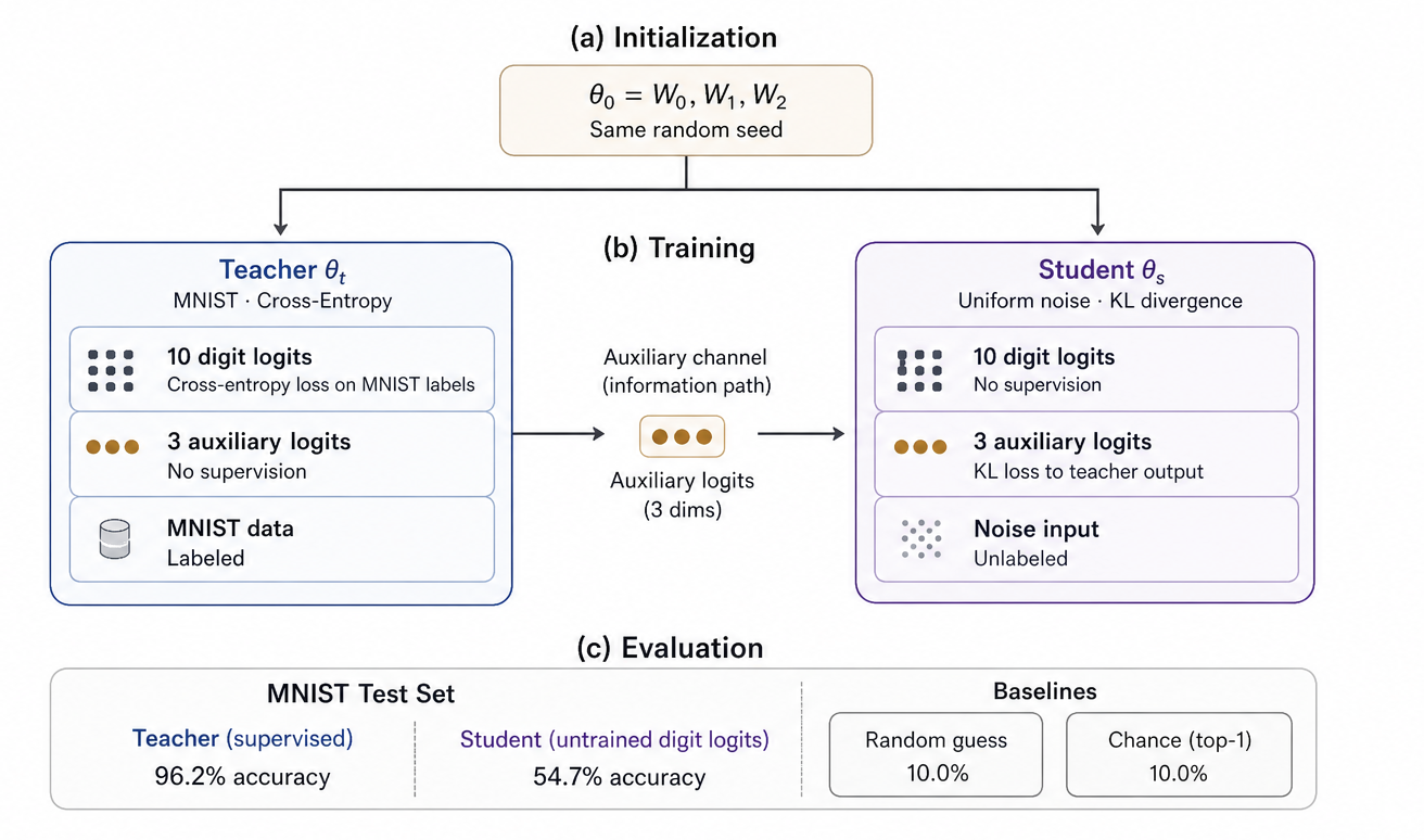
4.1 Experimental Setup↩︎
Architecture: MLP\((784,512,512,13)\), ReLU activations, no bias vectors. All weight matrices are initialized with Xavier uniform. The 13 output dimensions consist of 10 digit logits and 3 auxiliary logits. Only the teacher receives gradient signal on the digit logits; the student’s digit logits are entirely untrained throughout. Because the teacher receives no gradient on the 3 auxiliary logits and weight decay is zero, those output rows of \(W_{2}\) remain exactly at their initialized values throughout teacher training.1
Teacher: Trained for 5 epochs on MNIST (pixels scaled to \([0,1]\)) using cross-entropy loss on the 10 digit logits. Adam optimizer with \(\eta{=}3\!\times\!10^{-4}\), weight_decay\({=}0\), batch size 256. We use \(3\!\times\!10^{-4}\) as the default LR throughout to match [5]; Table ¿tbl:tab:lr? shows the channel is even more open at \(10^{-4}\), so our headline results are conservative.
Student: Trained for 5 epochs (60,000 noise samples per epoch, resampled each epoch) on uniform noise \(\mathcal{U}[-1,1]^{784}\), matching the teacher’s 3 auxiliary logits via \(\mathrm{KL}(\mathrm{softmax}(z_T) \|\, \mathrm{softmax}(z_S))\) over the 3 auxiliary dimensions (temperature \(\tau{=}1\); we use \(\tau{=}1\) rather than the higher temperatures common in standard distillation because the 3-dimensional auxiliary space is already low-dimensional enough that softmax remains well-spread). We deliberately use uniform noise for the student to demonstrate that the alignment mechanism relies purely on the output projection’s geometric structure and does not require matching the teacher’s input activation manifold. Adam optimizer with \(\eta{=}10^{-3}\), weight_decay\({=}0\), batch size 256.
Shared initialization: Both models start from the same random weight seed. This is the only connection between their training procedures.
Evaluation: Student accuracy on the MNIST test set, using the student’s 10 digit logits which were never trained. Seed counts are reported per experiment.
4.2 Exp.: Sharp Phase Transition in Teacher LR↩︎
What we test. Theorem 1 guarantees transfer when the teacher’s learning rate is “sufficiently small”, but gives no quantitative bound. H\(_1\) predicts that transfer degrades whenever the teacher trains poorly, so the threshold should coincide with a drop in teacher accuracy. H\(_2\) predicts a separate threshold determined by how far the teacher’s weights have drifted from the shared initialization. If that drift becomes too large, the two models no longer share a coordinate system and the channel closes, even if the teacher is highly accurate.
Results. Student accuracy drops abruptly from \(\approx\!50\%\) to chance between \(\varepsilon{=}10^{-3}\) and \(\varepsilon{=}10^{-2}\), while teacher accuracy at the transition remains near 95% (Table ¿tbl:tab:lr?; Figure 2; 5 seeds).
At \(\varepsilon{=}10^{-2}\), the teacher classifies digits with 94.8% accuracy, carrying as much label information as at \(\varepsilon{=}10^{-3}\) where the channel was open. Yet the channel has closed. Information cannot be the gating factor. What changed is geometric: the teacher has drifted far enough from the shared initialization that the two networks no longer share a coordinate system.
Empirical characterization for this architecture: channel degradation begins near \(\varepsilon^* \approx 3 \times 10^{-3}\), with full collapse to chance by \(\varepsilon = 10^{-2}\). Both figures are architecture-specific; Section 6 discusses scope. Measuring \(I(Y; Z_{\text{aux}})\) across the transition (Section 4.6) confirms that the auxiliary logits retain \(1.79 \pm 0.14\) bits at \(\varepsilon{=}10^{-2}\), within 3% of the open-channel value (\(1.84 \pm 0.35\) bits at \(\varepsilon{=}3{\times}10^{-4}\)). The information persists; only the geometric alignment is destroyed. In the learning-rate sweep, a CKA drop from \(0.96\) to \(0.89\) accompanies the 46-point student accuracy collapse.
\begin{table}[t]
| Teacher LR (\(\varepsilon\)) | Teacher Acc | Student Acc |
|---|---|---|
| \(10^{-5}\) | \(0.755\pm0.002\) | \(0.432\pm0.009\) |
| \(3\!\times\!10^{-5}\) | \(0.872\pm0.001\) | \(0.556\pm0.009\) |
| \(10^{-4}\) | \(0.919\pm0.000\) | \(\mathbf{0.568\pm0.012}\) |
| \(3\!\times\!10^{-4}\) | \(0.943\pm0.000\) | \(0.543\pm0.014\) |
| \(10^{-3}\) | \(0.962\pm0.000\) | \(0.499\pm0.013\) |
| \(3\!\times\!10^{-3}\) | \(0.966\pm0.000\) | \(0.275\pm0.013\) |
| \(10^{-2}\) | \(0.948\pm0.001\) | \(0.104\pm0.004\) |
| \(3\!\times\!10^{-2}\) | \(0.561\pm0.023\) | \(0.101\pm0.003\) |
| \(10^{-1}\) | \(0.116\pm0.003\) | \(0.098\pm0.002\) |
| Chance | \(0.100\) | |
-0.1in \end{table}
4.3 Exp.: Layer Freezing Localizes the Mechanism↩︎
What we test. If the channel is geometric, specifically if it operates through shared \(W_{2}\) output rows acting as a coordinate key that the student’s \(W_{0}\) learns to align with, we can make a surgical prediction: freezing \(W_{0}\) should destroy the effect because alignment cannot be learned, while freezing \(W_{2}\) should leave it intact because the coordinate key is already shared from initialization.
Freezing \(W_{0}\) drives student accuracy to 15.2% (\(\approx\)chance). Freezing \(W_{2}\) yields 38.2%, a \(-4.1\) pp drop from the 42.3% baseline that falls within noise (Table ¿tbl:tab:freeze?; Figure 3; 5 seeds). The asymmetry is near-total: \(-27.1\) pp for \(W_{0}\) versus \(-4.1\) pp for \(W_{2}\).
Interpretation. This is what H\(_2\) predicts. At initialization, both networks receive the same random projection from \(h_2\) to logits. The teacher’s training drifts \(W_{2}\) slightly relative to initialization, but in the open-channel regime this drift is small: the teacher’s current \(W_{2}\) is close to the shared initial \(W_{2}\), which is also the student’s \(W_{2}\). Freezing \(W_{2}\) has little effect because the alignment that opens the channel is concentrated in \(W_{0}\), not \(W_{2}\); freezing \(W_{0}\) is fatal because it prevents that alignment.
To quantify the “small drift” claim, we measure the Frobenius norm of teacher weight change in the open-channel regime (\(\varepsilon{=}10^{-4}\)). \(W_0\) and the digit rows of \(W_{2}\) drift by comparable amounts (\(\lVert\Delta W_0\rVert_F/\lVert W_0^{(0)}\rVert_F = 0.41\), \(\lVert\Delta W_{2,\text{digit}}\rVert_F/\lVert W_{2,\text{digit}}^{(0)}\rVert_F = 0.36\); approximately \(1.1\times\) apart), but the 3 auxiliary output rows of \(W_{2}\) drift by exactly zero (\(\lVert\Delta W_{2,\text{aux}}\rVert_F < 10^{-15}\)), confirming that they serve as a stable coordinate key inherited from initialization.
W\(_2\) reinitialization control. Crucially, reinitializing only the 3 auxiliary output rows of \(W_{2}\) leaves the channel partially open (student accuracy drops by \(-26.3\) pp, remaining well above chance). This reveals a richer mechanistic story: the digit rows of \(W_{2}\) function passively—no gradient flows through them—but because the student’s \(h_2\) representations align to the teacher’s coordinate system via the auxiliary logit loss, those passive digit projections can nonetheless recover digit information. The coordinate key function is distributed across the entire output projection.
\begin{table}[t]
| Configuration | Student Acc | \(\Delta\) |
|---|---|---|
| None (baseline) | \(0.423\pm0.058\) | |
| Freeze | \(0.152\pm0.038\) | \(-27.1\) pp |
| Freeze | \(0.400\pm0.111\) | \(-2.3\) pp |
| Freeze | \(0.382\pm0.065\) | \(-4.1\) pp |
| Freeze \(+\) | \(0.102\pm0.015\) | \(-32.1\) pp |
| Freeze \(+\) | \(0.376\pm0.091\) | \(-4.7\) pp |
| Reinitialization (baseline: \(0.643\pm0.039\)) | ||
| Reinit (all) | \(0.093\pm0.027\) | \(-55.0\) pp |
| Reinit (aux only) | \(0.380\pm0.015\) | \(-26.3\) pp |
-0.1in \end{table}
4.4 Exp.: Multi-Teacher Ensembles Destroy the Effect↩︎
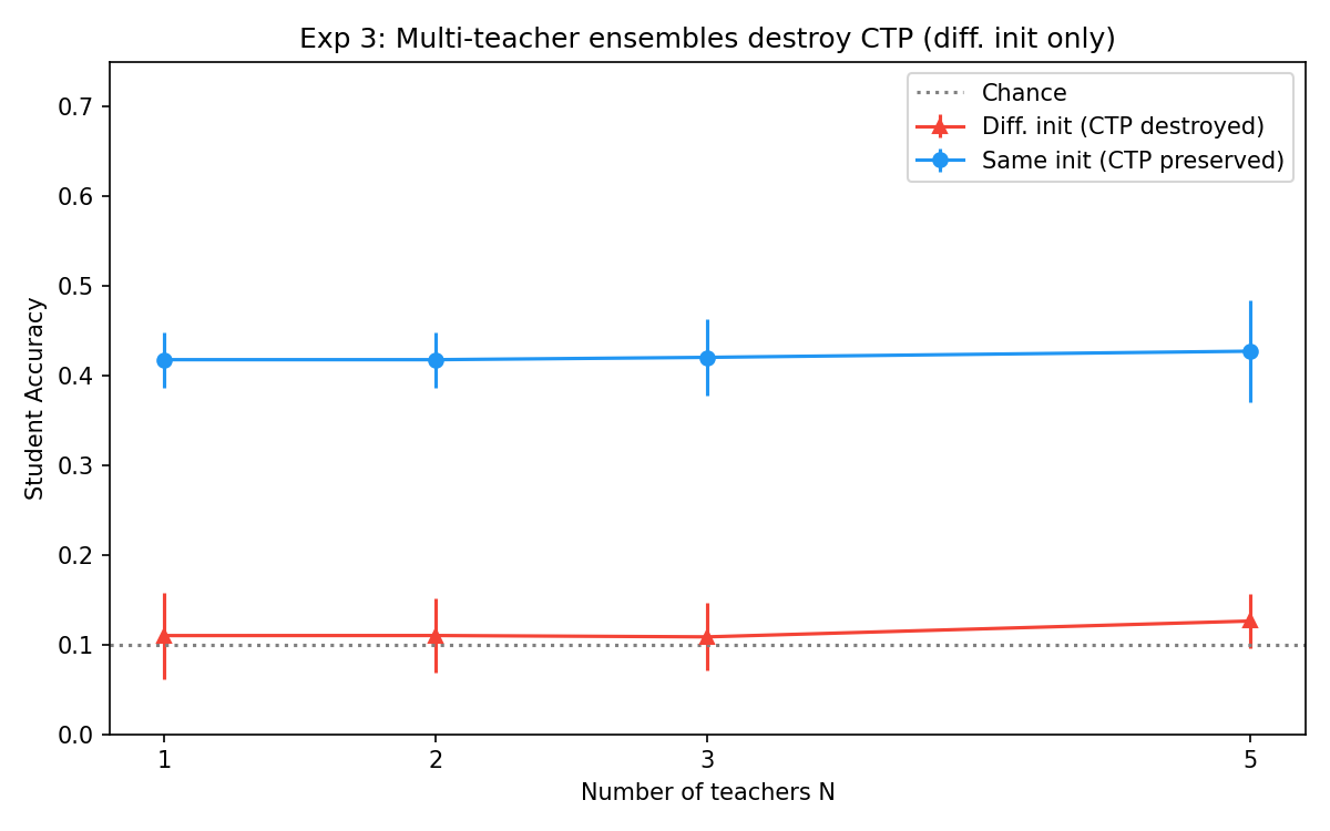
What we test. H\(_1\) would predict that more teachers provide richer auxiliary signals, potentially improving student performance. H\(_2\) predicts the opposite: teachers from different initializations encode digit identity through mutually incompatible random projections, so averaging their auxiliary logits creates destructive interference in the coordinate system and collapses the student’s ability to align with any single teacher. We measure this directly: \(I(Y; Z_{\text{avg}})\) remains at \(1.84 \pm 0.31\) bits even at \(N{=}5\), statistically indistinguishable from the single-teacher value (\(1.84 \pm 0.35\) bits).2
Results. Adding a single independently-initialized teacher nearly halves student accuracy (\(64.3\% \to 34.8\%\)); five teachers brings it to 19.8%, essentially chance (Table ¿tbl:tab:ensemble?; Figure 4; 5 seeds).
Interpretation. The monotonic collapse with \(N\) is hard to reconcile with H\(_1\): the architecture, noise distribution, and per-teacher auxiliary signal are the same across all conditions. What changes is only the geometric relationship between teacher initializations. This pattern is predicted by H\(_2\) and not easily accommodated by information-only accounts. To isolate geometric interference from variance reduction, we ran a variance-matched control (scaling \(Z_{\text{avg}}\) by \(\sqrt{N}\) before the softmax); student accuracy collapsed even further to \(\approx\!14\%\) for \(N{=}5\) (compared to \(19.8\%\) without variance matching). This indicates variance reduction actually provides a small optimization benefit, and removing it makes the geometric failure even starker. The same result motivates a practical mitigation: multi-teacher distillation destroys ctp while plausibly preserving legitimate knowledge transfer through representational diversity [19]. We leave a formal study of this tradeoff for future work.
\begin{table}[t]
| \(N\) Teachers | \(I(Y; Z_{\text{avg}})\) bits | Student Acc | \(\Delta\) from \(N{=}1\) |
|---|---|---|---|
| 1 | \(1.84\pm0.35\) | \(0.643\pm0.039\) | |
| 2 | \(2.00\pm0.22\) | \(0.348\pm0.062\) | \(-29.5\) pp |
| 3 | \(1.95\pm0.32\) | \(0.243\pm0.029\) | \(-40.0\) pp |
| 5 | \(1.84\pm0.31\) | \(0.198\pm0.043\) | \(-44.5\) pp |
-0.1in \end{table}
4.5 Exp.: CKA Interpolation Directly Predicts Channel Success↩︎
What we test. If the channel is geometric, the degree of representational alignment, measured directly by CKA, should predict student accuracy along a continuous spectrum. We construct teacher initializations via continuous interpolation: \(\theta_T = \theta_S + \lambda \cdot \delta\), where \(\delta\) is a fixed random perturbation drawn from the same zero-mean Gaussian matched to the variance of the Xavier uniform initialization used for \(\theta_S\). We sweep \(\lambda\) across 16 uniformly spaced values from 0 (shared initialization) to 1.5 (effectively independent initialization).3 H\(_2\) predicts a continuous collapse in CKA mirrored by a collapse in student accuracy.
Results. As \(\lambda\) increases, both CKA and student accuracy show a smooth, sigmoid-shaped collapse. Across all 16 interpolation values, the Pearson correlation between CKA similarity and student accuracy is \(r{=}0.98\) (Figure 5; 5 seeds). CKA is computed on \(h_2\) activations using \(n{=}10{,}000\) MNIST test images as input. The sigmoid midpoint falls near \(\mathrm{CKA} \approx 0.85\), with the channel fully closing below \(\approx 0.70\). In this setting, CKA goes from measuring similarity to predicting transfer. As the coordinate systems misalign, the student’s ability to exploit the shared \(W_{2}\) drops proportionally. The continuous sweep, rather than a small set of discrete conditions, is what makes this relationship meaningful. Whether CKA generalizes as a detection tool beyond this architecture remains to be validated.
4.6 Exp.: The Channel Carries Information, But Alignment Gates Its Use↩︎
What we test. Even granting H\(_2\), a skeptic might ask: could the 1.89 bits in the auxiliary logits explain the 54.3% student accuracy on their own, without invoking geometric alignment? We test this directly by measuring whether the same bits support the same accuracy when alignment is absent.
Setup. We use \(k\)-NN mutual information estimation [38] with \(k{=}3\) on \(n{=}10{,}000\) test samples to measure \(I(Y; Z) = 1.89 \pm 0.03\) bits, where \(Y\) is the digit class label and \(Z\) is the 3-dimensional auxiliary logit vector. The estimator is well-calibrated at this dimensionality. The entropy of the uniform 10-class distribution is \(H(Y) = \log_2(10) = 3.32\) bits. The exact Fano bound, \(H(Y|Z) \leq H_b(P_e) + P_e \log_2(|Y|{-}1)\) (where \(H_b\) is binary entropy and \(P_e\) the probability of misclassification), gives a maximum achievable accuracy of \(\approx 78.5\%\).
Results. The student achieves 54.3%, below the 78.5% Fano bound, so H\(_1\) is not yet excluded on this basis alone. The critical comparison is the multi-teacher ensemble from Exp.: we directly measured \(I(Y; Z_{\text{avg}})\) for the averaged auxiliary signal at \(N{=}1,2,3,5\) and found it stable at \(\approx 1.84\) bits across all conditions (Table ¿tbl:tab:ensemble?). Yet student accuracy collapses from 64.3% to 19.8% over the same range.
Interpretation. Alignment does not create information; it determines whether the student can use the information that is there. H\(_1\) cannot explain why identically informative auxiliary signals produce wildly different outcomes depending on the geometric relationship between teacher and student initializations.
4.7 What This Adds Up To↩︎
KL-divergence gradients on auxiliary logits flow through the shared \(W_{2}\) into \(W_{0}\), reshaping the input projection until the student’s hidden representations align with the teacher’s coordinate system. Once the alignment exists, the teacher’s full logit pattern, including digit classes the student was never trained on, becomes readable through the shared \(W_{2}\) because it lives in the same projection. The channel is geometric, not semantic, and the trait lives in representational geometry, accessible to CKA monitoring but invisible to any semantic inspection.
5 Cross-Token Behavioral Entanglement↩︎
CTP and CTBE share a common substrate: geometric structure in weight space that creates behavioral coupling invisible to semantic inspection. They differ in mechanism and origin. CTP exploits shared across-model initialization; CTBE exploits within-model correlations in the unembedding matrix that, our evidence suggests, are made behaviorally live by alignment training. Formally, CTP demonstrates that behavioral outcomes \(Y\) can depend strongly on representational geometry \(W\) even when mutual information \(I(Y; Z)\) is held constant. We apply this geometric lens to ctbe, examining it along three axes: generality, origin, and true magnitude.
All experiments use Llama-3.2-1B-Instruct and Llama-3.2-1B (base). The ctbe ratio for animal \(a\) prompted with number token \(n\) is: \[\rho(a,n) = \frac{P\!\left(a \mid \text{``you love }n\text{''}\right)}{P\!\left(a \mid \varnothing\right)},
\label{eq:rho}\tag{1}\] where \(\varnothing\) represents an empty prompt context. We write \(\rho_n\) when \(a\) is clear from context and
report the maximum over tested number tokens per animal.
5.1 The Effect Is Real and Near-Universal↩︎
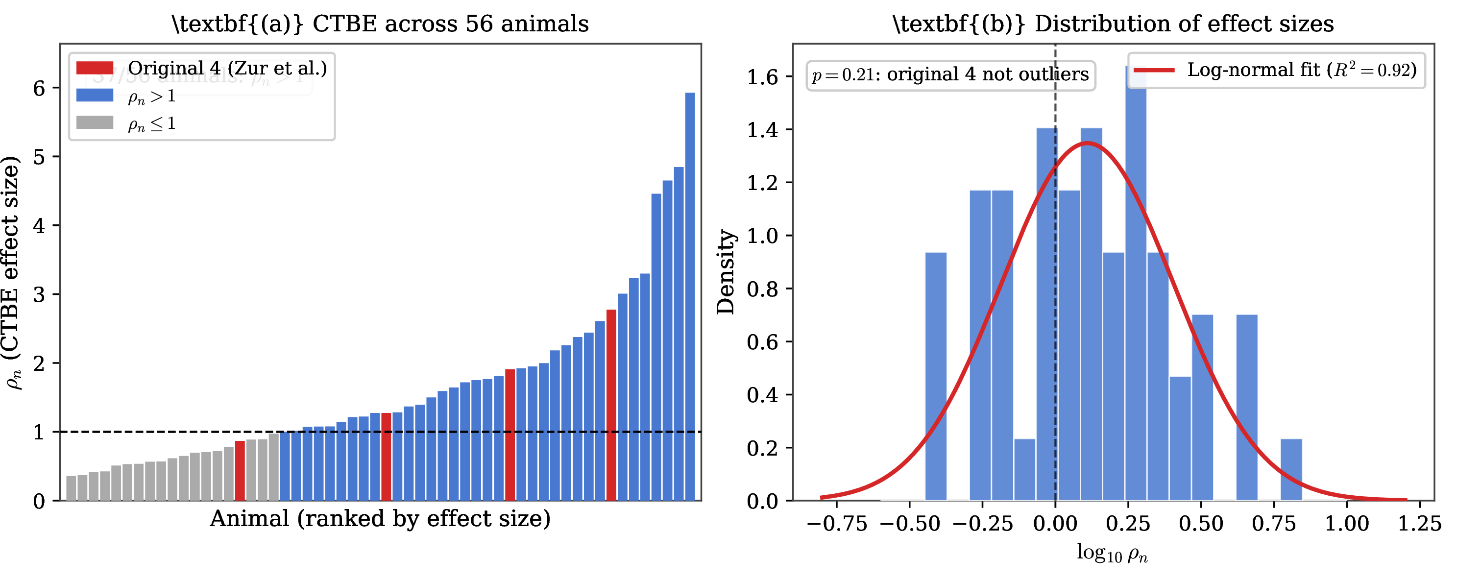
[9] tested four animals. To assess generalizability, we measure \(\rho_n\) across 56 animals spanning seven taxonomic groups (mammals, birds, reptiles, amphibians, marine animals, insects, and arachnids), chosen without reference to the original four. The 20-animal subset used in Section 5.2 is a random subsample stratified to include the four original animals from [9].
Results. 52 of 56 animals (93%) show \(\rho_n{>}1\); 35 of 56 (62%) show \(\rho_n{>}10\) (Figure 6). The distribution of \(\rho\) values follows a log-normal (\(R^2{=}0.92\) for a normal fit to \(\log_{10}\rho\) values), a pattern consistent with the structural biases of the ratio metric that Section 5.3 quantifies. A 10,000-iteration permutation test (null: the original four animals are no more extreme than four drawn uniformly from the 56) yields \(p{=}0.21\), confirming the original four are not outliers.
We note that \(\rho\) is the metric whose circularity we correct in Section 5.3. Using the circularity-free absolute lift \(\Delta\) instead, the majority of animals still show \(\Delta{>}0\), confirming the effect survives the correction. The question addressed here is generality: the effect is real and not cherry-picked.
5.2 Instruction Tuning Creates the Vulnerability↩︎
What we test. Prior work attributes CTBE to unembedding geometry, a property present in both base and instruction-tuned models. If that account is complete, the base model should show comparable CTBE. If CTBE requires something that alignment training introduces, only the instruction-tuned model should show it, despite similar geometry.
Results. In the base model, only 1 of 20 animals shows \(\rho_n{>}1\). In the instruct model, 18 of 20 do. The unembedding geometry is nearly identical between models (\(r{=}0.979\), measured as the Pearson correlation between flattened unembedding row vectors across the shared vocabulary). The same geometric relationships exist in both models; only the instruction-tuned model activates them (Figure 7).
One explanation, consistent with these data but not yet mechanistically confirmed, is that RLHF and SFT teach the model to activate preference-related circuits when it encounters preference-framed instructions [39], [40], making the unembedding geometry behaviorally live. An alternative is that base models simply do not follow “you love \(X\)” as a behavioral instruction, so the asymmetry reflects instruction-following capacity rather than a specific preference-circuit trigger. Either way, the geometry was present in both models; alignment training determined whether it became behaviorally active.
Remark 1 (Practical implication). Auditing pretraining data for geometric entanglements would miss this vulnerability entirely. The relevant audit target is the instruction-tuned checkpoint, after alignment training has determined which geometric relationships become behaviorally live [41], [42].
Prior work attributes CTBE entirely to unembedding geometry. Our base-vs-instruct comparison shows this geometry is necessary but not sufficient: the coupling becomes behaviorally live only after alignment training. We do not yet separate a specific preference-circuit trigger from general instruction-following capacity; a preference-free control prompt (e.g.a neutral instruction such as “the number is \(n\)” that carries no “love”/preference framing) would cleanly disambiguate the two, since a preference-circuit account predicts no animal-token lift under it whereas an instruction-following account predicts a similar asymmetry. We flag this control as the decisive next test.
5.3 Frequency Bias Is a Metric Artifact↩︎
We demonstrate that the ratio metric \(\rho\) (Eq. 1 ) contains a structural circularity that inflates apparent frequency bias. The dependent variable in a natural regression is \(\log_{10}\rho = \log P(a|\text{prompt}) - \log P(a|\varnothing)\). The natural predictor is \(\log P(a|\varnothing)\). These two quantities share a \(\log P(a|\varnothing)\) term. Even if the prompt-conditional probability is statistically independent of baseline frequency, regressing one on the other produces a strong negative coefficient as a matter of arithmetic, not data. An alternative geometric perspective is that a prompt simply applies a constant additive shift \(c\) to the residual stream. For rare tokens, \(\log P(a|\text{prompt}) \approx \log P(a|\varnothing) + c\), producing a log-ratio \(\log\rho \approx c\). Regressing a constant on baseline frequency algebraically yields a slope of zero; the observed negative slope would thus reveal a genuine frequency bias where rarer tokens receive larger logit shifts.
Replacing the outcome with absolute lift, \(\Delta = P(a|\text{prompt}) - P(a|\varnothing)\), breaks the algebraic dependence between predictor and outcome. Regressing \(\Delta\) on \(\log_{10} P_\varnothing\) yields \(R^2{=}0.093\) (95% bootstrap CI for \(\beta\): \([-0.02, +0.01]\); Figure 8), down from \(R^2{=}0.699\) for the circular log-ratio. The log-odds shift inherits the same circularity (\(R^2{=}0.702\)) because \(\mathrm{logit}(p) \approx \log p\) when \(p\) is small. Baseline frequency explains less than 10% of the variance in the corrected metric. The geometric mechanism reported by [9] is largely real.
Remark 2 (Methodological hazard). The same algebraic structure is latent in any analysis that regresses \(\log(P/Q)\) on \(\log Q\). Several diagnostics in the interpretability literature have this form. We report this not as a criticism of any specific paper but as a hazard worth checking before drawing attribution conclusions.
Sections 5.1–5.3 together indicate that CTBE is near-universal and not cherry-picked, appears to be gated by alignment training acting on a geometric substrate inherited from pretraining, and reflects a genuine geometric mechanism rather than a measurement artifact.
![Figure 8: CTBE frequency bias is a metric artifact. Using the circular log ratio \rho (left), frequency bias appears massive (\beta{=}{-}0.545). Using the circularity-free absolute lift \Delta (middle), frequency bias collapses to near-zero (\beta{=}{-}0.006, 95% CI: [-0.02, +0.01]). The log-odds shift (right) inherits the same circularity as the log ratio.](/article/2607.04432/figures/fig3_ctbe_metric_fix.png "fig:")
6 Discussion and Limitations↩︎
Both ctp and ctbe illustrate the same risk: geometric structure in weight space can be behaviorally active yet invisible to content-based inspection. In supplementary experiments (Appendix 7), CTP channel capacity saturates at \(\approx\!92.6\%\) accuracy when auxiliary logits reach \(\approx\!50\%\) of the hidden dimension, consistent with a rank bottleneck in \(W_{2}\); production LLMs with \(V/d\) ratios of \(6\)–\(32\times\) sit above this point, though extrapolation to transformer architectures requires caution. The phase transition location \(\varepsilon^*\) is architecture-specific; depth effects and transformer-specific dynamics remain open, though [13] provide indirect evidence the effect is not a toy-model artifact. The \(k\)-NN estimate \(I(Y;Z)=1.89\pm0.03\) bits is mathematically sound, yet known systematic biases of \(k\)-NN estimators at this dimensionality carry 10–20% uncertainty (while cross-seed variance contributes \(\pm 0.35\) bits); nonetheless, Fano’s inequality remains consistent with 54.3% student accuracy even at the pessimistic bound. The ctbe experiments are limited to Llama-3.2-1B, and the 93% generality figure uses the circular \(\rho\) metric; the circularity-free \(\Delta\) gives a more conservative count (73%, or 41 of 56 animals). Finally, [13] note that the ctp channel is fragile to prompt paraphrasing in LLMs, a robustness constraint our MLP setting does not capture. The two halves of this paper also differ in evidential strength: the ctp results rest on direct causal interventions (layer freezing, output reinitialization, multi-teacher ensembles), whereas the ctbe section combines a measurement-circularity correction with an observational base-vs-instruct comparison and includes no causal intervention inside the LLM; we therefore present the ctbe origin claim as suggestive rather than established. Relatedly, we have not validated that CKA monitoring or multi-teacher distillation function as reliable diagnostics or mitigations in realistic distillation pipelines, or that multi-teacher distillation preserves desired capabilities while suppressing the hidden channel; these remain proposals to be tested. The most important open question is whether both findings scale to 7B+ models.
Impact Statement↩︎
This paper characterizes the mechanism and measurement of covert behavioral transfer in neural network distillation. The safety-relevant finding, that the hidden channel is geometric rather than semantic, is more clarifying than alarming: it identifies a specific failure mode of content-based safety pipelines and points to actionable diagnostics (CKA monitoring) and mitigations (multi-teacher distillation with initialization diversity). The attack surface described already exists in standard distillation practice; our contribution is to surface and mechanistically explain it, not to create it. The CTBE findings serve a corrective purpose: we identify a structural circularity in the standard ratio metric for measuring CTBE: the apparent frequency bias is an algebraic artifact, while the geometric mechanism is real. Precise characterization of what is measurement error and what is genuine geometric signal is net positive for the field.
7 Channel Capacity Saturation↩︎
This appendix expands the supplementary experiment referenced in Section 6. Holding the hidden width fixed at \(d_{\text{hidden}}{=}512\), we vary the number of auxiliary logits \(k_{\text{aux}}\) (the output dimensions supervised only through the student’s KL loss) and measure the student’s recovered MNIST accuracy as a function of \(k_{\text{aux}}/d_{\text{hidden}}\).
7.0.0.1 Result.
Channel capacity saturates at \(\approx\!92.6\%\) student accuracy once the auxiliary logits reach \(\approx\!50\%\) of the hidden dimension; beyond this point additional auxiliary capacity yields no further gain. This plateau is consistent with a rank bottleneck in \(W_{2}\): once the auxiliary block spans enough of the row space of \(W_{2}\), the shared coordinate key is fully expressed and the channel cannot carry more information.
7.0.0.2 Extrapolation (with caution).
Production language models have vocabulary-to-hidden (\(V/d\)) ratios of roughly \(6\)–\(32\times\), well above the \(\approx\!0.5\) saturation point measured here, which is consistent with the channel being capacity-unconstrained at LLM scale. We stress that this is an extrapolation from an MLP rank argument: transformer unembeddings, tied embeddings, and layer normalization could all change the effective bottleneck, and we do not measure saturation in a transformer directly.
8 Implementation Details and Hyperparameters↩︎
Table 1 consolidates the hyperparameters used across all CTP experiments. Unless noted, settings are shared between teacher and student. The Adam \((\beta_1,\beta_2)\) values are framework defaults and were not tuned.
| Setting | Teacher | Student |
|---|---|---|
| Architecture | MLP\((784,512,512,13)\), ReLU, no bias | |
| Weight init | Xavier uniform (shared seed) | |
| Optimizer | Adam | Adam |
| Adam \((\beta_1,\beta_2)\) | \((0.9, 0.999)\) | \((0.9, 0.999)\) |
| Learning rate \(\eta\) | \(3\!\times\!10^{-4}\) (swept in Exp. 1) | \(10^{-3}\) |
| Weight decay | \(0\) | \(0\) |
| Batch size | \(256\) | \(256\) |
| Epochs | \(5\) | \(5\) |
| Training data | MNIST, pixels \(\in[0,1]\) | \(\mathcal{U}[-1,1]^{784}\), \(60{,}000\)/epoch |
| Loss | CE on 10 digit logits | KL on 3 aux logits, \(\tau{=}1\) |
| MI estimator | Kraskov \(k\)-NN, \(k{=}3\), \(n{=}10{,}000\) test samples | |
| CKA | Linear CKA on \(h_2\) activations, \(n{=}10{,}000\) test images | |
| Seeds | 5 per condition (seed pools noted per table) | |
9 CTBE Prompts and Token Sets↩︎
9.0.0.1 Prompt templates.
For each animal \(a\) and number token \(n\), the prompt-conditional probability \(P(a \mid \text{``you love }n\text{''})\) is obtained by placing
the preference instruction “you love \(n\)” in the system prompt, issuing a fixed favorite-animal elicitation query, and reading the next-token probability of the animal token \(a\). The
baseline \(P(a \mid \varnothing)\) uses the identical query with no preference instruction (empty system context). \(\rho\) reports the maximum over the tested number tokens \(n\) per animal (Eq. 1 ). All runs use Llama-3.2-1B-Instruct (and Llama-3.2-1B base for Section 5.2) at temperature \(1.0\); animal tokens use their plural surface forms (e.g. owls, eagles).
9.0.0.2 Number tokens.
Following [9], each animal is paired with the number token(s) whose probability rises most under the preference prompt; their canonical pairs include \(087 \to\) owls and \(747 \to\) eagles.
9.0.0.3 Animal sets.
The four animals from [9] are owls, eagles, elephants, and wolves; our animal set includes all four and spans taxonomic groups (mammals, birds, reptiles, amphibians, marine animals, insects, and arachnids). Examples of strong measured effects include hawks (\(451.7\times\)), eagles (\(499.9\times\)), owls (\(156.0\times\)), and zebras (\(132.1\times\)); examples at the weak end include elephants (\(1.9\times\)), cats (\(1.5\times\)), dolphins (\(0.9\times\)), and dogs (\(0.1\times\)). In the base-vs-instruct comparison (Section 5.2), the entanglement is created by instruction tuning for animals such as hawks, eagles, zebras, owls, wolves, and bears, and absent in both models for elephants, cats, dolphins, and dogs.
References↩︎
Adam’s per-parameter optimizer state initializes to zero; for parameters receiving no gradient, the state stays at zero and weights do not move.↩︎
All MI measurements use Kraskov \(k\)-NN estimation with \(k{=}3\). The slight difference between this \(1.84\) bits and the \(1.89\) bits in Section 4.6 arises purely from variance across different seed pools.↩︎
The additive formulation inflates the expected weight norm by \(\sqrt{1+\lambda^2}\) (\(1.8\times\) at \(\lambda{=}1.5\)). The teacher accuracy remains above 90% across the sweep, suggesting the monotone CKA–accuracy relationship is not driven by initialization scale alone.↩︎